GLOBAL MODELS OF SPATIAL VARIATION IN ATMOSPHERIC ∆¹⁴C

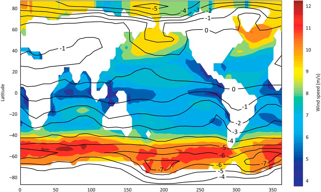
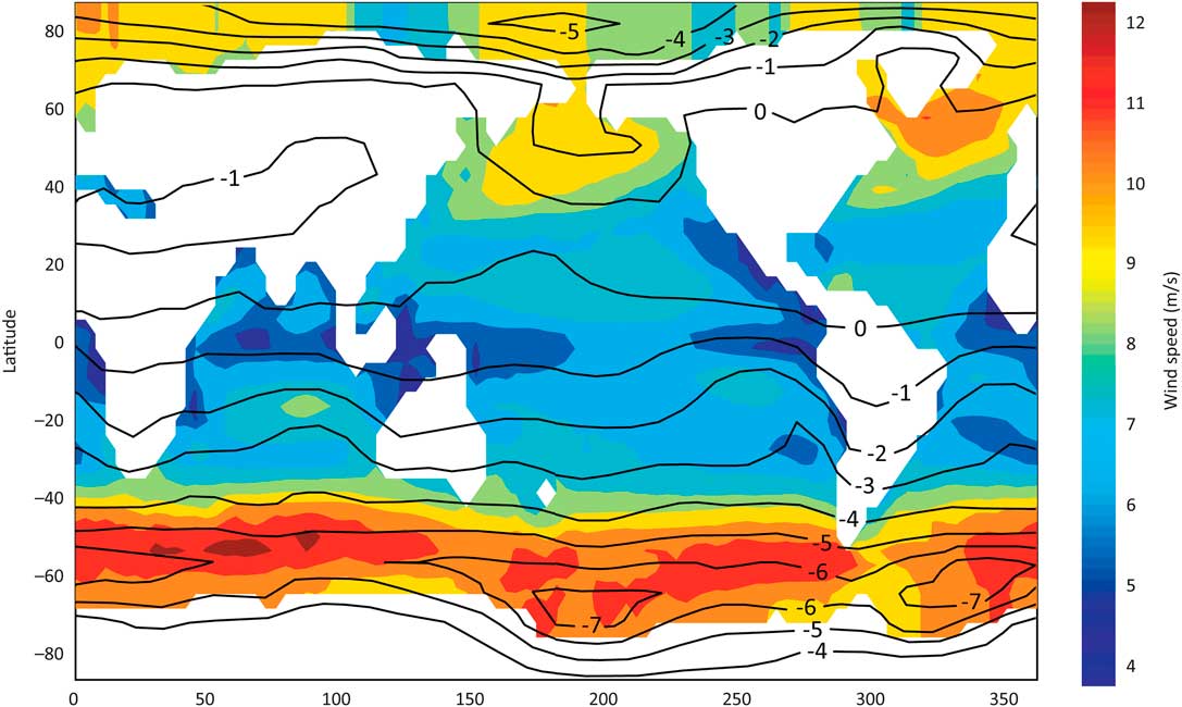
The Southern Hemisphere has lower ∆¹⁴C values than the Northern Hemisphere, which results in older ¹⁴C dates for tree rings of the same calendar year (Lerman et al. Reference Lerman, Mook and Vogel1970; McCormac et al. 1998, 2002, Reference McCormac, Hogg, Blackwell, Buck, Higham and Reimer2004; Stuiver and Braziunas Reference Stuiver and Braziunas1998). This difference has been attributed to the fact that the Southern Hemisphere has more of the world’s ocean surface area: 61%, in contrast with 39% in the Northern Hemisphere (Braziunas et al. Reference Braziunas, Fung and Stuiver1995; Stuiver and Braziunas Reference Stuiver and Braziunas1998:331). Air–sea exchange of CO₂ injects relatively old carbon from the surface ocean into the atmosphere (see overviews in Dutta Reference Dutta2016; Turnbull et al. Reference Turnbull, Graven and Krakauer2016), an effect that is strongest in the Southern Ocean surrounding Antarctica (Anderson et al. Reference Anderson, Ali, Bradtmiller, Nielsen, Fleisher, Anderson and Burckle2009; Franke et al. Reference Franke, Paul and Schulz2008; Rodgers et al. Reference Rodgers, Mikaloff-Fletcher, Bianchi, Beaulieu, Galbraith, Gnanadesikan, Hogg, Iudicone, Lintner, Naegler, Reimer, Sarmiento and Slater2011). Here, strong winds induce upwelling of “old” deep water to the surface and into the atmosphere, to be subsequently mixed northward throughout the Southern Hemisphere (Krakauer et al. Reference Krakauer, Randerson, Primeau, Gruber and Menemenlis2006; Rodgers et al. Reference Rodgers, Mikaloff-Fletcher, Bianchi, Beaulieu, Galbraith, Gnanadesikan, Hogg, Iudicone, Lintner, Naegler, Reimer, Sarmiento and Slater2011). On a global scale, predominantly zonal winds in both hemispheres result in east–west zonal bands of different atmospheric ¹⁴C concentrations. Winds are generally stronger near the poles and weaker in the tropics, resulting in a modeled north-to-south gradient of roughly 1‰ less ¹⁴C (8 ¹⁴C yr older) per 10° of latitude (Figure 1), as compared to levels in the Northern Hemisphere (Levin et al. Reference Levin, Kromer, Wagenbach and Münnich1987; Braziunas et al. Reference Braziunas, Fung and Stuiver1995; Krakauer et al. Reference Krakauer, Randerson, Primeau, Gruber and Menemenlis2006).

Figure 1

Global wind speeds (from Krakauer et al. Reference Krakauer, Randerson, Primeau, Gruber and Menemenlis2006: Figure 1) and the latitudinal ¹⁴C gradient (from Braziunas et al. Reference Braziunas, Fung and Stuiver1995: Figure 9a). Contours show the difference (‰) from atmospheric carbon near Seattle. Note the strong correlation between winds and carbon depletion near Antarctica, which affects the entire hemisphere.

Global models are a useful first approximation to potential regional variation in ∆¹⁴C but are based primarily on marine data. Past terrestrial variations of atmospheric ∆¹⁴C values are best determined with tree-ring ¹⁴C dates. Models and tree-ring data broadly agree on an interhemispheric ∆¹⁴C difference of 3–5‰, based on comparisons between tree rings from mid-latitudes in the Northern (53–54°N) and Southern (39°S) Hemispheres (McCormac et al. Reference McCormac, Hogg, Higham, Lynch-Stieglitz, Broecker, Baillie, Palmer, Xiong, Pilcher and Brown1998:1323; Krakauer et al. Reference Krakauer, Randerson, Primeau, Gruber and Menemenlis2006:407). This is consistent with modern air differences of 3–4‰ between Northern and Southern Hemisphere data recorded in the western Pacific Ocean (Kitagawa et al. Reference Kitagawa, Mukai, Nojiri, Shibata, Kobayashi and Nojiri2004). Other than this clear interhemispheric difference, proposed regional variations in atmospheric ¹⁴C have not been confirmed. Some tree-ring datasets have unexplained offsets that are not included in current calibration curves and do not always follow the expectations of global models (see Stuiver and Braziunas 1993, Reference Stuiver and Braziunas1998; Reimer et al. Reference Reimer, Baillie, Bard, Bayliss, Beck, Bertrand, Blackwell, Buck, Burr, Cutler, Damon, Edwards, Fairbanks, Friedrich, Guilderson, Hogg, Hughen, Kromer, McCormac, Manning, Bronk Ramsey, Reimer, Remmele, Southon, Stuiver, Talamo, Taylor, van der Plicht and Weyhenmeyer2004). Future research is required to determine whether differences are statistically significant and, if so, what may cause them, for example, regional ¹⁴C variation, diachronic ¹⁴C variation, or inter-laboratory differences (McCormac et al. Reference McCormac, Reimer, Hogg, Higham, Baillie, Palmer and Stuiver2002; Hogg et al. 2011, 2013a, Reference Hogg, Turney, Palmer, Cook and Buckley2013b).

Braziunas et al.’s (1995: Figure 9a) global model of ∆¹⁴C concentrations suggests spatial differences in ¹⁴C concentrations in South America. It estimates that concentrations at ~0–30° S in South America are 1–2‰ lower than in the Northern Hemisphere, roughly half of the difference documented in higher latitude tree-rings from the Southern Hemisphere (Figure 1). Following this, a recent model of Holocene ¹⁴C used an arithmetic mean of IntCal and SHCal for tropical regions between 20°N and 20°S (Roth and Joos Reference Roth and Joos2013:1884). This sensible approach was used because the two curves are derived from mid-latitude tree rings, so low-latitude tree rings should have intermediate dates somewhere between those of the two curves. Low-latitude dates could potentially be modeled to have greater error ranges, because carbon concentrations in the tropics and neo-tropics are not well defined (McCormac et al. Reference McCormac, Hogg, Blackwell, Buck, Higham and Reimer2004:1088).

The picture is complicated by diachronic shifts in inter-hemispheric carbon differences, which have varied over time by 1–10‰ (McCormac et al. Reference McCormac, Hogg, Blackwell, Buck, Higham and Reimer2004:1088). For the period 200 BC–AD 1850, SHCal13 calibrated ages range from 2 ¹⁴C yr younger to 83 ¹⁴C yr older than IntCal ages, with a periodicity of ~130 yr (McCormac et al. Reference McCormac, Reimer, Hogg, Higham, Baillie, Palmer and Stuiver2002:641; Hogg et al. 2009, 2011, Reference Hogg, Hua, Blackwell, Niu, Buck, Guilderson, Heaton, Palmer, Reimer and Reimer2013a:1889). Dendrochronological evidence suggests that the inter-hemispheric ¹⁴C difference was reduced to nearly zero at the end of the Little Ice Age (Turney et al. Reference Turney, Palmer, Hogg, Fogwill, Jones, Ramsey, Fenwick, Grierson, Wilmshurst, O’Donnell, Thomas and Lipson2016). Temporal variation in the inter-hemispheric difference seems to be correlated with modes of variation in atmospheric circulation, such as the El Niño–Southern Oscillation (ENSO) (Turney and Palmer Reference Turney and Palmer2007:175).

The inter-hemispheric difference also varies seasonally, specifically near the equator during monsoon seasons, when air masses can move north or south across the tropical equator (Rozanski et al. Reference Rozanski, Levin, Stock, Falcon and Rubio1995; Hua et al. Reference Hua, Barbetti and Zoppi2004a; Kitagawa et al. Reference Kitagawa, Mukai, Nojiri, Shibata, Kobayashi and Nojiri2004; Hua and Barbetti Reference Hua and Barbetti2007). This is not accounted for by current carbon models or calibration curves but is a factor at low latitudes. It is best quantified with ¹⁴C measurements of tree-rings during the post-bomb era, because the large quantities of carbon released in nuclear testing amplify regional differences (Hua et al. Reference Hua, Barbetti and Rakowski2013). Based on cross-dated Pinus kesiya tree rings in Thailand, Hua and Barbetti (Reference Hua and Barbetti2007:8) estimated a 52±13% contribution of Southern Hemisphere air masses during the Southwest Asian monsoon in pre-bomb years (this estimate could be used in OxCal’s mixed curve calibration; see below). In Japan, a large set of prehistoric tree-ring dates showed significant differences from IntCal, which the authors attributed to monsoon input of air from the Southern Hemisphere (Suzuki et al. Reference Suzuki, Sakurai, Takahashi, Sato, Gunji, Tokanai, Matsuzaki and Tsuchiya2010:1606). For South America, bomb-era ¹⁴C dates from Amazonian trees suggest a close match to SHCal (Jenkins Reference Jenkins2009; Andreu-Hayles et al. Reference Andreu-Hayles, Santos, Herrera-Ramírez, Martin-Fernández, Ruiz-Carrascal, Boza-Espinoza, Fuentes and Jørgensen2015; Santos et al. Reference Santos, Linares, Lisi and Tomazello Filho2015), but there are not yet sufficient data to assess or quantify potential CO₂ contributions from the Northern Hemisphere. Future research may user older tree rings from different altitudes and latitudes to refine spatial and temporal ∆¹⁴C variation in South America due to factors such as altitude, latitude, period, and region (see Jenkins et al. Reference Jenkins, Baker and Negrón-Juárez2013; Morales et al. Reference Morales, Nielsen and Villalba2013).

DEFINING HEMISPHERIC MIXING AND AIR MASS SOURCES IN TROPICAL SOUTH AMERICA

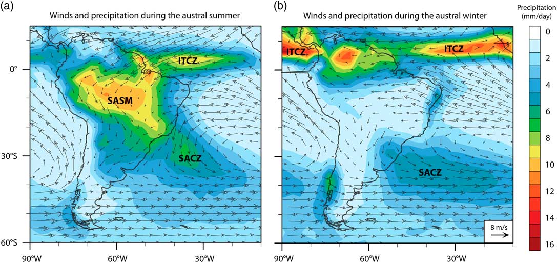
Despite its name, which implies a global reach, IntCal is based on samples from temperate latitudes (47–54°N) of the Northern Hemisphere. Similarly, SHCal is derived from tree-ring measurements from mostly temperate latitudes in New Zealand (40°S), Chile (55°S), South Africa (21–33°S), and Tasmania (42°S) (see citations in Hogg et al. Reference Hogg, Hua, Blackwell, Niu, Buck, Guilderson, Heaton, Palmer, Reimer and Reimer2013a:1890). Given the latitudinal gradient of ¹⁴C, these curves are most appropriate at the same latitudes of the trees used for calibration, but may not be appropriate for the under-sampled tropics. Assuming well-mixed atmospheres within each hemisphere, McCormac et al. (Reference McCormac, Hogg, Blackwell, Buck, Higham and Reimer2004:1088) and Hogg et al. (Reference Hogg, Hua, Blackwell, Niu, Buck, Guilderson, Heaton, Palmer, Reimer and Reimer2013a:1900) have suggested that the thermal equator or Intertropical Convergence Zone (ITCZ) should be used to delimit the spatial boundary between the two curves. Their data show a well-mixed Southern Hemisphere atmosphere, at least at the latitudes of their sampled sites. However, using the ITCZ as an operational boundary is problematic, because it is a marine phenomenon that is not clearly defined over the continents. Moreover, it moves seasonally and over longer paleoclimatic time scales (Haug et al. Reference Haug, Hughen, Sigman, Peterson and Röhl2001; Schneider et al. 2014). The lack of clarity regarding the zonal boundaries of atmospheric mixing between the two hemispheres warrants a more careful consideration of South American climate. Specifically, we address spatio-temporal patterns and amounts of inter-hemispheric atmospheric transport. The ITCZ is a zone of atmospheric convergence over the oceans (Figure 2), which migrates in response to variation in latitudinal temperature gradients (Chiang and Blitz Reference Chiang and Bitz2005). The ITCZ has a direct influence on the climatology of coastal regions of northeastern South America, including the northern Nordeste of Brazil (Hastenrath and Heller Reference Hastenrath and Heller1977) and the north coast of Venezuela (Poveda et al. Reference Poveda, Waylen and Pulwarty2006). ITCZ variability also may affect the climate inland of these regions by controlling the strength and trajectory of the advection of air and moisture onto the continent (Curtis and Hastenrath Reference Curtis and Hastenrath1999).

Figure 2

Major climate systems and long-term (1979–2010) means of precipitation and winds at 925 hPa in South America, showing average values during (a) the austral summer (December–February) and (b) the austral winter (July–August), based on data from the Climate Prediction Center merged analysis of precipitation (Xie and Arkin Reference Xie and Arkin1997).

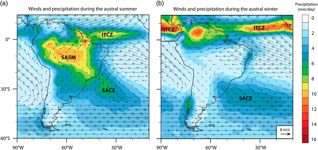
The ITCZ does not extend across the continent (Cook Reference Cook2009; Baker and Fritz Reference Baker and Fritz2015), despite being commonly misrepresented this way in many paleoenvironmental and archaeological publications. Rather, low-level convergence over the southern tropical continent during the austral summer is a separate feature of the South American summer monsoon (SASM). The SASM is a near continental-scale circulation system that advects air and moisture from the tropical Atlantic Ocean across the Amazon Basin, southeastward along the eastern flank of the Andes in a low-level jet and exits the continent in the region of the South Atlantic Convergence Zone (SACZ) (e.g. Zhou and Lau 1998; Garreaud et al. Reference Garreaud, Vuille, Compagnucci and Marengo2009; Jones and Carvalho Reference Jones and Carvalho2013; Novello 2017). The intensity of the SASM is strongest in the austral summer (December–February). Over much of tropical and subtropical South America south of the equator, the majority of annual precipitation occurs during this monsoon season (Garreaud Reference Garreaud2009). Inter-annual variation in the SASM is associated with sea-surface temperature gradients in the tropical Atlantic and increased flow associated with an anomalously cold North Atlantic (Nobre and Shukla 1996; Chang et al. 1997). On paleoclimatic time scales, temporal changes in SASM intensity are forced by variation in insolation, greenhouse gas concentrations, glacial boundary conditions, and remote ocean–atmosphere interactions (Vuille et al. Reference Vuille, Burns, Taylor, Cruz, Bird, Abbott, Kanner, Cheng and Novello2012; Baker and Fritz Reference Baker and Fritz2015).

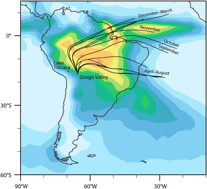
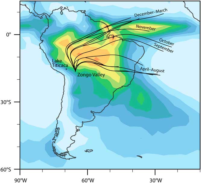
Low-level atmospheric transport into the Amazon Basin is predominantly derived from the equatorial and tropical southern Atlantic during the austral winter (Curtis and Hastenrath Reference Curtis and Hastenrath1999) (Figure 2a). During the austral summer, backtrajectory LaGrangian analyses of low-level flow across the continent (Figure 3) indicate that air masses from the northern tropical Atlantic are the dominant moisture source for the northern Amazon, the eastern Andes, and the adjacent Altiplano (Vimeux et al. Reference Vimeux, Gallaire, Bony, Hoffmann and Chiang2005; Insel et al. Reference Insel, Poulsen, Sturm and Ehlers2013; Sturm et al. Reference Sturm, Hoffmann and Langmann2007). This flow extends to regions as far south as 35°S, although most moisture and strong winds dissipate around 20–25°S (Cook Reference Cook2009; Garreaud Reference Garreaud2009). As this flow moves across the continent, air masses originating in the tropical Atlantic are modified by land-surface processes, as documented in the distillation of water isotopes such as δD (Vimeux et al. Reference Vimeux, Gallaire, Bony, Hoffmann and Chiang2005) and δ¹⁸O (Insel et al. Reference Insel, Poulsen, Sturm and Ehlers2013). During winter months (April–August), air masses originating in the South Atlantic (friajes) reach as far north as ~10°N, but they transport less moisture than summer flows.

Figure 3

Backtrajectories of moisture sources for the Zongo Glacier in Bolivia near Lake Titicaca based on δD (from Vimeux et al. Reference Vimeux, Gallaire, Bony, Hoffmann and Chiang2005:Figure 5). Each line represents the dominant moisture trajectory per month. The base map shows summer precipitation as in Figure 2a. See Vimeux et al. (Reference Vimeux, Gallaire, Bony, Hoffmann and Chiang2005:Figure 6) for monthly images of precipitation and backtrajectories.

Because CO₂, unlike water vapor, is well mixed through the vertical column and has a different source function than water vapor, its seasonal variation of source and trajectory are different from (and less well-known) than those of the predominantly low-level water vapor. In the absence of good regional information on spatial patterns of ¹⁴C variation, we use SASM circulation as an admittedly imperfect foundation for assessing sources of ¹⁴C to continental regions of tropical South America.

The circulation of the SASM takes places during the rainy austral summer (Figure 2b). Even for equatorial locales of the Amazon basin, there is a pronounced increase in precipitation during the SASM season, which is the growing season for deciduous and annual plants. However, it has recently been shown (Wu et al. 2016) that ecosystem primary productivity is quite variable across the basin: forests located in wetter, less seasonal, equatorial regions tend to “green up” during the dry season, while in drier, more seasonal, sub-equatorial regions ecosystem-scale primary productivity varies with seasonal precipitation variation. On the dry and highly seasonal Altiplano, carbon uptake by plants is strongly correlated with seasonal precipitation amount. On the eastern slopes of the Andes, backtrajectories suggest that there is a clear influence of Northern Hemisphere moisture for five months of the year, November–March (Figure 3). Hence, carbon uptake during these months very likely includes carbon that originates from the Northern Hemisphere, both today and during analogous intervals of the past. The influence of SASM suggests that the carbon concentrations of these regions are likely somewhere between the concentrations represented by IntCal and SHCal. This agrees with global models’ expectations for ¹⁴C concentrations at these latitudes of South America (Figure 1). The boundaries of the SASM include the eastern Andes to the the west and go as far south as 35°S. Because winds and SASM precipitation dissipate around 20–25°S, we use this as the approximate southern edge of the SASM-influenced area, though the boundaries remain poorly defined. It is not currently possible to define this area better, which could be a focus of future research.

Various paleoclimatic data have been used to infer changes in the mean position of the ITCZ in oceanic regions adjacent to tropical South America (Haug et al. Reference Haug, Hughen, Sigman, Peterson and Röhl2001; Sachs et al. Reference Sachs, Sachse, Smittenberg, Zhang, Battisti and Golubic2009; Nace et al. Reference Nace, Baker, Dwyer, Silva, Rigsby, Burns, Giosan, Otto-Bliesner, Liu and Zhu2014), as well as variation in the intensity of the SASM at decadal to orbital time scales (Baker and Fritz Reference Baker and Fritz2015). Yet these inferences of past changes in atmospheric circulation are spatially imprecise, so it also is unclear where paleoclimate variation affected air mass transport and spatial variation in ¹⁴C over the continent. These limitations constrain our ability to infer the spatio-temporal variations of past circulations and place more exact limits of the appropriate use of IntCal or SHCal in the past.

In terms of defining areas for each calibration curve, we can draw on the following salient points from the modern climate of South America.

1. 1. The ITCZ mixes air masses over the oceans and its influence on inland areas is indirect. Hence its position does not provide a clear spatial limit of where SHCal is valid in tropical South America.

2. 2. Atmospheric circulation over tropical and subtropical South America is strongly influenced by the SASM, a circulation system that brings Northern Hemisphere air—and likely carbon—into large parts of the Amazon and eastern Andes during the austral summer, which is the primary plant growing season in many areas.

3. 3. SASM circulation provides a good initial approximation of where air masses and ¹⁴C from the two hemispheres may be mixing, although it is unclear how carbon concentrations change as low-level air flows inland.

4. 4. Various aspects of atmospheric circulation (ITCZ position, SASM strength, westerlies) have changed on decadal to orbital scales throughout the Holocene. These changes are imprecisely known, hence the position, spatial footprint, and temporal variation of circulation are necessarily imprecisely defined.

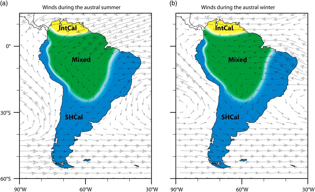
Based on these large-scale modern patterns, we propose the following regions for three different calibration curves (Figure 4). These areas are defined at a continental scale, based primarily on modern wind patterns but also precipitation location and intensity (Figure 2), as well as global ¹⁴C gradients (Figure 1).

1. 1. Northern South America is little influenced by Southern Hemisphere air in any season. Most likely, carbon concentrations are close to those used to define IntCal.

2. 2. In the areas where SASM circulates in the Amazon and eastern Andes, plants likely have a significant uptake of Northern Hemisphere air. The degree of mixing with Southern Hemisphere air remains unknown, but probably dissipates towards the eastern and southern boundaries. Hence a mixed calibration curve that allows for variation between both IntCal and SHCal may be appropriate.

3. 3. South and east of the SASM-influenced Amazon and Andes, there is little to no mixing of Northern Hemisphere air. Along the Pacific coast of tropical South America, south of the equator, southeasterly trade winds tend to dominate circulation year-round, so even at low latitudes, there is likely little input of Northern Hemisphere air. Hence carbon concentrations in this region should track SHCal.

Figure 4

Suggested calibration curves for different parts of South America and winds during the austral (a) summer and (b) winter. The boundaries between the areas are not clear, but are generally estimated as the extension of the area affected by the SASM, which receives strong inputs from part of the Atlantic Ocean in the Northern Hemisphere (Figures 2–3). The southern and western boundaries of the area for the mixed curve are based primarily on SASM wind and precipitation during the austral summer (Figure 2a); the northern boundary is based primarily on patterns during the austral winter (Figure 2b).

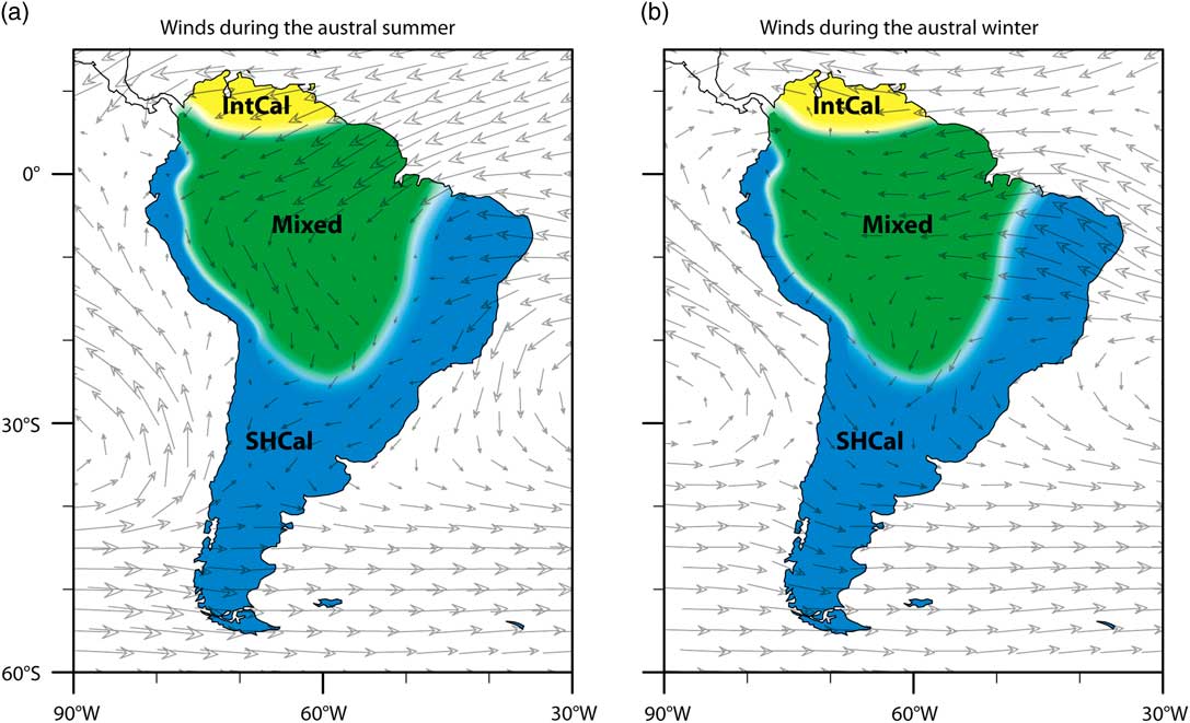
The limits between these three regions remain unclear and cannot be reliably defined on small spatial scales, not to mention diachronic shifts. For researchers working in areas of the SAMS-influenced zone, we recommend using a mixed calibration curve, which is appropriate for areas with known or potential SASM influence because it allows for any degree of mixing, including none, of the ¹⁴C of the two hemispheres. This approach may also be useful for researchers working at tropical latitudes on other continents.

APPLYING A MIXED CALIBRATION CURVE

Mixed curves (Buck Reference Buck2004:16) can be calculated using the OxCal program (Bronk Ramsey Reference Bronk Ramsey2001:356). A recent update to OxCal makes it possible to specify a mixture for each curve with the Mix_Curve command. Using this command, the term U(0,100) “allows the model complete freedom to have any mixture” (Bronk Ramsey and Lee Reference Bronk Ramsey and Lee2013:722), as in the example we present below. Marsh et al. (Reference Marsh, Kidd, Ogburn and Durán2017:5, Appendix A) applied this same mixed curve to Inca dates at an archaeological site in Ecuador. Carbon dates were compared to the historic date of the arrival of the Spanish in AD 1532, so differences of a few decades between the calibration curves were crucial (Ogburn Reference Ogburn2012). Despite the usually wider error range of the mixed curve, it provided a more accurate estimate of the dated samples and therefore, more robust comparisons to historic dates. Given the short-lived nature of the Inca Empire and the speed of the Spanish conquest, small adjustments in calibrated ages may lead to profound changes in our historical sequences of events and narratives of cause and effect.

The practical effect of hybrid calibration usually increases error ranges of calibrated ages, although this varies with the vagaries of both curves. Wider error ranges correctly reflect the lack of information currently available on the concentrations of atmospheric carbon in regions impacted by the SASM, including Ecuador. SHCal is older than IntCal for the same calendar year, so for calibrations of the same ¹⁴C date, SHCal returns a more recent calibrated age than IntCal. Median dates fall roughly half way in between dates calibrated with IntCal or SHCal, following expectations of both global carbon models and climate patterns. This strongly supports using the mixed curve in SASM-affected parts of South America (Figure 4).

While mixed curves can potentially produce error ranges that are slightly larger, Bayesian models can be used to reduce the ranges, yielding more accurate and precise results. In the Inca example mentioned above, Bayesian constraints resulted in age estimates with very small 1σ error ranges of 10–15 yr, despite the wider error ranges of a mixed calibration curve (Marsh et al. Reference Marsh, Kidd, Ogburn and Durán2017:5). Bayesian models can incorporate chronological information from other sources and model the effect of temporal constraints based on stratigraphy, material associations, tephra layers, and historical information (Bronk Ramsey Reference Bronk Ramsey2009). We demonstrate the application of a mixed calibration curve as well as the difference in dates among the three calibration curves in the following example from the Lake Titicaca Basin.

THE FILLING OF LAKE TITICACA AND THE EMERGENCE OF AGROPASTORALISM

The relationship between environmental change and the emergence of agropastoralism in the Lake Titicaca Basin is an excellent example of an issue that requires high-resolution comparisons of climate and cultural chronologies. Based on available paleoclimatic and archaeological records, the transition to agriculture involving domesticated camelids and plants such as quinoa coincided with increased precipitation and in-filling of the lake basin in the late Holocene. Both of these changes were profound and involved qualitative shifts that require high-precision dating in order to delineate cause and effect, as well as to differentiate between punctual change and gradual evolution.

Numerous paleoenvironmental studies have demonstrated a radical change from very dry conditions in the mid-Holocene to warmer and wetter conditions in the late Holocene. Multiple proxies with centennial to millennial resolution establish that this shift took place between 4500 and 3000 yr BP (e.g. Abbott et al. Reference Abbott, Binford, Brenner and Kelts1997; Mourguiart et al. Reference Mourguiart, Corrège, Wirrmann, Argollo, Montenegro, Pourchet and Carbonel1998; Seltzer et al. Reference Seltzer, Baker, Cross, Dunbar and Fritz1998; Cross et al. Reference Cross, Baker, Seltzer, Fritz and Dunbar2000; Tapia et al. Reference Tapia, Fritz, Baker, Seltzer and Dunbar2003; Baker et al. 2001, 2005; Fritz et al. 2006; Weide et al. Reference Weide, Fritz, Hastorf, Bruno, Baker, Guedron and Salenbien2017). Archaeological studies have documented sites dating between 3600 and 3000 cal BP with evidence of domesticated plants and animals, ceramic production, and more permanent settlements with non-domestic architecture, such as sunken courts: all significant changes associated with the adoption of an agropastoral lifeway (Browman Reference Browman1981; Bandy 2006; Bruno and Whitehead Reference Bruno and Whitehead2003; Capriles et al. Reference Capriles, Moore, Domic and Hastorf2014; Hastorf 2008; Marsh 2015, Reference Marsh2016). Using a Bayesian model cross-referencing dates from Abbott et al.’s (1997) four lake cores and IntCal calibrated radiocarbon (¹⁴C) dates from 14 archaeological sites, Marsh (Reference Marsh2015) found that the earliest agropastoral occupation in the region was highly correlated with the rise in lake level at ~3540 cal BP (calibrated with IntCal), a refined estimate of a temporal trend identified in earlier studies (e.g. Browman Reference Browman1981; Binford et al. Reference Binford, Kolata, Brenner, Janusek, Seddon, Abbott and Curtis1997; Rigsby et al. Reference Rigsby, Baker and Aldenderfer2003). While this general correlation is evident, it is still not clear which change occurred first. If the lake level rose after the establishment of agropastoralism in the basin, then one narrative might suggest that people responded to mid-Holocene aridity by adopting new food resources. Then, when the lake level rose, this food source was more widely grown. However, if the lake level rose first, it would support an alternative narrative that people began farming the region only after there was more rainfall. More dates from this period as well as paired paleoenvironmental and archaeological samples are needed to resolve this. Here we compare the results provided by each calibration curve discussed here, particularly the mixed curve.

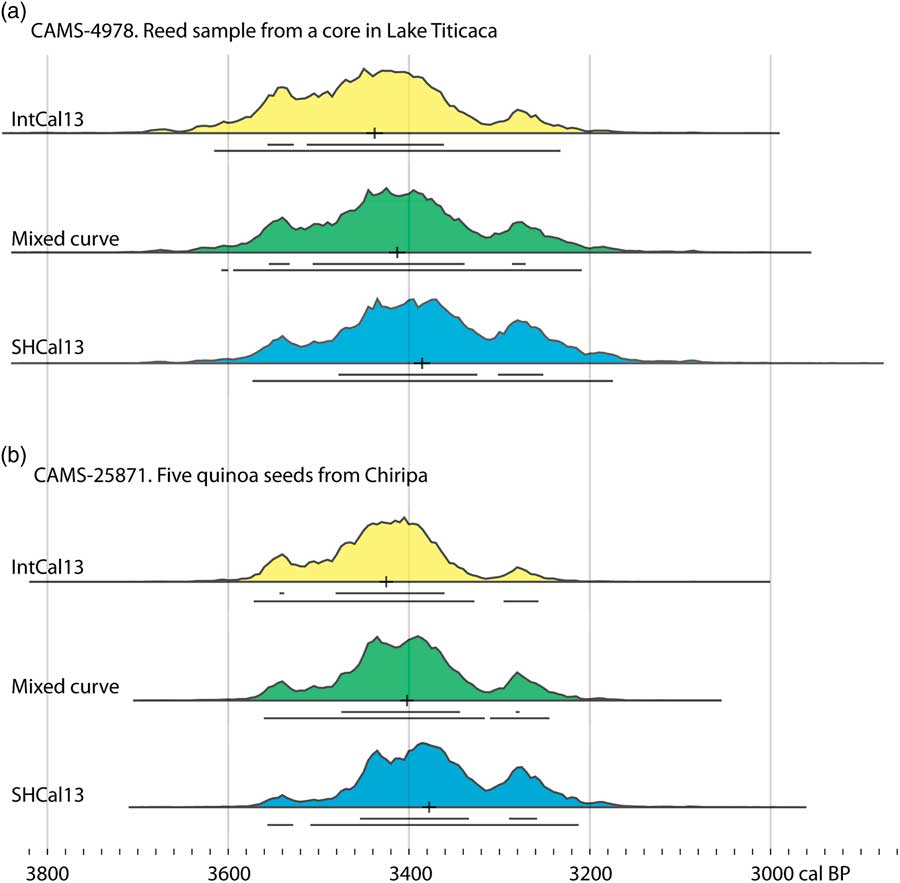
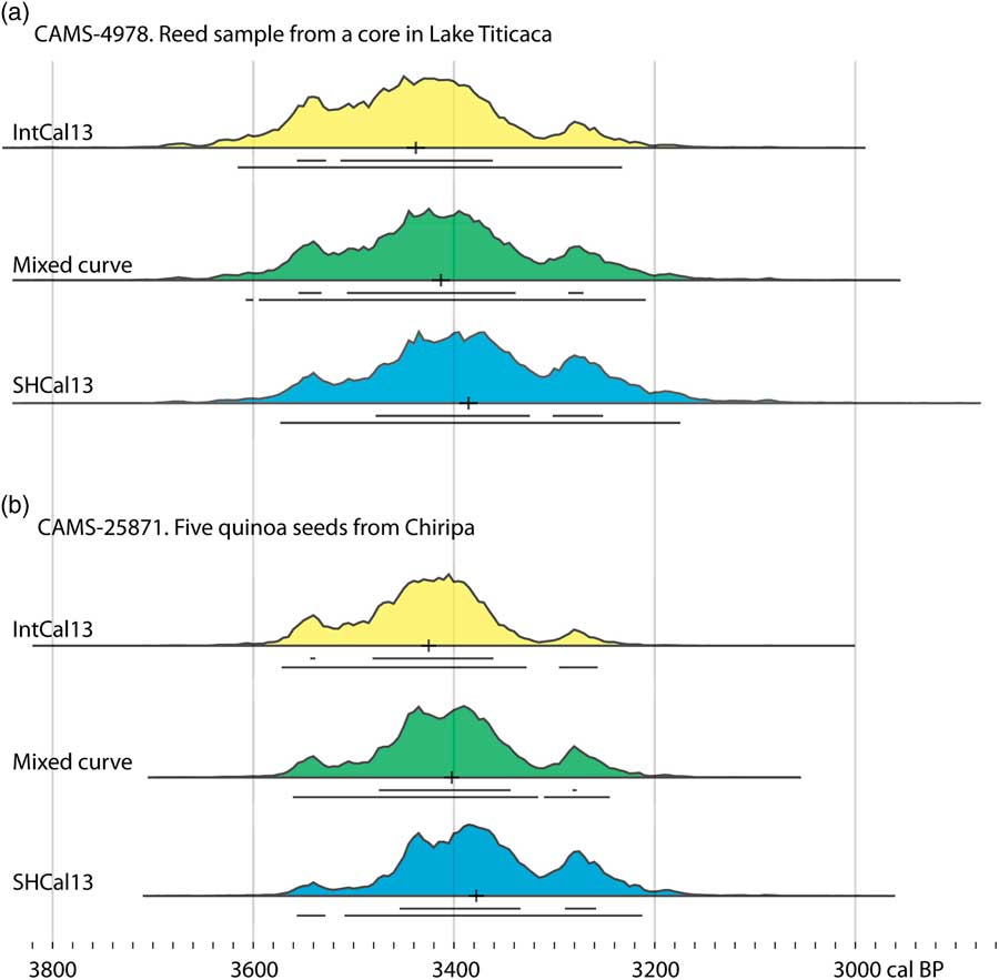
In the following example, we recalibrate one paleoclimate date and one archeological date processed at the same laboratory (Figure 5). The paleoclimate date is from a reed sample in a lake core in the southern basin of Lake Titicaca, CAMS-4978 (Abbott et al. Reference Abbott, Binford, Brenner and Kelts1997), located near an erosional surface that marks the end of mid-Holocene aridity. The archaeological date (CAMS-25871) is from the Formative site of Chiripa on the southern shore of Lake Titicaca. The sample comprises five Chenopodium seeds (from the Early Formative Santiago plaza) and is associated with domestic quinoa from one of the site’s earliest occupations (Whitehead Reference Whitehead1999; Bruno and Whitehead Reference Bruno and Whitehead2003). We used the following code in OxCal to calibrate these two dates with a mixed curve.

Figure 5

Comparison of IntCal13, mixed, and SHCal13 calibrations for (a) a paleoclimate date from a core in Lake Titicaca (CAMS-4978), which is associated with the rise of lake level, and (b) an archaeological date on Chenopodium seeds (CAMS-28571) associated with an early agropastoral occupation of the Chiripa site on the southern shore of Lake Titicaca. The horizontal lines below each curve indicate the 68% and 95% probability ranges.

Figure 5 shows the subtle differences in the shape of the probability distributions and the error ranges. At this place and span on the calibration curves, the mixed calibration has a 2–3 yr smaller error than the SHCal13 calibration. The absolute difference between the curves is quite small, so the differences between the error ranges of different curves depends on the subtle variations in the shape of both IntCal and SHCal. Both the IntCal and mixed curves show a slightly earlier mean for the end of the dry period, compared to the presence of domesticated quinoa at Chiripa. The SHCal curve means are nearly identical, and, as anticipated, slightly later. This part of the Andes is near the edge of the SASM-influenced zone in South America (Figure 4). The low-level jet that moves east over the Amazon continues to the edge of the Andes and does impact the Lake Titicaca Basin, though the degree of impact remains unclear. Thus, we would suggest that the IntCal curve is not appropriate; choosing SHCal would assume no input from the Northern Hemisphere, which remains unclear. Hence a mixed curve seems most appropriate because it makes no assumptions about the hemisphere that ¹⁴C comes from, a correct reflection of the lack of data on the impact of the SASM in the Lake Titicaca Basin. It allows for the full possible range of ¹⁴C input, from 100% Northern Hemisphere to 100% Southern Hemisphere air.

The difference between curves may seem minor in absolute terms, but for such rapid, profound changes, the sequence of events is a key element in our historical narratives and understanding of human–environment interactions. Clearly, a simplistic comparison of two calibrated dates cannot resolve this complex human–climate interaction, but we present this example to highlight the importance of refined chronologies, which must be explicit on two fronts. First paleoenvironmental and archaeological datasets must be calibrated with the same curve, and secondly, the curve choice should be based on the location of the samples. In areas with potential mixing, such as in the Lake Titicaca Basin, researchers should be explicit about the assumptions of curve choice and perhaps present multiple calibrations. Ideally, further interdisciplinary dialogue among researchers toward a consensus on the most appropriate calibration curve would facilitate future comparisons between paleoenvironmental and archaeological datasets.

FUTURE RESEARCH

Future research on tropical tree rings will undoubtedly refine our knowledge of temporal and spatial variation of atmospheric ∆¹⁴C in South America, as well as the specific areas where each calibration curve is appropriate. Specifically, these datasets could be directed at identifying potential mixtures of Northern Hemisphere air, based on wiggle-matching and Bayesian comparison to identify the most suitable curve. However, these datasets are not yet available in South America. Using extant bomb-era data, it might be more feasible to assess inter-hemispheric air mixtures during monsoon phenomena, as has been done for Thailand and Japan (Hua et al. Reference Hua, Barbetti, Zoppi, Fink, Watanasak and Jacobsen2004b; Suzuki et al. Reference Suzuki, Sakurai, Takahashi, Sato, Gunji, Tokanai, Matsuzaki and Tsuchiya2010), which could be applied in OxCal.

Additional tree-ring data could also be used to better identify the spatial boundaries of SASM influence, in addition to changes in ¹⁴C. Speleothem data, lake varves, or other similarly high-resolution and continuous records could complement detailed tree-ring chronologies. SASM influence implies seasonal variability in ¹⁴C, so future research may consider the variation in different plants’ seasonal uptake of atmospheric ¹⁴CO₂. For example, most tropical plants grow continuously throughout the year, but in some lowland areas, grasses grow during the dry season, because they are flooded during the rainy season. This issue may be relevant for tree rings used to refine ¹⁴C curves, as well as the selection of archaeological or paleoenvironmental samples for dating.

Specifically for the Altiplano, additional dates from Polylepis tarapacana tree-ring sequences (Morales et al. 2012, Reference Morales, Nielsen and Villalba2013) would be especially welcome for assessing carbon concentrations to evaluate temporal, latitudinal, and altitudinal variation in atmospheric ¹⁴C. Trends on the high-altitude Altiplano may be vey different than those in nearby tropical forests. The Altiplano is a distinctive area in terms of altitude, growth season, atmospheric influence, and long-term human impact on the environment, making it an attractive case study for refining carbon concentrations in both the air and its complex of large lacustrine basins. These lakes have significant influence on local carbon cycles and additional data are necessary to refine them (Abbott et al. Reference Abbott, Binford, Brenner and Kelts1997:172; Marsh Reference Marsh2015:16–17).

The spatial limits of SASM influence could be refined with more detailed climate modeling. Isotope backtracking is the most reliable approach for defining sources of water vapor on different parts of the continent, which could better define the area influenced by the SASM (Insel et al. Reference Insel, Poulsen, Sturm and Ehlers2013; Sturm et al. Reference Sturm, Hoffmann and Langmann2007). Such studies could be undertaken in regions where paleoclimatic and archaeological researchers work together closely, such as the Lake Titicaca Basin. In terms of global modeling, it would be timely to update Braziunas et al.’s (1995) widely cited global carbon model. It is based on differences from carbon in Seattle only (Figure 1); an updated map could compare carbon concentrations at the multiple sampled locations used to build IntCal. There are large sets of modern marine ¹⁴C data that have been mostly used to address the industrial carbon footprint (Krakauer et al. Reference Krakauer, Randerson, Primeau, Gruber and Menemenlis2006), which could also be harnessed to refine the pre-industrial latitudinal gradient of atmospheric ¹⁴C and its variability on continental scales.