




No CrossRef data available.
Article contents
THE CONTINUITY OF THE LIMIT DISTRIBUTION IN THE PARAMETER OF INTEREST IS NOT ESSENTIAL FOR THE VALIDITY OF THE BOOTSTRAP
Published online by Cambridge University Press: 24 September 2003
Abstract
It is well known that the unrestricted bootstrap estimator of the slope parameter in the random walk model without drift converges to a random distribution. This bootstrap failure is commonly attributed to the discontinuity of the limit distribution of the least-squares estimator in the parameter of interest. We demonstrate by counterexample that this type of continuity is not essential for the validity of the bootstrap nor is it essential that the rate of convergence of the estimator remain constant over the whole parameter space.We thank Don Andrews, Shinichi Sakata, Jonathan Wright, and two anonymous referees for very helpful comments. The views expressed in this paper do not necessarily reflect those of the European Central Bank or its members.
Information
- Type
- Research Article
- Information
- Copyright
- © 2003 Cambridge University Press
1. INTRODUCTION
It is well known that for certain types of statistical problems, the standard residual-based bootstrap algorithm for regression models fails. For example, consider the model

where β = 1, y0 = 0, εt is independent and identically distributed (i.i.d.) with E(εt) = 0, E(εt2) = σ2, and E(εt2+η) < ∞ for some η > 0. Basawa, Mallik, McCormick, Reeves, and Taylor (1991a) show that if α is known to be zero the unrestricted bootstrap estimator of β converges to a random distribution rather than the Dickey–Fuller (DF) limit distribution of the ordinary least-squares (OLS) estimator

. Specifically, the limiting distribution of the bootstrapped DF statistic will be a mixture with the mixing variates given by the DF limiting distribution. More precisely, the bootstrapped DF statistic has a limiting distribution similar to the DF distribution with the Brownian motion replaced by a Ornstein–Uhlenbeck process, conditional on the weak limit of

. This result generalizes to the case when an intercept is included in the regression model (see Inoue and Kilian, 2002). Note that the cause of the inconsistency of the bootstrap in this model is different from the problem discussed by Andrews (2000). Andrews (2000) focuses on bootstrapping parameters on the boundary of the parameter space. Here the parameter space is unbounded.
The bootstrap failure in model (1) stands in sharp contrast to the bootstrap validity result for stationary autoregressions (see Bose, 1988). There are several possible explanations of this failure. For example, Basawa, Mallik, McCormick, Reeves, and Taylor (1991b) attribute the bootstrap failure in model (1) to the discontinuity of the limit distribution of the OLS estimator of β at the unit circle. In their words:
The main cause of the failure of the standard bootstrap estimator at |β| = 1 … is the fact that the limit distributions of

are drastically different for the three cases: |β| < 1, |β| > 1 and |β| = 1; the point |β| = 1 serving as a threshold. This introduces instability in the bootstrap samples, which in turn leads to the eventual invalidity of the naïve bootstrap estimator at |β| = 1. (p. 1016, restated in our notation)
This intuition has been widely accepted in the econometric literature. There is a common perception that the standard residual-based algorithm for regression models will fail in the presence of a discontinuity in the limit distribution (see, e.g., Zaman, 1996, pp. 315, 316; Kilian, 1998, p. 225; Benkwitz, Lütkepohl, and Neumann, 2000, pp. 80, 82; Romano and Wolf, 2001, p. 1284).
A somewhat different and less common interpretation is provided by Benkwitz et al. (2000, p. 70), who stress that “for the bootstrap to work the convergence rate of the estimators to their asymptotic distributions must remain constant over the whole parameter space.” This is a statement not about the continuity of the limit distribution but about the constancy of the rates of convergence of the estimator.
If the intuition were correct that a discontinuity in the limit distribution of the estimator or a difference in the rate of convergence is sufficient for the bootstrap approach to fail, we would expect that the bootstrap would also fail in other circumstances when the limit distribution is discontinuous or the rates of convergence differ, such as in the random walk model (1) with α ≠ 0. Indeed, Politis, Romano, and Wolf (1999) in discussing bootstrap inference for model (1) note that
inference for β is nontrivial, because the limiting distribution of the estimator depends on the underlying parameters β and α…. If |β| < 1, the OLS estimator converges to a normal distribution at rate T1/2. For β = 1 and α = 0, it converges to a nonstandard distribution at rate T. Finally, for β = 1 and α ≠ 0, it converges to a normal distribution at rate T3/2. To construct an asymptotic confidence interval for β, it therefore seems necessary to know which the correct model is. The discontinuity of the limiting distribution causes the bootstrap (based on resampling residuals) to fail. (p. 270, restated in our notation)
The discontinuity of the rates of convergence and of the limit distribution of the slope parameter at β = 1 given α ≠ 0 may seem to suggest that the standard residual-based bootstrap method should fail in model (1) with α ≠ 0 for the same reasons that it failed in model (1) with α = 0. In this paper, we will show that this conclusion would be mistaken because continuity in this sense is not required for the asymptotic validity of the bootstrap. Specifically, we will show that the standard bootstrap approach is asymptotically valid to first order in the random walk model (1) with α ≠ 0. Note that we do not advocate this particular model for applied work. Our sole aim in this paper is to shed light on the theoretical conditions under which the bootstrap can be expected to fail. Also note that the results in this paper concern the bootstrap distribution of the unstudentized estimator of β, as opposed to the studentized estimator. Clearly, the limit distribution of the studentized estimator in model (1) with α ≠ 0 will be N(0,1) for all values of β. Because studentizing would eliminate the discontinuity of interest in this paper, we focus on the bootstrap distribution of the unstudentized estimator.
The remainder of the paper is organized as follows. In Section 2 we propose two notions of discontinuity that are consistent with the preceding quotes. We then prove by counterexample that these two notions are not related to the bootstrap failure when α = 0. In Section 3 we provide an intuitive explanation for the validity of the bootstrap in model (1) when α ≠ 0. We conclude in Section 4. The proofs can be found in the Appendix.
2. MAIN RESULT
The quotes in Section 1 suggest some ambiguity in the precise notion of discontinuity that is held responsible for the failure of the bootstrap. We begin by making more precise the notion of discontinuity. We will suggest two definitions in this section and will discuss yet another definition in Section 3. One interpretation of discontinuity that is consistent with the quotes by Basawa et al. (1991b), Zaman (1996), Benkwitz et al. (2000, pp. 80, 82), and Politis et al. (1999) is that the limit distribution is not continuous in the parameter of interest in the following sense.
DEFINITION 1 (Discontinuity of the Limit Distribution in the Parameter of Interest). Let θ denote a p-dimensional vector of parameters in the parameter space

. Consider an estimator

. Suppose that

has a nondegenerate limit distribution

where

may depend on the value of

. We say that H is discontinuous at θ if there is a sequence {θn} that converges to θ such that ρ(H(θn),H(θ)) does not converge to zero, where ρ(·,·) is some metric that metrizes weak convergence.
Note that this definition assumes that the estimator has been scaled appropriately to ensure the existence of a well-defined limit distribution. A second, somewhat different, notion of discontinuity is best described as a change in the rate of convergence of the estimator of the parameter of interest. This definition corresponds to the quote by Benkwitz et al. (2000, p. 70). It is also implicit in the emphasis on different rates of convergence in the quote by Politis et al. (1999). More formally we can state the following definition.
DEFINITION 2 (Different Rates of Convergence). Let θ denote a p-dimensional vector of parameters in the parameter space

. Consider an estimator

. Let

be a diagonal matrix of scaling factors that ensures that

has a nondegenerate limit distribution. We say that there is a discontinuity if the convergence rate of the estimator

changes over the parameter space in the sense that there are at least two different parameter values θ1 and θ2 in Θ for which the appropriate choice of

is different at θ1 and at θ2.
Note that Definition 2 is not a statement about the discontinuity of the limit distribution and hence involves a different notion of discontinuity than Definition 1. Although the two definitions are closely related, it is logically possible that an estimator is not discontinuous by Definition 1, yet the rates of convergence differ, resulting in a discontinuity according to Definition 2. Conversely, it is possible for the limit distribution to be discontinuous, even when the rates of convergence are constant across the parameter space. See Andrews (2000, pp. 401–402) and Beran (1997, p. 3) for examples.
We also note that Definitions 1 and 2 are not related to the concept of continuity used in the existing bootstrap literature. In their classical paper on the bootstrap, Bickel and Freedman (1981) provide sufficient conditions for the validity of the bootstrap for i.i.d. observations. One of their sufficient conditions is the continuity of the mapping from the distribution of observations to the limiting distribution of the statistic of interest. This concept of continuity is fundamentally different from the notion of continuity discussed in the current paper.
As the following counterexample shows, continuity in the sense of Definitions 1 and 2 is not essential for the asymptotic validity of the bootstrap. Consider an AR(1) process with drift α,

which satisfies the following set of assumptions.
Assumption 1.
(a) y0 = oas(T);
(b) εt is i.i.d. with E(εt) = 0, E(εt2) = σ2, and E(εt2+η) < ∞ for some η > 0 and is independent of y0 for t ≥ 1;
(c) the distribution of εt, F, satisfies supx|F′(x)| < ∞; and
(d) α ≠ 0.
Let

denote the OLS estimators of α and β, respectively. We are often interested in the sampling uncertainty of

. When β = 1, we know that, as noted by Dickey and Fuller (1979),

In contrast, for |β| < 1 it follows from standard results for the stationary AR(1) model (see, e.g., Hamilton, 1994, pp. 208–214) that

This result implies that the limit distribution of the OLS estimator and in particular the marginal distribution of

are discontinuous in β at β = 1 in the sense of Definition 1. We also note that at this point of discontinuity the rate of convergence changes from T1/2 to T3/2, resulting in a discontinuity in the sense of Definition 2.
We are interested in the asymptotic distribution of the corresponding bootstrap OLS estimator generated by the following bootstrap algorithm. Let

denote the residuals of the OLS estimate of process (2) given {yt}t=0T. Here

is mean zero by construction. Let

denote the empirical distribution function of

. The term

associates probability mass T−1 with

, t = 1,…,T. Treating

as the bootstrap population distribution, random samples {εt*}t=1T may be drawn from

. Thus, conditional on the data, the random variable εt* is i.i.d. with distribution function

. Now construct the bootstrap sample {yt*}t=1T recursively from

, given the initial value y0* = y0. The bootstrap estimators

then may be obtained by OLS from {yt*}t=0T.
Our analysis in this paper is nonparametric in the sense that it does not impose any parametric assumptions about the distribution of the model innovations. Although there are a number of results in the literature that establish the asymptotic validity of the bootstrap under weak assumptions (see, e.g., Beran and Ducharme, 1991), these results are based on i.i.d. resampling from a parametric distribution and hence cannot be applied directly to our example. Our results are more general in the sense of not requiring a parametric assumption but less general in the sense of being specific to a particular model.
Theorem 1 formally states our claim that the bootstrap approximation to the distribution of

remains asymptotically valid despite the discontinuity of the limit distribution of the OLS estimator and despite the change in the rate of convergence. The proof of Theorem 1 is in the Appendix.
Theorem 1. Under Assumption 1 with β = 1,

where a.s. indicates that the weak convergence holds almost surely conditional on the data.
3. DISCUSSION
It is well known that the bootstrap approximation fails for model (1) with α = 0. In contrast, Theorem 1 shows that the bootstrap approximation is valid for model (1) with α ≠ 0. One may ask why the bootstrap works in one case but not in the other. We note that this difference is not related to the fact that we use the standard nonparametric resampling scheme. Inoue and Kilian (2002) show that the bootstrap approximation fails when α = 0, even if the error distribution is known. Basawa et al. (1991a) show that the bootstrap failure occurs even when the error distribution is known to be N(0,1).
One way of developing intuition for this result is to recall that the bootstrap data-generating process is based on estimated parameters. Thus, the bootstrap data come from a model that is close to the truth but not exactly the same as the truth. This dependence on estimated parameters makes the bootstrap approximation potentially unreliable. The bootstrap can be expected to provide a valid approximation to the distribution of interest only if the estimation uncertainty associated with these parameters vanishes asymptotically. One way of ensuring that the parameter uncertainty vanishes asymptotically is ensuring local asymptotic equivalence (LAE). Beran (1997) establishes the equivalence of the validity of the bootstrap approximation and of the notion of LAE in certain settings. Although his theorems cannot be applied to model (1) with β = 1 directly, his LAE condition is useful in understanding why the bootstrap approximation works for α ≠ 0.
Specifically, Beran (1997) establishes the general validity of the bootstrap under three key conditions: LAE, local asymptotic normality, and constant rates of convergence of T1/2 across the parameter space. The last condition is violated in model (1) when α ≠ 0. Our proof involves establishing that some version of LAE holds in this case, despite the change in the rate of convergence at the unit circle. This allows us to establish the asymptotic validity of the bootstrap in this special case. In contrast, in the random walk model (1) with α = 0 the LAE condition does not hold.
Let

. Then we say that the OLS estimator

based on model (1) is LAE if, for every δ = [δ1,δ2]′ and every sequence {δT} converging to δ,

Here HT(x,θ) denotes the finite-sample distribution of the OLS estimator based on the triangular array process

where

satisfies Assumption 1. The expression H(x,θ) denotes the limit distribution of the OLS estimator that is obtained if we replace αT and βT in (6) by α and β, respectively. Note that H(x,θ) does not depend on δ. Let

denote the OLS estimator based on (6). When α ≠ 0, it follows from equation (A.6) in the Appendix that

In this case, LAE holds because the deterministic trend in yT,t dominates the stochastic trend in yT,t as in the well-known case of δ = [0,0]′. In contrast, when α = 0, under Assumption 1 with Assumption 1(a) replaced by y0 = oas(T1/2) one can show that

where {W(s) : 0 ≤ s ≤ 1} is a standard Brownian motion and

For completeness, we provide the proof of (8) in the Appendix. In this case, LAE does not hold because the limit distribution depends on δ.
Note that the conditions we provide—like the conditions provided by Beran (1997)—are sufficient, but not necessary for the asymptotic validity of the bootstrap. To date no set of necessary conditions exists for the type of problem addressed in this paper. Although we are unable to isolate the root cause of the failure of the bootstrap in the random walk model without drift, our analysis shows that one condition that may have seemed necessary for the validity of the bootstrap—namely, continuity in the sense of Definitions 1 and 2—is in fact not necessary.
A referee pointed out that perhaps the notion of discontinuity that Basawa et al. (1991b) and Politis et al. (1999) had in mind is different from Definition 1 and proposed an alternative definition, which follows.
DEFINITION 3 (Discontinuity in the Type of Limit Distribution). Let θ denote a p-dimensional vector of parameters in the parameter space

. Consider an estimator

of θ. Suppose that

has a nondegenerate limit distribution H(x,θ) where

may depend on the value of θ. We say that there is a discontinuity if the parametric family of H(x,θ) changes over the parameter space (say, from Gaussian for θ1 to non-Gaussian for θ2).
Note that a discontinuity in the sense of Definition 3 implies a discontinuity in the sense of Definition 1 but not a discontinuity in the sense of Definition 2. According to Definition 3, there is a discontinuity in the case when α = 0 because at the unit circle the type of distribution changes from Gaussian to Dickey–Fuller, but there is no discontinuity when α ≠ 0 because the distribution remains Gaussian even at the unit circle. This is consistent with the bootstrap failure in the first, but not in the second, case. To the extent that Politis et al. (1999) predicted that the bootstrap would fail for model (1) with α ≠ 0, whereas the use of Definition 3 suggests otherwise, it would seem obvious that Politis et al. clearly did not have Definition 3 in mind but rather Definition 1 or 2. On the other hand, the Basawa et al. (1991b) quote is potentially consistent with Definition 3, as are statements by Romano and Wolf (2001, pp. 1283, 1286) that refer to changes in the “form” or in the “type” of the limit distribution in the context of the random walk model with α = 0. The latter paper also explicitly refers to Definition 2 in the same sentence, however. Thus, the extent to which Definition 3 has been appealed to in the literature is unclear.
Does the absence of a discontinuity in the sense of Definition 3 explain the success of the bootstrap in the random walk model with α ≠ 0? Although this hypothesis seems to fit the facts in this case, there does not appear to be any obvious relationship between Definition 3 and the technical conditions underlying Theorem 1. Notably, there is no straightforward relationship between LAE and the absence of a discontinuity in the sense of Definition 3. The former is a statement about the convergence of the finite-sample distribution of the estimator at a local parameter value to the limit distribution of the estimator at the population parameter. The latter is a statement about the limit distribution itself. Thus, the practical usefulness of Definition 3 is open to question. Moreover, it is clear that the absence of a discontinuity in the sense of Definition 3 is not enough for the bootstrap to be valid. For example, the Hodges estimator is asymptotically normally distributed for all parameter values (and hence continuous in the relevant sense), but its bootstrap approximation fails (see, e.g., Beran, 1997). This leaves the possibility that the presence of a discontinuity in the sense of Definition 3 may be sufficient for the bootstrap to fail. We were unable to disprove this proposition by counterexample. Establishing such a relationship, if it exists, would be a useful exercise.
4. CONCLUSION
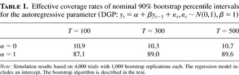
We conclude with an illustration of the implications of our theoretical results for bootstrap inference in finite samples. We evaluate the coverage accuracy of nominal 90% bootstrap percentile confidence intervals for

in the random walk model with and without drift. The percentile intervals are constructed by inverting the 5% and 95% quantiles of the empirical distribution of the bootstrap estimator

and do not require any knowledge of the rate of convergence of the estimator or its variance (see Efron and Tibshirani, 1993). The results are shown in Table 1. Consider the case of α = 0 and β = 1. For T = 100, the coverage rate is only 11%. There is no improvement in coverage accuracy as T increases to 300 and 500. In contrast, for the case of α = 1 and β = 1, the coverage accuracy of the interval is 87% for T = 100 and improves to 89% for T = 300 and 90% for T = 500.
Effective coverage rates of nominal 90% bootstrap percentile intervals for the autoregressive parameter (DGP: yt = α + βyt−1 + εt,εt ∼ N(0,1),β = 1)

These results suggest that the theory presented is useful for understanding the finite-sample behavior of the estimator of β in the AR(1) model. They do not, of course, provide any practical guidance because in practice we would not know whether α = 0 or not. Moreover, if α ≠ 0 and if we wish to allow for the possibility that β = 1, it would be common practice to include a linear time trend, in which case the bootstrap approximation would fail in the presence of a unit root (see Inoue and Kilian, 2002).
Rather than providing advice to applied researchers the aim of this paper has been to improve our understanding of when the bootstrap does and does not work. We observed that it is common to associate the failure of the bootstrap in the random walk model without drift with a discontinuity at the unit circle. We called attention to the fact that there apparently exist quite different notions of discontinuity in the literature. We showed that it is important to be precise about the notion of discontinuity involved and to be explicit about the link from discontinuity to bootstrap invalidity. Specifically, our analysis demonstrated that the continuity of the limit distribution of the estimator in the parameter of interest is not essential for the success of the bootstrap. Nor is it essential that the rates of convergence of the estimators to their asymptotic distributions remain constant over the whole parameter space. Our analysis establishes that these notions of continuity are not among the necessary conditions for the validity of the bootstrap.
APPENDIX
Proof of Theorem 1. We adopt the following additional notation. Let

denote the weak convergence of probability measures and [x] denote the integer part of x. The term I(·) is the indicator function. Let

denote the space of probability measures on X topologized by weak convergence. Given an m × n matrix A = {aij}, let

. For

be the infimum of (E∥X − Y ∥r)1/r, over all possible joint distributions of two random vectors X and Y whose marginal distributions are μ and ν, respectively. The notation LX,Y stands for the joint distribution of X and Y, a ∧ b stands for the minimum of a and b, and a ∨ b denotes the maximum of a and b.
First, consider the data-generating process with the parameters deterministically converging to (α,1) ≠ (0,1) as T → ∞. Specifically we consider the triangular array

where

is the Pitman drift parameter, yT,0 = y0, and εt satisfies Assumption 1. Expression (A.1) is similar to the bootstrap data generating process, except that in the bootstrap world OLS estimates will take the place of the deterministic sequence [αT,βT]′ in (A.1). By repeated substitution, we obtain

Let [z] denote the integer part of z. Then it follows that, for r ∈ [0,1] ,

where Op is uniform in r.
Thus it follows from the functional central limit theorem and the continuous mapping theorem that

and

Let

denote the OLS estimator based on the triangular array (A.1). From (A.4) and (A.5) it follows that

Next, we shall derive the limiting distribution of the bootstrap OLS estimator when αT and βT in (A.1) are replaced with their OLS estimates

. Let G denote the distribution of the right-hand side (RHS) of (A.6) and

where P* is the probability measure induced by the bootstrap conditional on the original data,

. We will show that, as T → ∞,

The term GT(·) is not a function of

alone but is also a function of

, and thus it is difficult to prove (A.7) directly. To circumvent this difficulty, we follow a two-step procedure. First, consider a thought experiment, in which we bootstrap the regression parameters under the counterfactual assumption that the true error distribution is known, i.e.,

where

. The bootstrap analogue of GT under this resampling scheme is given by

where

. Second, consider the standard bootstrap resampling scheme

where

.
Let

. We will proceed as follows. First, in Lemma 1 we will provide bounds for the difference between

and between

. We show that this difference vanishes asymptotically for

close to unity. This fact allows us to substitute

for UT* and VT*, respectively, and to proceed as though F were known. Thus, in the subsequent analysis we can treat

, respectively, as interchangeable. Second, in Lemma 2, we will prove that the distance between the bootstrap innovation and the true innovation vanishes asymptotically. This result will be used in proving Lemma 3. Third, in Lemma 3, we will derive the limit distribution of UT* and VT*. Finally, we will apply the continuous mapping theorem to show that VT*−1UT* indeed converges to the limit distribution of the bootstrap estimator.
LEMMA 1. The following three statements are true:


Proof of Lemma 1. Following Datta (1996) and Inoue and Kilian (2002), assume that

. We first verify expression (A.9). Because


it follows that

Similarly, because

we obtain that

Because

expression (A.9) follows from (A.14) and (A.15).
Next we will derive expression (A.10) along similar lines. It follows from (A.12) and (A.13) that

Thus we have

Because

(A.10) follows from (A.19).
Expression (A.11) follows immediately from (A.9) and (A.10). █
In the rest of the proof, we treat

as

-valued random elements, where M2×2 is a set of 2 × 2 real matrices. Lemma 2 shows that the distance between the bootstrap innovation and the population innovation vanishes asymptotically. This result will be used in the proof of Lemma 3.
LEMMA 2.

Proof of Lemma 2. By Lemma 8.3(a) of Bickel and Freedman (1981), (A.21) holds if

and if

We will verify both conditions, starting with condition (A.23). Observe that by the strong law of large numbers

Thus, it only remains to be shown that

holds. It follows from the definition of yt−1 and the law of the iterated logarithm that


and

It follows from (A.26), (A.27), and (A.28) that


By combining (A.29) and (A.30) we obtain (A.25).
Next, we will verify condition (A.22). As shown by Billingsley (1968, pp. 17–18), it suffices to prove that

for all

. Note that by definition

where

. Note that the first term on the RHS of (A.32) is o(1) a.s. by the strong law of large numbers. By Assumption 1(c), there is a finite positive number MF such that |F(x′) − F(x)| < MF|x′ − x| for all x,x′. Hence,

where the last equality follows from (A.26), (A.29), and (A.30). Thus, the second term on the RHS of (A.32) is o(1) a.s. Next, we will show that the third term on the RHS of (A.32) is o(1) a.s., i.e.,

It follows from (A.29) and (A.30) that

In other words, there is a finite positive number M such that

for

Let Δt = maxb∈BM b′xt and Δt = minb∈BM b′xt. Then

We will show that the left part of the inequality (A.36) is o(1) a.s. The proof that the right part of (A.36) is o(1) a.s. is analogous and thus is omitted. If the left and right parts of (A.36) are o(1) a.s., the expression in the middle of the inequality is o(1) a.s., and thus (A.31) holds.
By construction, ht = {I(εt ≤ x + Δt) − F(x + Δt) − I(εt ≤ x) + F(x)} is a martingale difference sequence. Thus, by the Chebyshev inequality,

It follows from (A.29) and (A.30) that

Thus,

By the Borel–Cantelli lemma, it follows that

By (A.29) and (A.30),

Thus, the left part of the inequality (A.36) is o(1) a.s. Therefore, (A.31) holds, and hence so does condition (A.22). █
LEMMA 3. Let U and V be the RHS of (A.4) and (A.5), respectively. Then

Proof of Lemma 3. Because LUT*,VT* and LU,V are

-valued random elements and

is separable, by Theorems 6.2 and 6.6 of Parthasarathy (1967), it is sufficient to prove

for every bounded uniformly continuous function g on

.

where Mg is a bound for g and K is a real number. Because

, the second term can be made arbitrarily small by choosing a sufficiently large K. On the set

by Lemmas 1 and 2, and thus

by Theorem II 6.6 in Parthasarathy (1967). Because g is uniformly continuous and bounded, the first term converges to zero by the dominated convergence theorem. Thus,

It follows from (3) and the Skorohod representation theorem that there are

such that

denotes the random vector on the RHS of (3). Let

correspond to

, respectively, with

replaced by

, respectively. Let

correspond to U and V, respectively, with

replaced by

. By Lemma 1,

Because by the Skorohod representation theorem

, it follows from (A.46) that

by the dominated convergence theorem. █
Because UT* and VT* correspond to the numerator and the denominator of the limiting expression of the bootstrap estimator in (5), the continuous mapping theorem completes the proof of Theorem 1. █
Proof of (8). Because

(for the latter, see Phillips, 1987), it follows from (A.2) and (αT,βT) = (δ1T−1/2,1 + δ2T−1) that

where Jδ(r) is defined after equation (8). Note that the second term in the definition of (8) is an Ornstein–Uhlenbeck process. Thus, applications of Lemma 1 of Phillips (1987) yield the desired result. █
References
REFERENCES
Andrews, D.W.K.
(2000)
Inconsistency of the bootstrap when a parameter is on the boundary
of the parameter space.
Econometrica
68,
399–405.Google Scholar
Basawa, I.V.,
A.K. Mallik,
W.P. McCormick,
J.H. Reeves, &
R.L. Taylor
(1991a)
Bootstrapping unstable first-order autoregressive processes.
Annals of Statistics
19,
1098–1101.Google Scholar
Basawa, I.V.,
A.K. Mallik,
W.P. McCormick,
J.H. Reeves, &
R.L. Taylor
(1991b)
Bootstrap test of significance and sequential bootstrap estimation
for unstable first-order autoregressive processes.
Communications in Statistical Theory and Methods
20,
1015–1026.Google Scholar
Benkwitz, A.,
H. Lütkepohl, &
M.H. Neumann
(2000)
Problems related to confidence intervals for impulse responses of
autoregressive processes.
Econometric Reviews
19,
69–103.Google Scholar
Beran, R.
(1997)
Diagnosing bootstrap success.
Annals of the Institute of Statistical Mathematics
49,
1–24.Google Scholar
Beran, R. &
G.R. Ducharme
(1991)
Asymptotic Theory for Bootstrap Methods in Statistics.
Les Publications CRM, Centre de recherches mathematiques.
Montreal:
University of Montreal.
Bickel, P.J. &
D.A. Freedman
(1981)
Some asymptotic theory for the bootstrap.
Annals of Statistics
9,
1196–1217.Google Scholar
Billingsley, P.
(1968)
Convergence of Probability Measures.
New York:
Wiley.
Bose, A.
(1988)
Edgeworth correction by bootstrap in autoregression.
Annals of Statistics
16,
1709–1722.Google Scholar
Datta, S.
(1996)
On asymptotic properties of bootstrap for AR(1) processes.
Journal of Statistical Planning and Inference
53,
361–374.Google Scholar
Dickey, D.A. &
W.A. Fuller
(1979)
Distribution of the estimators for autoregressive time series with
a unit root.
Journal of the American Statistical Association
74,
427–431.Google Scholar
Efron, B. &
R.J. Tibshirani
(1993)
An Introduction to the Bootstrap.
New York:
Chapman and Hall.
Hamilton, J.D.
(1994)
Time Series Analysis.
Princeton:
Princeton University Press.
Inoue, A. &
L. Kilian
(2002)
Bootstrapping autoregressions with possible unit roots.
Econometrica
70,
377–391.Google Scholar
Kilian, L.
(1998)
Small-sample confidence intervals for impulse response functions.
Review of Economics and Statistics
80,
218–230.Google Scholar
Parthasarathy, K.R.
(1967)
Probability Measures on Metric Spaces.
New York:
Academic Press.
Phillips, P.C.B.
(1987)
Towards a unified asymptotic theory for autoregression.
Biometrika
74,
535–547.Google Scholar
Politis, D.N.,
J.P. Romano, &
M. Wolf
(1999)
Subsampling.
New York:
Springer-Verlag.
Romano, J.P &
M. Wolf
(2001)
Subsampling intervals in autoregressive models with linear time
trend.
Econometrica
69,
1283–1314.Google Scholar
Zaman, A.
(1996)
Statistical Foundations for Econometric Techniques.
San Diego:
Academic Press.
Effective coverage rates of nominal 90% bootstrap percentile intervals for the autoregressive parameter (DGP: yt = α + βyt−1 + εt,εt ∼ N(0,1),β = 1)
 You have
Access
- 7
- Cited by