1. Introduction
Over the past 60 years, the axisymmetric turbulent wake has been extensively studied experimentally and numerically (see e.g. Johansson, George & Gourlay Reference Johansson, George and Gourlay2003; Brown & Roshko Reference Brown and Roshko2012, for historical reviews). A basic problem of particular interest is the scaling with streamwise distance
 $x$
of the wake width
 ${\it\delta}$
and the centreline velocity deficit
 $u_{0}$
(Tennekes & Lumley Reference Tennekes and Lumley1972; Townsend Reference Townsend1976; Bevilaqua & Lykoudis Reference Bevilaqua and Lykoudis1978; George Reference George, George and Arndt1989). As stated in Johansson et al. (Reference Johansson, George and Gourlay2003), this problem ‘has puzzled researchers for more than a half-century since measured results have been either inconclusive or contradictive’. The equilibrium similarity analysis of George (Reference George, George and Arndt1989) has shown that two scalings are possible for the streamwise evolutions of the wake width and the velocity deficit. The classical equilibrium high-Reynolds-number scaling is obtained by assuming, as in Townsend (Reference Townsend1976) and George (Reference George, George and Arndt1989), that the turbulence dissipation rate
 ${\it\varepsilon}$
scales as
 ${\it\varepsilon}=C_{{\it\varepsilon}}K^{3/2}/{\it\delta}$
, where
 $C_{{\it\varepsilon}}=\text{const.}$
and
 $K$
is the turbulent kinetic energy. This leads to the high-Reynolds-number scalings
 $$\begin{eqnarray}\displaystyle & \displaystyle \frac{u_{0}(x)}{U_{\infty }}\sim \left(\frac{x-x_{0}}{{\it\theta}}\right)^{-2/3}, & \displaystyle\end{eqnarray}$$
 $$\begin{eqnarray}\displaystyle & \displaystyle \frac{{\it\delta}(x)}{{\it\theta}}\sim \left(\frac{x-x_{0}}{{\it\theta}}\right)^{1/3}, & \displaystyle\end{eqnarray}$$
 $U_{\infty }$
is the free-stream velocity,
 ${\it\theta}$
is the momentum thickness and
 $x_{0}$
is a virtual origin, which comes out naturally from the analysis. George (Reference George, George and Arndt1989) (see also Johansson et al.
Reference Johansson, George and Gourlay2003) has shown that another, different, scaling is present when the viscous term in the mean momentum equation is not negligible. This is a low-Reynolds-number regime for which
 ${\it\varepsilon}\sim {\it\nu}K/{\it\delta}^{2}$
, where
 ${\it\nu}$
is the kinematic viscosity of the fluid. These low-Reynolds-number scalings are
 $$\begin{eqnarray}\displaystyle & \displaystyle \frac{u_{0}(x)}{U_{\infty }}\sim \mathit{Re}_{G}\left(\frac{x-x_{0}}{{\it\theta}}\right)^{-1}\left(\frac{{\it\theta}}{L_{b}}\right), & \displaystyle\end{eqnarray}$$
 $$\begin{eqnarray}\displaystyle & \displaystyle \frac{{\it\delta}(x)}{{\it\theta}}\sim \mathit{Re}_{G}^{-1/2}\left(\frac{x-x_{0}}{{\it\theta}}\right)^{1/2}\left(\frac{L_{b}}{{\it\theta}}\right)^{1/2}, & \displaystyle\end{eqnarray}$$
 $\mathit{Re}_{G}$
is a global Reynolds number determined by the inlet conditions and
 $L_{b}$
is a reference length scale characterising the wake generator. The low-Reynolds-number regime has only been observed at very large distances from the wake generator by Johansson et al. (Reference Johansson, George and Gourlay2003), who found it in the temporally evolving wake simulation data of Gourlay et al. (Reference Gourlay, Arendt, Fritts and Werne2001). However, no transition to this regime has been observed in the recent work of Redford, Castro & Coleman (Reference Redford, Castro and Coleman2012), where the classical high-Reynolds-number scalings were recovered for very long times in their temporally evolving simulations (equivalent to very long streamwise distances). Note, however, that one of the simulations of Redford et al. (Reference Redford, Castro and Coleman2012) did return the scalings
 $u_{0}(x)/U_{\infty }\sim x^{-1}$
and
 ${\it\delta}(x)/{\it\theta}\sim x^{1/2}$
, but at higher local Reynolds numbers and earlier times than those where the classical predictions (1.1) and (1.2) appear.
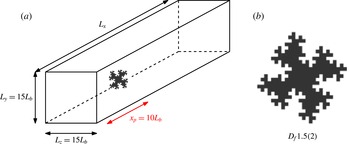
Schematic view of the flow configuration (a) and drawing of the irregular plate used to generate a turbulent wake (b).

Recently, Nedić, Ganapathisubramani & Vassilicos (Reference Nedić, Ganapathisubramani and Vassilicos2013a ) and Nedić, Vassilicos & Ganapathisubramani (Reference Nedić, Vassilicos and Ganapathisubramani2013b ) used non-axisymmetric plates with irregular edges (see figure 1) and showed that the turbulent wakes they generate when placed normal to a free stream is at least as axisymmetric as turbulent wakes generated by axisymmetric disks. These multiscale wake generators combine wake-like with jet-like behaviours, and their turbulent wakes obey wake laws that are different from the usual axisymmetric turbulent wake laws. Nedić et al. (Reference Nedić, Vassilicos and Ganapathisubramani2013b ) have argued that these new scaling laws for the wake width and centreline velocity deficit can be explained in terms of the similarity analysis for axisymmetric wakes of George (Reference George, George and Arndt1989) and are as follows:
 $$\begin{eqnarray}\displaystyle & \displaystyle \frac{u_{0}(x)}{U_{\infty }}\sim \left(\frac{x-x_{0}}{{\it\theta}}\right)^{-2/(3-n)}\mathit{Re}_{G}^{2(n-m)/(3-n)}\left(\frac{L_{b}}{{\it\theta}}\right)^{-2n/(3-n)}, & \displaystyle\end{eqnarray}$$
 $$\begin{eqnarray}\displaystyle & \displaystyle \frac{{\it\delta}(x)}{{\it\theta}}\sim \left(\frac{x-x_{0}}{{\it\theta}}\right)^{1/(3-n)}\mathit{Re}_{G}^{(m-n)/(3-n)}\left(\frac{L_{b}}{{\it\theta}}\right)^{-n/(3-n)}, & \displaystyle\end{eqnarray}$$
 $m$
and
 $n$
is caused by the assumption made on the turbulence dissipation scaling. Indeed, these new wake laws are direct consequences of the assumed non-equilibrium dissipation law (see Vassilicos Reference Vassilicos2015)
 $$\begin{eqnarray}{\it\varepsilon}=C_{{\it\varepsilon}}\frac{K^{3/2}}{{\it\delta}}\quad \text{with }C_{{\it\varepsilon}}\sim \frac{\mathit{Re}_{G}^{m}}{\mathit{Re}_{l}^{n}},\end{eqnarray}$$
where
 $\mathit{Re}_{l}$
is a local Reynolds number based on local velocity and length scales. As reported in Vassilicos (Reference Vassilicos2015), the values of
 $m$
and
 $n$
in the non-equilibrium high-Reynolds-number region of grid-generated turbulence are
 $m\approx 1\approx n$
.
Adopting
 $n=m=1$
for axisymmetric turbulent wakes, the scaling laws (1.5) and (1.6) become
 $$\begin{eqnarray}\displaystyle & \displaystyle \frac{u_{0}(x)}{U_{\infty }}\sim \left(\frac{x-x_{0}}{{\it\theta}}\right)^{-1}\left(\frac{{\it\theta}}{L_{b}}\right), & \displaystyle\end{eqnarray}$$
 $$\begin{eqnarray}\displaystyle & \displaystyle \frac{{\it\delta}(x)}{{\it\theta}}\sim \left(\frac{x-x_{0}}{{\it\theta}}\right)^{1/2}\left(\frac{L_{b}}{{\it\theta}}\right)^{1/2}. & \displaystyle\end{eqnarray}$$
The main purpose of this paper is to use direct numerical simulation (DNS) and hot-wire anemometry (HWA) measurements of axisymmetric turbulent wakes of a fractal/multiscale-edge plate placed normal to the incoming flow to carefully establish each one of the assumptions leading to the predictions such as (1.5) and (1.6) and in particular the existence of the new non-equilibrium dissipation law (1.7). The very significant advantage of fractal/multiscale-edge plates for wind tunnel experiments of turbulent wakes is that they produce much higher local Reynolds numbers than regular-edge plates with the same surface area. This way the plate’s surface can be chosen small enough for the streamwise extent over which the wake is measured to be as long as possible without the velocity deficit dropping to values so low that HWA measurements become too challenging. A low-surface-area plate also imposes a low blockage in the wind tunnel, which is also an advantage.
We start with a detailed DNS assessment of the boundary layer approximation of the mean momentum equation. The axisymmetry and self-similarity/self-preservation properties of the flow are then examined both experimentally and computationally. Finally, the streamwise evolution and scalings of the turbulence dissipation rate are studied with both DNS and HWA, leading to a study of the consistency between the velocity deficit and wake width scalings and the non-equilibrium dissipation law.
The flow configuration is described in § 2. The numerical methods are described in § 3 and the experimental set-up in § 4. The leading and the negligible terms in the Reynolds-averaged momentum balance are established in § 5 and the axisymmetry of the flow is established in § 6. The self-similarity properties of mean profiles are analysed in § 7 and the new dissipation law (1.7) is discussed in § 8. In § 9 we develop a revised approach to the prediction of the wake width and velocity deficit, which we compare with our numerical and experimental data. Finally, the main results are summarised in § 10.
2. Flow configuration
In the present study, turbulent wakes are generated by a bluff plate of surface area
 $A$
with irregular edge periphery (allowing the formation of jet-wake flows) placed normal to the laminar free stream (see figure 1
b). This irregular plate is the same as one of those used in Nedić et al. (Reference Nedić, Vassilicos and Ganapathisubramani2013b
). The perimeter shape of this plate results from a geometric self-similar process, leading, if continued ad infinitum, to a plate with fractal perimeter of infinite length and fractal dimension
 $D_{f}=1.5$
but the same surface area
 $A$
. A schematic view of the generic flow configuration considered in both the experiments and the DNS is presented in figure 1(a). In the Cartesian coordinate system
 $(O;x,y,z)$
, the domain is
 ${\it\Omega}=[-x_{p},L_{x}-x_{p}]\times [-L_{y}/2,L_{y}/2]\times [-L_{z}/2,L_{z}/2]$
, where
 $x_{p}$
is the longitudinal location of the plate and the origin
 $O$
is located at the centre of the plate. The reference length
 $L_{b}$
of the flow is defined by
 $L_{b}=\sqrt{A}$
. For the sake of simplicity, the radial distance
 $r=\sqrt{y^{2}+z^{2}}$
and the polar angle
 ${\it\varphi}=\arctan (y/z)$
are also introduced hereinafter. The lateral dimensions of the domain
 $L_{y}$
and
 $L_{z}$
are the same for the wind tunnel experiments and the DNS, with
 $L_{y}=L_{z}=15L_{b}$
. However, the streamwise dimension considered for the DNS is twice the length of the wind tunnel’s test section, with
 $L_{x}^{DNS}=2L_{x}^{HWA}=120L_{b}$
. Because the plate is located at
 $x_{p}=10L_{b}$
in both cases, the measurements are taken up to
 $x=50L_{b}$
for the experiments and
 $x=110L_{b}$
for the DNS. In the DNS case, results are reported in the range
 $x\in [5L_{b};100L_{b}]$
to avoid spurious effects due to the outflow boundary conditions. The boundaries of the domain are: (i) the flow inlet at
 $x=-x_{p}=-10L_{b}$
; (ii) the lateral boundaries at
 $y=\pm L_{y}/2$
and
 $z=\pm L_{z}/2$
; and (iii) the outlet at
 $x=L_{x}-x_{p}$
.
In the DNS case, mean quantities
 $\langle \,f\rangle _{{\it\varphi},t}(x,r)$
of a field
 $f(x,r,{\it\varphi},t)$
are estimated by averaging over time and over the homogeneous polar direction
 ${\it\varphi}$
in the cylindrical coordinate system
 $(x,r,{\it\varphi})$
. In the case of the HWA measurements, the mean quantity
 $\langle \,f\rangle _{t}(x,r)$
is estimated by averaging over time only. For simplicity, both notations are replaced by
 $\langle \,f\rangle (x,r)$
in this paper, the context making the detailed meaning of the notation clear. The mean streamwise velocity component
 $\langle u_{x}\rangle (x,r)$
is denoted
 $U$
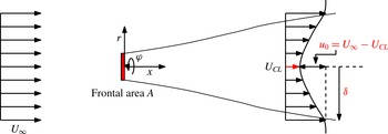
. A schematic view of the axisymmetric wake is presented in figure 2 with some definitions. The momentum thickness is defined by
 $$\begin{eqnarray}{\it\theta}^{2}=\frac{1}{U_{\infty }^{2}}\int _{0}^{\infty }U_{\infty }(U_{\infty }-U)r\,\text{d}r=\text{const.},\end{eqnarray}$$
and the wake’s width is here characterised by the integral wake’s width,
 $$\begin{eqnarray}{\it\delta}^{2}(x)=\frac{1}{u_{0}}\int _{0}^{\infty }(U_{\infty }-U)r\,\text{d}r,\end{eqnarray}$$
where
 $u_{0}(x)=U_{\infty }-U(x,r/L_{b}=0)$
is the centreline velocity deficit. To be unambiguous, these definitions rely on axisymmetry in the HWA case. To avoid negative values of the velocity deficit
 $U_{\infty }-U$
due to the finite size of the domain, a local free-stream velocity
 $U_{\infty }=U(x,R)$
is used in these definitions, where
 $R=5L_{b}$
is the maximum radial location considered for the DNS. For the experiments,
 $U_{\infty }$
is taken to be the maximum value of the mean velocity profile at each streamwise location, i.e.
 $U_{\infty }=\max _{r}(U)$
.
Axisymmetric wake coordinates and definitions.

The global Reynolds number
 $\mathit{Re}_{G}$
of the flow is based on the reference length
 $L_{b}=\sqrt{A}$
and the free-stream velocity
 $U_{\infty }$
,
 $$\begin{eqnarray}\mathit{Re}_{G}=\frac{U_{\infty }L_{b}}{{\it\nu}},\end{eqnarray}$$
where
 ${\it\nu}$
is the (constant) kinematic viscosity. The local Reynolds number
 $\mathit{Re}_{l}$
is defined by
 $$\begin{eqnarray}\mathit{Re}_{l}=\frac{\sqrt{K_{0}}{\it\delta}}{{\it\nu}},\end{eqnarray}$$
where
 $K_{0}$
is the turbulent kinetic energy at a centreline location.
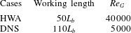
Two cases, summarised in table 1, are considered in the present study. The HWA case refers to experiments carried out at
 $\mathit{Re}_{G}=40\,000$
and the DNS case to a numerical simulation performed in a similar flow configuration but at
 $\mathit{Re}_{G}=5000$
because of the highly demanding computations of the present DNS.
Summary of the two different cases considered in this study.

To conclude this section, and for illustrative purposes only, an instantaneous visualisation of the turbulent wake generated by the DNS is plotted in figure 3 for a streamwise range corresponding approximately to the length of the experimental test section.
Instantaneous visualisation of an isosurface of vorticity magnitude
 $\Vert {\it\omega}\Vert =2$
for the DNS simulation. The streamwise range plotted here is from
 $x=5L_{b}$
to
 $x=45L_{b}$
corresponding approximately to the experimental work section.

3. Numerical methods
The finite difference code ‘Incompact3d’ (Laizet & Lamballais Reference Laizet and Lamballais2009; Laizet, Lamballais & Vassilicos Reference Laizet, Lamballais and Vassilicos2010) is used to solve the incompressible Navier–Stokes equations
 $$\begin{eqnarray}\displaystyle & \displaystyle \frac{\partial \boldsymbol{u}}{\partial t}+\frac{1}{2}(\boldsymbol{{\rm\nabla}}\boldsymbol{\cdot }(\boldsymbol{u}\otimes \boldsymbol{u})+(\boldsymbol{u}\boldsymbol{\cdot }\boldsymbol{{\rm\nabla}})\boldsymbol{u})=-\frac{1}{{\it\rho}}\boldsymbol{{\rm\nabla}}p+{\it\nu}{\rm\Delta}\boldsymbol{u}+\boldsymbol{f}, & \displaystyle\end{eqnarray}$$
 $$\begin{eqnarray}\displaystyle & \boldsymbol{{\rm\nabla}}\boldsymbol{\cdot }\boldsymbol{u}=0, & \displaystyle\end{eqnarray}$$
 $\boldsymbol{u}=(u_{x},u_{y},u_{z})^{\text{T}}$
is the velocity,
 $p$
the pressure and
 ${\it\rho}$
(constant) the density of the fluid. The convective terms are written in the skew-symmetric form to enable reduction in aliasing errors and improvement of kinetic energy conservation for the spatial discretisation used in the code (Kravchenko & Moin Reference Kravchenko and Moin1997). The modelling of the plate is performed by an immersed boundary method, following a procedure proposed by Parnaudeau et al. (Reference Parnaudeau, Carlier, Heitz and Lamballais2008). The present method is a direct forcing approach that ensures the zero-velocity boundary condition at the plate walls. It mimics the effects of a solid surface on the fluid via the additional forcing term
 $\boldsymbol{f}$
in the Navier–Stokes equations. Inflow/outflow boundary conditions are assumed in the streamwise direction with a uniform fluid velocity
 $U_{\infty }$
without turbulence as inflow condition and a one-dimensional convection equation as outflow condition. The boundary conditions in the two spanwise directions are periodic. The computational domain
 $L_{x}\times L_{y}\times L_{z}=120L_{b}\times 15L_{b}\times 15L_{b}$
is discretised on a Cartesian grid of
 $n_{x}\times n_{y}\times n_{z}=3841\times 480\times 480$
points. In terms of Kolmogorov microscale
 ${\it\eta}$
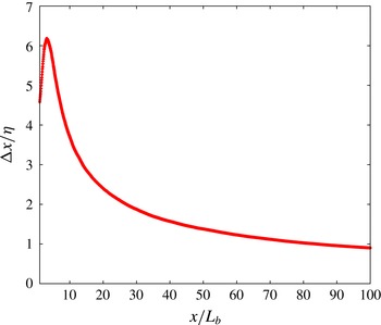
, as illustrated in figure 4, the spatial resolution is at worst
 ${\rm\Delta}x={\rm\Delta}y={\rm\Delta}z\approx 6{\it\eta}$
(where the turbulence is at its most intense) and at best
 ${\rm\Delta}x={\rm\Delta}y={\rm\Delta}z\approx 0.8{\it\eta}$
(at the end of the computational domain where the turbulence has decayed). In the range
 $10\leqslant x/L_{b}\leqslant 100$
, which is the range of interest of our study, the spatial resolution is always below
 $4{\it\eta}$
. In a recent resolution study, Laizet, Nedić & Vassilicos (Reference Laizet, Nedić and Vassilicos2015) have shown that a spatial resolution of
 $7{\it\eta}$
or
 $5{\it\eta}$
is sufficient to reproduce experimental results on one-point first- and second-order statistics with an error margin of approximately 10 % or 5 %, respectively. They also showed that quantities such as the turbulence dissipation rate require a resolution of at least
 $4{\it\eta}$
to be well captured. For the spatial derivatives, sixth-order centred compact schemes (Lele Reference Lele1992) are used. To control the residual aliasing errors, a small amount of numerical dissipation is introduced only at scales very close to the grid cutoff. This very targeted regularisation is ensured by the differentiation of the viscous term, which is sixth-order accurate (Lamballais, Fortuné & Laizet Reference Lamballais, Fortuné and Laizet2011). The time integration is performed using an explicit third-order Adams–Bashforth scheme with a time step
 ${\rm\Delta}t=5\times 10^{-3}L_{b}/U_{\infty }$
. Full details about the code ‘Incompact3d’ can be found in Laizet & Lamballais (Reference Laizet and Lamballais2009) and Laizet et al. (Reference Laizet, Lamballais and Vassilicos2010), and also in Laizet & Li (Reference Laizet and Li2011) concerning its massively parallel version available in code Licence GNU GPL v3 (see the link http://code.google.com/p/incompact3d/).
Streamwise evolution of the ratio
 ${\rm\Delta}x/{\it\eta}$
.

The collection of data for the turbulent statistics is done over a time of
 $T=3850L_{b}/U_{\infty }$
, corresponding to approximately 25 s in the experiments and to
 $423$
cycles based on the Strouhal number
 $\mathit{St}=f_{vs}L_{b}/U_{\infty }=0.11$
associated with the vortex shedding frequency
 $f_{vs}$
(see Nedić et al.
Reference Nedić, Vassilicos and Ganapathisubramani2013b
).
To quantify the domain’s lateral dimensions in multiples of
 ${\it\delta}(x)$
, the streamwise evolution of
 ${\it\delta}$
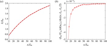
is plotted in figure 5(a). At
 $x=100L_{b}$
(the most distant streamwise location that we are considering in the present paper),
 ${\it\delta}\approx 1.92L_{b}$
. This means that the domain half-width is
 $L_{y}/2=L_{z}/2=7.5L_{b}\approx 3.9{\it\delta}$
at
 $x=100L_{b}$
. According to Redford et al. (Reference Redford, Castro and Coleman2012, p. 8), the critical value needed to ensure that the lateral boundary conditions do not affect the wake development is
 $L_{z}/2=L_{y}/2\approx 2.95{\it\delta}$
. The lateral dimensions of our domain therefore appear sufficiently large to avoid any significant contamination from the lateral boundaries even at
 $x=100L_{b}$
.
To further interrogate possible effects of wake confinement, the streamwise evolution of
 $\text{d}\langle u_{x}\rangle _{t}(x,L_{y},L_{z}/2)/\text{d}x$
(i.e. the
 $x$
derivative of the local streamwise velocity at the domain edge) is plotted in figure 5(b). It can be seen that the value of the
 $x$
derivative is very small and negative at all the streamwise locations considered in our study (
 ${\approx}-10^{-5}U_{\infty }/L_{b}$
). Secondly, close to the plate, the
 $x$
derivative is bigger because the velocity deficit is higher in agreement with mass conservation. At
 $x>40L_{b}$
, the value of the
 $x$
derivative is below approximately
 $-10^{-5}U_{\infty }/L_{b}$
and slowly tending to zero, as expected in the absence of confinement problems.
Streamwise evolution of the wake width
 ${\it\delta}/L_{b}$
(a) and of
 $(L_{b}/U_{\infty })\,\text{d}\langle u_{x}\rangle _{t}(x,L_{y},L_{z}/2)/\text{d}x$
(b).

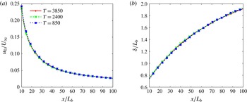
To assess the statistical convergence of the DNS data, statistics have been computed for three different averaging periods,
 $T=850L_{b}/U_{\infty }$
,
 $2400L_{b}/U_{\infty }$
and
 $3850L_{b}/U_{\infty }$
. The streamwise evolutions of the centreline velocity deficit and the wake width are plotted in figure 6 for the three cases. These mean quantities appear converged over the entire streamwise extent considered even for
 $T=850L_{b}/U_{\infty }$
. The same conclusion can be reached for the convergence of the centreline turbulent kinetic energy and dissipation. It must however be pointed out that
 $T=850L_{b}/U_{\infty }$
and even
 $T=2400L_{b}/U_{\infty }$
are not sufficient to converge the dissipation profiles at
 $x=90L_{b}$
and
 $x=100L_{b}$
even though
 $T=850L_{b}/U_{\infty }$
is sufficient at smaller values of
 $x/L_{b}$
.
Streamwise evolution of the centreline velocity deficit
 $u_{0}$
(a) and wake width
 ${\it\delta}$
(b) for three different averaging periods.

4. Experimental set-up
The experiments have been run in a low-turbulence wind tunnel with a measurement test section of
 $3~\text{ft}\times 3~\text{ft}$
(
 ${\sim}\!91~\text{cm}\times 91~\text{cm}$
) and length 4.25 m. The experimental set-up is based on the one used in Nedić et al. (Reference Nedić, Vassilicos and Ganapathisubramani2013b
). The plate has a reference length
 $L_{b}=64$
mm, with thickness 1.25 mm. The irregular plate is suspended in the centre of the wind tunnel normal to the laminar free stream using four 1 mm diameter piano wires. Free-stream velocity was kept fixed at
 $U_{\infty }=10$
m s
 $^{-1}$
. For that value, the velocity fluctuations around the mean are below 0.1 % when the test section is empty.
HWA measurements were taken downstream of the wake generator using a Dantec Dynamics 55P01 hot-wire probe, driven by a Dantec StreamLine CTA system. The Pt–W wires were
 $5~{\rm\mu}$
m in diameter, 3 mm long with a sensing length of 1.25 mm. The centreline of the wake was found by searching the maximum of the velocity deficit
 $u_{0}$
by successive iterations and with cross-wire checks (as described two paragraphs below). To obtain mean turbulent wake profiles, the probe was traversed at each one of the streamwise locations
 $x/L_{b}=10$
, 15, 20, 25, 30, 35, 40, 45 and 50 in 10 mm vertical intervals normal to the streamwise
 $x$
axis between
 $y=-250$
mm and
 $y=250$
mm. For each probe location, the acquisition time was
 $60$
s, with a sampling rate of
 $20$
kHz. Therefore, each profile acquisition took approximately 1 h of measurements. Two calibrations (one at the beginning and one at the end) were made for each profile, while temperature was monitored to not exceed a variation of
 $0.2\,^{\circ }$
C. The results reported here correspond to the lower half of the profiles measured, while the whole profile was used to check the positioning of the centre of the wake.
The axisymmetry of the flow was studied by taking radial–polar profiles at
 $x/L_{b}=10$
and
 $30$
. Measurements for these profiles were taken at eight different radial positions (5, 10, 20, 35, 50, 75, 100 and 150 cm) and 25 polar angles equispaced between
 $-{\rm\pi}$
and
 ${\rm\pi}$
with the same wire. Taking into account the centreline position, this gives 193 points at each streamwise position. Each point measurement has been acquired for
 $30$
s at 20 kHz and a new calibration has been taken each
 $30$
min with the same procedure as the one described in the previous paragraph for temperature variations.
Finally, a 55P51 X-wire probe (with same wires as that of our single-wire probe) was used for centreline measurements. At each centreline position, 30 min of data were acquired at 20 kHz. A new calibration was performed at every centreline position, and temperature variations were monitored as explained above. The X-wire measurements were used to calculate the centreline kinetic energy by assuming axisymmetry as
 $K_{0}=0.5(\langle u_{x}^{\prime 2}\rangle +2\langle u_{r}^{\prime 2}\rangle )^{1/2}$
, where
 $u_{x}^{\prime }$
and
 $u_{r}^{\prime }$
are, respectively, the streamwise and the radial fluctuating velocities.
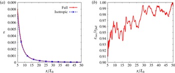
Centreline evolution of the full and isotropic dissipation (a) and of the ratio
 ${\it\varepsilon}_{iso}/{\it\varepsilon}_{full}$
(b). DNS data.

The turbulent energy dissipation was only estimated on the centreline from single-wire measurements acquired over
 $30$
min with 20 kHz sampling rate. It was calculated as
 ${\it\varepsilon}_{iso}=\int 15{\it\nu}k_{1}^{2}E_{11}\,\text{d}k_{1}$
, where
 $E_{11}(k_{1})$
is the one-dimensional power spectrum and
 $k_{1}=2{\rm\pi}f/U$
, where
 $f$
is a Fourier frequency in hertz. We therefore assume local isotropy at the centreline and we use the Taylor hypothesis (the turbulence intensity based on the local mean flow velocity is always below, and in most cases much smaller than, 12 %). The validity of the local isotropy assumption was checked with our DNS data, and in figure 7 we compare
 ${\it\varepsilon}_{iso}=15{\it\nu}\langle (\partial u_{x}^{\prime }/\partial x)^{2}\rangle$
with the actual dissipation rate
 ${\it\varepsilon}_{full}=2{\it\nu}\langle s_{ij}s_{ij}\rangle$
, where
 $s_{ij}=(\partial u_{i}^{\prime }/\partial x_{j}+\partial u_{j}^{\prime }/\partial x_{i})/2$
. It is clear from figure 7(b) that
 ${\it\varepsilon}_{iso}/{\it\varepsilon}_{full}$
lies between 0.94 and 1 in the range
 $10\leqslant x/L_{b}\leqslant 50$
and that it quickly tends to 1 as
 $x/L_{b}$
increases.
The acquisition time of the centreline single-wire measurements being
 $30$
min, of the order of 100 000 integral time scales at each streamwise position were recorded, thereby allowing good large-scale resolution. The Kolmogorov frequency was always smaller than half our sampling frequency (which is 20 kHz) except at the position closest to the plate (
 $x/L_{b}=10$
), where it was 12 kHz. At this position, where our Kolmogorov microscale
 ${\it\eta}$
is at its smallest,
 ${\it\eta}=140~{\rm\mu}$
m, but it grows with streamwise distance to reach
 ${\it\eta}\approx 0.4$
mm at
 $x/L_{b}=50$
. We checked that the main contribution to the integral
 $\int 15{\it\nu}k_{1}^{2}E_{11}\,\text{d}k_{1}$
comes in all our cases from wavenumbers
 $k_{1}{\it\eta}\leqslant 0.5$
and that variations of the dissipation spectrum at wavenumbers higher than
 $k_{1}{\it\eta}=0.5$
modelled by various exponential shapes imply variations in our estimates of
 ${\it\varepsilon}_{iso}$
of less than 6 %.
5. Reynolds-averaged momentum equation balance
The analysis that leads to the streamwise scalings of the velocity deficit and width of turbulent wakes is usually carried out on the boundary layer approximation of the Reynolds-averaged momentum balance (see Townsend Reference Townsend1976; Pope Reference Pope2000). In this section we use our DNS to check and confirm the leading and neglected terms in this balance equation.
In Cartesian coordinates, the full Reynolds-averaged streamwise momentum equation is given by
 $$\begin{eqnarray}\displaystyle & & \displaystyle \frac{\partial U}{\partial t}+U\frac{\partial U}{\partial x}+\langle u_{y}\rangle \frac{\partial U}{\partial y}+\langle u_{z}\rangle \frac{\partial U}{\partial z}\nonumber\\ \displaystyle & & \displaystyle \quad =-\frac{1}{{\it\rho}}\frac{\partial \langle p\rangle }{\partial x}-\frac{\partial \langle u_{x}^{\prime }u_{x}^{\prime }\rangle }{\partial x}-\frac{\partial \langle u_{x}^{\prime }u_{y}^{\prime }\rangle }{\partial y}-\frac{\partial \langle u_{x}^{\prime }u_{z}^{\prime }\rangle }{\partial z}+{\it\nu}\left(\frac{\partial ^{2}U}{\partial x^{2}}+\frac{\partial ^{2}U}{\partial y^{2}}+\frac{\partial ^{2}U}{\partial z^{2}}\right),\end{eqnarray}$$
where
 $u_{x}^{\prime }$
,
 $u_{y}^{\prime }$
and
 $u_{z}^{\prime }$
are the fluctuating velocity components in the
 $x$
,
 $y$
and
 $z$
directions, respectively.
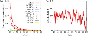
For sufficiently converged statistics, the first term on the left-hand side vanishes, i.e.
 $\partial U/\partial t\approx 0$
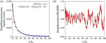
. The centreline evolution of all the other terms is plotted in figure 8(a) and the ratio between the left-hand side (LHS) and the right-hand side (RHS) of (5.1) is plotted in figure 8(b). It can be seen in figure 8(b) that the full momentum balance equation (5.1) is represented accurately enough by our calculations on the centreline (the error made in the mean momentum equation budget is almost everywhere below 6 %, except at the very end of the domain, where it is 10 %). It can also be seen in figure 8(a) that the three terms
 $U\,\partial U/\partial x$
,
 $-\partial \langle u_{x}^{\prime }u_{y}^{\prime }\rangle /\partial y$
and
 $-\partial \langle u_{x}^{\prime }u_{z}^{\prime }\rangle /\partial z$
are the main contributors to this momentum balance. We have checked that all the other terms are at least two orders of magnitude smaller than these three terms, so that we can use the following simplified equation:
 $$\begin{eqnarray}U\frac{\partial U}{\partial x}=-\frac{\partial \langle u_{x}^{\prime }u_{y}^{\prime }\rangle }{\partial y}-\frac{\partial \langle u_{x}^{\prime }u_{z}^{\prime }\rangle }{\partial z}.\end{eqnarray}$$
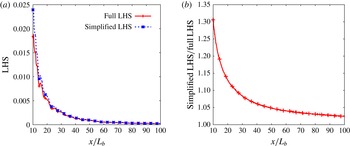
This is indeed the simplified form of the mean momentum equation, which is typically used to study turbulent wakes. The centreline evolutions of the LHS and RHS of the simplified balance equation (5.2) are plotted in figure 9(a) and their ratio is plotted in figure 9(b). This figure confirms that the simplified Reynolds-averaged momentum equation (5.2) is valid in our turbulent wake where
 $\text{LHS}\approx \text{RHS}$
for all streamwise locations within 8 %. The viscous term, in particular, is always at least two orders of magnitude smaller than these three main terms. We stress this point because it means that the low-Reynolds-number scalings (1.3) and (1.4) (see Johansson et al.
Reference Johansson, George and Gourlay2003, for details) cannot be expected in our data.
Centreline evolution of each term involved in the full Reynolds-averaged momentum equation (5.1) (a) and of the ratio LHS/RHS (b). DNS data.

Centreline evolution of the LHS and RHS of the simplified Reynolds-averaged equation for the axisymmetric wake (5.2) (a) and of the ratio LHS/RHS (b). DNS data.

To derive scalings for the axisymmetric wake, it is also usual to consider the first-order approximation of (5.2), which is
 $$\begin{eqnarray}U_{\infty }\frac{\partial }{\partial x}(U_{\infty }-U)=\frac{\partial \langle u_{x}^{\prime }u_{y}^{\prime }\rangle }{\partial y}+\frac{\partial \langle u_{x}^{\prime }u_{z}^{\prime }\rangle }{\partial z}\end{eqnarray}$$
in terms of the mean velocity deficit
 $U_{\infty }-U$
. The centreline evolution of the full LHS of (5.2) is plotted together with its first-order counterpart of (5.3) in figure 10. A good agreement is found between the two relations, with an error that is quickly decreasing and that is always below 10 % for
 $x\geqslant 20L_{b}$
.


6. Axisymmetry of wake statistics
The second step of this analysis is to ascertain the statistical axisymmetry of the wakes generated by our irregular plate. Our DNS provides three-dimensional fields in the entire computational domain, and we use them to check polar variations of the mean velocity
 $U$
, the Reynolds shear stress
 $R_{xr}\equiv \langle u_{x}^{\prime }u_{r}^{\prime }\rangle$
, the turbulent kinetic energy
 $K$
and the dissipation rate
 ${\it\varepsilon}$
. Our HWA measurements provide us with streamwise mean velocities and streamwise Reynolds stresses
 $R_{xx}\equiv \langle u_{x}^{\prime }u_{x}^{\prime }\rangle$
in cross-sections of the wake at
 $x=10L_{b}$
and
 $x=30L_{b}$
. We use our HWA data in conjunction with our DNS data to check both axisymmetry and agreement between data.
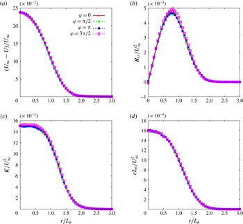
Normalised velocity deficit (a), Reynolds shear stress (b), turbulent kinetic energy (c) and dissipation rate of turbulent kinetic energy (d) profiles from the DNS case at the downstream location
 $x/L_{b}=10$
for four different polar angles
 ${\it\varphi}$
.

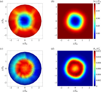
Maps of the mean streamwise velocity
 $U/U_{\infty }$
for the HWA case (a) and for the DNS case (b), with the same colour coding, and of the mean streamwise Reynolds stress
 $R_{xx}/U_{\infty }^{2}$
for the HWA (c) and the DNS (d), again with the same colour coding. All these maps are taken at
 $x=10L_{b}$
.

In figure 11 we plot streamwise mean velocity, Reynolds stress, turbulent kinetic energy and dissipation radial profiles at four different polar angles
 ${\it\varphi}$
, all obtained from our DNS at
 $x/L_{b}=10$
. These wake statistics are already quite axisymmetric at this near-field location
 $x=10L_{b}$
. As shown in figure 12(a,c), this observation is confirmed for the mean flow statistics and
 $R_{xx}$
by our HWA measurements at the same location. Figure 12 also shows satisfactory agreement between the numerical simulation and the experiments.
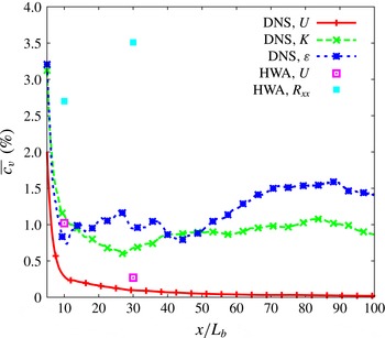
A more quantitative evaluation of the flow’s statistical axisymmetry can be obtained by computing the mean values of the coefficient of variance,
 $$\begin{eqnarray}c_{v}(x,r)\equiv 100\frac{\sqrt{(1/N_{{\it\varphi}})\displaystyle \mathop{\sum }_{{\it\varphi}}(S(x,r,{\it\varphi})-\langle S\rangle (x,r))^{2}}}{\langle S\rangle (x,r)},\end{eqnarray}$$
where
 $N_{{\it\varphi}}$
is the number of polar angles and
 $S$
stands for mean flow, kinetic energy or dissipation rate of turbulent kinetic energy. The streamwise variations of the radially averaged coefficient of variance
 $\overline{c_{v}}(x)\equiv (1/N_{r})\sum _{r}c_{v}(x,r)$
are plotted in figure 13 for the DNS and HWA cases (only at
 $x=10L_{b}$
and
 $x=30L_{b}$
). It must be mentioned here that the coefficient of variance has not been computed for the Reynolds shear stress component
 $R_{xr}$
because of the small values it takes close to the centreline leading to artificially high values of
 $c_{v}$
. Because the same problem can appear at large radii where
 $K$
and
 ${\it\varepsilon}$
tend to zero, the radially averaged coefficients of variance are computed for
 $r\in [0;L_{b}]$
. Figure 13 shows that, at
 $x=10L_{b}$
, there is already less than 4 % variation in all statistics. Hence, both our DNS calculations and our HWA measurements demonstrate the good axisymmetry of the flow at
 $x>10L_{b}$
.
Streamwise evolution of the radially averaged coefficient of variance
 $\overline{c_{v}}$
for the mean velocity, turbulent kinetic energy and the dissipation profiles of the DNS case and for the mean velocity and streamwise Reynolds stress of the HWA case at
 $x=10L_{b}$
and
 $x=30L_{b}$
.

7. Similarity of the axisymmetric turbulent wake
The axisymmetry of the wake having now been demonstrated for both the DNS and the HWA cases, the next step is to investigate the similarity properties of the mean flow statistics. The study of the dissipation law and its consequences on the velocity deficit and wake width scalings follows naturally in the next section. In this section we use our DNS and HWA to analyse the streamwise self-similarity of the mean velocity, Reynolds stress, turbulent kinetic energy and dissipation profiles. Comparisons between our DNS and our HWA data are made for the mean velocity and streamwise Reynolds stress profiles.
The following self-similar forms are considered for the mean velocity, Reynolds stresses, turbulent kinetic energy and dissipation profiles:
 $$\begin{eqnarray}\displaystyle U_{\infty }-U(x,r) & = & \displaystyle u_{0}(x)f({\it\eta}),\end{eqnarray}$$
 $$\begin{eqnarray}\displaystyle R_{xx}(x,r) & = & \displaystyle G_{01}(x)g_{11}({\it\eta}),\end{eqnarray}$$
 $$\begin{eqnarray}\displaystyle R_{rr}(x,r) & = & \displaystyle G_{02}(x)g_{22}({\it\eta}),\end{eqnarray}$$
 $$\begin{eqnarray}\displaystyle R_{{\it\varphi}{\it\varphi}}(x,r) & = & \displaystyle G_{03}(x)g_{33}({\it\eta}),\end{eqnarray}$$
 $$\begin{eqnarray}\displaystyle R_{xr}(x,r) & = & \displaystyle R_{0}(x)g_{12}({\it\eta}),\end{eqnarray}$$
 $$\begin{eqnarray}\displaystyle K(x,r) & = & \displaystyle K_{0}(x)h({\it\eta}),\end{eqnarray}$$
 $$\begin{eqnarray}\displaystyle {\it\varepsilon}(x,r) & = & \displaystyle D_{0}(x)e({\it\eta}),\end{eqnarray}$$
 ${\it\eta}=r/{\it\delta}$
and
 $f(0)=1$
.
We first investigate whether the profiles (7.1)–(7.7) are self-similar, as this is a basic property that must be addressed before embarking on the second question, which concerns the actual scalings of the
 $x$
-dependent prefactors
 $u_{0}(x)$
,
 $G_{0i}(x)$
(
 $i=1,2,3$
),
 $R_{0}(x)$
,
 $K_{0}(x)$
and
 $D_{0}(x)$
. If a profile is self-similar, then it must be self-similar with the
 $x$
-dependent prefactor being the profile’s maximum value along
 $r$
. We can therefore test for self-similarity just by taking
 $G_{0i}(x)=\max _{r}(R_{ii})$
,
 $R_{0}(x)=\max _{r}(R_{xr})$
,
 $K_{0}(x)=\max _{r}(K)$
and
 $D_{0}(x)=\max _{r}({\it\epsilon})$
. The prefactor
 $u_{0}(x)$
is a special case as it is the maximum value of
 $U_{\infty }-U(x,r)$
anyway, given that
 $f({\it\eta})\leqslant f(0)=1$
.
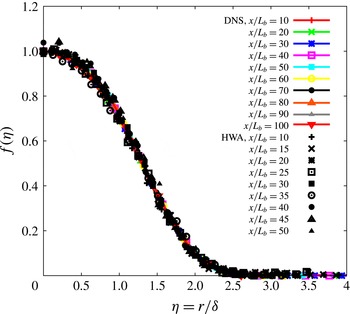
Streamwise mean velocity profiles are plotted in figure 14 for different streamwise distances using the similarity scaling defined in (7.1). These profiles are clearly self-similar for
 $x\geqslant 10L_{b}$
, with very good agreement between the DNS and the HWA results. The DNS data show that the self-similarity of the mean profiles is maintained in the range
 $x\in [50L_{b};100L_{b}]$
where HWA measurements are missing given that the wind tunnel test section is half as long as the DNS domain.
Mean flow profiles at different streamwise distances plotted using similarity scaling for both the DNS and the HWA cases.

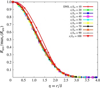
The streamwise, radial and polar Reynolds stress profiles
 $R_{xx}(x,r)$
,
 $R_{rr}(x,r)$
and
 $R_{{\it\varphi}{\it\varphi}}(x,r)$
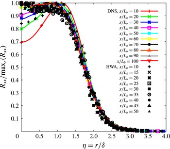
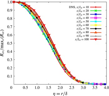
are plotted in figures 15–17. These are normal Reynolds stresses, which do not feature in the similarity theory of George (Reference George, George and Arndt1989) even though the first two do feature in the similarity theory of Townsend (Reference Townsend1976). Note the satisfactory agreement between our HWA and our DNS streamwise Reynolds stress profiles (figure 15). Differences between HWA and DNS data can however be noted for
 $x/L_{b}<40$
and
 ${\it\eta}<1$
. These differences could be due to different Reynolds number values in the experiment and the simulation. Our data do not suggest that these Reynolds stresses are self-similar except for the polar one,
 $R_{{\it\varphi}{\it\varphi}}(x,r)$
, which does appear self-similar for
 $x/L_{b}\geqslant 20$
. (The streamwise Reynolds stress profiles obtained in the wind tunnel may, arguably, be self-similar for, approximately,
 $x\geqslant 30L_{b}$
while the equivalent DNS profiles may perhaps be close to self-similar at
 $x\geqslant 50L_{b}$
.)
Streamwise Reynolds stress profiles at different streamwise distances plotted using similarity scaling with
 $G_{01}=\max _{r}(R_{xx})$
for both the DNS and the HWA cases.

Radial Reynolds stress profiles at different streamwise distances plotted using similarity scaling with
 $G_{02}=\max _{r}(R_{rr})$
for the DNS case.

Polar Reynolds stress profiles at different streamwise distances plotted using similarity scaling with
 $G_{03}=\max _{r}(R_{{\it\varphi}{\it\varphi}})$
for the DNS case.

The similarity theories of Townsend (Reference Townsend1976) and George (Reference George, George and Arndt1989) are both based on the average momentum and turbulent kinetic energy equations. George (Reference George, George and Arndt1989) used the momentum balance (5.3), which, in cylindrical coordinates
 $(x,r,{\it\varphi})$
, becomes
 $$\begin{eqnarray}U_{\infty }\frac{\partial }{\partial x}(U_{\infty }-U)=\frac{1}{r}\frac{\partial r\langle u_{x}^{\prime }u_{r}^{\prime }\rangle }{\partial r},\end{eqnarray}$$
and the turbulent kinetic energy evolution equation
 $$\begin{eqnarray}U_{\infty }\frac{\partial }{\partial x}K=-\langle u_{x}^{\prime }u_{r}^{\prime }\rangle \frac{\partial U}{\partial r}+T-{\it\epsilon},\end{eqnarray}$$
where
 $T$
and
 ${\it\epsilon}$
are, respectively, the transport term and the turbulence dissipation rate, and where the production term is approximated by
 $-\langle u_{x}^{\prime }u_{r}^{\prime }\rangle \,\partial U/\partial r$
. His theory therefore relies on this production term approximation and on the self-similarity of the
 $U_{\infty }-U$
,
 $\langle u_{x}^{\prime }u_{r}^{\prime }\rangle$
,
 $K$
,
 ${\it\epsilon}$
and transport term profiles. Our DNS provides access to all these quantities except the transport term
 $T\equiv \partial (\langle u_{j}^{\prime }p^{\prime }/{\it\rho}\rangle +{\textstyle \frac{1}{2}}\langle u_{i}^{\prime 2}u_{j}^{\prime }\rangle -2{\it\nu}\langle u_{i}^{\prime }s_{ij}\rangle )/\partial x_{j}$
, which involves spatial derivatives of third-order fluctuating velocity statistics and is therefore very expensive to compute because of the large computational time required to obtain converged statistics. (The average momentum and turbulent kinetic energy equations used by Townsend (Reference Townsend1976) have a couple more terms, which involve the streamwise and radial Reynolds stresses; Townsend (Reference Townsend1976) assumed these stresses to be self-similar too.)
The self-similarity of the mean flow profile has already been established. We therefore now consider the self-similarity of the Reynolds shear stress
 $\langle u_{x}^{\prime }u_{r}^{\prime }\rangle$
, the turbulent kinetic energy
 $K$
and the dissipation rate
 ${\it\epsilon}$
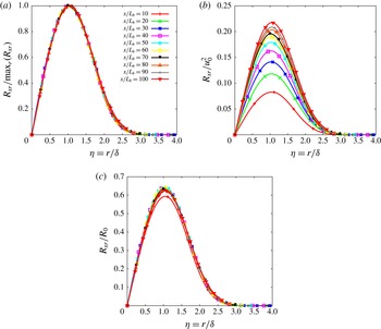
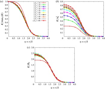
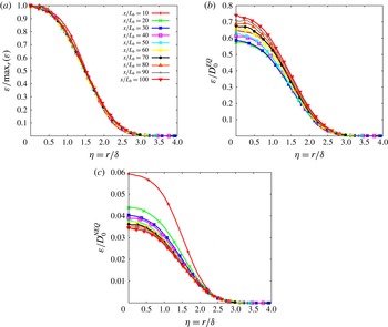
. We plot these profiles in figures 18(a), 19(a) and 20(a) with
 $R_{0}$
,
 $K_{0}$
and
 $D_{0}$
set to be the maximum values along
 $r$
of
 $\langle u_{x}^{\prime }u_{r}^{\prime }\rangle (x,r)$
,
 $K(x,r)$
and
 ${\it\epsilon}(x,r)$
, i.e.
 $R_{0}(x)=\max _{r}(R_{xr})$
,
 $K_{0}(x)=\max _{r}(K)$
and
 $D_{0}(x)=\max _{r}({\it\epsilon})$
. These three figure panels rather strongly suggest that these three profiles are all self-similar, in the region
 $x/L_{b}\geqslant 10$
for
 $\langle u_{x}^{\prime }u_{r}^{\prime }\rangle (x,r)$
and
 ${\it\epsilon}(x,r)$
and in the region
 $x/L_{b}\geqslant 20$
for
 $K(x,r)$
.
Reynolds shear stress profiles at different streamwise distances plotted using similarity scalings with
 $R_{0}=\max _{r}(R_{xr})$
(a),
 $R_{0}\sim u_{0}^{2}$
(b) and
 $R_{0}\sim u_{0}U_{\infty }(\text{d}{\it\delta}/\text{d}x)$
(c) for the DNS case.

The self-similarity of
 $U_{\infty }-U$
and
 $\langle u_{x}^{\prime }u_{r}^{\prime }\rangle$
in the region
 $x/L_{b}\geqslant 10$
and the validity of the mean momentum equation in the simplified approximate form (7.8) directly imply, as is well known (see George Reference George, George and Arndt1989), that
 $u_{0}{\it\delta}^{2}=U_{\infty }{\it\theta}^{2}$
and
 $R_{0}=U_{\infty }u_{0}\,\text{d}{\it\delta}/\text{d}x$
. Figure 18(c) shows that our DNS supports the prediction
 $R_{0}=U_{\infty }u_{0}(\text{d}/\text{d}x){\it\delta}$
, at least in the region
 $x/L_{b}\geqslant 20$
. Incidentally, figure 18(b) shows that the assumption
 $R_{0}\sim u_{0}^{2}$
made by Tennekes & Lumley (Reference Tennekes and Lumley1972) to avoid using the energy equation (7.9) is not supported by our DNS.
The energy equation (7.9) and the self-similarities of
 $K$
,
 $U_{\infty }-U$
,
 $\langle u_{x}^{\prime }u_{r}^{\prime }\rangle$
and
 ${\it\epsilon}$
in the region
 $x/L_{b}\geqslant 20$
imply, as is also well known (see George Reference George, George and Arndt1989), that
 $K_{0}\sim u_{0}^{2}$
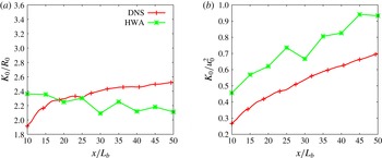
(the analysis of Townsend (Reference Townsend1976) also led to this relation, but with more constraining, albeit similar, assumptions). However, our DNS does not endorse this scaling, as can be seen in figure 19(b). In fact, figure 19 shows that
 $K_{0}$
scales in the same way as
 $R_{0}$
in the region
 $x/L_{b}\geqslant 20$
, i.e.
 $$\begin{eqnarray}K_{0}\sim U_{\infty }u_{0}\frac{\text{d}{\it\delta}}{\text{d}x}.\end{eqnarray}$$
This is a relation that our higher-Reynolds-number HWA measurements strongly endorse in the region
 $10\leqslant x/L_{b}\leqslant 50$
where HWA measurements were taken; see figure 21, where centreline HWA and DNS data are plotted together. The scaling (7.10) was also observed in the HWA measurements of Nedic (Reference Nedic2013).
Turbulent kinetic energy profiles at different streamwise distances plotted using similarity scaling with
 $K_{0}=\max _{r}(K)$
(a),
 $K_{0}\sim u_{0}^{2}$
(b) and
 $K_{0}\sim R_{0}\sim u_{0}U_{\infty }(\text{d}{\it\delta}/\text{d}x)$
(c) for the DNS case.

The failure of
 $K_{0}\sim u_{0}^{2}$
points to a failure of (7.9) because the approximation
 $-\langle u_{x}^{\prime }u_{r}^{\prime }\rangle (\partial U/\partial r)$
for the production term is essential in obtaining
 $K_{0}\sim u_{0}^{2}$
. In fact, one cannot expect the production term to equal
 $-\langle u_{x}^{\prime }u_{r}^{\prime }\rangle (\partial U/\partial r)$
on the centreline where
 $-\langle u_{x}^{\prime }u_{r}^{\prime }\rangle =0$
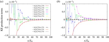
. Indeed, as shown in figure 22, our DNS shows that the production term
 $P$
is dominated by normal stress terms on the centreline and that these normal stress terms are not negligible at
 $r/L_{b}=0.5$
either, in particular
 $\langle u_{x}^{\prime }u_{x}^{\prime }\rangle (\partial U/\partial x)$
, which is comparable in magnitude to
 $-\langle u_{x}^{\prime }u_{r}^{\prime }\rangle (\partial U/\partial r)$
. We must therefore replace (7.9) by
 $$\begin{eqnarray}U_{\infty }\frac{\partial K}{\partial x}=P+T-{\it\epsilon},\end{eqnarray}$$
and we must not use a self-similarity ansatz for
 $P$
since, as we have seen, the normal Reynolds stresses
 $R_{xx}$
,
 $R_{rr}$
and
 $R_{{\it\varphi}{\it\varphi}}$
are not quite self-similar. Nevertheless, the self-similarities of
 $K$
and
 ${\it\epsilon}$
imply that
 $P+T$
must be self-similar.
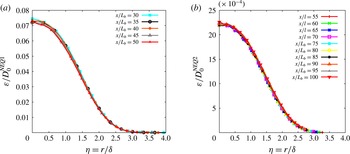
Dissipation profiles at different streamwise distances plotted using similarity scaling with
 $D_{0}=\max _{r}({\it\varepsilon})$
(a),
 $D_{0}=D_{0}^{EQ}=K_{0}^{3/2}/{\it\delta}$
(b) and
 $D_{0}=D_{0}^{NEQ1}=(U_{\infty }l/{\it\nu})(u_{0}{\it\delta}/{\it\nu})^{-1}K_{0}^{3/2}/{\it\delta}$
(c) for the DNS case.

Centreline evolution of the ratio
 $K_{0}/R_{0}$
(a) and
 $K_{0}/u_{0}^{2}$
(b) for both the DNS and the HWA cases.

Streamwise evolution of each contribution to the turbulent kinetic energy production term for the DNS data on the centreline (a) and at
 $y/Lb=0.5$
and
 $z/L_{b}=0$
off the centreline (b).

Injection of the self-similar forms
 $K(x,r)=K_{0}h({\it\eta})$
and
 ${\it\epsilon}(x,r)=D_{0}e({\it\eta})$
in (7.11) yields
 $$\begin{eqnarray}U_{\infty }\frac{\text{d}K_{0}}{\text{d}x}\sim \frac{U_{\infty }K_{0}}{{\it\delta}}\frac{\text{d}{\it\delta}}{\text{d}x}\sim D_{0}.\end{eqnarray}$$
Following Nedić et al. (Reference Nedić, Vassilicos and Ganapathisubramani2013b ) we use
 $$\begin{eqnarray}D_{0}\sim \left(\frac{U_{\infty }L_{b}}{{\it\nu}}\right)^{m}\left(\frac{\sqrt{K_{0}}{\it\delta}}{{\it\nu}}\right)^{-m}\frac{K_{0}^{3/2}}{{\it\delta}},\end{eqnarray}$$
corresponding to the non-equilibrium dissipation law (1.7), (2.3) and (2.4) with
 $n=m$
. We limit ourselves to
 $n=m$
, as this is enough for the purposes of this present paper, but it is straightforward also to consider the more general case where the exponents
 $n$
and
 $m$
are not necessarily equal.
In the case where
 $m=1$
, which is also the case reported in the literature at high enough Reynolds numbers (see Goto & Vassilicos Reference Goto and Vassilicos2015; Vassilicos Reference Vassilicos2015),
 $D_{0}\sim (U_{\infty }L_{b}/{\it\nu})(\sqrt{K_{0}}{\it\delta}/{\it\nu})^{-1}K_{0}^{3/2}/{\it\delta}$
(equation (7.13) with
 $m=1$
) and
 $(U_{\infty }K_{0}/{\it\delta})\,\text{d}{\it\delta}/\text{d}x\sim D_{0}$
(equation (7.12)) lead immediately to (1.9), which, in turn, leads to (1.8) if use is made of
 $u_{0}{\it\delta}^{2}=U_{\infty }{\it\theta}^{2}$
. These high-Reynolds-number scalings of
 ${\it\delta}(x)$
and
 $u_{0}(x)$
have already been observed in the turbulent wake experiments of Nedić et al. (Reference Nedić, Vassilicos and Ganapathisubramani2013b
).
However, the centreline dissipation rate
 $D_{0}$
does not scale as
 $D_{0}^{NEQ1}=(U_{\infty }L_{b}/{\it\nu})\times (\sqrt{K_{0}}{\it\delta}/{\it\nu})^{-1}K_{0}^{3/2}/{\it\delta}$
in the range
 $10\leqslant x/L_{b}\leqslant 100$
, but it does not scale as
 $D_{0}^{EQ}=K_{0}^{3/2}/{\it\delta}$
either in that range (see figure 20). These DNS results suggest that, when considering the full streamwise range
 $x\in [10L_{b};100L_{b}]$
, neither the equilibrium dissipation law nor the non-equilibrium dissipation law (at least with
 $n=m=1$
) are recovered in the axisymmetric turbulent wake generated by our irregular plate. To understand better how the dissipation is evolving in our turbulent axisymmetric wakes, the streamwise evolution of the dissipation is analysed in more detail in the next section.
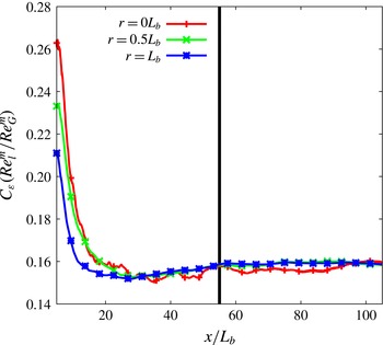
Streamwise variation of the dissipation constant
 $C_{{\it\varepsilon}}$
(a) and
 $C_{{\it\varepsilon}}\times (\mathit{Re}_{l}/\mathit{Re}_{G})$
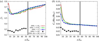
(b) for both the DNS and HWA cases. The black vertical line corresponds to
 $x=55L_{b}$
.

8. Streamwise evolution of the centreline dissipation
Defining
 $C_{{\it\epsilon}}$
by
 $$\begin{eqnarray}{\it\varepsilon}=C_{{\it\varepsilon}}K^{3/2}/{\it\delta}\end{eqnarray}$$
and evaluating it on the centreline
 $r=0$
as a function of streamwise distance
 $x$
generates figure 23, where we plot data obtained by HWA and DNS. The first obvious qualitative observation is that the centreline
 $C_{{\it\epsilon}}$
grows with streamwise distance
 $x$
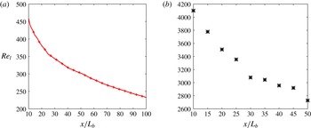
even though the local Reynolds number decreases with
 $x$
(see figure 24), in clear disagreement with the equilibrium law
 $C_{{\it\epsilon}}=\text{const}$
. Both the DNS and the HWA data exhibit this behaviour. In fact, off-centreline DNS data also plotted in figure 23 show that this behaviour is not specific to the centreline. It is also observed along streamwise
 $r=L_{b}/2$
and
 $r=L_{b}$
lines. To check if this growth with
 $x$
can be represented by the non-equilibrium dissipation law (1.7) one needs to check if it is matched by the growth of
 $(\mathit{Re}_{G}^{m}/\mathit{Re}_{l}^{n})$
in the
 $x$
direction. We therefore add a plot of
 $(\mathit{Re}_{l}^{n}/\mathit{Re}_{G}^{m})\times C_{{\it\varepsilon}}$
for
 $n=m=1$
in figure 23. The HWA data show good agreement with
 $C_{{\it\varepsilon}}\sim (\mathit{Re}_{G}/\mathit{Re}_{l})$
in the range
 $15\leqslant x/L_{b}\leqslant 50$
and the DNS data are clearly closer to
 $C_{{\it\varepsilon}}\sim (\mathit{Re}_{G}/\mathit{Re}_{l})$
than to
 $C_{{\it\epsilon}}=\text{const.}$
in that range. The better defined
 $C_{{\it\varepsilon}}\sim (\mathit{Re}_{G}/\mathit{Re}_{l})$
scaling in the higher-Reynolds-number HWA data than in the lower-Reynolds-number DNS data agrees with the observations of Goto & Vassilicos (Reference Goto and Vassilicos2015), who found that the local Taylor length-scale-based Reynolds number
 $\mathit{Re}_{{\it\lambda}}$
needs to be higher than 100 for
 $(\mathit{Re}_{l}/\mathit{Re}_{G})\times C_{{\it\varepsilon}}$
to be a sufficiently well-defined constant. Indeed,
 $\mathit{Re}_{{\it\lambda}}$
is below
 $100$
in the DNS region
 $15\leqslant x/L_{b}\leqslant 50$
, and again in agreement with Goto & Vassilicos (Reference Goto and Vassilicos2015),
 $(\mathit{Re}_{l}/\mathit{Re}_{G})\times C_{{\it\varepsilon}}$
is larger for our DNS than for our HWA data, which are characterised by
 $\mathit{Re}_{{\it\lambda}}$
values between 200 and 300.
A close look at the DNS data in figure 23 may suggest a slope change at
 $x/L_{b}\approx 55$
. Downstream of
 $x\approx 55L_{b}$
(where
 $\mathit{Re}_{{\it\lambda}}$
is below 60), the product
 $(\mathit{Re}_{l}/\mathit{Re}_{G})\times C_{{\it\varepsilon}}$
appears to be quite clearly slightly decreasing, palpably more than in the region
 $15\leqslant x/L_{b}\leqslant 50$
, where it might be closer to a constant. While our DNS and HWA observations support the non-equilibrium dissipation law (1.7) with
 $n=m\approx 1$
in the region
 $x\in [15L_{b};50L_{b}]$
, the DNS data suggest a change in the exponents
 $m$
and
 $n$
further downstream. We elaborate on this point in the next section.
Streamwise variation of the local Reynolds number
 $\mathit{Re}_{l}=\sqrt{K_{0}}{\it\delta}/{\it\nu}$
: (a) for the DNS and (b) for the HWA.

9. Wake width and velocity deficit scalings
The theoretical arguments developed at the end of § 7 for the prediction of the wake width and the centreline velocity deficit rely on the axisymmetry and self-similarity of
 $U_{\infty }-U$
,
 $\langle u_{x}^{\prime }u_{r}^{\prime }\rangle$
,
 $K$
and
 ${\it\epsilon}$
and the use of the streamwise average momentum and turbulent kinetic energy equations (7.8) and (7.11). All these have been reasonably well verified by our DNS and our HWA measurements in the region between approximately
 $10L_{b}$
and
 $100L_{b}$
. However, our prediction method also relies on the dissipation scaling, and the previous section suggests two different scalings in two different regions, one for
 $x\in [15L_{b};50L_{b}]$
and one for
 $x\in \, ]55L_{b};100L_{b} ]$
(only accessible with our DNS). Since our prediction method has been developed only for the dissipation scaling (7.13) with
 $m=1$
, i.e.
 $C_{{\it\varepsilon}}\sim (\mathit{Re}_{G}/\mathit{Re}_{l})$
, we now need to extend it to any value of
 $m$
, i.e. to the non-equilibrium dissipation law (1.7), (2.3) and (2.4) for any value of
 $n=m$
. Generalisation to
 $n\not =m$
is straightforward but not necessary in this work.
As already explained in § 7, our revised and modified George theory for
 $m=1$
proceeds as follows. Self-similarity of (7.11) yields
 $D_{0}\sim (U_{\infty }K_{0}/{\it\delta})\,\text{d}{\it\delta}/\text{d}x$
and use of (7.13) can only provide a closed set of equations when
 $m=1$
, in which case it leads to (1.9). In turn, the integral form
 $u_{0}{\it\delta}^{2}=U_{\infty }{\it\theta}^{2}$
of (7.8) yields (1.8).
When
 $m\not =1$
an additional relation is needed and we obtain it on the basis of an assumption of constant anisotropy. According to this assumption, the correlation function between the fluctuating velocity components
 $u_{x}^{\prime }$
and
 $u_{r}^{\prime }$
and the ratios of the root-mean-square (r.m.s.) values of
 $u_{x}^{\prime }$
,
 $u_{r}^{\prime }$
and
 $u_{{\it\varphi}}^{\prime }$
are constant on
 $r={\it\delta}(x)$
, the surface defining the locations of the maximum Reynolds shear stress, over the region considered, i.e.
 $x\in [15L_{b};100L_{b}]$
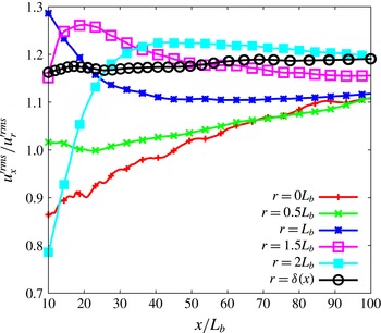
in our case. This assumption and the precise region where it holds will need to be investigated and explained in future studies. Here we note that our DNS data support it (see figure 25) and that it is capable to close our problem for any value of
 $m$
and return predictions for the wake width and the centreline velocity deficit that agree with numerical calculations and experimental measurements.
Ratios of the r.m.s. of
 $u_{x}^{\prime }$
to the r.m.s. of
 $u_{r}^{\prime }$
as functions of
 $x/L_{b}$
along the centreline (
 $r=0$
) and on various axisymmetric surfaces
 $r=L_{b}/2$
,
 $L_{b}$
,
 $3L_{b}/2$
,
 $2L_{b}$
and
 ${\it\delta}(x)$
for the DNS data. Note how the most constant value of this ratio is found on the surface
 $r={\it\delta}(x)$
.

The assumption of constant anisotropy implies that the turbulent kinetic energy is proportional to the Reynolds shear stress on the surface
 $r={\it\delta}(x)$
, i.e.
 $K_{0}\sim R_{0}$
. Given that self-similarity of (7.9) implies
 $R_{0}\sim U_{\infty }u_{0}(\text{d}{\it\delta}/\text{d}x)$
, it then follows that
 $K_{0}\sim U_{\infty }u_{0}(\text{d}{\it\delta}/\text{d}x)$
, i.e. (7.10) which is supported by both our DNS and our HWA measurements. Combining (7.10) with
 $D_{0}\sim (U_{\infty }K_{0}/{\it\delta})\,\text{d}{\it\delta}/\text{d}x$
(from the similarity of the turbulent kinetic energy equation) and (7.13) leads to
 $$\begin{eqnarray}\frac{{\it\delta}(x)}{{\it\theta}}=B\left(\frac{x-x_{0}}{{\it\theta}}\right)^{{\it\beta}},\end{eqnarray}$$
where
 ${\it\beta}=(1+m)/(3+m)$
and
 $B\sim (L_{b}/{\it\theta})^{2m/(3+m)}$
. With
 $u_{0}{\it\delta}^{2}=U_{\infty }{\it\theta}^{2}$
this relation implies
 $$\begin{eqnarray}\frac{u_{0}(x)}{U_{\infty }}=A\left(\frac{x-x_{0}}{{\it\theta}}\right)^{{\it\alpha}},\end{eqnarray}$$
where
 ${\it\alpha}=-2{\it\beta}=-2(1+m)/(3+m)$
and
 $A=B^{-2}$
. Note that
 $m=0$
yields the well-known equilibrium scalings
 ${\it\delta}(x)\sim (x-x_{0})^{1/3}$
and
 $u_{0}\sim (x-x_{0})^{-2/3}$
and that
 $m=1$
leads to the non-equilibrium scalings
 ${\it\delta}(x)\sim (x-x_{0})^{1/2}$
and
 $u_{0}\sim (x-x_{0})^{-1}$
observed by Nedić et al. (Reference Nedić, Vassilicos and Ganapathisubramani2013b
). The previous predictions (1.5) and (1.6) imply exactly the same scalings for
 $n=m=0$
and
 $n=m=1$
.
The different dissipation scalings in the two different regions
 $x\in [15L_{b};50L_{b}]$
and
 $x\in \, ]55L_{b};100L_{b} ]$
suggest different wake width and velocity deficit scalings. In order to investigate these different scalings, the growth of the wake width and the decay of the velocity deficit are now analysed separately in these two different regions of the flow. The following power laws are introduced for the velocity deficit and the wake width:
 $$\begin{eqnarray}\displaystyle & \displaystyle \frac{u_{0}(x)}{U_{\infty }}=A_{1}\left(\frac{x-x_{0A1}}{{\it\theta}}\right)^{{\it\alpha}_{1}}, & \displaystyle\end{eqnarray}$$
 $$\begin{eqnarray}\displaystyle & \displaystyle \frac{{\it\delta}(x)}{{\it\theta}}=B_{1}\left(\frac{x-x_{0B1}}{{\it\theta}}\right)^{{\it\beta}_{1}} & \displaystyle\end{eqnarray}$$
 $x\in [10L_{b};50L_{b}]$
, and
 $$\begin{eqnarray}\displaystyle & \displaystyle \frac{u_{0}(x)}{U_{\infty }}=A_{2}\left(\frac{x-x_{0A2}}{{\it\theta}}\right)^{{\it\alpha}_{2}}, & \displaystyle\end{eqnarray}$$
 $$\begin{eqnarray}\displaystyle & \displaystyle \frac{{\it\delta}(x)}{{\it\theta}}=B_{2}\left(\frac{x-x_{0B2}}{{\it\theta}}\right)^{{\it\beta}_{2}} & \displaystyle\end{eqnarray}$$
 $x\in \, ]55L_{b};100L_{b} ]$
. The exponents
 ${\it\alpha}_{1}$
,
 ${\it\beta}_{1}$
and
 ${\it\alpha}_{2}$
,
 ${\it\beta}_{2}$
are a priori different,
 $A_{1}$
,
 $B_{1}$
,
 $A_{2}$
and
 $B_{2}$
are dimensionless constants, and
 $x_{0A1}$
,
 $x_{0B1}$
,
 $x_{0A2}$
and
 $x_{0B2}$
are virtual origins. It must be pointed out that our revised George theory also enforces
 $x_{0A1}=x_{0B1}$
and
 $x_{0A2}=x_{0B2}$
as in the previous theories of Tennekes & Lumley (Reference Tennekes and Lumley1972), Townsend (Reference Townsend1976) and George (Reference George, George and Arndt1989). The DNS and HWA data are fitted with the relations (9.3) and (9.4) in the region
 $x\in [10L_{b};50L_{b}]$
and the DNS data are also fitted with the relations (9.5) and (9.6) in the further downstream region
 $x\in \, ]55L_{b};100L_{b} ]$
. Our fitting method is an improvement on the one used by Nedić et al. (Reference Nedić, Vassilicos and Ganapathisubramani2013b
) and returns approximately equal values of the two virtual origins, i.e.
 $x_{0A}\approx x_{0B}$
, as should indeed be the case. The fitting method starts with linear fits of
 $(u_{0}/U_{\infty })^{1/{\it\alpha}}$
and
 $({\it\delta}/{\it\theta})^{1/{\it\beta}}$
versus
 $x$
for several values of
 ${\it\alpha}$
and
 ${\it\beta}$
, respectively. The values of
 ${\it\alpha}$
and
 ${\it\beta}$
giving the best linear regression coefficients (closest to
 $1$
) are retained and used to calculate
 $A$
,
 $B$
and the two virtual origins.
The best-fitting values for the range
 $x=10L_{b}$
to
 $x=50L_{b}$
are reported in table 2 for both the DNS and HWA cases. The exponents are very close to the non-equilibrium scaling values
 ${\it\alpha}=-1$
and
 ${\it\beta}=1/2$
predicted by our theory for
 $m=1$
. The virtual origins turn out to be identical, i.e.
 $x_{0A1}=x_{0B1}$
, in the DNS case and very close to each other in the HWA case. Interestingly, the DNS and the HWA measurements return comparable values of the non-dimensional constants
 $A_{1}$
and
 $B_{1}$
even though the global Reynolds number is eight times larger in the wind tunnel experiment than in the DNS. Moreover, both the experimental and the numerical data return values of
 $A_{1}$
and
 $B_{1}$
that obey
 $A_{1}\approx B_{1}^{-2}$
in agreement with the theory.


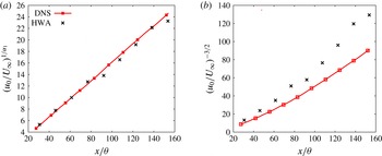
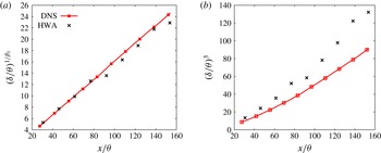
In figures 26 and 27 we plot
 $(u_{0}/U_{\infty })^{1/{\it\alpha}_{1}}$
and
 $({\it\delta}/{\it\theta})^{1/{\it\beta}_{1}}$
versus
 $x/{\it\theta}$
using the exponents given in table 2 in panels (a) and the equilibrium exponents
 ${\it\alpha}_{1}=-2/3$
and
 ${\it\beta}_{1}=1/3$
in panels (b). It is clear from these plots that
 ${\it\alpha}_{1}$
and
 ${\it\beta}_{1}$
take values that are very close to the non-equilibrium exponents
 $-1$
and
 $1/2$
, respectively. These non-equilibrium exponents are predicted by our revised George theory for
 $m=1$
. They are therefore consistent with, and presumably a consequence of, the non-equilibrium dissipation law (1.7), (2.3), (2.4) and
 $m=1$
, which seems to fit the dissipation data in figure 23(b) in the region
 $x\in [15L_{b};50L_{b}]$
.
Plots of
 $(u_{0}/U_{\infty })^{1/{\it\alpha}_{1}}$
(a) and
 $(u_{0}/U_{\infty })^{-3/2}$
(b) versus
 $x/{\it\theta}$
for
 $x\in [10L_{b};50L_{b}]$
for both the DNS and HWA cases.

Plots of
 $({\it\delta}/{\it\theta})^{1/{\it\beta}_{1}}$
(a) and
 $({\it\delta}/{\it\theta})^{3}$
(b) versus
 $x/{\it\theta}$
for
 $x\in [10L_{b};50L_{b}]$
for both the DNS and HWA cases.

We now focus on the region
 $x\in \, ]55L_{b};100L_{b} ]$
where the dissipation scaling is neither the classical equilibrium one nor (1.7), (2.3) and (2.4) with
 $m=1$
. This far-downstream range is accessible with our DNS but not in our wind tunnel experiments, and we use
 $689$
DNS data points along the streamwise direction to fit the
 $x$
dependence of the velocity deficit and the wake width in the range
 $x=57L_{b}$
to
 $x=100L_{b}$
. The position
 $x=57L_{b}$
is the closest to
 $x=55L_{b}$
for which the virtual origins
 $x_{0A2}$
and
 $x_{0B2}$
obtained by our fitting procedure are the same. The best-fitting values are reported in table 3. In agreement with the observation that the new dissipation law (1.7) taken with
 $m=1$
does not hold downstream of
 $x=55L_{b}$
(see figure 23
b), the values of the exponents
 ${\it\alpha}_{2}$
and
 ${\it\beta}_{2}$
are respectively higher and lower than the values predicted when setting
 $m=1$
in (9.2) and (9.1). Note that the values of the constants
 $A_{2}$
and
 $B_{2}$
are in very good agreement with the theory as
 $B_{2}^{-2}=2.87$
is in perfect agreement with
 $A_{2}\approx B_{2}^{-2}$
.
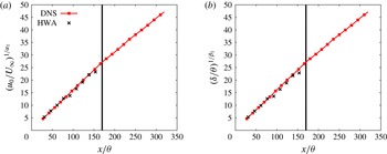
The fairly abrupt changes in power laws are manifest in figure 28 where
 $(u_{0}/U_{\infty })^{1/{\it\alpha}_{1}}$
and
 $({\it\delta}/{\it\theta})^{1/{\it\beta}_{1}}$
are plotted versus
 $x/{\it\theta}$
in the entire range
 $x\in [10L_{b};100L_{b}]$
. The well-defined linear relationships already seen in figures 26 and 27 are of course found again between
 $x=10L_{b}$
and
 $x=55L_{b}$
, but a clearly different evolution is observed for
 $x>55L_{b}$
.


Plots of
 $(u_{0}/U_{\infty })^{1/{\it\alpha}_{1}}$
(a) and
 $({\it\delta}/{\it\theta})^{1/{\it\beta}_{1}}$
(b) versus
 $x/{\it\theta}$
for
 $x\in [10L_{b};100L_{b}]$
for the DNS case. The black vertical line corresponds to
 $x=55L_{b}$
. The experimental data are included for illustration purposes for
 $x\in [10L_{b};50L_{b}]$
.

The question arises whether the exponents
 ${\it\alpha}_{2}$
and
 ${\it\beta}_{2}$
can be explained by our new predictions (9.2) and (9.1) where
 ${\it\alpha}=-2{\it\beta}=-2(1+m)/(3+m)$
. In other words, could the wake laws observed in the range
 $x\in \, ]57L_{b};100L_{b} ]$
be accountable to a dissipation law
 $C_{{\it\epsilon}}\sim (\mathit{Re}_{G}^{m}/\mathit{Re}_{l}^{m})$
? The value of
 $m$
that corresponds to our observed
 ${\it\alpha}_{2}=-0.81$
is
 $m=0.36$
, but very small uncertainties in
 ${\it\alpha}$
give rise to high uncertainties in
 $m$
at such values of
 $m$
. For example, a 40 % variation in
 $m$
above
 $m=0.36$
causes a jump of only 5 % in
 ${\it\alpha}$
. The quantity
 $(\mathit{Re}_{l}^{m}/\mathit{Re}_{G}^{m})\times C_{{\it\varepsilon}}$
exhibits a clear plateau in the range
 $x\in \, ]55L_{b};100L_{b} ]$
for
 $m=0.5$
(see figure 29 and compare it with figure 23
b) but not for
 $m=0.36$
. However, for
 $m=0.5$
,
 $-2(1+m)/(3+m)=-0.86$
, which is quite close to our observed
 ${\it\alpha}_{2}=-0.81$
and we can therefore assume that the dissipation scaling in the range
 $x\in \, ]55L_{b};100L_{b} ]$
is in fact
 $C_{{\it\epsilon}}\sim (\mathit{Re}_{G}^{1/2}/\mathit{Re}_{l}^{1/2})$
. This result suggests that the new dissipation law (1.7) still holds in the region
 $x\in \, ]55L_{b};100L_{b} ]$
but with
 $m\approx 0.5$
instead of
 $m\approx 1$
. This is confirmed by the good collapse of the dissipation profiles in this region when
 $D_{0}$
is taken to be
 $D_{0}^{NEQ2}\sim (U_{\infty }l/{\it\nu})^{1/2}(u_{0}{\it\delta}/{\it\nu})^{-1/2}K_{0}^{3/2}/{\it\delta}$
(see figure 30
b).
Streamwise variation of the product
 $(\mathit{Re}_{l}^{n}/\mathit{Re}_{G}^{m})\times C_{{\it\varepsilon}}$
for
 $m=0.5$
using the DNS data. The black vertical line corresponds to
 $x=55L_{b}$
.

In the region
 $x\in [10L_{b};50L_{b}]$
, where the velocity deficit and wake width scalings might suggest
 $m=1$
, our DNS does not return a clear collapse of the dissipation profiles when
 $D_{0}$
is taken to be
 $D_{0}^{NEQ1}\sim (U_{\infty }l/{\it\nu})^{1.0}(u_{0}{\it\delta}/{\it\nu})^{-1.0}K_{0}^{3/2}/{\it\delta}$
(i.e.
 $m=1$
). However, the DNS value of
 ${\it\alpha}_{1}$
is not
 $-1$
but
 $-0.94$
in this region (see table 2), which corresponds to
 $m=0.77$
by virtue of
 ${\it\alpha}=-2(1+m)/(3+m)$
. If
 $D_{0}$
is taken to be
 $D_{0}^{NEQ1}\sim (U_{\infty }l/{\it\nu})^{0.77}(u_{0}{\it\delta}/{\it\nu})^{-0.77}K_{0}^{3/2}/{\it\delta}$
(i.e.
 $m=0.77$
), then a good collapse of the dissipation profiles is obtained in the range
 $x\in [30L_{b};50L_{b}]$
(see figure 30
a).
Dissipation profiles at different streamwise distances using similarity scaling with
 $D_{0}^{NEQ1}\sim (U_{\infty }l/{\it\nu})^{m}(u_{0}{\it\delta}/{\it\nu})^{-m}K_{0}^{3/2}/{\it\delta}$
for
 $m=0.77$
in the range
 $x\in [30L_{b};50L_{b}]$
(a) and with
 $D_{0}^{NEQ2}\sim (U_{\infty }l/{\it\nu})^{m}(u_{0}{\it\delta}/{\it\nu})^{-m}K_{0}^{3/2}/{\it\delta}$
for
 $m=0.5$
in the range
 $x\in [55L_{b};100L_{b}]$
(b). DNS data.

10. Summary of results
DNS and HWA measurements of a turbulent wake generated by an irregular plate have been carried out in a flow configuration comparable to the experiments of Nedić et al. (Reference Nedić, Vassilicos and Ganapathisubramani2013b ). The study focused on the assessment of the theoretical assumptions and predictions for the scaling laws of the wake’s width and the centreline velocity deficit along the streamwise direction of the flow. A central goal has been to check the consistency of the turbulence dissipation law in the wake with the wake scalings.
Our DNS shows that the isotropic surrogate
 ${\it\epsilon}_{iso}$
of the turbulent dissipation is a good approximation of the turbulent dissipation in the region
 $x\geqslant 10L_{b}$
. It also shows that the approximate streamwise mean momentum equation (5.3) is a good approximation of the mean momentum balance.
The mean velocity, Reynolds shear stress, turbulent kinetic energy and dissipation profiles have been found to become axisymmetric for
 $x\geqslant 10L_{b}$
. The mean velocity and the turbulence dissipation profiles are self-similar in the region
 $x\geqslant 10L_{b}$
, whereas the Reynolds shear stresses and turbulent kinetic energy profiles are self-similar in the region
 $x\geqslant 20L_{b}$
. At least two of the three normal Reynolds stress profiles are not self-similar in the streamwise region covered by our study, implying that the turbulence production term is not self-similar either.
Our DNS and HWA data show that the turbulent kinetic energy and the Reynolds shear stress scale together and do not scale as
 $u_{0}^{2}$
. This observation has led us to introduce the assumption of constant anisotropy, which implies that
 $K_{0}\sim R_{0}$
. This assumption and the non-equilibrium dissipation law need to be invoked to predict wake width and velocity deficit scalings except when
 $m=1$
, in which case the non-equilibrium dissipation law is enough. This approach leads to a revised George (Reference George, George and Arndt1989) theory, which yields predictions for the wake width and velocity deficit scalings in agreement with our DNS and HWA data. In particular, in the DNS region
 $x\in [10L_{b};50L_{b}]$
,
 $m\approx 0.77$
and
 ${\it\alpha}\approx 0.94$
, in agreement with our formula
 ${\it\alpha}=-2(1+m)/(3+m)$
, which relates the exponents in (9.2) and
 $C_{{\it\epsilon}}\sim \mathit{Re}_{G}^{m}/\mathit{Re}_{l}^{m}$
; and in the DNS region
 $x\in \, ]55L_{b};100L_{b} ]$
,
 $m\approx 0.5$
and
 ${\it\alpha}\approx 0.86$
, again in agreement with
 ${\it\alpha}=-2(1+m)/(3+m)$
. As the local Reynolds number drops with downstream distance, one expects non-equilibrium dissipation scalings eventually to transition to the classical dissipation scaling (see Goto & Vassilicos Reference Goto and Vassilicos2015; Vassilicos Reference Vassilicos2015) at much further downstream distances.
Acknowledgements
The authors were supported by an ERC Advanced Grant (2013–2018) awarded to J.C.V. The simulations were performed at the PDC Centre for High Performance Computing at the KTH Royal Institute of Technology (Sweden) with resources provided by the DECI-11 project FRAPLAWI (EC funding RI-312763). The authors acknowledge the UK Turbulence Consortium (EPSRC research grant no. EP/L000261/1) for access to UK supercomputing resources. The authors also thank PRACE for awarding access to the SuperMUC supercomputer based at the Leibniz-Rechenzentrum (Leibniz Supercomputing Centre) in Germany and gratefully acknowledge the valuable help from the technicians of Imperial’s Department of Aeronautics for the wind tunnel experiments.