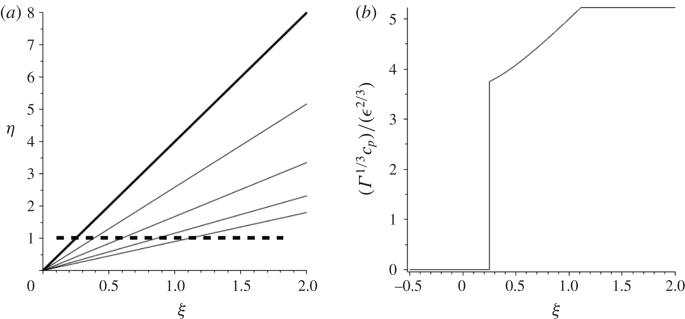
1 Introduction
The possibility that rarefaction as well as compression shocks may form in single-phase vapours was envisaged first by Bethe (Reference Bethe1942). However, his calculations based on the van der Waals equation of state indicated that the former type of shock is possible only if the ratio
 $c_{v}/R$
(where
 $c_{v}$
and
 $R$
denote the specific heat at constant volume and the universal gas constant, respectively) is larger than approximately
 $27.5$
, which he considered too large to be satisfied by real fluids. This conclusion was contested by Thompson (see Thompson Reference Thompson1971) and coworkers, who showed that this required condition for the existence of rarefaction shocks is indeed satisfied for a large number of fluorocarbon vapours. For these dense vapours, the ratio
 $c_{v}/R$
far exceeds the critical value
 $27.5$
so that the required condition for the existence of rarefaction shocks is satisfied in the general neighbourhood of the thermodynamic critical point. Thompson further showed that the type of shock capable of forming in arbitrary fluids is determined by the sign of the (non-dimensional) thermodynamic quantity
 $$\begin{eqnarray}\displaystyle & \displaystyle \unicode[STIX]{x1D6E4}(\unicode[STIX]{x1D70C},s)\equiv {\displaystyle \frac{1}{c}}{\displaystyle \frac{\unicode[STIX]{x2202}(c\unicode[STIX]{x1D70C})}{\unicode[STIX]{x2202}\unicode[STIX]{x1D70C}}}\bigg|_{s}, & \displaystyle\end{eqnarray}$$
which he referred to as the fundamental derivative of gas dynamics. In this expression for
 $\unicode[STIX]{x1D6E4}$
the local sound speed is denoted by
 $c$
and the density and entropy of the gas are denoted by
 $\unicode[STIX]{x1D70C}$
and
 $s$
, respectively. Classical gas dynamics is described by
 $\unicode[STIX]{x1D6E4}>0$
, with compressive shocks forming. If
 $\unicode[STIX]{x1D6E4}<0$
then rarefaction shocks form instead. We consider flows where
 $\unicode[STIX]{x1D6E4}$
evaluated in the free stream reference state and denoted by
 $\unicode[STIX]{x1D6E4}_{\infty }$
is small such that
 $$\begin{eqnarray}\displaystyle & \displaystyle \unicode[STIX]{x1D6E4}_{\infty }=O\left[{\displaystyle \frac{\unicode[STIX]{x1D70C}-\unicode[STIX]{x1D70C}_{\infty }}{\unicode[STIX]{x1D70C}_{\infty }}}\right], & \displaystyle\end{eqnarray}$$
i.e. of the same order as the perturbed density with respect to the free stream density
 $\unicode[STIX]{x1D70C}_{\infty }$
. There is then the possibility of
 $\unicode[STIX]{x1D6E4}(\unicode[STIX]{x1D70C},s)$
changing sign within the flow, resulting in more complex shock dynamics. In this setting of so-called mixed nonlinearity we have the possibility of compression and rarefaction shocks as well as non-classical effects such as sonic shocks and shock–fan composite structures. When
 $\unicode[STIX]{x1D6E4}$
is small its variation with density
 $\unicode[STIX]{x1D70C}$
becomes important in determining the nature of the flow and is given by the parameter
 $$\begin{eqnarray}\displaystyle & \displaystyle \unicode[STIX]{x1D6EC}(\unicode[STIX]{x1D70C},s)=\left.\unicode[STIX]{x1D70C}{\displaystyle \frac{\unicode[STIX]{x2202}\unicode[STIX]{x1D6E4}}{\unicode[STIX]{x2202}\unicode[STIX]{x1D70C}}}\right|_{s}(\unicode[STIX]{x1D70C},s). & \displaystyle\end{eqnarray}$$
For a detailed review see Kluwick (Reference Kluwick, Ben-Dor, Igra, Elperin and Lifshitz2001).
Extensive theoretical studies elaborating on the non-classical and often counterintuitive behaviour of flows with rarefaction shocks present followed the pioneering work of Thompson. These produced both results of a fundamentally theoretical character (addressing, among other issues, questions of admissibility and existence) as well as results suggesting the practical importance of rarefaction shocks, including the observation that the entropy increase and thus losses resulting from weak rarefaction shocks may be much smaller than those associated with compression shocks in perfect gases. Recognition of the early theoretical work of Bethe, Zel’dovich and Thompson on non-classical gas dynamics (see, for example, Bethe Reference Bethe1942, Zel’dovich Reference Zel’dovich1946, Thompson Reference Thompson1971) has led to the general term ‘BZT fluid’ for dense single-phase fluids exhibiting mixed nonlinearity.
In contrast to the progress in theoretical modelling of dense gas flows, experimental observations of dense gas effects – notably a rarefaction shock – have proved more elusive. Shock tube experiments designed to generate a rarefaction shock have so far failed. Studies analysing the reasons for this failure have been carried out by a number of research groups, resulting in a much better understanding of the thermodynamic properties of possible candidate fluids and identifying as such a new family of siloxanes (see Colonna, Guardone & Nannan Reference Colonna, Guardone and Nannan2007). Finally, and most importantly, the properties of vapour mixtures have recently been investigated by Guardone et al. (Reference Guardone, Colonna, Casati and Rinaldi2014), allowing for the optimisation of experimental work as well as leading to new practical applications. The results presented in this paper aim to contribute to our understanding of dense gas flows by considering an experimentally realisable flow set-up. In addition, we hope to motivate further experimental efforts to settle the long-standing question ‘do rarefaction shocks exist?’
Analytical studies of dense gas flows have in the past mainly concentrated on one-dimensional (1D) unsteady flows. In contrast to such flows, which are of strictly hyperbolic type, two-dimensional (2D) steady flows are of mixed type, i.e. hyperbolic or elliptic, depending on whether the Mach number
 $M$
is larger or smaller than one. In 1D unsteady flows it is not necessary to distinguish between the properties of shock polars and characteristics, as they agree automatically as long as changes of the entropy are negligible small. In contrast, for the case of 2D steady flows, however, the construction of shock polars has to be considered separately and their connection with characteristics deserves special attention. To provide insight into the more complex flow behaviour is the aim of the present investigation. In this connection we note that 2D steady flows have been treated already in Cramer & Tarkenton (Reference Cramer and Tarkenton1992), where the authors’ approach was predominantly a numerical investigation.
To make things as clear as possible it is necessary to keep the geometrical complexity as simple as possible. A generic problem which satisfies this requirement is given by supersonic flow past a compression/expansion ramp. It is felt that the experimental investigation of such flows provides a promising alternative to previous efforts to demonstrate the existence of non-classical flow features. Most important, there is no need for a fast opening device (punched diaphragm or valve), which is one of the key elements of shock tubes, and the resulting necessity to control 2D/3D disturbances which contaminate the intended one-dimensionality of the flow.
The paper is structured as follows: § 2 contains the concise formulation of the problem under consideration and provides the related actual scalings which form the basis of the asymptotic analysis carried out in § 3. Hodograph theory is introduced in § 4 and used to identify five regimes of qualitatively flow behaviour, which is treated in full detail. Special emphasis is placed on the geometrical interpretation of solutions which might serve as a useful guide for the selection of experimental conditions which are of relevance to both theory and practice. Finally, § 5 contains a brief summary of the results obtained as well as briefly addressing questions resulting from the – as compared to the classical case of strictly positive fundamental derivative
 $\unicode[STIX]{x1D6E4}$
– increased multiplicity of solutions for a given geometry.
2 Formulation
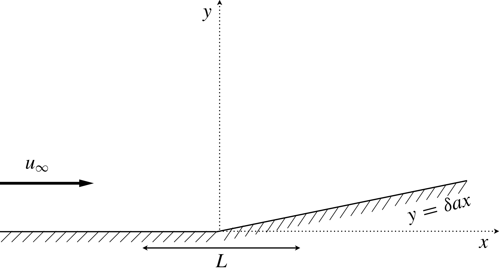
The problem considered involves steady, two-dimensional inviscid flow past a ramp (or equivalently flow past a symmetric wedge). The upstream flow ahead of the ramp has uniform speed
 $\boldsymbol{u}=(u_{\infty },0)$
aligned with the
 $x$
-axis. The corner of the ramp is located at
 $x=0$
, as shown in figure 1.
Flow geometry for a ramp located at
 $x=0$
with
 $a>0$
.

The corner geometry is
 $$\begin{eqnarray}\displaystyle & \displaystyle y=0,\quad x\leqslant 0, & \displaystyle\end{eqnarray}$$
 $$\begin{eqnarray}\displaystyle & \displaystyle y=\unicode[STIX]{x1D6FF}ax,\quad x>0, & \displaystyle\end{eqnarray}$$
where the positive parameter
 $\unicode[STIX]{x1D6FF}$
with
 $\unicode[STIX]{x1D6FF}\ll 1$
ensures that the subsequent flow generated around the corner is a small perturbation of the uniform flow and parameter
 $a=O(1)$
is used to measure the corner angle. The generated flow consists of straight shocks and wavefans providing the transition to downstream flows aligned with the boundary
 $y=\unicode[STIX]{x1D6FF}ax$
.
In Cramer & Kluwick (Reference Cramer and Kluwick1984) it is shown for BZT fluids, with
 $\unicode[STIX]{x1D6E4}$
defined by (1.1) such that
 $\unicode[STIX]{x1D6E4}\ll 1$
, and
 $\unicode[STIX]{x1D6EC}$
given by (1.3)
 $O(1)$
, that the entropy jumps across weak shocks are fourth order in the pressure (density) jump. (See also (A 15) in appendix A). In the calculations which follow, a small-disturbance transonic flow equation is derived, involving perturbed flow terms up to third order. We are therefore dealing with a consistently valid isentropic flow problem within the order of approximations employed. Similar observations can be found, for example, in Cole & Cook (Reference Cole and Cook1986) in the context of classical transonic flows. In addition, with vorticity associated with entropy gradients behind shocks assumed sufficiently small, the flow can also be assumed irrotational – a result which follows from Crocco’s vortex theorem.
Steady, irrotational, inviscid, isentropic flow in two dimensions is described by the potential equation,
 $$\begin{eqnarray}\displaystyle & \displaystyle (c^{2}-\unicode[STIX]{x1D6F7}_{x}^{2})\unicode[STIX]{x1D6F7}_{xx}+(c^{2}-\unicode[STIX]{x1D6F7}_{y}^{2})\unicode[STIX]{x1D6F7}_{yy}-2\unicode[STIX]{x1D6F7}_{x}\unicode[STIX]{x1D6F7}_{y}\unicode[STIX]{x1D6F7}_{xy}=0 & \displaystyle\end{eqnarray}$$
(see, for example, Courant & Friedrichs Reference Courant and Friedrichs1948, Cole & Cook Reference Cole and Cook1986), where
 $c$
is the sound speed and the fluid velocity
 $\boldsymbol{u}=\unicode[STIX]{x1D735}\unicode[STIX]{x1D6F7}$
. Equation (2.3) is solved subject to the kinematic boundary conditions
 $$\begin{eqnarray}\displaystyle & \displaystyle \unicode[STIX]{x1D6F7}_{y}=0,\quad \text{on }y=0,\;x\leqslant 0, & \displaystyle\end{eqnarray}$$
 $$\begin{eqnarray}\displaystyle & \displaystyle \unicode[STIX]{x1D6F7}_{y}=\unicode[STIX]{x1D6FF}a\unicode[STIX]{x1D6F7}_{x},\quad \text{on }y=\unicode[STIX]{x1D6FF}ax,\;x>0. & \displaystyle\end{eqnarray}$$
We write the velocity potential in the form
 $$\begin{eqnarray}\displaystyle & \displaystyle \unicode[STIX]{x1D6F7}=u_{\infty }x+\unicode[STIX]{x1D719}, & \displaystyle\end{eqnarray}$$
where
 $\unicode[STIX]{x1D719}$
is the deviation from a uniform upstream reference flow with velocity
 $(u_{\infty },0)$
. We assume that
 $\unicode[STIX]{x1D719}\ll 1$
in the analysis that follows.
At this stage it is useful to formulate the problem in terms of the non-dimensional variables
 $$\begin{eqnarray}\displaystyle & \displaystyle \bar{x}={\displaystyle \frac{x}{L}},\quad \bar{y}={\displaystyle \frac{y}{L}},\quad \bar{\unicode[STIX]{x1D719}}={\displaystyle \frac{\unicode[STIX]{x1D719}}{u_{\infty }L}},\quad \bar{c}={\displaystyle \frac{c}{c_{\infty }}}, & \displaystyle\end{eqnarray}$$
where
 $L$
is a representative length scale in
 $x$
over which the flow transition occurs (see figure 1) and
 $c_{\infty }=c(\unicode[STIX]{x1D70C}_{\infty },s_{\infty })$
is the sound speed of the reference flow with density
 $\unicode[STIX]{x1D70C}=\unicode[STIX]{x1D70C}_{\infty }$
and entropy
 $s=s_{\infty }$
. We assume that the flow upstream from the corner is supersonic and, without loss of generality, we can assume that the reference state is supersonic with Mach number
 $M_{\infty }=(u_{\infty }/c_{\infty })>1$
. Equation (2.3) is then formulated in terms of the perturbed potential
 $\bar{\unicode[STIX]{x1D719}}(\bar{x},\bar{y})$
as:
 $$\begin{eqnarray}\displaystyle & \displaystyle (\bar{c}^{2}-M_{\infty }^{2}-2M_{\infty }^{2}\bar{\unicode[STIX]{x1D719}}_{\bar{x}}-M_{\infty }^{2}{\bar{\unicode[STIX]{x1D719}}_{\bar{x}}}^{2})\bar{\unicode[STIX]{x1D719}}_{\bar{x}\bar{x}}+(\bar{c}^{2}-M_{\infty }^{2}{\bar{\unicode[STIX]{x1D719}}_{\bar{y}}}^{2})\bar{\unicode[STIX]{x1D719}}_{\bar{y}\bar{y}}-2M_{\infty }^{2}(1+\bar{\unicode[STIX]{x1D719}}_{\bar{x}})\bar{\unicode[STIX]{x1D719}}_{\bar{y}}\bar{\unicode[STIX]{x1D719}}_{\bar{x}\bar{y}}=0\quad & \displaystyle\end{eqnarray}$$
and the flow is taken to be in the transonic regime such that
 $$\begin{eqnarray}\displaystyle & \displaystyle |M_{\infty }^{2}-1|\ll 1. & \displaystyle\end{eqnarray}$$
As in classical dynamics of perfect gases the flow should also limit as
 $\bar{\unicode[STIX]{x1D719}}_{\bar{x}},\bar{\unicode[STIX]{x1D719}}_{\bar{y}}\rightarrow 0$
and
 $\bar{c}\rightarrow 1$
to a solution of the linear equation
 $$\begin{eqnarray}\displaystyle & \displaystyle (1-M_{\infty }^{2})\bar{\unicode[STIX]{x1D719}}_{\bar{x}\bar{x}}+\bar{\unicode[STIX]{x1D719}}_{\bar{y}\bar{y}}=0, & \displaystyle\end{eqnarray}$$
and based on this we have the scaling
 $$\begin{eqnarray}\displaystyle & \displaystyle \bar{\unicode[STIX]{x1D719}}_{\bar{y}}=O(|1-M_{\infty }^{2}|^{1/2})\bar{\unicode[STIX]{x1D719}}_{\bar{x}}, & \displaystyle\end{eqnarray}$$
a result we will use in constructing consistent approximations to equation (2.8) in the transonic regime.
3 Transonic small-disturbance equation
In this section we derive a small-disturbance equation holding in a transonic flow regime that is consistent with a small wedge angle which perturbs the upstream uniform flow. Our starting point is the potential equation given in the non-dimensional form (2.8), and to proceed we need to determine the dependence in (2.8) of
 $\bar{c}^{2}$
on the perturbed potential
 $\bar{\unicode[STIX]{x1D719}}$
. To this end we consider an expansion of the fluid pressure
 $p=p(\unicode[STIX]{x1D70C},s)$
about the uniform upstream state, yielding for the non-dimensional pressure
 $\bar{p}=(p-p_{\infty })/(\unicode[STIX]{x1D70C}_{\infty }c_{\infty }^{2})$
and density
 $\bar{\unicode[STIX]{x1D70C}}=(\unicode[STIX]{x1D70C}-\unicode[STIX]{x1D70C}_{\infty })/\unicode[STIX]{x1D70C}_{\infty }$
 $$\begin{eqnarray}\displaystyle & \displaystyle \bar{p}=\bar{\unicode[STIX]{x1D70C}}+(\unicode[STIX]{x1D6E4}_{\infty }-1)\bar{\unicode[STIX]{x1D70C}}^{2}+{\textstyle \frac{1}{3}}(3+\unicode[STIX]{x1D6EC}_{\infty })\bar{\unicode[STIX]{x1D70C}}^{3}+o(\bar{\unicode[STIX]{x1D70C}}^{3}). & \displaystyle\end{eqnarray}$$
In (3.1) the non-dimensional parameters
 $\unicode[STIX]{x1D6E4}_{\infty }$
and
 $\unicode[STIX]{x1D6EC}_{\infty }$
are
 $$\begin{eqnarray}\displaystyle & \displaystyle \unicode[STIX]{x1D6E4}_{\infty }=\unicode[STIX]{x1D6E4}(\unicode[STIX]{x1D70C}_{\infty },s_{\infty }) & \displaystyle\end{eqnarray}$$
and
 $$\begin{eqnarray}\displaystyle & \displaystyle \unicode[STIX]{x1D6EC}_{\infty }=\unicode[STIX]{x1D6EC}(\unicode[STIX]{x1D70C}_{\infty },s_{\infty }), & \displaystyle\end{eqnarray}$$
with
 $\unicode[STIX]{x1D6E4}$
and
 $\unicode[STIX]{x1D6EC}$
given by (1.1), (1.3). In the derivation of expansion (3.1) we have assumed that
 $\unicode[STIX]{x1D6E4}_{\infty }=O(\bar{\unicode[STIX]{x1D70C}})$
and
 $\unicode[STIX]{x1D6EC}_{\infty }=O(1)$
.
The parameter
 $\unicode[STIX]{x1D6E4}$
referred to by Thompson (Reference Thompson1971) as the fundamental derivative of gas dynamics plays a critical role in our understanding of gas dynamic behaviour. When
 $\unicode[STIX]{x1D6E4}$
is of fixed sign then gas dynamics is well understood qualitatively in terms of perfect gas behaviour with
 $\unicode[STIX]{x1D6E4}_{\infty }=(\unicode[STIX]{x1D6FE}+1)/2>0$
and
 $\unicode[STIX]{x1D6FE}=c_{p}/c_{v}$
, the ratio of specific heats at constant volume and constant pressure, with obvious changes for
 $\unicode[STIX]{x1D6E4}<0$
. Fluid flows where
 $\unicode[STIX]{x1D6E4}$
changes sign in the flow exhibit a more diverse range of phenomena than that observed when
 $\unicode[STIX]{x1D6E4}$
has fixed sign throughout. The possibility of
 $\unicode[STIX]{x1D6E4}$
changing sign within the flow is allowed for here by assuming that
 $\unicode[STIX]{x1D6E4}_{\infty }$
is small (of order
 $\bar{\unicode[STIX]{x1D70C}}$
). This leads to the occurrence of both stable expansion and compression shocks, and sonic shocks – shocks having a Mach number equal to the flow state upstream or downstream of the shock. Further details can be found in the review by Kluwick (Reference Kluwick and Kluwick1991).
We have, using (3.1), an expansion for
 $\bar{c}^{2}$
in the form
 $$\begin{eqnarray}\displaystyle & \displaystyle \bar{c}^{2}(\bar{\unicode[STIX]{x1D70C}})={\displaystyle \frac{\text{d}\bar{p}}{\text{d}\bar{\unicode[STIX]{x1D70C}}}}=1-2\bar{\unicode[STIX]{x1D70C}}+2\unicode[STIX]{x1D6E4}_{\infty }\bar{\unicode[STIX]{x1D70C}}+(3+\unicode[STIX]{x1D6EC}_{\infty })\bar{\unicode[STIX]{x1D70C}}^{2}+o(\bar{\unicode[STIX]{x1D70C}}^{2}). & \displaystyle\end{eqnarray}$$
Finally we use Bernoulli’s equation for steady irrotational, isentropic flow to relate the density
 $\bar{\unicode[STIX]{x1D70C}}$
arising in (3.4) to the perturbed velocity potential
 $\bar{\unicode[STIX]{x1D719}}$
.
The non-dimensional enthalpy
 $\bar{h}=(h(\unicode[STIX]{x1D70C},s)-h(\unicode[STIX]{x1D70C}_{\infty },s_{\infty }))/c_{\infty }^{2}$
satisfies Bernoulli’s equation
 $$\begin{eqnarray}\displaystyle & \displaystyle \bar{h}=-M_{\infty }^{2}\left(\bar{\unicode[STIX]{x1D719}}_{\bar{x}}+{\textstyle \frac{1}{2}}\bar{\unicode[STIX]{x1D719}}_{\bar{x}}^{2}+{\textstyle \frac{1}{2}}\bar{\unicode[STIX]{x1D719}}_{\bar{y}}^{2}\right), & \displaystyle\end{eqnarray}$$
with
 $\bar{h}$
defined as
 $$\begin{eqnarray}\displaystyle & \displaystyle \bar{h}=\int _{\unicode[STIX]{x1D70C}_{\infty }}^{\unicode[STIX]{x1D70C}}{\displaystyle \frac{\bar{c}^{2}(r)}{r}}\,\text{d}r. & \displaystyle\end{eqnarray}$$
A Taylor series expansion for
 $\bar{h}$
using the thermodynamic relationships
 $\text{d}h/\text{d}\unicode[STIX]{x1D70C}=c^{2}/\unicode[STIX]{x1D70C}$
,
 $\text{d}^{2}h/\text{d}\unicode[STIX]{x1D70C}^{2}=c^{2}(2\unicode[STIX]{x1D6E4}-3)/\unicode[STIX]{x1D70C}^{2}$
, and again adopting the core assumption of the present study
 $\unicode[STIX]{x1D6E4}_{\infty }=O(\bar{\unicode[STIX]{x1D70C}})$
and
 $\unicode[STIX]{x1D6EC}_{\infty }=O(1)$
, yields
 $$\begin{eqnarray}\displaystyle & \displaystyle \bar{h}=\bar{\unicode[STIX]{x1D70C}}-{\textstyle \frac{3}{2}}\bar{\unicode[STIX]{x1D70C}}^{2}+o(\bar{\unicode[STIX]{x1D70C}}^{2}). & \displaystyle\end{eqnarray}$$
Combining (3.5) and (3.7) we have
 $$\begin{eqnarray}\displaystyle & \displaystyle \bar{\unicode[STIX]{x1D70C}}=-\bar{\unicode[STIX]{x1D719}}_{\bar{x}}+\bar{\unicode[STIX]{x1D719}}_{\bar{x}}^{2}+O((1-M_{\infty }^{2})\bar{\unicode[STIX]{x1D719}}_{\bar{x}},\bar{\unicode[STIX]{x1D719}}_{\bar{y}}^{2}), & \displaystyle\end{eqnarray}$$
where the terms neglected can be justified a posteriori through deriving a consistent (to the same order) model equation.
We have, substituting for
 $\bar{\unicode[STIX]{x1D70C}}$
from (3.8) into (3.4),
 $$\begin{eqnarray}\displaystyle & \displaystyle \bar{c}^{2}=1+2\bar{\unicode[STIX]{x1D719}}_{\bar{x}}-2\unicode[STIX]{x1D6E4}_{\infty }\bar{\unicode[STIX]{x1D719}}_{\bar{x}}+(1+\unicode[STIX]{x1D6EC}_{\infty })\bar{\unicode[STIX]{x1D719}}_{\bar{x}}^{2}+O((1-M_{\infty }^{2})\bar{\unicode[STIX]{x1D719}}_{\bar{x}},\bar{\unicode[STIX]{x1D719}}_{\bar{y}}^{2},\unicode[STIX]{x1D6E4}_{\infty }\bar{\unicode[STIX]{x1D719}}_{\bar{x}}^{2},\bar{\unicode[STIX]{x1D719}}_{\bar{x}}^{3}). & \displaystyle\end{eqnarray}$$
With
 $\bar{c}^{2}$
given then in this form (2.8) reduces to
 $$\begin{eqnarray}\displaystyle & \displaystyle (1-M_{\infty }^{2}-2\unicode[STIX]{x1D6E4}_{\infty }\bar{\unicode[STIX]{x1D719}}_{\bar{x}}+\unicode[STIX]{x1D6EC}_{\infty }{\bar{\unicode[STIX]{x1D719}}_{\bar{x}}}^{2}+O((1-M_{\infty }^{2})\bar{\unicode[STIX]{x1D719}}_{\bar{x}},\unicode[STIX]{x1D6E4}_{\infty }\bar{\unicode[STIX]{x1D719}}_{\bar{x}}^{2},\bar{\unicode[STIX]{x1D719}}_{\bar{x}}^{3}))\bar{\unicode[STIX]{x1D719}}_{\bar{x}\bar{x}}+(1+O(\bar{\unicode[STIX]{x1D719}}_{\bar{x}},{\bar{\unicode[STIX]{x1D719}}_{\bar{y}}}^{2}))\bar{\unicode[STIX]{x1D719}}_{\bar{y}\bar{y}}=0. & \displaystyle \nonumber\\ \displaystyle & & \displaystyle\end{eqnarray}$$
The nonlinear term
 $\bar{\unicode[STIX]{x1D719}}_{y}\bar{\unicode[STIX]{x1D719}}_{\bar{x}\bar{y}}$
is
 $O((1-M_{\infty }^{2})\bar{\unicode[STIX]{x1D719}}_{\bar{x}}\bar{\unicode[STIX]{x1D719}}_{\bar{x}\bar{x}})$
and is excluded, consistent with the approximations made. We note that
 $\unicode[STIX]{x1D6E4}_{\infty }=O(\bar{\unicode[STIX]{x1D70C}})$
,
 $\unicode[STIX]{x1D6EC}_{\infty }=O(1)$
in (3.10), as assumed previously, and a balance between linear and nonlinear terms requires that
 $$\begin{eqnarray}\displaystyle & \displaystyle 1-M_{\infty }^{2}=O(\bar{\unicode[STIX]{x1D719}}_{\bar{x}}^{2}). & \displaystyle\end{eqnarray}$$
The problem formulated in (2.3), (2.4) and (2.5) has now been reduced to solving
 $$\begin{eqnarray}\displaystyle & \displaystyle (1-M_{\infty }^{2}-2\unicode[STIX]{x1D6E4}_{\infty }\bar{\unicode[STIX]{x1D719}}_{\bar{x}}+\unicode[STIX]{x1D6EC}_{\infty }{\bar{\unicode[STIX]{x1D719}}_{\bar{x}}}^{2})\bar{\unicode[STIX]{x1D719}}_{\bar{x}\bar{x}}+\bar{\unicode[STIX]{x1D719}}_{\bar{y}\bar{y}}=0, & \displaystyle\end{eqnarray}$$
with from (2.4), (2.5) and (2.6) consistent approximate boundary conditions prescribed now on
 $\bar{y}=0$
by
 $$\begin{eqnarray}\displaystyle & \displaystyle \bar{\unicode[STIX]{x1D719}}_{\bar{y}}=0,\quad \bar{x}\leqslant 0, & \displaystyle\end{eqnarray}$$
 $$\begin{eqnarray}\displaystyle & \displaystyle \bar{\unicode[STIX]{x1D719}}_{\bar{y}}=\unicode[STIX]{x1D6FF}a,\quad \bar{x}>0. & \displaystyle\end{eqnarray}$$
Details of the derivation presented here and leading to (3.12) can be found in Cramer & Tarkenton (Reference Cramer and Tarkenton1992) for transonic flow over slender wings. An extension, again in the context of slender wings, to include flows where
 $\unicode[STIX]{x1D6E4}_{\infty }=O(\bar{\unicode[STIX]{x1D70C}}^{2}),\unicode[STIX]{x1D6EC}_{\infty }=O(\bar{\unicode[STIX]{x1D70C}})$
is given in Kluwick (Reference Kluwick1993), Schnerr & Molokov (Reference Schnerr and Molokov1994).
With the scalings given by (2.11), (3.11) we can determine from (3.13), (3.14) the order estimates
 $$\begin{eqnarray}\displaystyle & \displaystyle 1-M_{\infty }^{2}=O(\unicode[STIX]{x1D6FF}),\quad \bar{\unicode[STIX]{x1D719}}_{\bar{y}}=O(\unicode[STIX]{x1D6FF}),\quad \bar{\unicode[STIX]{x1D719}}_{\bar{x}}=O(\unicode[STIX]{x1D6FF}^{1/2}) & \displaystyle\end{eqnarray}$$
relating the flow generated to the boundary conditions imposed. This suggests an alternative approach to the derivation of (3.12). Instead of beginning with a potential flow formulation we could start with the Euler equations of motion and consider flows which represent small disturbances of uniform flow in the transonic regime given by
 $|1-M_{\infty }^{2}|=O(\unicode[STIX]{x1D6FF})$
, where
 $\unicode[STIX]{x1D6FF}\ll 1$
. Then the scalings given in (3.15) would arise as a formal distinguished asymptotic limit of the Euler equations and boundary conditions. The result once again would be (3.12). This is the approach used, for example, in Cole & Cook (Reference Cole and Cook1986) for classical transonic flows. An important difference, however, is observed between the classical scalings and those for BZT fluids. In the classical case
 $|1-M_{\infty }^{2}|=O(\unicode[STIX]{x1D6FF}^{2/3})$
, whereas the transonic regime for BZT fluids is more restrictive, with
 $|1-M_{\infty }^{2}|=O(\unicode[STIX]{x1D6FF})$
.
The local Mach number for the flow is given by
 $$\begin{eqnarray}\displaystyle & \displaystyle M^{2}=M_{\infty }^{2}{\displaystyle \frac{(1+\unicode[STIX]{x1D719}_{\bar{x}})^{2}+\unicode[STIX]{x1D719}_{\bar{y}}^{2}}{\bar{c}^{2}}} & \displaystyle\end{eqnarray}$$
and using (2.7), (3.9) and (3.11), (3.15) we have
 $$\begin{eqnarray}\displaystyle & \displaystyle M^{2}=M_{\infty }^{2}+2\unicode[STIX]{x1D6E4}_{\infty }\bar{\unicode[STIX]{x1D719}}_{\bar{x}}-\unicode[STIX]{x1D6EC}_{\infty }{\bar{\unicode[STIX]{x1D719}}_{\bar{x}}}^{2}+o({\bar{\unicode[STIX]{x1D719}}_{\bar{x}}}^{2},|M_{\infty }^{2}-1|). & \displaystyle\end{eqnarray}$$
The small-disturbance transonic approximation (3.12) of the equations of gas dynamics can then be written in the familiar form
 $$\begin{eqnarray}\displaystyle & \displaystyle (1-M^{2})\bar{\unicode[STIX]{x1D719}}_{\bar{x}\bar{x}}+\bar{\unicode[STIX]{x1D719}}_{\bar{y}\bar{y}}=0, & \displaystyle\end{eqnarray}$$
an equation which changes type as
 $M^{2}-1$
changes sign.
From (3.17) we see that sonic conditions
 $(M=1)$
arise in downstream flows satisfying
 $$\begin{eqnarray}\displaystyle & \displaystyle \bar{\unicode[STIX]{x1D719}}_{\bar{x}}={\displaystyle \frac{\unicode[STIX]{x1D6E4}_{\infty }}{\unicode[STIX]{x1D6EC}_{\infty }}}\pm {\displaystyle \frac{1}{\unicode[STIX]{x1D6EC}_{\infty }}}\sqrt{\unicode[STIX]{x1D6E4}_{\infty }^{2}+\unicode[STIX]{x1D6EC}_{\infty }(M_{\infty }^{2}-1)} & \displaystyle\end{eqnarray}$$
and we assume
 $M_{\infty }^{2}>1$
. It is clear then that two sonic values for
 $\bar{\unicode[STIX]{x1D719}}_{\bar{x}}$
exist for
 $\unicode[STIX]{x1D6EC}_{\infty }>0$
while for
 $\unicode[STIX]{x1D6EC}_{\infty }<0$
we have purely supersonic flow if
 $$\begin{eqnarray}\displaystyle & \displaystyle M_{\infty }>\left(1-{\displaystyle \frac{\unicode[STIX]{x1D6E4}_{\infty }^{2}}{\unicode[STIX]{x1D6EC}_{\infty }}}\right)^{1/2}. & \displaystyle\end{eqnarray}$$
In contrast, the case
 $\unicode[STIX]{x1D6EC}_{\infty }=0$
, which corresponds to classical gas dynamics, has only one sonic point. For sufficiently large, but negative, values of
 $\bar{\unicode[STIX]{x1D719}}_{\bar{x}}$
the flow is always subsonic.
The steady transonic small-disturbance equation (3.18) is hyperbolic for supersonic flows
 $M>1$
. With
 $y$
as a ‘time-like’ variable the disturbance in
 $y>0$
is generated along characteristics propagating away from the corner boundary surfaces. These characteristics are integral curves of
 $$\begin{eqnarray}\displaystyle & \displaystyle {\displaystyle \frac{\text{d}\bar{x}}{\text{d}\bar{y}}}=\pm \sqrt{-{\displaystyle \frac{\text{d}J}{\text{d}\bar{\unicode[STIX]{x1D719}}_{\bar{x}}}}},\quad J=(1-M_{\infty }^{2})\bar{\unicode[STIX]{x1D719}}_{\bar{x}}-\unicode[STIX]{x1D6E4}_{\infty }\bar{\unicode[STIX]{x1D719}}_{\bar{x}}^{2}+{\displaystyle \frac{\unicode[STIX]{x1D6EC}_{\infty }}{3}}{\bar{\unicode[STIX]{x1D719}}_{\bar{x}}}^{3}, & \displaystyle\end{eqnarray}$$
where
 $$\begin{eqnarray}\displaystyle & \displaystyle M^{2}-1=-{\displaystyle \frac{\text{d}J}{\text{d}\bar{\unicode[STIX]{x1D719}}_{\bar{x}}}}. & \displaystyle\end{eqnarray}$$
Explicit solutions to (3.21) can be found in Schnerr & Molokov (Reference Schnerr and Molokov1994) with applications to vortex flow, Ringleb flow and jet flows. In introducing the function
 $J(\bar{\unicode[STIX]{x1D719}}_{\bar{x}})$
in (3.21) we make the connection to the 1D evolution problem, where
 $J$
is the nonlinear flux function considered by Kluwick (Reference Kluwick and Kluwick1991), and the internal transonic flow analysis of Kluwick (Reference Kluwick1993), where
 $J$
is the density of the perturbation mass flux. The nonlinear dependence of
 $J$
on
 $\bar{\unicode[STIX]{x1D719}}_{\bar{x}}$
leads to possible intersections of characteristics, indicating the occurrence of shock discontinuities in the flow. Across the shock, flow quantities are discontinuous and a selection criterion is required to exclude those discontinuities that are not physically meaningful. In appendix A we show that valid discontinuities satisfy (A 28), namely
 $$\begin{eqnarray}\displaystyle & \displaystyle \left.-{\displaystyle \frac{\text{d}J}{\text{d}\bar{\unicode[STIX]{x1D719}}_{\bar{x}}}}\right|_{1}\geqslant -{\displaystyle \frac{[J]}{[\bar{\unicode[STIX]{x1D719}}_{\bar{x}}]}}\geqslant \left.-{\displaystyle \frac{\text{d}J}{\text{d}\bar{\unicode[STIX]{x1D719}}_{\bar{x}}}}\right|_{2}, & \displaystyle\end{eqnarray}$$
which provides an ordering of characteristic slopes ahead of and behind the shock (
 $-\text{d}J/\text{d}\bar{\unicode[STIX]{x1D719}}_{\bar{x}}|_{1,2}$
) to the shock slope (
 $-[J]/[\bar{\unicode[STIX]{x1D719}}_{\bar{x}}]$
), stated here for right running waves only (positive sign in (3.21)). In (3.23), subscripts
 $1$
and
 $2$
refer to states upstream and downstream of the shock and
 $[Q]=Q_{2}-Q_{1}$
for any flow quantity
 $Q$
. We note that the condition (3.23) relates the shock speed to the wave speeds upstream and downstream of the shock front, and is therefore commonly referred to as a ‘speed’ ordering condition. These inequalities also play the same role in steady transonic flows that the entropy conditions play in time-dependent hyperbolic conservation laws. We note that (3.23) is valid only for
 $-\text{d}J/\text{d}\bar{\unicode[STIX]{x1D719}}_{\bar{x}}|_{1,2}=(M^{2}-1)|_{1,2}\geqslant 0$
, i.e. supersonic upstream and downstream states.
Qualitatively different solutions are identified with parameter regimes in the space
 $(M_{\infty },\unicode[STIX]{x1D6FF}a,\unicode[STIX]{x1D6E4}_{\infty },\unicode[STIX]{x1D6EC}_{\infty })$
. This can be reduced to essentially a 2D parameter space through the scalings
 $$\begin{eqnarray}\displaystyle & \displaystyle \bar{\unicode[STIX]{x1D719}}={\displaystyle \frac{\unicode[STIX]{x1D6FF}^{2/3}}{\unicode[STIX]{x1D6E4}_{\infty }^{1/3}}}\unicode[STIX]{x1D713},\quad \bar{x}=\unicode[STIX]{x1D709},\quad \bar{y}={\displaystyle \frac{\unicode[STIX]{x1D702}}{\unicode[STIX]{x1D6FF}^{1/3}|\unicode[STIX]{x1D6E4}_{\infty }|^{1/3}}} & \displaystyle\end{eqnarray}$$
introduced by Cramer & Tarkenton (Reference Cramer and Tarkenton1992). Substituting (3.24) into (3.12)–(3.14) we have
 $$\begin{eqnarray}\displaystyle & \displaystyle (-K_{1}-2\unicode[STIX]{x1D713}_{\unicode[STIX]{x1D709}}+K_{2}\unicode[STIX]{x1D713}_{\unicode[STIX]{x1D709}}^{2})\unicode[STIX]{x1D713}_{\unicode[STIX]{x1D709}\unicode[STIX]{x1D709}}+\unicode[STIX]{x1D713}_{\unicode[STIX]{x1D702}\unicode[STIX]{x1D702}}=0, & \displaystyle\end{eqnarray}$$
where
 $K_{1}$
,
 $K_{2}$
are the similarity parameters
 $$\begin{eqnarray}\displaystyle & \displaystyle K_{1}={\displaystyle \frac{M_{\infty }^{2}-1}{(\unicode[STIX]{x1D6FF}\unicode[STIX]{x1D6E4}_{\infty })^{2/3}}},\quad K_{2}={\displaystyle \frac{\unicode[STIX]{x1D6FF}^{2/3}\unicode[STIX]{x1D6EC}_{\infty }}{\unicode[STIX]{x1D6E4}_{\infty }^{4/3}}}. & \displaystyle\end{eqnarray}$$
Equation (3.25) exhibits quadratic and cubic nonlinearity, frequently summarised as mixed nonlinearity.
The boundary conditions (3.13), (3.14), now on
 $\unicode[STIX]{x1D702}=0$
, become
 $$\begin{eqnarray}\displaystyle & \displaystyle \unicode[STIX]{x1D713}_{\unicode[STIX]{x1D702}}=0,\quad \unicode[STIX]{x1D709}\leqslant 0, & \displaystyle\end{eqnarray}$$
 $$\begin{eqnarray}\displaystyle & \displaystyle \unicode[STIX]{x1D713}_{\unicode[STIX]{x1D702}}=a\operatorname{sgn}(\unicode[STIX]{x1D6E4}_{\infty }),\quad \unicode[STIX]{x1D709}>0. & \displaystyle\end{eqnarray}$$
Some obvious comments can be made about the transformed equations (3.25)–(3.28): firstly,
 $K_{1}$
is positive for supersonic upstream flows and is a rescaled transonic similarity parameter that arises in classical flows, and
 $K_{2}$
then expresses the relative importance of cubic and quadratic nonlinearity – changing sign with
 $\unicode[STIX]{x1D6EC}_{\infty }$
. Secondly the sign of
 $\unicode[STIX]{x1D6E4}_{\infty }$
only enters into the boundary condition (3.28), and changing the sign of
 $\unicode[STIX]{x1D6E4}_{\infty }$
is equivalent to changing the sign of
 $a$
, i.e. switching from a concave to convex corner or vice versa. Finally, there are two sonic points, in general, where (3.25) changes type from hyperbolic to elliptic.
The characteristics and shock slope ordering condition (3.23) transformed into variables given by (3.24), (3.26) yields
 $$\begin{eqnarray}\displaystyle & \displaystyle \left.-{\displaystyle \frac{\text{d}j}{\text{d}\unicode[STIX]{x1D713}_{\unicode[STIX]{x1D709}}}}\right|_{1}\geqslant -{\displaystyle \frac{[j]}{[\unicode[STIX]{x1D713}_{\unicode[STIX]{x1D709}}]}}\geqslant \left.-{\displaystyle \frac{\text{d}j}{\text{d}\unicode[STIX]{x1D713}_{\unicode[STIX]{x1D709}}}}\right|_{2}, & \displaystyle\end{eqnarray}$$
with
 $$\begin{eqnarray}\displaystyle & \displaystyle j=-K_{1}\unicode[STIX]{x1D713}_{\unicode[STIX]{x1D709}}-\unicode[STIX]{x1D713}_{\unicode[STIX]{x1D709}}^{2}+{\displaystyle \frac{K_{2}}{3}}\unicode[STIX]{x1D713}_{\unicode[STIX]{x1D709}}^{3} & \displaystyle\end{eqnarray}$$
and we note that (3.29) is independent of the sign of
 $\unicode[STIX]{x1D6E4}_{\infty }$
.
When the flow is supersonic (
 $\text{d}j/\text{d}\unicode[STIX]{x1D713}_{\unicode[STIX]{x1D709}}<0$
) characteristic curves given by (3.21) transform to
 $$\begin{eqnarray}\displaystyle & \displaystyle {\displaystyle \frac{\text{d}\unicode[STIX]{x1D709}}{\text{d}\unicode[STIX]{x1D702}}}=\pm \sqrt{-{\displaystyle \frac{\text{d}j}{\text{d}\unicode[STIX]{x1D713}_{\unicode[STIX]{x1D709}}}}}. & \displaystyle\end{eqnarray}$$
In (3.31) the expression
 $-\text{d}j/\text{d}\unicode[STIX]{x1D713}_{\unicode[STIX]{x1D709}}$
is the scaled Mach number given by
 $$\begin{eqnarray}\displaystyle & \displaystyle {\displaystyle \frac{2(M-1)}{(\unicode[STIX]{x1D6FF}\unicode[STIX]{x1D6E4}_{\infty })^{2/3}}}\approx K_{1}+2\unicode[STIX]{x1D713}_{\unicode[STIX]{x1D709}}-K_{2}\unicode[STIX]{x1D713}_{\unicode[STIX]{x1D709}}^{2}=-{\displaystyle \frac{\text{d}j}{\text{d}\unicode[STIX]{x1D713}_{\unicode[STIX]{x1D709}}}}. & \displaystyle\end{eqnarray}$$
We observe from (3.31), (3.32) that in contrast to the classical case
 $K_{2}=0$
characteristic slopes do not vary monotonically with
 $\unicode[STIX]{x1D713}_{\unicode[STIX]{x1D709}}$
. As we have already seen for (3.18) there are two flows in general corresponding to sonic conditions
 $M=1$
. For (3.25) these flows, for
 $K_{2}>-1/K_{1}$
, satisfy
 $$\begin{eqnarray}\displaystyle & \displaystyle {\unicode[STIX]{x1D713}_{\unicode[STIX]{x1D709}}}_{sonic}={\displaystyle \frac{1}{K_{2}}}\pm {\displaystyle \frac{1}{K_{2}}}\sqrt{1+K_{1}K_{2}}. & \displaystyle\end{eqnarray}$$
When
 $K_{2}=-1/K_{1}$
there is a single sonic point at
 ${\unicode[STIX]{x1D713}_{\unicode[STIX]{x1D709}}}_{sonic}=-K_{1}$
, and if
 $K_{2}<-1/K_{1}$
the flow is never sonic.
4 Hodograph plane
A convenient formulation of (3.25) is
 $$\begin{eqnarray}\displaystyle & \displaystyle (-K_{1}-2\tilde{u} +K_{2}\tilde{u} ^{2})\tilde{u} _{\unicode[STIX]{x1D709}}+\tilde{v}_{\unicode[STIX]{x1D702}}=0, & \displaystyle\end{eqnarray}$$
 $$\begin{eqnarray}\displaystyle & \displaystyle \tilde{u} _{\unicode[STIX]{x1D702}}-\tilde{v}_{\unicode[STIX]{x1D709}}=0, & \displaystyle\end{eqnarray}$$
with
 $\unicode[STIX]{x1D713}_{\unicode[STIX]{x1D709}}=\tilde{u}$
,
 $\unicode[STIX]{x1D713}_{\unicode[STIX]{x1D702}}=\tilde{v}$
and
 $\tilde{u} ,\tilde{v}$
are then perturbed velocity components in similarity variables. We consider the functions
 $\tilde{u} (\unicode[STIX]{x1D709},\unicode[STIX]{x1D702})$
,
 $\tilde{v}(\unicode[STIX]{x1D709},\unicode[STIX]{x1D702})$
as a mapping
 $L:(\unicode[STIX]{x1D709},\unicode[STIX]{x1D702})\mapsto (\tilde{u} ,\tilde{v})$
which is locally invertible providing
 $$\begin{eqnarray}\displaystyle & \displaystyle {\displaystyle \frac{\unicode[STIX]{x2202}(\tilde{u} ,\tilde{v})}{\unicode[STIX]{x2202}(\unicode[STIX]{x1D709},\unicode[STIX]{x1D702})}}=\tilde{u} _{\unicode[STIX]{x1D709}}\tilde{v}_{\unicode[STIX]{x1D702}}-\tilde{u} _{\unicode[STIX]{x1D702}}\tilde{v}_{\unicode[STIX]{x1D709}}\neq 0. & \displaystyle\end{eqnarray}$$
Applying the inverse map
 $L^{-1}$
we have the so-called hodograph system
 $$\begin{eqnarray}\displaystyle & \displaystyle (-K_{1}-2\tilde{u} +K_{2}\tilde{u} ^{2})\unicode[STIX]{x1D702}_{\tilde{v}}+\unicode[STIX]{x1D709}_{\tilde{u} }=0, & \displaystyle\end{eqnarray}$$
 $$\begin{eqnarray}\displaystyle & \displaystyle \unicode[STIX]{x1D709}_{\tilde{v}}-\unicode[STIX]{x1D702}_{\tilde{u} }=0, & \displaystyle\end{eqnarray}$$
which can be written as the second-order linear (generalised) Tricomi equation
 $$\begin{eqnarray}\displaystyle & \displaystyle (-K_{1}-2\tilde{u} +K_{2}\tilde{u} ^{2})\unicode[STIX]{x1D702}_{\tilde{v}\tilde{v}}+\unicode[STIX]{x1D702}_{\tilde{u} \tilde{u} }=0. & \displaystyle\end{eqnarray}$$
Details of the hodograph method can be found in, for example, Cole & Cook (Reference Cole and Cook1986) applied to the classical case
 $K_{2}=0$
. Solutions to (4.6) have been investigated by Schnerr & Molokov (Reference Schnerr and Molokov1994) for vortex, jet and Ringleb flows.
In the hyperbolic domain where
 $K_{1}+2\tilde{u} -K_{2}\tilde{u} ^{2}>0$
, which corresponds to supersonic flow in the physical domain, characteristics of (4.6) are given by the integral curves of
 $$\begin{eqnarray}\displaystyle & \displaystyle {\displaystyle \frac{\text{d}\tilde{v}}{\text{d}\tilde{u} }}=\pm \sqrt{K_{1}+2\tilde{u} -K_{2}\tilde{u} ^{2}}=\pm \sqrt{-{\displaystyle \frac{\text{d}j}{\text{d}\tilde{u} }}} & \displaystyle\end{eqnarray}$$
and map onto the physical characteristics (3.31) with the two sets of characteristics orthogonal to each other. Equation (4.7) is straightforward to integrate and the details are not presented here.
We now consider the problem of constructing solutions for the corner flow geometry. Without loss of generality we can assume the perturbed flow
 $\tilde{u} =0$
,
 $\tilde{v}=0$
upstream of the corner. (Translations in
 $\tilde{u}$
can be incorporated through redefining
 $u_{\infty }$
).
Flows in the physical plane can be constructed and understood from the corresponding solutions in the hodograph plane. This construction is implemented in § 4.1 for shock solutions and in § 4.2 for simple wave solutions. These basic building blocks consist of solutions propagating on characteristic curves and across shock jumps. It is well known in supersonic flows that uniform flow states (i.e. the upstream and downstream states for corner geometry) can be connected either by shock solutions, so-called ‘simple wave’ solutions or combinations of both.
4.1 Shock waves
We consider all possible downstream states connected by a shock to a given upstream state. This curve in the
 $(\tilde{u} ,\tilde{v})$
hodograph plane is known as the shock polar and extends well-known results for the classical problem. Integrating (3.12) across the shock surface
 $\bar{x}=S(\bar{y})$
yields the shock jump conditions (A 22), (A 23). Eliminating the shock slope
 $\text{d}S/\text{d}\bar{y}$
gives the shock polar
 $$\begin{eqnarray}\displaystyle & \displaystyle [v]^{2}+[J][u]=0, & \displaystyle\end{eqnarray}$$
with
 $v=\bar{\unicode[STIX]{x1D719}}_{\bar{y}}$
and
 $u=\bar{\unicode[STIX]{x1D719}}_{\bar{x}}$
.
In the similarity variables of (3.24), (3.26), equation (4.8) transforms to
 $$\begin{eqnarray}\displaystyle & \displaystyle [\tilde{v}]^{2}+[j][\tilde{u} ]=0,\quad j=-K_{1}\tilde{u} -\tilde{u} ^{2}+{\displaystyle \frac{K_{2}}{3}}\tilde{u} ^{3}. & \displaystyle\end{eqnarray}$$
It is more revealing to write (4.9) in the form
 $$\begin{eqnarray}\displaystyle & \displaystyle {\displaystyle \frac{[\tilde{v}]}{[\tilde{u} ]}}=\pm \sqrt{-{\displaystyle \frac{[j]}{[\tilde{u} ]}}}. & \displaystyle\end{eqnarray}$$
The shock slope is given in the physical domain by (A 23), which in similarity variables becomes
 $$\begin{eqnarray}\displaystyle & \displaystyle {\displaystyle \frac{\text{d}\unicode[STIX]{x1D702}}{\text{d}\unicode[STIX]{x1D709}}}=\mp {\displaystyle \frac{1}{\sqrt{-{\displaystyle \frac{[j]}{[\tilde{u} ]}}}}}. & \displaystyle\end{eqnarray}$$
We observe then the useful geometric construction that the slope of the chord
 $[\tilde{v}]/[\tilde{u} ]$
is orthogonal to the shock slope with appropriately chosen signs.
4.2 Simple waves
We consider the formulation of the problem given by (4.1), (4.2) and look for solutions described by a single coordinate
 $r=r(\unicode[STIX]{x1D709},\unicode[STIX]{x1D702})$
. Equations (4.1), (4.2) are transformed to
 $$\begin{eqnarray}\displaystyle & \displaystyle (-K_{1}-2\tilde{u} +K_{2}\tilde{u} ^{2}){\displaystyle \frac{\text{d}\tilde{u} }{\text{d}r}}r_{\unicode[STIX]{x1D709}}+{\displaystyle \frac{\text{d}\tilde{v}}{\text{d}r}}r_{\unicode[STIX]{x1D702}}=0, & \displaystyle\end{eqnarray}$$
 $$\begin{eqnarray}\displaystyle & \displaystyle {\displaystyle \frac{\text{d}\tilde{u} }{\text{d}r}}r_{\unicode[STIX]{x1D702}}-{\displaystyle \frac{\text{d}\tilde{v}}{\text{d}r}}r_{\unicode[STIX]{x1D709}}=0. & \displaystyle\end{eqnarray}$$
Solutions exist providing
 $\tilde{u}$
and
 $\tilde{v}$
vary with
 $r$
according to
 $$\begin{eqnarray}\displaystyle & \displaystyle (-K_{1}-2\tilde{u} +K_{2}\tilde{u} ^{2})\left({\displaystyle \frac{\text{d}\tilde{u} }{\text{d}r}}\right)^{2}+\left({\displaystyle \frac{\text{d}\tilde{v}}{\text{d}r}}\right)^{2}=0, & \displaystyle\end{eqnarray}$$
which is possible only if the flow throughout the wave is supersonic. Equation (4.14) provides the image of the simple wave in the hodograph plane
 $$\begin{eqnarray}\displaystyle & \displaystyle {\displaystyle \frac{\text{d}\tilde{v}}{\text{d}r}}=\pm \sqrt{K_{1}+2\tilde{u} -K_{2}\tilde{u} ^{2}}{\displaystyle \frac{\text{d}\tilde{u} }{\text{d}r}}, & \displaystyle\end{eqnarray}$$
and comparing with (4.7) we see that the mapping is to a single characteristic in the hodograph plane with
 $r$
now labelling position along the characteristic curve. This is consistent with showing that
 $\unicode[STIX]{x2202}(\tilde{u} ,\tilde{v})/\unicode[STIX]{x2202}(\unicode[STIX]{x1D709},\unicode[STIX]{x1D702})=0$
for simple waves and the hodograph mapping is then not invertible. Each point on the identified characteristic curve labelled by parameter
 $r$
corresponds to a straight line characteristic in the physical plane with slope
 $$\begin{eqnarray}\displaystyle & \displaystyle \left.{\displaystyle \frac{\text{d}\unicode[STIX]{x1D702}}{\text{d}\unicode[STIX]{x1D709}}}\right|_{r}=-{\displaystyle \frac{r_{\unicode[STIX]{x1D709}}}{r_{\unicode[STIX]{x1D702}}}}=\mp {\displaystyle \frac{1}{\sqrt{K_{1}+2\tilde{u} (r)-K_{2}\tilde{u} (r)^{2}}}}=\mp {\displaystyle \frac{1}{\left.\sqrt{-{\displaystyle \frac{\text{d}j}{\text{d}\tilde{u} }}}\right|_{r}}}. & \displaystyle\end{eqnarray}$$
If all these straight characteristics pass through a single point then the wave is called a centred simple wave. The curved cross-characteristics in the physical plane all map onto the single characteristic in the hodograph plane and carry no propagating signal.
A useful geometric interpretation in the hodograph plane is based on recognising that the slope (4.16) is orthogonal to the mapped characteristic, which at
 $r$
has slope
 $$\begin{eqnarray}\displaystyle & \displaystyle \left.{\displaystyle \frac{\text{d}\tilde{v}}{\text{d}\tilde{u} }}\right|_{r}=\pm \sqrt{K_{1}+2\tilde{u} (r)-K_{2}\tilde{u} (r)^{2}}=\left.\pm \sqrt{-{\displaystyle \frac{\text{d}j}{\text{d}\tilde{u} }}}\right|_{r}. & \displaystyle\end{eqnarray}$$
4.3 Hodograph representation of flows
The nature in the hodograph plane of these elemental solutions (shock waves and simple waves) – both their existence and structure – depends on the function
 $-j(\tilde{u} )$
as can be seen from (4.10) and (4.17). In the context of upstream supersonic flow with
 $K_{1}>0$
we can identify five parameter ranges of
 $K_{2}$
corresponding to qualitatively different flow scenarios. These parameter ranges are
 $K_{2}>0$
,
 $K_{2}=0$
,
 $-(3/4K_{1})<K_{2}<0$
,
 $-(1/K_{1})<K_{2}<-(3/4K_{1})$
and
 $K_{2}<-1/K_{1}$
. With the definition of
 $K_{2}$
in (3.26) we can relate variations in
 $K_{2}$
to the relative effect of cubic nonlinearity introduced through the parameter
 $\unicode[STIX]{x1D6EC}_{\infty }$
in
 $-j(\tilde{u} )$
. In physical terms this relates to changes in the fluid properties of the upstream state.
We begin with a consideration of the case
 $K_{2}=0$
, which corresponds to the classical perfect gas case if
 $\unicode[STIX]{x1D6E4}>0$
, where the results and analysis are well known.
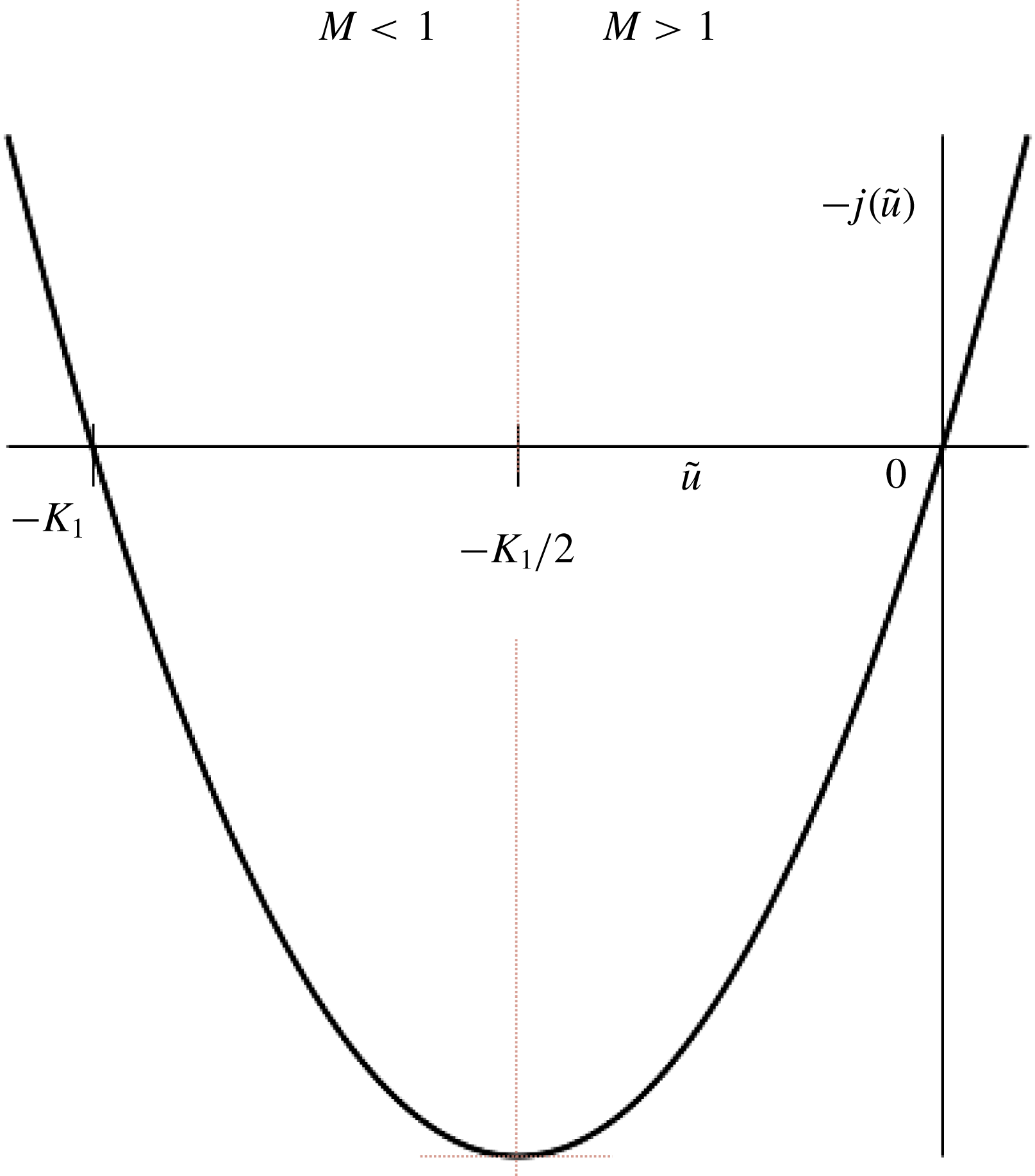
The function
 $-j(\tilde{u} )$
for
 $K_{1}>0$
,
 $K_{2}=0$
.

4.3.1 Case
 $K_{1}>0$
,
$K_{2}=0$


We first make some observations based on the plot of
 $-j(\tilde{u} )$
in figure 2. For the downstream state
 $\tilde{u} =-K_{1}/2$
, where
 $-\text{d}j/\text{d}\tilde{u} =0$
, the flow is sonic (from (3.32)), supersonic for
 $\tilde{u} >-K_{1}/2$
and subsonic for
 $\tilde{u} <-K_{1}/2$
. Shock solutions can connect the upstream state
 $\tilde{u} =0$
to downstream states only in the interval
 $-K_{1}<\tilde{u} <0$
, where
 $-j(\tilde{u} )$
is negative (readily deduced from (4.10)). The shock solutions satisfy the jump inequalities (3.29). Positive downstream states
 $\tilde{u} >0$
can be reached through a continuous transition from
 $\tilde{u} =0$
and describes continuously accelerated flows. Within the context of small-disturbance theory there is no limit to the strength of the transitions generated.
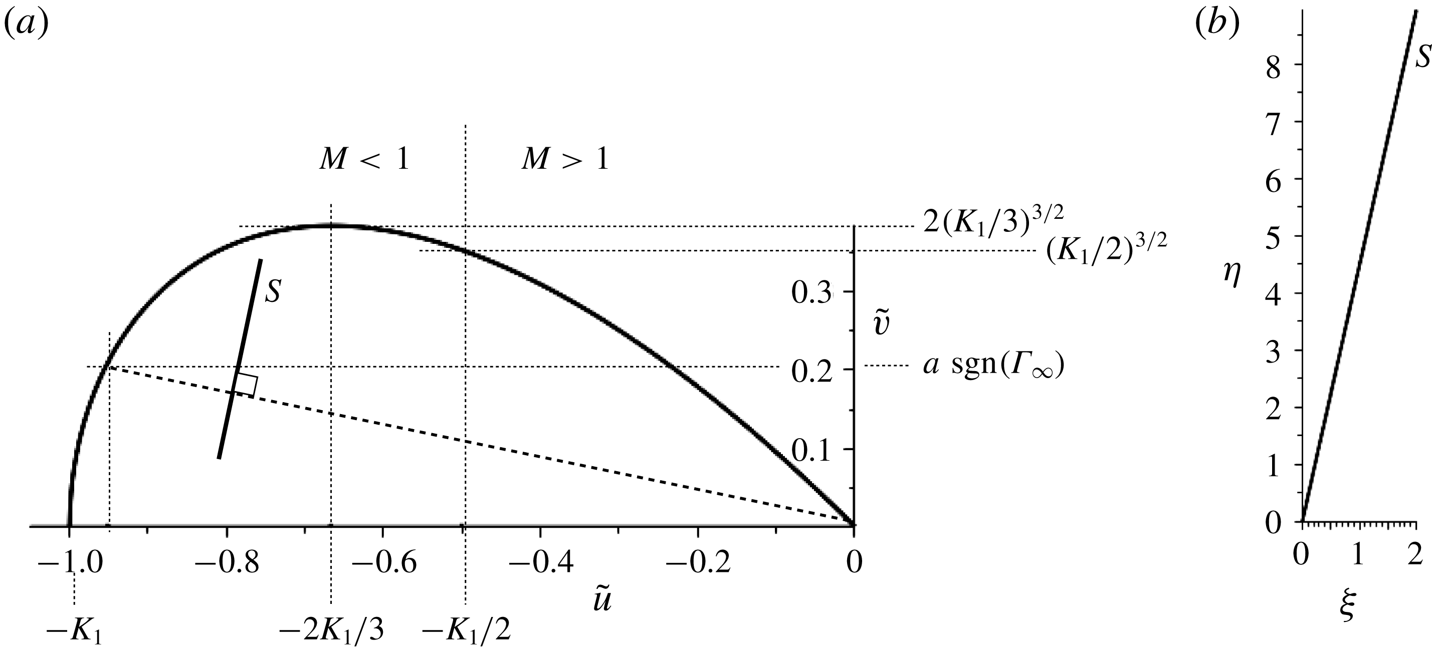
We now consider upstream supersonic flow over an infinite ramp that generates an oblique shock located at the corner of the ramp. The resulting downstream flow deflected through the shock is parallel with the inclined ramp surface. We plot in figure 3(a) the shock polar given by (4.10) for
 $K_{1}=1,K_{2}=0$
and include the construction associated with a jump to a downstream state
 $\tilde{u} =-0.95$
. The line
 $S$
is orthogonal to the shock cord and gives the shock slope in the
 $(\unicode[STIX]{x1D709},\unicode[STIX]{x1D702})$
plane, as shown in figure 3(b). For
 $\unicode[STIX]{x1D6E4}_{\infty }>0$
the corner is concave and the shocks are classical compression shocks – a result readily deduced from (3.8), as then the perturbed density
 $\bar{\unicode[STIX]{x1D70C}}$
is related to
 $\tilde{u}$
by
 $\bar{\unicode[STIX]{x1D70C}}\approx -(\unicode[STIX]{x1D6FF}^{2/3}\tilde{u} )/\unicode[STIX]{x1D6E4}_{\infty }^{1/3}$
. In contrast for
 $\unicode[STIX]{x1D6E4}_{\infty }<0$
the corner is convex and the shock is an expansive shock.
(a) The shock polar for
 $K_{1}>0$
,
 $K_{2}=0$
with the construction of a shock discontinuity. Results are given for
 $K_{1}=1$
and a jump downstream to
 $\tilde{u} =-0.95$
. (b) The corresponding shock represented in the
 $(\unicode[STIX]{x1D709},\unicode[STIX]{x1D702})$
plane is shown with the shock slope given by the line
 $S$
in (a) which is orthogonal to the Rayleigh line (heavy dashed line) in the polar plot.

The construction indicates that for a given flow deflection, i.e. an angle
 $a$
, there are in general two possible states downstream of the shock corresponding to a weak and strong shock. In general, the weak shock connects to supersonic downstream states and the strong shock to subsonic downstream states. The downstream flow becomes subsonic for
 $\tilde{u} <-K_{1}/2$
. For the case of infinitesimal flow deflection we either have the flow limiting to a Mach wave or a normal shock of strength given by a downstream state
 $u_{2}=-K_{1}$
. Maximum flow deflection occurs where the two possible shocks coincide and for
 $|a|>a_{max}$
the configuration involving a shock located at the corner of the ramp cannot be realised. Depending on the sign of
 $\unicode[STIX]{x1D6E4}_{\infty }$
, the corner geometry for maximum deflection is either concave or convex. Flows corresponding to
 $a_{max}$
are approximated by flows where
 $\tilde{v}$
is a maximum, with corresponding deflections
 $$\begin{eqnarray}\displaystyle & \displaystyle a_{max}=2\left({\displaystyle \frac{K_{1}}{3}}\right)^{3/2}~\text{sgn}(\unicode[STIX]{x1D6E4}_{\infty })+O(\unicode[STIX]{x1D6FF}^{1/2}). & \displaystyle\end{eqnarray}$$
Shock solutions describe the transition between two constant states associated with the uniform flow around a sharp corner. Simple waves can also arise when we consider the acceleration of supersonic flows around a concave corner geometry for
 $\unicode[STIX]{x1D6E4}_{\infty }>0$
or the deacceleration of supersonic flows around a convex corner geometry for
 $\unicode[STIX]{x1D6E4}_{\infty }<0$
.
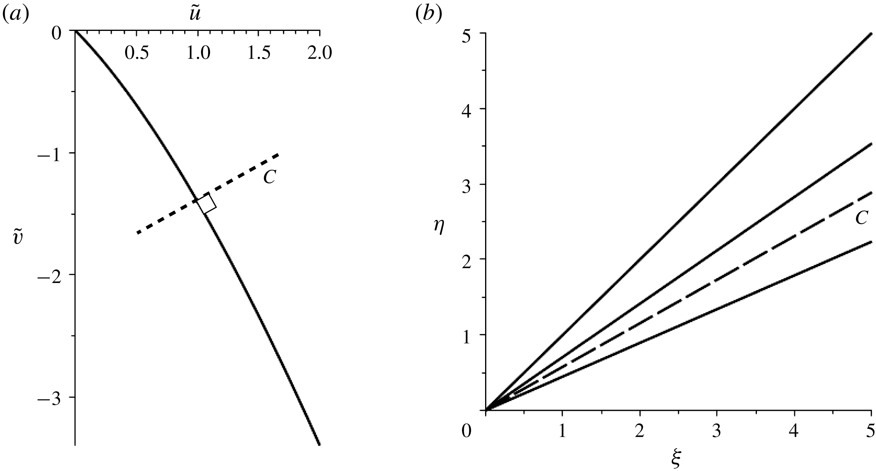
(a) Hodograph characteristic curve for
 $K_{1}>0$
,
 $K_{2}=0$
. Results are displayed for
 $K_{1}=1$
and a transition to the downstream flow
 $\tilde{u} =2$
. (b) The corresponding wavefan in the
 $(\unicode[STIX]{x1D709},\unicode[STIX]{x1D702})$
plane. The characteristic for
 $\tilde{u} =1$
indicated by the dashed line in (b) has slope given by the dashed line
 $C$
in (a) which is orthogonal to the characteristic curve at
 $\tilde{u} =1$
.

For the case
 $K_{1}>0$
,
 $K_{2}=0$
we can construct a centred simple wave located at the corner of the ramp and connecting the constant states
 $\tilde{v}=0$
upstream and
 $\tilde{v}=a\operatorname{sgn}(\unicode[STIX]{x1D6E4}_{\infty })$
downstream. The image of the physical flow lies along a single characteristic in the
 $(\tilde{u} ,\tilde{v})$
hodograph plane given by integrating (4.7) from the upstream state
 $(\tilde{u} =0,\tilde{v}=0)$
to yield
 $$\begin{eqnarray}\displaystyle & \displaystyle \tilde{v}(\tilde{u} )=-{\textstyle \frac{1}{3}}((K_{1}+2\tilde{u} )^{3/2}-{\textstyle \frac{1}{3}}K_{1}^{3/2}). & \displaystyle\end{eqnarray}$$
This characteristic is shown in figure 4(a). Each point on the characteristic in the hodograph plane is the image of a characteristic that generates the wavefan in the physical plane. We plot also in figure 4(b) the flow in the
 $(\unicode[STIX]{x1D709},\unicode[STIX]{x1D702})$
plane and indicate the geometric construction that connects the hodograph and physical plane. For
 $\unicode[STIX]{x1D6E4}_{\infty }>0$
the corner is convex and the wavefan is an expansion fan. In contrast for
 $\unicode[STIX]{x1D6E4}_{\infty }<0$
the corner is concave and the wavefan is a compressive flow. To complete our discussion of the classical case we note that the analysis and figures presented are restricted to a consideration of characteristics and shocks which are inclined downstream. This is consistent with the uniform upstream boundary conditions imposed on the problem.
We now consider flows where
 $\unicode[STIX]{x1D6EC}_{\infty }\neq 0$
i.e.
 $K_{2}\neq 0$
. The distinguishing feature is that the Mach number
 $M$
given by (3.32) and proportional to
 $-\text{d}j/\text{d}\tilde{u}$
now ceases to vary monotonically with
 $\tilde{u}$
. The extremum of
 $M$
occurs for
 $\tilde{u} =1/K_{2}$
and corresponds to an inflection point in the
 $j(\tilde{u} )$
curve. Attempting through isolated shocks or wavefans to construct flows from
 $\tilde{u} =0$
upstream to
 $\tilde{u}$
values downstream that pass through state
 $\tilde{u} =1/K_{2}$
can lead to singularities in the flow. For wavefans the characteristic slopes vary with
 $\sqrt{M-1}$
and the existence of an extremum for
 $M$
leads to the fan turning back on itself if one attempts to increase the strength of the fan beyond this extremum point. This singularity in the structure of the fan limits the strength of an acceptable wavefan. Similarly there is a limitation on shock strengths where the existence of an inflection point for
 $j(\tilde{u} )$
results in a shock strength limited by sonic downstream conditions such that the equality in (3.29) holds and
 $$\begin{eqnarray}\displaystyle & \displaystyle -{\displaystyle \frac{[j]}{[\tilde{u} ]}}=\left.-{\displaystyle \frac{\text{d}j}{\text{d}\tilde{u} }}\right|_{2}, & \displaystyle\end{eqnarray}$$
and gives a downstream state
 $\tilde{u_{2}}=3/2K_{2}$
.
The non-classical features just described arise in flows for which
 $K_{2}\neq 0$
, and generate sonic shocks and compound wavefan/shock structures which have no counterpart in classical shock dynamics. We explore these solutions first of all for the parameter interval
 $-(3/4K_{1})<K_{2}<0$
.
The function
 $-j(u)$
for
 $K_{1}>0$
,
 $-(3/4K_{1})<K_{2}<0$
. The state
 $\tilde{u} =\tilde{u} ^{\ast }$
corresponds to downstream sonic flow conditions (
 $M=1$
) and
 $\tilde{u} _{n}$
represents downstream flows generated by a normal shock.

4.3.2 Case
$K_{1}>0$
,
$-(3/4K_{1})<K_{2}<0$


Inspection of figure 5, where
 $-j(\tilde{u} )$
is plotted, and comparison with figure 2 shows that this case is qualitatively similar to the classical case just discussed for negative values of
 $\tilde{u}$
in the range
 $\tilde{u} _{n}\leqslant \tilde{u} \leqslant 0$
and all positive
 $\tilde{u}$
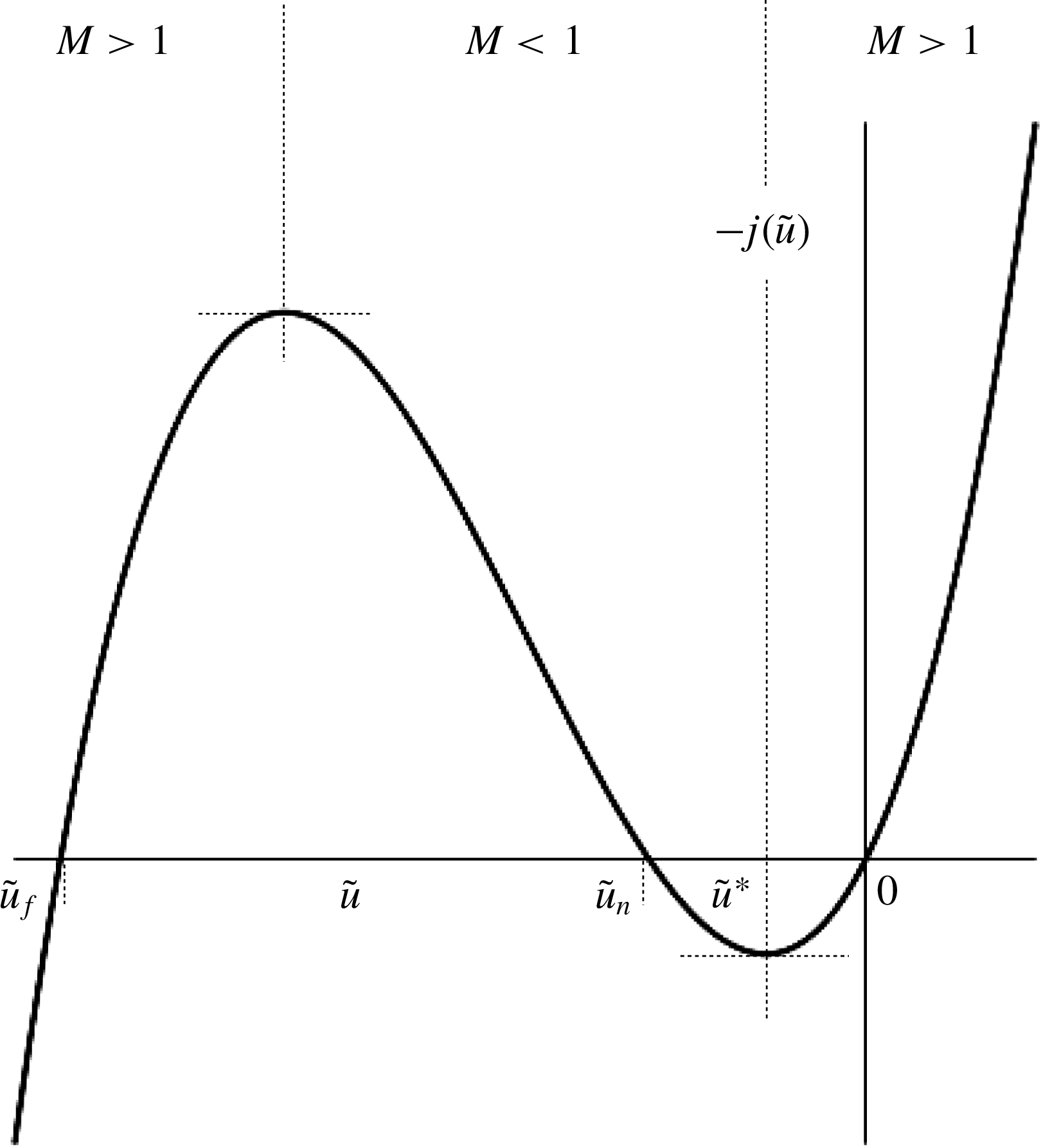
values. It would appear also from figure 5 that an additional shock solution branch exists for
 $\tilde{u} \leqslant \tilde{u} _{f}$
, where
 $-j(\tilde{u} )$
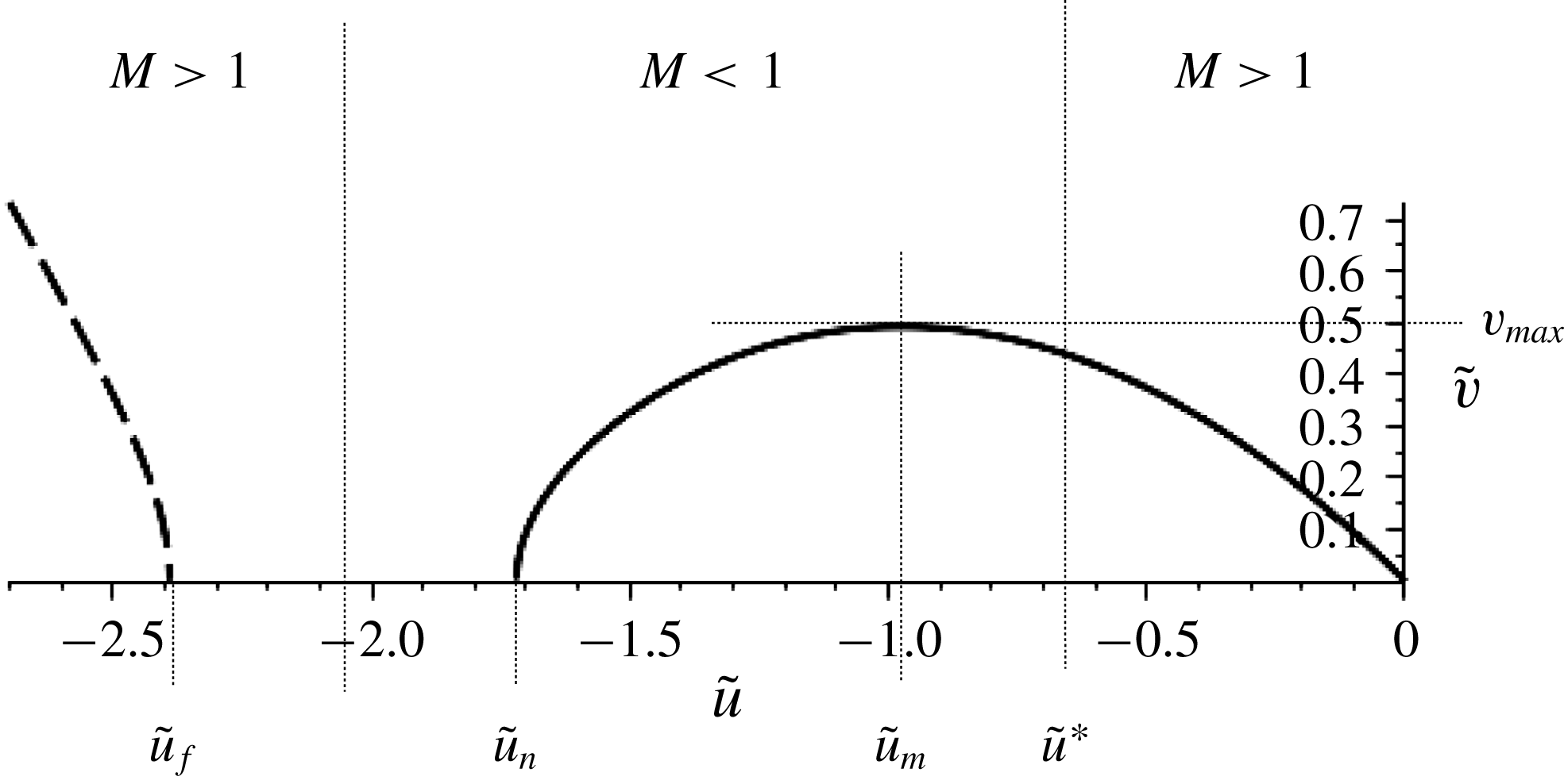
is negative. The shock polar given by (4.10) is plotted in figure 6 (for the representative case
 $K_{1}=1.0,K_{2}=-0.73$
). An additional isolated branch of the polar plot exists for values of
 $\tilde{u} \leqslant \tilde{u} _{f}$
(indicated by the dashed curve); this branch, however, corresponds to downstream states (and hence corner geometries) involving discontinuities which are too strong and so violate the shock inequalities (3.29). Hence this branch describes transitions that are unrealisable through a steady state shock. For downstream states
 $\tilde{u} <0$
in the interval
 $$\begin{eqnarray}\displaystyle & \displaystyle \tilde{u} _{n}={\displaystyle \frac{3}{2K_{2}}}\left(1-\sqrt{1+{\displaystyle \frac{4}{3}}K_{1}K_{2}}\right)\leqslant \tilde{u} \leqslant 0 & \displaystyle\end{eqnarray}$$
shocks do arise and the flow generated can be described by a single attached shock. Within this interval the downstream states become subsonic for
 $$\begin{eqnarray}\displaystyle & \displaystyle \tilde{u} ={\displaystyle \frac{1}{K_{2}}}(1-\sqrt{1+K_{1}K_{2}})=\tilde{u} ^{\ast }, & \displaystyle\end{eqnarray}$$
where
 $\tilde{u} ^{\ast }$
satisfies
 $-j(\tilde{u^{\ast }})/\text{d}\tilde{u} =0$
, as shown in figure 5. Decreasing downstream values of
 $\tilde{u} <\tilde{u} ^{\ast }$
remain subsonic until
 $\tilde{u} =\tilde{u} _{n}$
, at which point the shock is normal to the incoming flow with zero flow deflection resulting. Maximum flow deflection occurs, as shown in figure 6, for
 $\tilde{v}=\tilde{v}_{max}$
, corresponding to a jump to the downstream state
 $$\begin{eqnarray}\displaystyle & \displaystyle \tilde{u} ={\displaystyle \frac{9}{8K_{2}}}(1-\sqrt{1+{\displaystyle \frac{32}{27}}K_{1}K_{2}})=\tilde{u} _{m}. & \displaystyle\end{eqnarray}$$
Shock solutions just described are similar to those for the classical
 $K_{2}=0$
case. This similarity extends to centred wavefan solutions. Such solutions are represented in the hodograph plane by the characteristic curve which is the integral of (4.7). This integral is easily calculated but reproduces similar quantitative results to those displayed in figure 4 for case
 $K_{2}=0$
.
Shock polars for
 $K_{1}=1$
,
 $K_{2}=-0.73$
. Dashed curve denotes a possible additional potential strong shock branch that however violates the shock inequalities.

4.3.3 Case
$K_{1}>0$
,
$-(1/K_{1})<K_{2}<-(3/4K_{1})$


The previous case describes fluids with thermodynamic properties such that the second nonlinear term in (3.17) identified with the parameter
 $\unicode[STIX]{x1D6EC}_{\infty }$
is sufficiently weak, leading to flows qualitatively similar to the classical (
 $\unicode[STIX]{x1D6EC}_{\infty }=0$
) case. With decreasing values of
 $K_{2}$
(and so for larger negative values of
 $\unicode[STIX]{x1D6EC}_{\infty }$
), such that
 $K_{2}$
now lies in the interval
 $-(1/K_{1})<K_{2}<-(3/4K_{1})$
, the shock structure for transitions to negative values of
 $\tilde{u}$
begins to exhibit certain novel features. These can be deduced from the plot for
 $-j(\tilde{u} )$
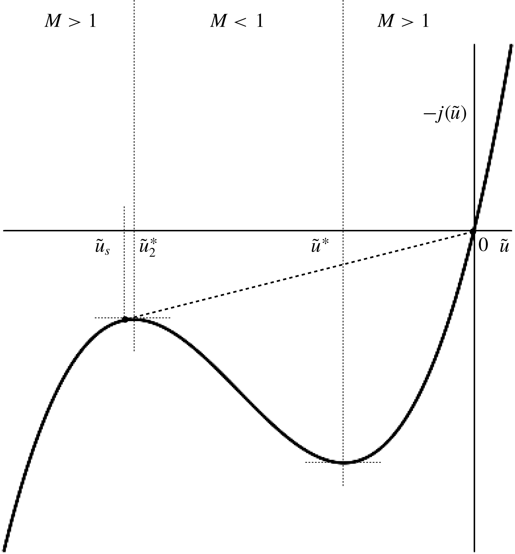
shown in figure 7. The second turning point for
 $-j(\tilde{u} )$
located at
 $\tilde{u} _{2}^{\ast }$
now occurs for negative values of
 $-j(\tilde{u} )$
and shock jumps to
 $\tilde{u} _{2}^{\ast }$
are possible. Strong normal shocks associated with
 $-j(\tilde{u} )=0$
are now not possible and instead the shock of maximum strength is given by the downstream state
 $\tilde{u} _{s}=3/2K_{2}$
, where
 $$\begin{eqnarray}\displaystyle & \displaystyle \left.-{\displaystyle \frac{\text{d}j}{\text{d}\tilde{u} }}\right|_{\tilde{u} _{s}}=-{\displaystyle \frac{[j]}{[\tilde{u} ]}}. & \displaystyle\end{eqnarray}$$
This is indicated in figure 7, where the slope of the straight line connecting the upstream state
 $\tilde{u} =0$
to the downstream state
 $\tilde{u}$
is tangent to
 $-j(\tilde{u} )$
at
 $\tilde{u} =\tilde{u} _{s}$
. A construction similar to this arises in nonlinear progressive waves (see Kluwick Reference Kluwick and Kluwick1991). As for progressive waves it should also be possible to connect to downstream states
 $\tilde{u} <\tilde{u} _{s}$
, where
 $\tilde{u}$
is now supersonic – not through shock transitions but through compound sonic-shock/wavefan structures.
The function
 $-j(u)$
for
 $K_{1}>0$
,
 $-(1/K_{1})<K_{2}<-(3/4K_{1})$
. The line (dashed) represents a shock with sonic downstream state
 $\tilde{u} _{s}$
connecting to state
 $\tilde{u} =0$
upstream.

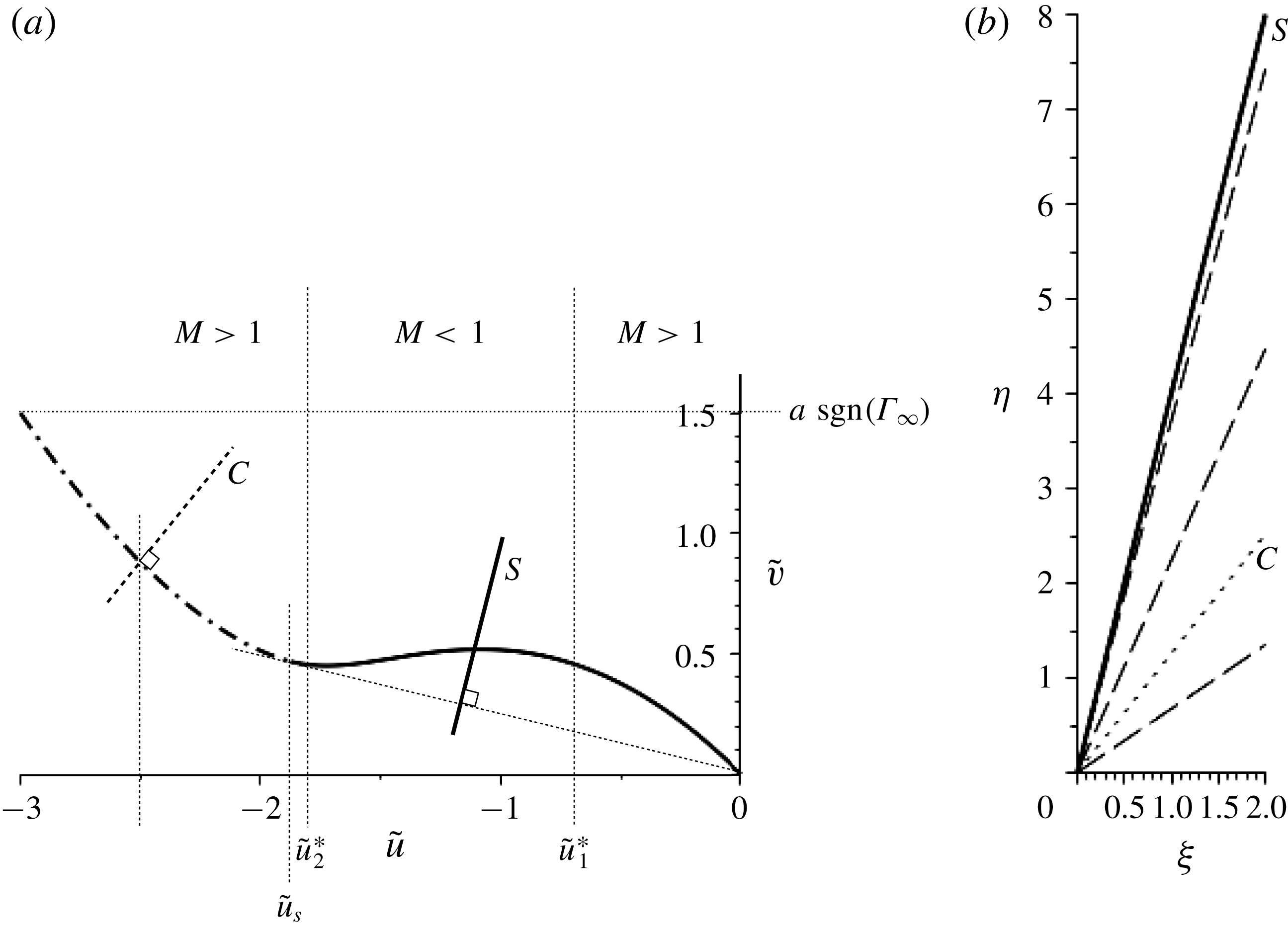
The flow scenarios described above are represented in the hodograph plane shown in figure 8(a) for the particular case
 $K_{1}=1$
,
 $K_{2}=-0.8$
. From the upstream state
 $\tilde{u} =0$
we consider decreasing downstream values
 $\tilde{u}$
until the expected transition from supersonic to a subsonic downstream state occurs at
 $\tilde{u} _{1}^{\ast }$
. Continuing to decrease
 $\tilde{u}$
the flow deflection (measured by
 $\tilde{v}$
) increases to a maximum before decreasing again. Before a normal shock becomes possible, as already discussed, the downstream flows turn supersonic at
 $\tilde{u} _{2}^{\ast }$
. Further decreasing
 $\tilde{u}$
downstream results in the flow deflection increasing until eventually a limiting shock of maximum strength is reached corresponding to sonic conditions holding for the downstream state
 $\tilde{u} =\tilde{u} _{s}=3/2K_{2}$
.
(a) The shock polar and characteristic for
 $K_{1}>0$
and
 $-(1/K_{2})<K_{2}<-(3/4K_{1})$
with the construction of a sonic-shock/wavefan flow transition. Results are given for
 $K_{1}=1$
and
 $K_{2}=-0.8$
and a downstream state
 $\tilde{u} =-3.0$
. (b) The corresponding sonic shock/wavefan in the
 $(\unicode[STIX]{x1D709},\unicode[STIX]{x1D702})$
plane is shown. The sonic shock is the line labelled
 $S$
, which is orthogonal to the Rayleigh line (light dashed) in the polar plot in (a). The physical characteristics in (b) are orthogonal to the hodograph characteristic (dot-dashed line) in (a), as indicated by the particular construction for
 $\tilde{u} =-2.5$
(lines labelled
 $C$
).

The shock polar terminates at
 $\tilde{u} =\tilde{u} _{s}$
; however, flows with downstream states
 $\tilde{u} <\tilde{u} _{s}$
are still possible, but now only through compound sonic shock – attached wavefan structures. The attached wavefan is given by the integral curve of (4.7).
In figure 8(b) we show the sonic-shock/wavefan construction in the physical
 $(\unicode[STIX]{x1D709},\unicode[STIX]{x1D702})$
plane which describes a transition to a downstream state
 $\tilde{u} =-3.0$
.
Transitions to positive downstream states are described by a centred wavefan similar to the classical case and the generated flow exhibits no new behaviour.
Two novel features of the flows generated here are important to note. Firstly, (aside from the assumptions leading to the model equations) there is no maximum deflection angle. Secondly, there are values of the deflection angle for which there are three possible flow configurations – weak shocks, strong shocks and a compound sonic-shock/wavefan structure.
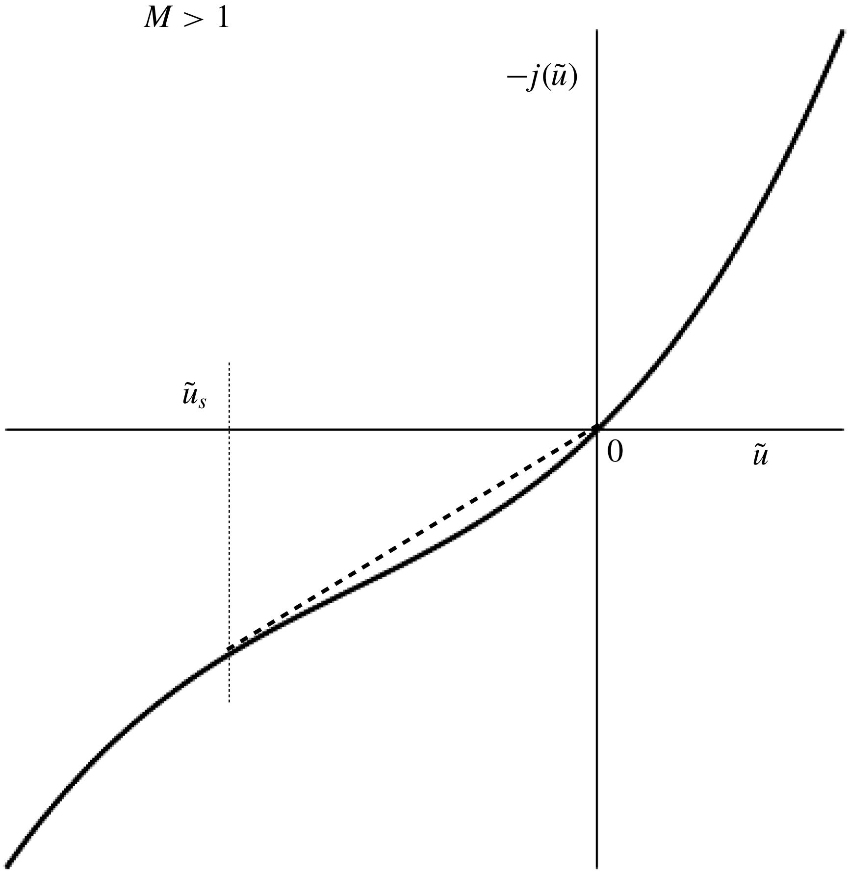
The function
 $-j(u)$
for
 $K_{1}>0$
,
 $K_{2}<-1/K_{1}$
with a sonic shock at
 $\tilde{u} _{s}$
where the dashed line connecting to state
 $\tilde{u} =0$
upstream is tangent to
 $-j(\tilde{u} )$
at
 $\tilde{u} _{s}$
.

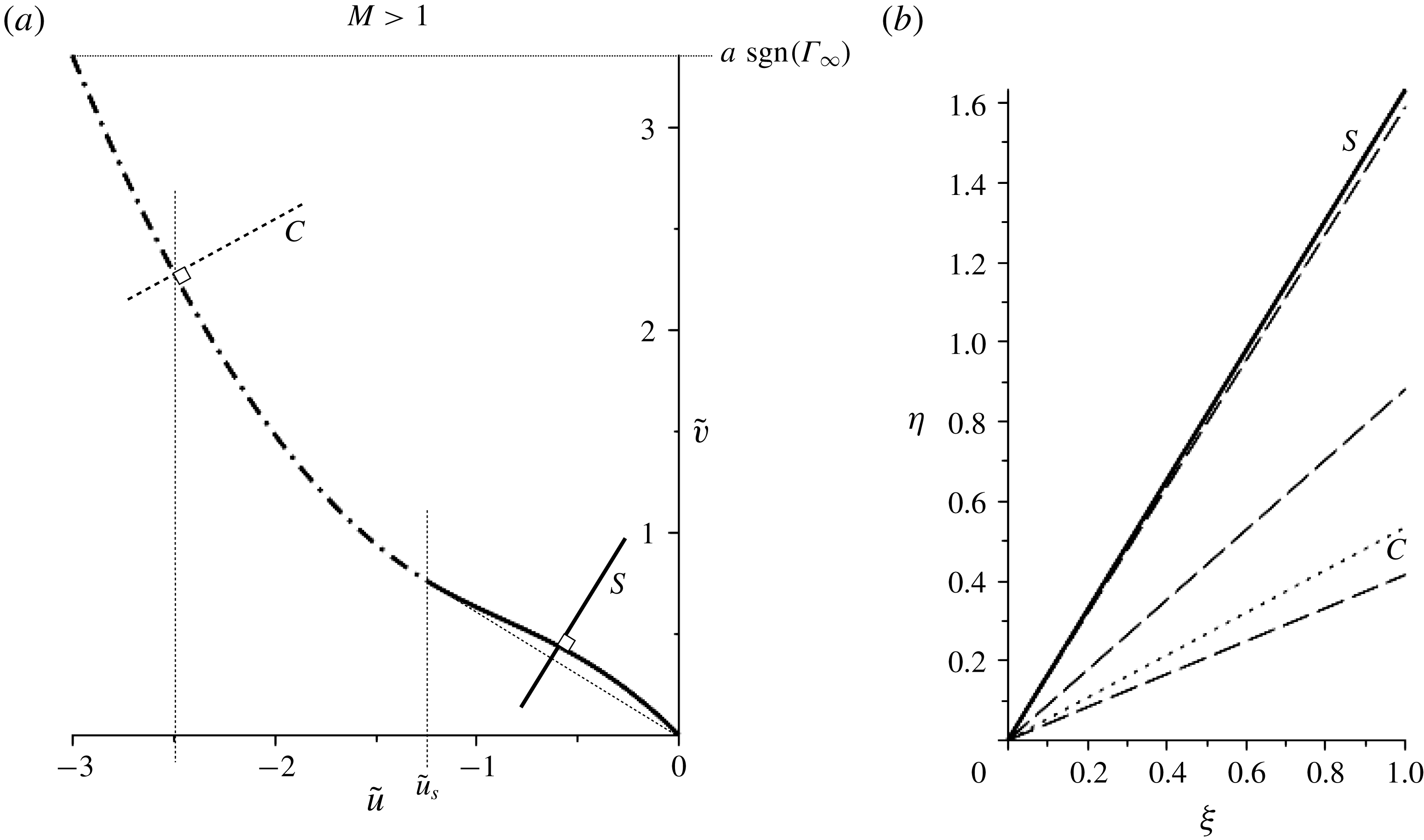
(a) The shock polar and characteristic for
 $K_{1}>0$
and
 $K_{2}<-1/K_{1}$
with the construction of a sonic-shock/wavefan flow transition. Results are given for
 $K_{1}=1$
and
 $K_{2}=-1.2$
and a downstream state
 $\tilde{u} =-3.0$
. (b) The corresponding sonic shock/wavefan in the
 $(\unicode[STIX]{x1D709},\unicode[STIX]{x1D702})$
plane is shown. The sonic shock is the line labelled
 $S$
, which is orthogonal to the sonic-shock chord in the polar plot in (a). The physical characteristics in (b) are orthogonal to the hodograph characteristic in (a), as indicated by the particular construction for
 $\tilde{u} =-2.5$
(lines labelled
 $C$
).

4.3.4 Case
$K_{1}>0$
,
$K_{2}<-1/K_{1}$


If we continue to decrease the parameter
 $K_{2}$
then eventually with
 $K_{2}<-1/K_{1}$
we have the
 $-j(\tilde{u} )$
plot shown in figure 9. The slope of
 $-j(\tilde{u} )$
is positive for all
 $\tilde{u}$
, and hence there is no subsonic downstream flows. Again as in the previous case shocks are possible for downstream states in the interval
 $\tilde{u} _{s}<\tilde{u} <0$
, where
 $\tilde{u} _{s}$
satisfies (4.24). Sonic conditions are generated downstream for
 $\tilde{u} =\tilde{u} _{s}$
, as indicated in figure 9, and as in the previous case then the transition to larger negative values of
 $\tilde{u}$
is accomplished through a compound sonic-shock/fan structure. For positive values of
 $\tilde{u}$
a centred wavefan similar to the classical case is generated. In figure 10(a) we show the shock, shock–fan representations in the hodograph plane. The maximum flow deflection generated by an isolated shock now occurs at the sonic shock. In figure 10(b) we show the sonic-shock/wavefan construction in the physical
 $(\unicode[STIX]{x1D709},\unicode[STIX]{x1D702})$
plane describing a transition to a downstream state
 $\tilde{u} =-3.0$
.
4.3.5 Summary for
$K_{1}>0$
,
$K_{2}<0$


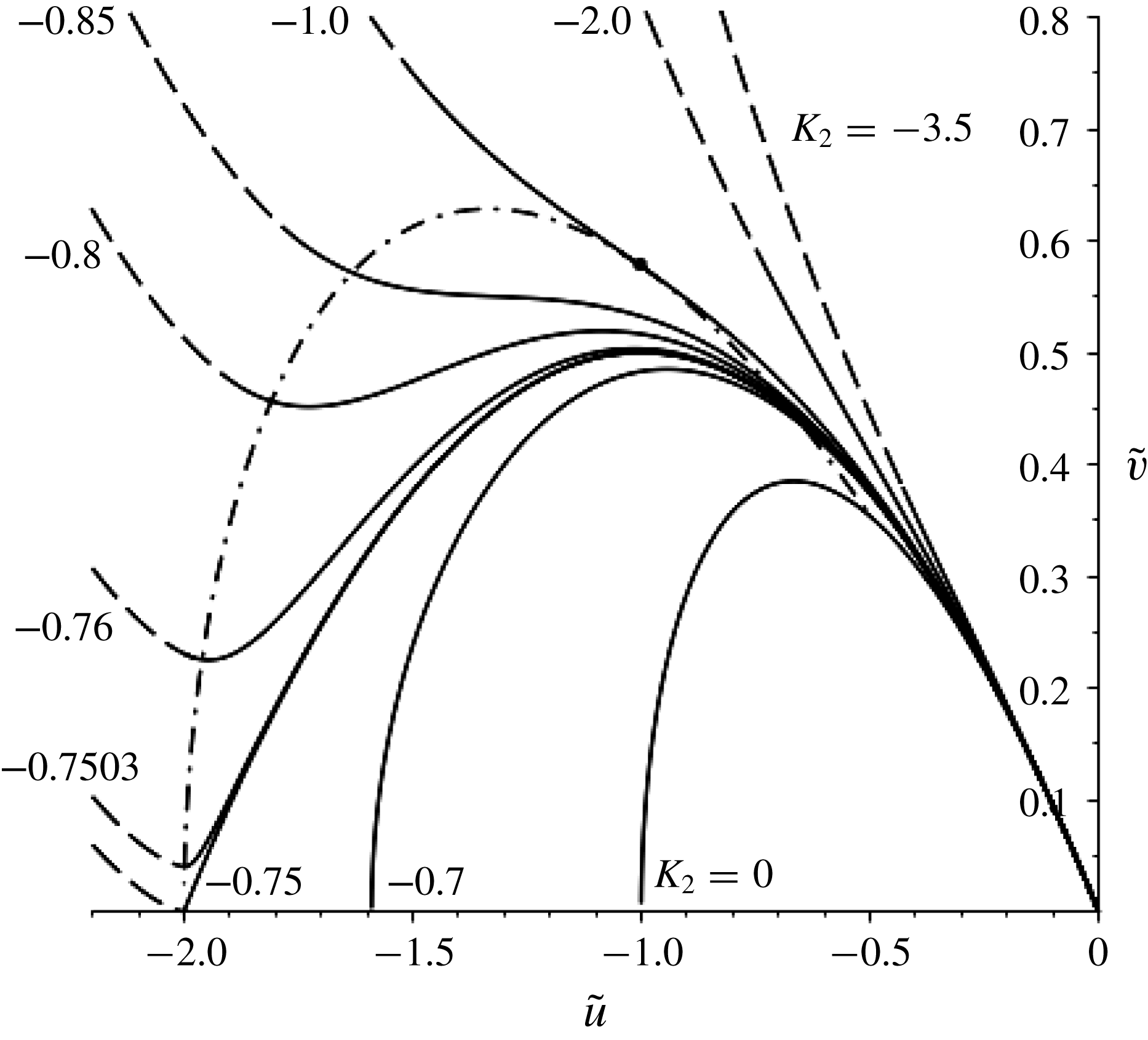
The results of the various flow scenarios for
 $K_{1}>0$
,
 $K_{2}<0$
are summarised in figure 11. Results are for the particular representative case
 $K_{1}=1$
. As already discussed for gases with
 $-(3/4K_{1})<K_{2}<0$
the shock solution is similar to the classical
 $K_{2}=0$
case. For
 $-(1/K_{1})<K_{2}<-(3/4K_{2})$
the classical solutions involving a weak and strong shock for a given wedge angle are now enriched through a possible third flow transition by means of a sonic-shock/wavefan construction. Furthermore, for small wedge angles the flow is unique, with only weak shocks being possible. Finally, for
 $K_{2}<-1/K_{1}$
the flow is unique for all wedge angles and consists of either a classical shock or a sonic-shock/fan transition with supersonic downstream states.
Permissible downstream states represented in the
 $(\tilde{u} ,\tilde{v})$
hodograph plane connected by either a shock or a compound sonic shock–fan to upstream state
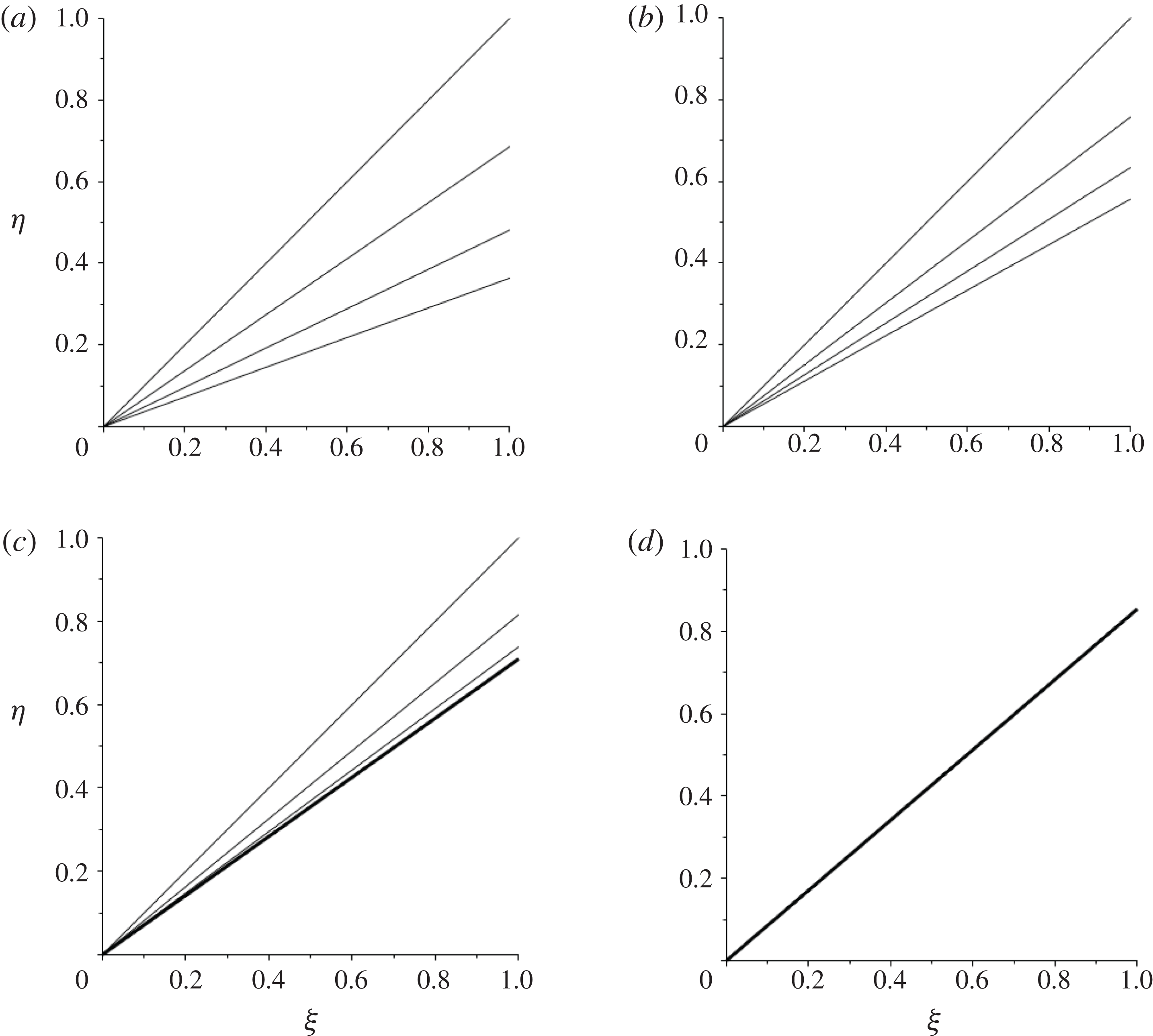
 $\tilde{u} =0,\tilde{v}=0$
for
 $K_{1}=1$
and varying
 $K_{2}\leqslant 0$
. Shock polars are plotted as solid lines, wavefans are plotted as dashed lines, and sonic points lie on the dash-dotted curve.

4.3.6 Case
$K_{1}>0$
,
$K_{2}>0$


 $0<K_{2}<3/K_{1}$
. It remains now to consider positive values of the parameter
 $K_{2}$
describing flow for fluids with positive
 $\unicode[STIX]{x1D6EC}_{\infty }$
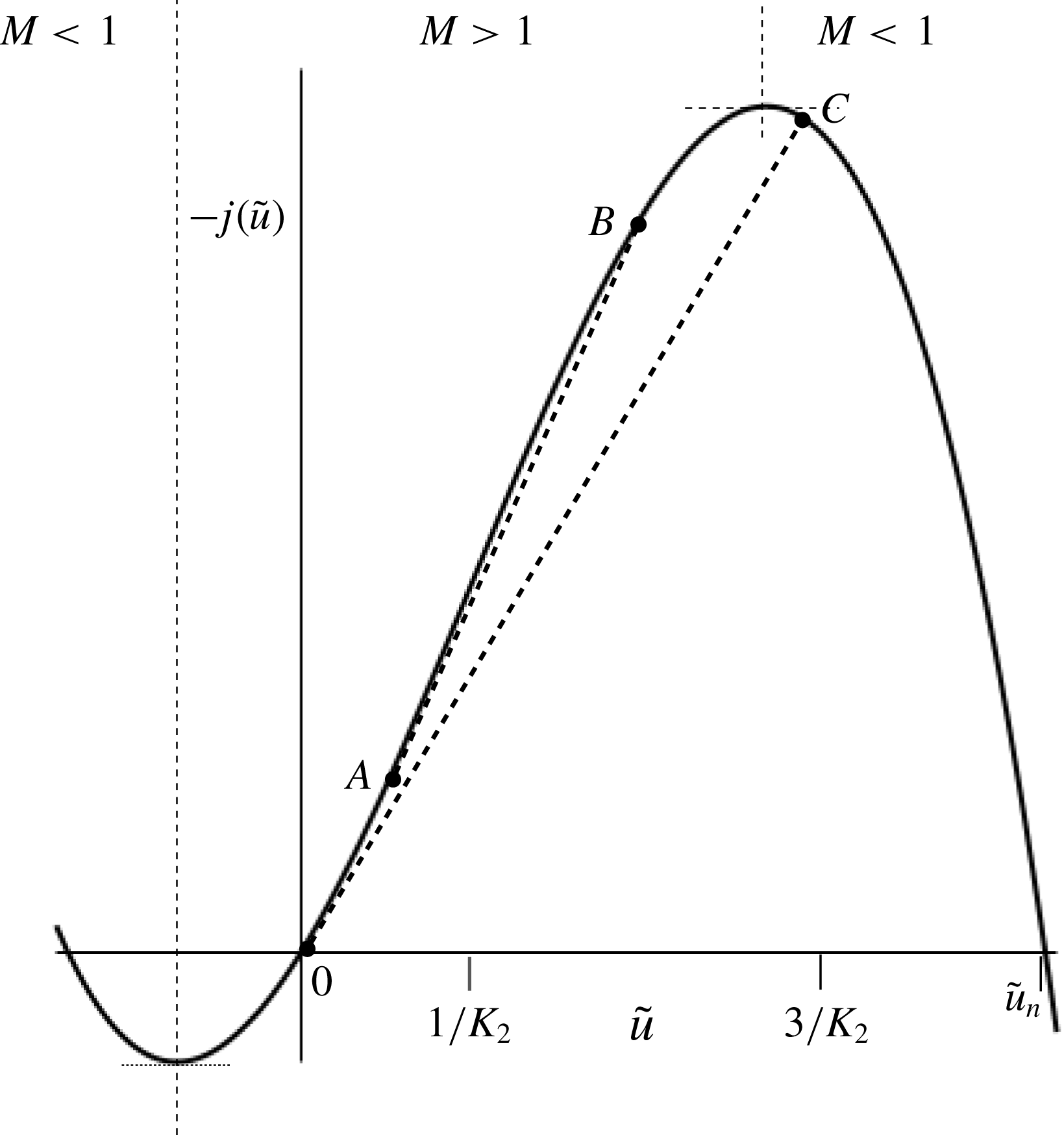
. We first consider the case
 $0<K_{2}<3/K_{1}$
and the appropriate plot of
 $-j(\tilde{u} )$
is shown in figure 12. For negative downstream values of
 $\tilde{u}$
the flow is similar to the classical
 $K_{2}=0$
case and one expects classical shock dynamic behaviour. A connection to positive downstream states is also possible as in the classical case through an expansion wavefan construction. However, this is only possible for values of
 $\tilde{u}$
in the interval
 $(0,1/K_{2})$
. The slope of characteristics in the wavefan is given by (4.16), with a turning point occurring when
 $-(\text{d}^{2}j(\tilde{u} ))/\text{d}\tilde{u} ^{2}=0$
, i.e. at
 $\tilde{u} =1/K_{2}$
. This limits the strength of the wavefan and is in contrast to the classical case where there is no such limit. It is still possible to connect to downstream states
 $\tilde{u} >1/K_{2}$
, but only through compound fan–sonic-shock structures – a construction that is analogous to the one-dimensional evolution problem considered by Cramer & Kluwick (Reference Cramer and Kluwick1984). The sonic shock is attached to the wavefan, and at the point of attachment the shock slope is equal to the slope of the terminating characteristic of the wavefan in the physical domain. This is indicated in figure 12, with the sonic shock represented as the straight line
 $AB$
connecting state
 $B$
downstream to state
 $A$
such that the line
 $AB$
is tangential to
 $-j(\tilde{u} )$
at point
 $A$
. This sonic-shock condition at
 $A$
is given by
 $$\begin{eqnarray}\displaystyle & \displaystyle \left.-{\displaystyle \frac{\text{d}j}{\text{d}\tilde{u} }}\right|_{A}=-{\displaystyle \frac{[j]}{[\tilde{u} ]}}, & \displaystyle\end{eqnarray}$$
which uniquely determines the downstream state
 $$\begin{eqnarray}\displaystyle & \displaystyle \tilde{u} _{B}={\displaystyle \frac{3}{K_{2}}}-2\tilde{u} _{A}. & \displaystyle\end{eqnarray}$$
As we continue to increase
 $\tilde{u}$
downstream the shock remains sonic and its strength increases while the wavefan strength diminishes. Eventually when
 $\tilde{u} _{B}=3/K_{2}$
we have simply a sonic shock connecting the downstream state
 $\tilde{u} _{B}$
to the upstream state
 $\tilde{u} =0$
, as indicated also in figure 12, where this downstream state is identified with the point
 $C$
. Increasing
 $\tilde{u}$
still further we have strong (but non-sonic) expansion shock solutions generated until the downstream state
 $$\begin{eqnarray}\displaystyle & \displaystyle \tilde{u} _{n}={\displaystyle \frac{3}{2K_{2}}}\left(1+\sqrt{1+{\displaystyle \frac{4}{3}}K_{1}K_{2}}\right), & \displaystyle\end{eqnarray}$$
where the resulting shock is normal to the flow.
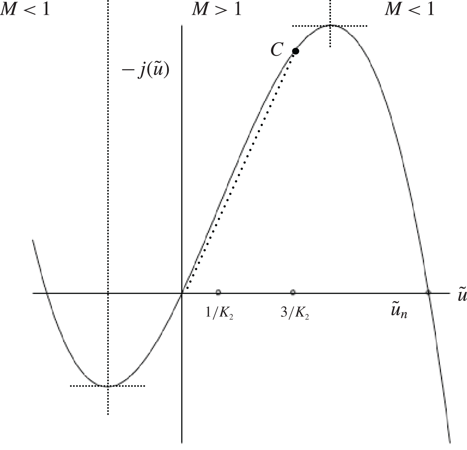
The function
 $-j(u)$
for
 $K_{1}>0$
,
 $0<K_{2}<3/K_{1}$
. The dashed line
 $AB$
corresponds to shocks which are sonic at point
 $A$
. The dashed curve terminating at
 $C$
is a shock which connects to
 $\tilde{u} =0$
upstream where sonic conditions hold.

Downstream states are subsonic for
 $\tilde{u} >1/K_{2}(1+\sqrt{1+K_{1}K_{2}})$
with
 $-\text{d}j/\text{d}u<0$
and it is easily determined that for
 $0<K_{2}<3/K_{1}$
(as seen in figure 12) sonic jumps have supersonic downstream states for small
 $\tilde{u}$
but with increasing
 $\tilde{u}$
involve transitions to subsonic states.
Fan, compound shock–fan and single shock structures for
 $K_{1}>0$
and
 $0<K_{2}<3/2K_{1}$
. Results are depicted for
 $K_{2}=1,K_{1}=1$
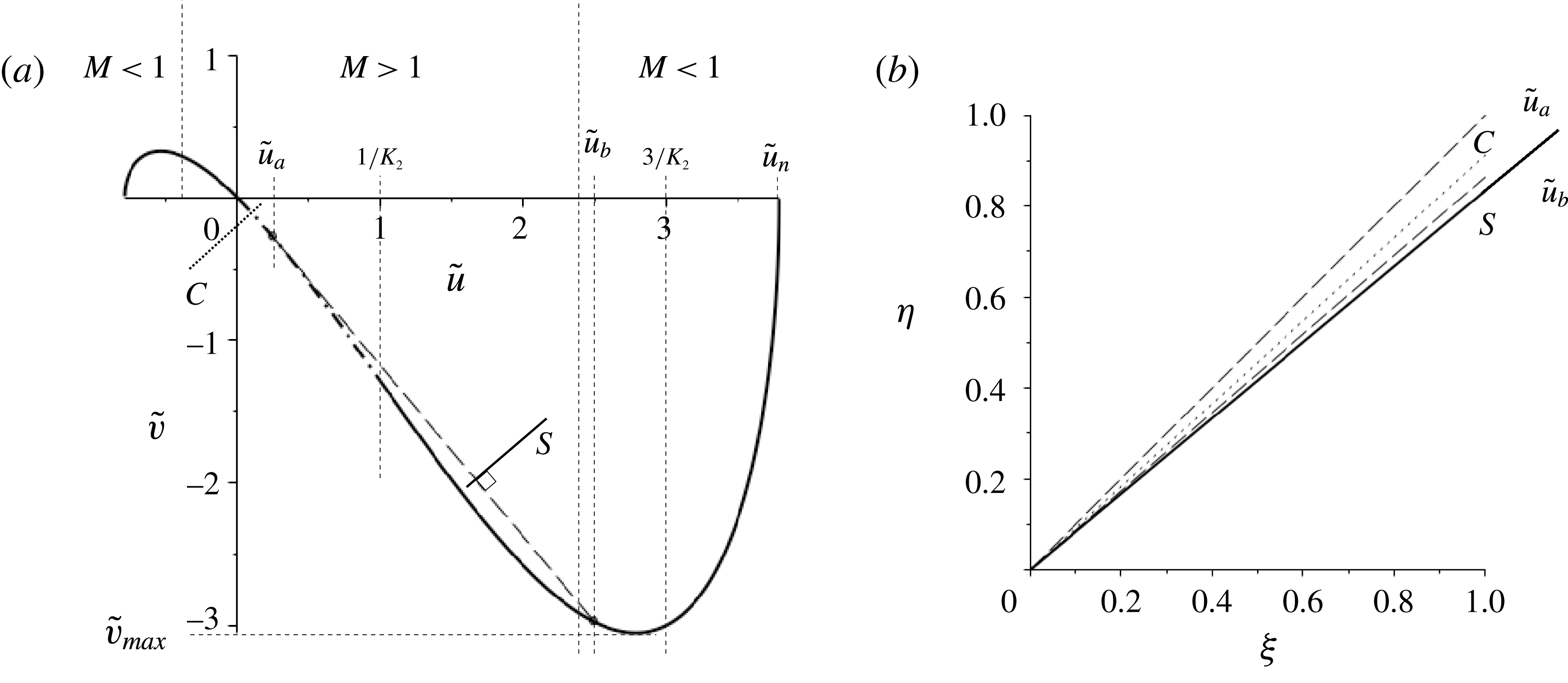
. (a) Hodograph plane representation. Dot-dashed line is the characteristic curve, solid line is the shock polar and the dashed line is the Rayleigh line. An expansion fan exists for downstream states
 $0<\tilde{u} <1/K_{2}$
. Transitions to downstream states
 $1/K_{2}<\tilde{u} <3/K_{2}$
involve fan/sonic-shock flows. Shown is the construction representing a wavefan expansion to
 $\tilde{u} _{a}$
followed by a sonic jump to downstream state
 $\tilde{u} _{b}$
. Downstream states
 $3/K_{2}<\tilde{u} <\tilde{u} _{n}$
are reached by classical shock jumps. (b) The resulting flow geometry in the (
 $\unicode[STIX]{x1D709},\unicode[STIX]{x1D702}$
) plane for the expansion fan/sonic-shock construction leading to a downstream state
 $\tilde{u} =2.5$
. The sonic shock, the line labelled
 $S$
is orthogonal to the shock chord in (a). The characteristics are orthogonal to the hodograph characteristic in (a), as indicated by the particular construction for
 $\tilde{u} =0.1$
(lines labelled
 $C$
). Dashed lines are wavefronts and solid line is a sonic shock.

The flow scenarios described above can be represented in the
 $(\tilde{u} ,\tilde{v})$
hodograph plane, as shown in figure 13(a) for the particular case
 $K_{2}=1,K_{1}=1$
. As already observed, shock solutions exist which lead to a reduction of the velocity
 $\tilde{u}$
and give qualitatively similar results to those observed in perfect gases. These shocks are not included here. In contrast to the classical case, however, an additional branch of the shock polar now exists for
 $\tilde{u} >0$
, and this branch, isolated from the upstream state
 $\tilde{u} =0$
, connects with the characteristic describing accelerated flows. Increasing values of the downstream velocity then causes a transition from a centred wavefan to a wavefan terminated by a sonic rarefaction shock, and finally to a single rarefaction shock. This transition is associated with a non-monotonic variation of the wedge angle parameter
 $a$
, with the maximum deflection of the upstream flow associated with a fan/sonic-shock transition. In figure 13(b) we show the resulting flow geometry in the (
 $\unicode[STIX]{x1D709},\unicode[STIX]{x1D702}$
) plane for the expansion fan/sonic-shock construction leading to a downstream state
 $\tilde{u} =2.5$
. We can also distinguish two subcases: firstly: flows for which
 $0<K_{2}<3/2K_{1}$
, illustrated by figure 13 and identified by the maximum deflection of the upstream flow being generated by a fan/sonic-shock transitions. Then, secondly, flows for
 $(3/2K_{1})<K_{2}<(3/K_{1})$
, where the maximum deflection is instead associated with a classical non-sonic jump. In figure 14 the sonic jump connecting upstream state
 $\tilde{u} =0$
to the downstream state
 $\tilde{u} =3/K_{2}$
is shown as occurring before
 $\tilde{v}_{max}$
is reached.
 $K_{1}>0$
,
 $3/K_{1}<K_{2}$
. Finally we consider the case where with increasing
 $K_{2}$
we have
 $K_{2}>3/K_{1}$
. The plot of
 $-j(\tilde{u} )$
is shown in figure 15 and is similar to that for
 $0<K_{2}<3/K_{1}$
. The key difference is that sonic shocks connect now only to supersonic states downstream. Point
 $C$
corresponds to the maximum strength sonic shock with downstream supersonic flow
 $\tilde{u} =3/K_{2}$
which connects to the upstream state
 $\tilde{u} =0$
.
(a) Hodograph plot for
 $K_{1}>0$
and
 $(3/2K_{1})<K_{2}<(3/K_{1})$
. Results are depicted for
 $K_{2}=1,K_{1}=2$
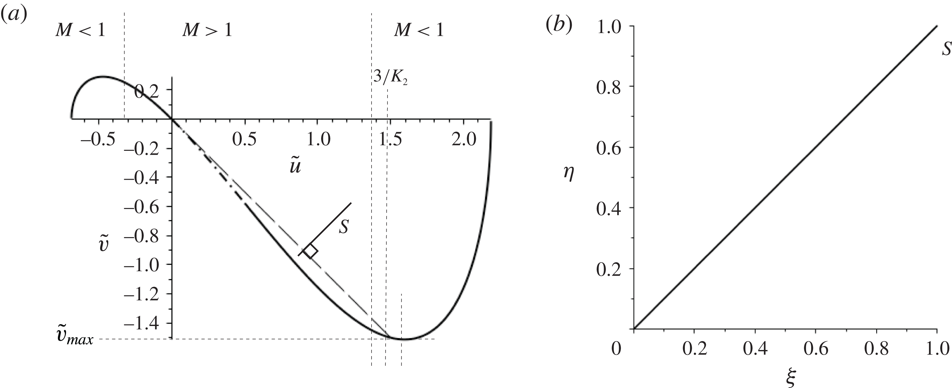
. The construction of a sonic shock is shown in (a) with the shock discontinuity plotted in the (
 $\unicode[STIX]{x1D709},\unicode[STIX]{x1D702}$
) plane in (b). The shock labelled
 $S$
is orthogonal to the shock chord in (a). Maximum deflection is generated by a classical shock. Dashed-dot line is the characteristic, solid line is the shock polar and dashed line is the Rayleigh line.

The function
 $-j(u)$
for
 $K_{1}>0$
,
 $3/K_{1}<K_{2}$
with the dashed line representing a downstream state
 $\tilde{u} =3/K_{2}$
connecting through a shock to
 $\tilde{u} =0$
upstream where sonic conditions hold.

5 Conclusions
Supersonic small-disturbance flow over a ramp or around a corner is a fundamental problem in compressible fluid dynamics. In the case of classical gas dynamics the flows are easily described in terms of compressive shocks and expansion fans (see Cole & Cook Reference Cole and Cook1986). In the context of BZT fluids and so-called mixed nonlinearity the flows are more complex, involving not only expansion shocks but also sonic shocks and shock/fan composite flows. Besides the particular challenge of understanding the flow scenarios for this fundamental problem there is the more general motivation: namely, that the study of 2D steady supersonic flows provides a promising alternative to 1D unsteady flows. This is directed at the experimental clarification of the long-standing question: ‘do rarefaction shocks exist in the dense gas region of so-called BZT fluids having moderate/high molecular complexity?’ A confirming result is predicted clearly by the theory presented in this paper as also in previous extant results (see, for example, Cramer & Tarkenton Reference Cramer and Tarkenton1992). Indeed experimental set-ups for this type of flows are presently in the stage of planning or even construction at various institutions, including the Politecnico di Milano and the University of Delft. These massive efforts are devoted not only to addressing fundamental questions such as that above but also to answer questions relevant to future technological developments, including, for example, energy conversion processes such as organic rankine cycles (ORCs). Of particular relevance to the design and interpretation of wind tunnel experiments and flow behaviour in the entry region of cascades, the results obtained and discussed in § 4 can provide input data for the investigation of the problem of how waves generated by a ramp/wedge are reflected from an opposing solid wall. Here the transition from regular to irregular reflection is of major concern, and for the case of perfect gases has received considerable attention (see, for example, Ben-Dor Reference Ben-Dor2007). Extensions to dense gas flows are definitely required.
Asymptotic analysis predicts that the error associated with perturbation solutions will be of the order of the first neglected term in the expansions, i.e.
 $O(\bar{\unicode[STIX]{x1D70C}}^{2})$
in the case investigated. This has been found consistent with studies of classical transonic flows and there is no obvious reason why it should be different for the type of flows considered here, but numerical calculations might be helpful to clarify this point. In this connection the following comments seem appropriate. Numerical calculations require the choice of specific equations of state. However, even the most advanced equation of state applied to date involve uncertainties concerning, among others, the extent of the region of negative
 $\unicode[STIX]{x1D6E4}$
in the
 $p,1/\unicode[STIX]{x1D70C}$
diagram. For example, the widely used van der Waals and the Martin Hou equations of state are known to overpredict the effects of negative
 $\unicode[STIX]{x1D6E4}$
. Obviously, these deficiencies limit the usefulness of numerical results. In contrast, the predictions of the present small-disturbance approach are largely independent of such detailed knowledge as the only input data are the values of
 $\unicode[STIX]{x1D6E4}$
and
 $\unicode[STIX]{x1D6EC}$
in the unperturbed state. It is therefore felt that analytical and numerical efforts are somewhat complementary in contributing to a better understanding of dense gas flows.
The present paper focusses then on the canonical problem of supersonic ramp flow, which can be realised experimentally with some ease and which has the advantage that the complete theoretical picture follows from the consideration of two basic building blocks – straight oblique shocks and centred wavefans. Asymptotic analysis in the limit of small ramp angles allows for significant analytical progress. Most important it is found that the flow properties are fully determined by a quantity
 $a$
which specifies the ramp angle and two similarity parameters
 $K_{1},K_{2}$
. Here
 $K_{1}$
is the transonic similarity parameter known from the theory of perfect gases. In addition,
 $K_{2}$
accounts for non-classical effects resulting from the requirement that the unperturbed state is close to the
 $\unicode[STIX]{x1D6E4}=0$
locus such that in the upstream reference state
 $|\unicode[STIX]{x1D6E4}_{\infty }|\ll 1$
while
 $\unicode[STIX]{x1D6EC}_{\infty }=\unicode[STIX]{x1D70C}_{\infty }(\unicode[STIX]{x2202}\unicode[STIX]{x1D6E4}/\unicode[STIX]{x2202}\unicode[STIX]{x1D70C})|_{s}(\unicode[STIX]{x1D70C}_{\infty },s_{\infty })=O(1)$
. By fixing the values of
 $K_{1},K_{2}$
and varying
 $a$
one describes the effect of varying geometry on a flow with a given initial state. In contrast, by fixing
 $a$
and varying
 $K_{1},K_{2}$
one accounts for phenomena resulting from changes of the fluid properties of the upstream state (e.g. by changes of the composition of vapours) on a given flow geometry. Such a transition is depicted in figure 16 and shows how a fixed geometry can produce a variety of flow scenarios depending on the fluid composition.
Expansion over a corner with
 $\unicode[STIX]{x1D6E4}_{\infty }>0$
and corner angle given by
 $a=-1.6$
. Results are for
 $K_{1}=1.0$
and (a)
 $K_{2}=-6.0$
, (b)
 $K_{2}=0$
, (c)
 $K_{2}=1$
, (d)
 $K_{2}=1.6$
. The transition from expansion fan through a compound fan–sonic shock to a single non-sonic shock is observed as
 $K_{2}$
increases. The light solid lines are characteristics and the heavy solid line is the shock.

A general feature of both classical and non-classical flows is the existence of multiple shock solutions. According to classical gas dynamics, solutions for compression ramps subject to supersonic upstream conditions exist up to a maximum value of
 $a$
only and are non-unique, i.e. shocks generated may be of weak or strong type. Both types of shocks satisfy the speed ordering relation
 $M_{n_{1}}>1>M_{n_{2}}$
, where with
 $u_{n}=\boldsymbol{u}\boldsymbol{\cdot }\boldsymbol{n}$
denoting the velocity component normal to the shock then
 $M_{n}=u_{n}/c$
denotes the normal Mach number. Subscripts
 $1$
and
 $2$
referring to states upstream and downstream of the shock. Shock discontinuities are then stable with respect to one-dimensional perturbations of the (normal) flow. In the case of non-classical gas dynamics (i.e.
 $K_{2}\neq 0$
) the variety of possible solutions is extended. We highlight a couple of representative examples: from figure 11 we see that for
 $K_{2}=-0.76$
and a fixed geometry of
 $a\operatorname{sgn}(\unicode[STIX]{x1D6E4}_{\infty })=2.5$
there are three possible solutions – weak and strong shocks similar to the classical case and an additional sonic-shock/fan combination. The latter flow satisfies downstream supersonic flow conditions as in the weak shock scenario. Then for
 $K_{2}=-0.85$
the key feature is a transition with increasing ramp angle
 $a$
from classical shocks to a sonic-shock/wavefan structure. These flows are all unique for any ramp angle and there is no maximum ramp angle beyond which attached flows cannot be sustained as arises in the classical
 $K_{2}=0$
case. Then when
 $K_{2}$
is positive the unique classical flow involving an expansion fan, as shown in figure 4 for
 $K_{2}=0$
, is replaced also by multiple flow scenarios. So in figure 14 for
 $K_{2}=1$
and a fixed geometry of
 $a\operatorname{sgn}(\unicode[STIX]{x1D6E4}_{\infty })=-0.4$
in addition to a fan solution there is a classical strong shock solution.
The question then arises which type of shock will be realised for a given experimental set-up. In the case of classical shocks, stability with respect to multi-dimensional perturbations have been performed within the framework of linear theory by D’yakov (Reference D’yakov1954), Erpenbeck (Reference Erpenbeck1962), Erpenbeck (Reference Erpenbeck1963), Gardner (Reference Gardner1963). Although being of fundamental theoretical interest these studies are not sufficient to answer the question posed because as pointed out already by Courant & Friedrichs (Reference Courant and Friedrichs1948) – ‘quite aside from the question of stability the problem of determining which of the two possible shocks occurs cannot be formulated and answered without taking the boundary conditions at infinity into account’. In this connection also the statement formulated by Guderley (Reference Guderley1957) is of relevance: ‘only the weaker of the two is observed experimentally. The second solution is, however, physically possible, as shown by all flows with detached shock waves, since in those cases all the states occurring on the shock polar can occur along the shock. The question arises, how could the stronger shock on a wedge be realised experimentally. Busemann supposed that this would require an obstruction downstream of the wedge so as to maintain a higher pressure in that region.’ Guderley then demonstrates that the most simple configuration which satisfies this requirement is given by a double wedge. Finally, we draw attention to the work by Richter (Reference Richter1948) published in the same year as the book by Courant and Friedrichs. Noting that the downstream pressure increases/decreases with increasing flow inclination for weak/strong shocks he examines the flow past a symmetrical wedge which is allowed to rotate freely about the tip and finds that this configuration is stable/unstable with respect to small disturbances if the attached shock is of weak/strong type. He also points out that the same mechanism provides a simple qualitative picture which explains the observation made by Oswatitsch (private communication) that the strong shock solution is realised experimentally for a geometry closely related to that proposed by Guderley; but only in the time-mean as the actual shock front was seen to perform high-frequency oscillations between limiting states of attached and detached flow. Recent numerical work by Kraiko, P’yankov & Yakovlev (Reference Kraiko, P’yankov and Yakovlev2014) confirms that the question posed at the beginning of this paragraph may be too naive and that the stability of a flow cannot be derived from local stability analysis alone but depends crucially on both geometrical properties and the boundary conditions at downstream infinity. Indeed it is found that by carefully adjusting these boundary conditions a steady strong shock solution can be obtained for a geometry resembling that considered by Oswatitsch.
The early research described above, which addressed questions of admissibility for weak and strong shocks, was strongly shaped by physical and experimental considerations. More recently progress has been made on developing the associated mathematical framework necessary to consider stability (static and dynamic) for supersonic flow over wedges. The reader is referred to the survey article by Chen (Reference Chen2017) and references therein for a full discussion. Of particular relevance to this paper is the conclusion that, for classical gases described by the Euler equations, weak steady state shock solutions are the asymptotic limits of dynamic self-similar solutions. This dynamic stability result includes weak shocks with supersonic flow downstream. It is expected that this will carry over to the dense gas case where, in the context of the transonic small-disturbance equation, we can construct both strong and weak shocks with supersonic flows downstream (for example the flow described by
 $K_{1}=1$
,
 $K_{2}=-0.76$
in figure 11). The suggestion is then that both these flows will be stable. Again one is led to the boundary conditions at downstream infinity as critical for determining which flow is realised. Investigations to identify geometrical configurations which are consistent with the existence of different type of shocks along the lines of Oswatitsch, Richter and Guderley may represent a promising next step.
Even in a more basic setting, and in the context of dense gases of BZT type, stability issues related to multi-dimensional flow perturbations of an isolated shock have not been investigated systematically so far. As a first step the stability of one-dimensional shocks in the negative
 $\unicode[STIX]{x1D6E4}$
region has been addressed numerically by Bates & Montgomery (Reference Bates and Montgomery1999) and analytically by Alferez & Touber (Reference Alferez and Touber2017), but further efforts will be necessary to obtain a complete picture of non-classical flow phenomena. Non-ideal oblique shock waves have very recently been identified as an interesting and practically important candidate of such phenomena. According to Gori, Vimercati & Guardone (Reference Gori, Vimercati and Guardone2017) such shocks are characterised by the unique property that
 $M$
increases rather than decreases across the shock front despite the fact that
 $[M_{n}]<1$
or equal
 $1$
, as required by stability with respect to one-dimensional perturbations of the normal flow. This is possible, as for fluid states with
 $\unicode[STIX]{x1D6E4}<1$
the speed of sound decreases with increasing pressure. Thus the associated increase of the ‘tangential’ Mach number
 $M_{t}=\boldsymbol{u}\boldsymbol{\cdot }\boldsymbol{t}/c$
may overcompensate the reduction of
 $M_{n}$
. For flows of the form considered here equation (A 18), however, implies that
 $[M]\leqslant 0$
for jump
 $[s]\geqslant 0$
, as required by the second law of thermodynamics, and thus non-ideal oblique shocks are not possible. This reflects the observation that in the transonic flow regime shock fronts are steep so that
 $\boldsymbol{u}\boldsymbol{\cdot }\boldsymbol{t}$
is small – in fact too small to affect
 $M$
significantly. To determine the region in the
 $p,v$
-diagram of BZT fluids where non-ideal oblique shocks are possible it will be necessary to consider fully nonlinear solutions of the Euler equations. Numerical computations with the aim to obtain such solutions are currently being carried out for van der Waals gases with constant specific heats.
For completeness we conclude with an example of the pressure profiles generated by flows considered in this paper. In figure 17(a) with
 $\unicode[STIX]{x1D6E4}_{\infty }>0$
and
 $K_{1}=1.0$
,
 $K_{2}=-0.8$
we have a sonic compression shock with an attached wavefan for a corner geometry with
 $a=1$
. The generated disturbance measured by the coefficient of pressure
 $$\begin{eqnarray}\displaystyle & \displaystyle c_{p}=\frac{p-p_{\infty }}{{\textstyle \frac{1}{2}}\unicode[STIX]{x1D70C}_{\infty }u_{\infty }^{2}} & \displaystyle\end{eqnarray}$$
is then plotted in figure 17(b) for flows at a fixed scaled distance
 $\unicode[STIX]{x1D702}=1$
from the corner. A similar result is sketched in figure 5 of Monaco, Cramer & Watson (Reference Monaco, Cramer and Watson1997) with numerical results presented in figure 10 of the same paper for the commercial gas FC-71 (
 $\text{C}_{18}\text{F}_{39}\text{N}$
) for flow over a
 $15^{\circ }$
wedge.
The present analysis of 2D transonic flows of dense gases applies if
 $\unicode[STIX]{x1D6E4}_{\infty }\ll 1$
and
 $\unicode[STIX]{x1D6EC}_{\infty }=O(1)$
. A consistent form of the flux function then contains both a quadratic and a cubic nonlinear term. If, however, both
 $\unicode[STIX]{x1D6E4}_{\infty }$
and
 $\unicode[STIX]{x1D6EC}_{\infty }$
are small, i.e. if the unperturbed thermodynamic state in the
 $p,1/\unicode[STIX]{x1D70C}$
diagram is in the neighbourhood of the point where the isentrope is tangent to the transition line
 $\unicode[STIX]{x1D6E4}=0$
, the appropriate form of the flux function includes an additional quartic term, as shown first by Kluwick (Reference Kluwick1993) for transonic internal and external flow. Consequences for the canonical problem of flows past compression/expansion ramps are presently under investigation and preliminary results indicate that the presence of such a term once again adds to the multiplicity of solutions. Expansions of the flux function by including even higher order terms will not represent new distinguished limits in the asymptotic sense, i.e. it will increase the accuracy of results but not generate new phenomena.
(a) Compression over a corner with
 $\unicode[STIX]{x1D6E4}_{\infty }>0$
and corner angle given by
 $a=1$
. Sonic shock–fan generated is for flow with
 $K_{1}=1$
and
 $K_{2}=-0.8$
. (b) The corresponding pressure disturbance given by the scaled pressure coefficient
 $c_{p}$
at a fixed distance
 $\unicode[STIX]{x1D702}=1$
from the corner (denoted by the dashed line in (a)).

Acknowledgement
Dedicated to Professor W. Schneider on the occasion of his 80th birthday.
Appendix A
In this appendix we provide details of the derivation of the jump conditions (3.23). A more complete derivation can be found in Kluwick (Reference Kluwick, Ben-Dor, Igra, Elperin and Lifshitz2001).
We consider an inviscid fluid in which we have a shock described by a propagating surface of discontinuity in the flow quantities
 $\boldsymbol{u},p,\unicode[STIX]{x1D70C}$
and
 $s$
. We restrict considerations to two-dimensional flows and introduce a local coordinate system
 $\tilde{x},{\tilde{y}}$
in the shock frame of reference with the shock surface orthogonal to the
 $\tilde{x}$
-axis and located at
 $\tilde{x}=0$
. With fluid velocity
 $\boldsymbol{u}=(u,v)$
we label
 $\boldsymbol{u}_{1}$
with
 $u_{1}>0$
as the velocity on the upstream side
 $x<0$
and
 $\boldsymbol{u}_{2}$
as the velocity on the downstream side
 $x>0$
.
The jump conditions across the shock for mass, momentum, energy and entropy are formulated as
 $$\begin{eqnarray}\displaystyle & \displaystyle [\unicode[STIX]{x1D70C}u]=0, & \displaystyle\end{eqnarray}$$
 $$\begin{eqnarray}\displaystyle & \displaystyle [p+\unicode[STIX]{x1D70C}u^{2}]=0, & \displaystyle\end{eqnarray}$$
 $$\begin{eqnarray}\displaystyle & \displaystyle \left[h+{\textstyle \frac{1}{2}}u^{2}\right]=0, & \displaystyle\end{eqnarray}$$
 $$\begin{eqnarray}\displaystyle & \displaystyle [s]\geqslant 0, & \displaystyle\end{eqnarray}$$
where for any flow property
 $\unicode[STIX]{x1D6FD}$
we denote the jump across shock as
 $[\unicode[STIX]{x1D6FD}]=\unicode[STIX]{x1D6FD}_{2}-\unicode[STIX]{x1D6FD}_{1}$
. The tangential component
 $v$
is continuous across the shock and is not included.
Standard manipulations of (A 1)–(A 4) lead to the Rankine–Hugoniot relation (the so-called shock adiabat)
 $$\begin{eqnarray}\displaystyle & \displaystyle h(p_{2},V_{2})-h(p_{1},V_{1})={\textstyle \frac{1}{2}}(V_{1}+V_{2})(p_{2}-p_{1}), & \displaystyle\end{eqnarray}$$
where
 $V$
is the specific volume
 $1/\unicode[STIX]{x1D70C}$
. This thermodynamic result is clearly independent of the particular flow and shock orientation and so holds for the oblique shocks considered in the rest of the paper.
In the case of weak shocks equation (A 5) can be approximated through expansions about the upstream state. With
 $h_{1}=h(\unicode[STIX]{x1D70C}_{1},V_{1})$
and
 $h_{2}=h(\unicode[STIX]{x1D70C}_{2},V_{2})$
we have
 $$\begin{eqnarray}\displaystyle \displaystyle h_{2}-h_{1} & = & \displaystyle T_{1}(s_{2}-s_{1})+V_{1}(p_{2}-p_{1})+\left.{\displaystyle \frac{1}{2}}{\displaystyle \frac{\unicode[STIX]{x2202}V}{\unicode[STIX]{x2202}p}}\right|_{1}(p_{2}-p_{1})^{2}+\left.{\displaystyle \frac{1}{6}}{\displaystyle \frac{\unicode[STIX]{x2202}^{2}V}{\unicode[STIX]{x2202}p^{2}}}\right|_{1}(p_{2}-p_{1})^{3}\nonumber\\ \displaystyle & & \displaystyle +\,\left.{\displaystyle \frac{1}{24}}{\displaystyle \frac{\unicode[STIX]{x2202}^{3}V}{\unicode[STIX]{x2202}p^{3}}}\right|_{1}(p_{2}-p_{1})^{4}+\cdots\end{eqnarray}$$
as a Taylor expansion of the Gibbs relation
 $\text{d}h=T\,\text{d}s+V\,\text{d}p$
. We also have for
 $V=V(p,s)$
 $$\begin{eqnarray}\displaystyle \displaystyle V_{2}-V_{1} & = & \displaystyle \left.{\displaystyle \frac{\unicode[STIX]{x2202}V}{\unicode[STIX]{x2202}s}}\right|_{1}(s_{2}-s_{1})+\left.{\displaystyle \frac{\unicode[STIX]{x2202}V}{\unicode[STIX]{x2202}p}}\right|_{1}(p_{2}-p_{1})+\left.{\displaystyle \frac{1}{2}}{\displaystyle \frac{\unicode[STIX]{x2202}^{2}V}{\unicode[STIX]{x2202}p^{2}}}\right|_{1}(p_{2}-p_{1})^{2}+\left.{\displaystyle \frac{1}{6}}{\displaystyle \frac{\unicode[STIX]{x2202}^{3}V}{\unicode[STIX]{x2202}p^{3}}}\right|_{1}(p_{2}-p_{1})^{3}\nonumber\\ \displaystyle & & \displaystyle +\,\left.{\displaystyle \frac{1}{24}}{\displaystyle \frac{\unicode[STIX]{x2202}^{4}V}{\unicode[STIX]{x2202}p^{4}}}\right|_{1}(p_{2}-p_{1})^{4}+\cdots \,.\end{eqnarray}$$
Substituting (A 6) and (A 7) into (A 5) yields
 $$\begin{eqnarray}\displaystyle & \displaystyle T(s_{2}-s_{1})=\left.{\displaystyle \frac{1}{12}}{\displaystyle \frac{\unicode[STIX]{x2202}^{2}V}{\unicode[STIX]{x2202}p^{2}}}\right|_{1}(p_{2}-p_{1})^{3}+\left.{\displaystyle \frac{1}{24}}{\displaystyle \frac{\unicode[STIX]{x2202}^{3}V}{\unicode[STIX]{x2202}p^{3}}}\right|_{1}(p_{2}-p_{1})^{4}+\cdots \,. & \displaystyle\end{eqnarray}$$
The derivatives appearing in (A 8) can be related to the parameters
 $\unicode[STIX]{x1D6E4}(\unicode[STIX]{x1D70C},s)=(1/c)(\unicode[STIX]{x2202}/\unicode[STIX]{x2202}\unicode[STIX]{x1D70C})(c\unicode[STIX]{x1D70C})|_{s}$
and
 $\unicode[STIX]{x1D6EC}=\unicode[STIX]{x1D70C}(\unicode[STIX]{x2202}\unicode[STIX]{x1D6E4}/\unicode[STIX]{x2202}\unicode[STIX]{x1D70C})(\unicode[STIX]{x1D70C},s)$
through the identity (Thompson Reference Thompson1971)
 $$\begin{eqnarray}\displaystyle & \displaystyle \unicode[STIX]{x1D6E4}=\left.{\displaystyle \frac{c^{4}}{2V^{3}}}{\displaystyle \frac{\unicode[STIX]{x2202}^{2}V}{\unicode[STIX]{x2202}p^{2}}}\right|_{s}, & \displaystyle\end{eqnarray}$$
which under the assumption
 $\unicode[STIX]{x1D6E4}=O(\bar{\unicode[STIX]{x1D70C}})$
adopted here leads to
 $$\begin{eqnarray}\displaystyle & \displaystyle \unicode[STIX]{x1D6EC}=\left.{\displaystyle \frac{c^{6}}{2V^{4}}}{\displaystyle \frac{\unicode[STIX]{x2202}^{3}V}{\unicode[STIX]{x2202}p^{3}}}\right|_{s}+O(\unicode[STIX]{x1D6E4}). & \displaystyle\end{eqnarray}$$
The derivatives in (A 8) along the shock adiabat can then be replaced by derivatives along the isentrope ((A 9), (A 10)) going through the upstream state on recognising that, for fluids with high specific heats, temperature changes across the shock are small (Kluwick Reference Kluwick, Ben-Dor, Igra, Elperin and Lifshitz2001) and as a consequence isentropes, isotherms and the shock adiabatic differ only slightly in the
 $(p,V)$
diagram.
It remains to relate
 $\unicode[STIX]{x1D6E4}$
in (A 9) and
 $\unicode[STIX]{x1D6EC}$
in (A 10) to the reference values
 $\unicode[STIX]{x1D6E4}_{\infty }$
and
 $\unicode[STIX]{x1D6EC}_{\infty }$
arising in the problem formulation (3.18). For flows considered here we can assume that
 $\unicode[STIX]{x1D6EC}$
is unchanged throughout the flow and set
 $\unicode[STIX]{x1D6EC}=\unicode[STIX]{x1D6EC}_{\infty }$
given by (3.3). As
 $\unicode[STIX]{x1D6E4}$
varies throughout the flow, however, we relate the local
 $\unicode[STIX]{x1D6E4}$
to the reference value
 $\unicode[STIX]{x1D6E4}_{\infty }$
given by (3.2) through
 $$\begin{eqnarray}\displaystyle & \displaystyle \unicode[STIX]{x1D6E4}=\unicode[STIX]{x1D6E4}_{\infty }+\left.{\displaystyle \frac{\unicode[STIX]{x2202}\unicode[STIX]{x1D6E4}}{\unicode[STIX]{x2202}\unicode[STIX]{x1D70C}}}\right|_{\infty }{\displaystyle \frac{p-p_{\infty }}{c_{\infty }^{2}}}+\cdots , & \displaystyle\end{eqnarray}$$
which evaluates to
 $$\begin{eqnarray}\displaystyle & \displaystyle \unicode[STIX]{x1D6E4}=\unicode[STIX]{x1D6E4}_{\infty }+{\displaystyle \frac{\unicode[STIX]{x1D6EC}_{\infty }V_{\infty }}{c_{\infty }^{2}}}(p-p_{\infty })+\cdots . & \displaystyle\end{eqnarray}$$
Using (A 9), (A 10) and (A 12) we can write (A 8) as
 $$\begin{eqnarray}\displaystyle & \displaystyle T(s_{2}-s_{1})={\displaystyle \frac{1}{6}}{\displaystyle \frac{V_{\infty }^{3}\unicode[STIX]{x1D6E4}_{\infty }}{c_{\infty }^{4}}}(p_{2}-p_{1})^{3}+{\displaystyle \frac{1}{6}}{\displaystyle \frac{V_{\infty }^{4}\unicode[STIX]{x1D6EC}_{\infty }}{c_{\infty }^{6}}}\left(-p_{\infty }+{\displaystyle \frac{1}{2}}(p_{2}+p_{1})\right)(p_{2}-p_{1})^{3}+\cdots \,. & \displaystyle \nonumber\\ \displaystyle & & \displaystyle\end{eqnarray}$$
We introduce the non-dimensional variables
 $$\begin{eqnarray}\displaystyle & \displaystyle \bar{p}={\displaystyle \frac{p-p_{\infty }}{\unicode[STIX]{x1D70C}_{\infty }c_{\infty }^{2}}},\quad \bar{T}={\displaystyle \frac{T}{T_{\infty }}},\quad \bar{s}={\displaystyle \frac{s}{c_{v_{\infty }}}},\quad \bar{\unicode[STIX]{x1D70C}}={\displaystyle \frac{\unicode[STIX]{x1D70C}-\unicode[STIX]{x1D70C}_{\infty }}{\unicode[STIX]{x1D70C}_{\infty }}} & \displaystyle\end{eqnarray}$$
and with the approximation
 $\bar{p}\approx \bar{\unicode[STIX]{x1D70C}}$
from (3.1) we have
 $$\begin{eqnarray}\displaystyle & \displaystyle {\displaystyle \frac{T_{\infty }c_{v_{\infty }}}{c_{\infty }^{2}}}\bar{T}[\bar{s}]={\displaystyle \frac{1}{6}}\left(\unicode[STIX]{x1D6E4}_{\infty }+\unicode[STIX]{x1D6EC}_{\infty }{\displaystyle \frac{\bar{\unicode[STIX]{x1D70C}_{2}}+\bar{\unicode[STIX]{x1D70C}_{1}}}{2}}\right)[\bar{\unicode[STIX]{x1D70C}}]^{3}+\cdots \,. & \displaystyle\end{eqnarray}$$
This is the result obtained in Cramer & Kluwick (Reference Cramer and Kluwick1984) that with
 $\unicode[STIX]{x1D6E4}_{\infty }=O(\bar{\unicode[STIX]{x1D70C}})$
and
 $\unicode[STIX]{x1D6EC}_{\infty }=O(1)$
the entropy jump across a shock is fourth order in the shock strength.
Reverting now to the coordinate system
 $(\bar{x},\bar{y})$
employed in the rest of the paper it remains to relate the entropy jump to the jump in the Mach number as the shock discontinuity is crossed. We have from (3.17) with
 $\unicode[STIX]{x1D70C}\approx -\bar{\unicode[STIX]{x1D719}}_{\bar{x}}$
that
 $$\begin{eqnarray}\displaystyle & \displaystyle M^{2}-1=M_{\infty }^{2}-1-2\unicode[STIX]{x1D6E4}_{\infty }\bar{\unicode[STIX]{x1D70C}}-\unicode[STIX]{x1D6EC}_{\infty }\bar{\unicode[STIX]{x1D70C}}^{2}. & \displaystyle\end{eqnarray}$$
In the transonic regime where
 $M^{2}-1\approx 2(M-1)$
we therefore obtain
 $$\begin{eqnarray}\displaystyle & \displaystyle [M]=-\unicode[STIX]{x1D6E4}_{\infty }[\bar{\unicode[STIX]{x1D70C}}]-\unicode[STIX]{x1D6EC}_{\infty }{\displaystyle \frac{(\bar{\unicode[STIX]{x1D70C}}_{1}+\bar{\unicode[STIX]{x1D70C}}_{2})}{2}}[\bar{\unicode[STIX]{x1D70C}}]. & \displaystyle\end{eqnarray}$$
Comparison of (A 15) with (A 17) yields
 $$\begin{eqnarray}\displaystyle & \displaystyle {\displaystyle \frac{T_{\infty }c_{v_{\infty }}}{c_{\infty }^{2}}}\bar{T}[\bar{s}]=-{\displaystyle \frac{1}{6}}[M][\bar{\unicode[STIX]{x1D70C}}]^{2}. & \displaystyle\end{eqnarray}$$
This result was obtained by Chandrasekar & Prasad (Reference Chandrasekar and Prasad1991) and it then follows that across the shock
 $$\begin{eqnarray}\displaystyle & \displaystyle M_{2}\leqslant M_{1} & \displaystyle\end{eqnarray}$$
to ensure that
 $[\bar{s}]\geqslant 0$
.
Fluids where the local
 $\unicode[STIX]{x1D6E4}$
is given by (A 11) can change sign within the propagating disturbance exhibit so-called mixed nonlinearity and have been the subject of extensive investigation (see the review article Kluwick Reference Kluwick and Kluwick1991). It has been shown that the requirement
 $[s]\geqslant 0$
(i.e.
 $M_{2}\leqslant M_{1}$
) is insufficient to rule out inadmissible shock discontinuities. By inadmissible we mean shocks that cannot be constructed as the limiting solution of a physically relevant thermoviscous solution. Avoiding the need to construct viscous solutions we consider the simpler but equivalent constraint that an admissible shock should have characteristics converging on it derived from the mechanism of shock generation in 1D unsteady flows.
To impose this condition we construct the shock geometry based on weak solutions of (3.12), which is an asymptotically valid approximation to the complete inviscid equations of motion. We can write (3.12) in the divergence form
 $$\begin{eqnarray}\displaystyle & \displaystyle {\displaystyle \frac{\unicode[STIX]{x2202}J}{\unicode[STIX]{x2202}\bar{x}}}+{\displaystyle \frac{\unicode[STIX]{x2202}\bar{v}}{\unicode[STIX]{x2202}\bar{y}}}=0, & \displaystyle\end{eqnarray}$$
where
 $$\begin{eqnarray}\displaystyle & \displaystyle J(\bar{\unicode[STIX]{x1D719}}_{\bar{x}})=(1-M_{\infty }^{2})\bar{\unicode[STIX]{x1D719}}_{\bar{x}}-\unicode[STIX]{x1D6E4}_{\infty }{\bar{\unicode[STIX]{x1D719}}_{\bar{x}}}^{2}+{\displaystyle \frac{\unicode[STIX]{x1D6EC}_{\infty }}{3}}{\bar{\unicode[STIX]{x1D719}}_{\bar{x}}}^{3} & \displaystyle\end{eqnarray}$$
and
 $v=\bar{\unicode[STIX]{x1D719}}_{\bar{y}}$
. If the shock surface is located at
 $\bar{x}=S(\bar{y})$
then integrating across the shock gives the shock slope
 $$\begin{eqnarray}\displaystyle & \displaystyle {\displaystyle \frac{\text{d}S}{\text{d}\bar{y}}}={\displaystyle \frac{[J]}{[v]}} & \displaystyle\end{eqnarray}$$
and the requirement that there is no jump in the velocity component tangential to the shock gives
 $$\begin{eqnarray}\displaystyle & \displaystyle {\displaystyle \frac{\text{d}S}{\text{d}\bar{y}}}=-{\displaystyle \frac{[\bar{\unicode[STIX]{x1D719}}_{\bar{y}}]}{[\bar{\unicode[STIX]{x1D719}}_{\bar{x}}]}}. & \displaystyle\end{eqnarray}$$
Combining (A 22) and (A 23) with
 $v=\bar{\unicode[STIX]{x1D719}}_{\bar{y}}$
we have
 $$\begin{eqnarray}\displaystyle & \displaystyle {\displaystyle \frac{\text{d}S}{\text{d}\bar{y}}}=\pm \sqrt{-{\displaystyle \frac{[J]}{[\bar{\unicode[STIX]{x1D719}}_{\bar{x}}]}}},\quad J=(1-M_{\infty }^{2})\bar{\unicode[STIX]{x1D719}}_{\bar{x}}-\unicode[STIX]{x1D6E4}_{\infty }{\bar{\unicode[STIX]{x1D719}}_{\bar{x}}}^{2}+{\displaystyle \frac{\unicode[STIX]{x1D6EC}_{\infty }}{3}}{\bar{\unicode[STIX]{x1D719}}_{\bar{x}}}^{3}. & \displaystyle\end{eqnarray}$$
If we consider the positive branch then the criterion of converging characteristics yields, assuming supersonic upstream and downstream flow
 $$\begin{eqnarray}\displaystyle & \displaystyle \left.{\displaystyle \frac{\text{d}x}{\text{d}\bar{y}}}\right|_{1}\geqslant {\displaystyle \frac{\text{d}S}{\text{d}\bar{y}}}\geqslant \left.{\displaystyle \frac{\text{d}x}{\text{d}\bar{y}}}\right|_{2}, & \displaystyle\end{eqnarray}$$
where subscripts
 $1$
and
 $2$
refer to the slopes of characteristics associated with states upstream and downstream of the shock respectively. Equalities in (A 25) extend the classical entropy condition for convex
 $J(\bar{\unicode[STIX]{x1D719}}_{\bar{x}})$
to the non-convex case which is relevant here. With the characteristics of (3.18)
 $$\begin{eqnarray}\displaystyle & \displaystyle {\displaystyle \frac{\text{d}x}{\text{d}\bar{y}}}=\pm \sqrt{-{\displaystyle \frac{\text{d}J}{\text{d}\bar{\unicode[STIX]{x1D719}}_{\bar{x}}}}} & \displaystyle\end{eqnarray}$$
on noting that
 $$\begin{eqnarray}\displaystyle & \displaystyle 1-M^{2}={\displaystyle \frac{\text{d}J}{\text{d}\bar{\unicode[STIX]{x1D719}}_{\bar{x}}}} & \displaystyle\end{eqnarray}$$
we then have, substituting (A 24) and (A 26) into (A 25) and taking the positive sign, that the shock constraint
 $$\begin{eqnarray}\displaystyle & \displaystyle \left.-{\displaystyle \frac{\text{d}J}{\text{d}\bar{\unicode[STIX]{x1D719}}_{\bar{x}}}}\right|_{1}\geqslant \left.-{\displaystyle \frac{[J]}{[\bar{\unicode[STIX]{x1D719}}_{\bar{x}}]}}\right|_{s}\geqslant \left.-{\displaystyle \frac{\text{d}J}{\text{d}\bar{\unicode[STIX]{x1D719}}_{\bar{x}}}}\right|_{2}. & \displaystyle\end{eqnarray}$$
We include the minus signs in (A 28) as a reminder that all expressions must be positive for supersonic flow upstream and downstream. The equalities in (A 28) correspond to the limiting case of shock and characteristic directions now tangential either upstream or downstream of the shock.