2.1. The model

Let $(\Omega, {\mathcal {F}}, \mathbb {P})$ be a complete probability space. We assume that this space is equipped with two one-dimensional standard Brownian motions $B$ and $W$. We denote by $\mathbb {F} := ({\mathcal F} _t)_{0\leq t \leq T}$ the right continuous complete filtration generated by these two Brownian motions, where $T$ is a positive constant which corresponds to the maturity of the problem. We assume that the correlation between the two Brownian motions is given by $\langle B, W \rangle _t = \rho \; t$.

In the sequel, we consider a manager who can harvest in a harvesting area, and we denote by $X_t$ the quantity of natural resource available in this area at time $t$. In the past, several articles, see for example Schaefer [Reference Schaefer18] or Pella and Tomlinson [Reference Pella and Tomlinson14], proposed to use a logistic model to represent the natural resource growth if there is no harvest, this model is given by

$$dX_t = \eta X_t(\lambda - X_t)dt ,$$

where $\eta$ and $\lambda$ are positive constants, $\eta \lambda$ corresponds to the intrinsic rate of population growth and $1/ \lambda$ is the carrying capacity of the environment. The model is interesting since it is well known that, for natural resource stocks, the growth rate is inversely related to the stock level because of natural constraints, and that is well represented with the logistic growth model (see, e.g., in [Reference Conrad and Clark4]). However, since the evolution of the natural resource depends on perturbations due to environmental and other factors, we add a term which models these perturbations by using a Brownian motion, which is called the classical logistic stochastic differential equation (see, e.g., [Reference Sarkar17]) and given by

$$dX_t=\eta X_t(\lambda - X_t)dt + \gamma X_t dB_t ,$$

where $\eta$, $\lambda$, and $\gamma$ are three positive constants. It is well known that the previous SDE admits a unique strong solution that does not reach either zero or infinity in finite time. Furthermore, it has a closed-form formula (see, e.g., [Reference Skiadas19]). The product $\eta \lambda$ corresponds to the intrinsic rate of population growth and $1/ \lambda$ is the carrying capacity of the environment. This model is, for example, used in Nostbakken [Reference Nostbakken12] or Kvamsdal et al. [Reference Kvamsdal, Poudel and Sandal10]. We assume that the manager can harvest this resource and we denote by $\alpha _t$ the harvest rate at time $t$. For a given strategy $\alpha =(\alpha _t)_{0 \leq t \leq T}$, $X^{\alpha }_t$ denotes the associated quantity of natural resource available at time $t$, thus this one follows the stochastic differential equation

$$dX^{\alpha}_t = \eta X^{\alpha}_t(\lambda - X^{\alpha}_t)dt + \gamma X^{\alpha}_t dB_t - \alpha_t dt.$$

The manager sells the harvest on the market at time $t$ for the price $P_t$ by unit, where the price $P$ evolves according to the following stochastic differential equation

$$dP_t = P_t( \mu(X^{\alpha}_t) dt + \sigma dW_t) ,$$

where $\sigma$ is a positive constant and $\mu$ is a map from $\mathbb{R} _+$ to $\mathbb{R} _+$ which corresponds to the drift of the price. We can see in the literature that some authors choose to model the price by a geometric brownian motion (see, e.g., [Reference Murillas and Chamorro11] or [Reference Nostbakken12]), that means the map $\mu$ is a constant in our case. We propose to add a dependence of $\mu$ w.r.t. the quantity of the resource since we can remark, in fish or wood markets for instance, that if the quantity of the resource is low then the price is expensive. In Kvansdal et al. [Reference Kvamsdal, Poudel and Sandal10], the authors assume that the price is mean-reverting and depends on the harvest rate. More precisely, a higher harvest makes the price lower. Here, we model a scarce resource management where the price depends more on the available quantity of resource than on the harvest.

$(\mathbf {H}\mu )$ $\mu : \mathbb{R} _+\rightarrow \mathbb{R} _+$ is a nonincreasing and Lipschitz continuous: there exists a positive constant $L$ such that

$$| \mu(x) - \mu(x')| \leq L |x - x'| ,$$

for all $x, x' \in \mathbb{R} _+$.

In Assumption $(\mathbf {H}\mu )$, the monotonicity condition means the greater is the quantity of natural resource available the lower is the price of the natural resource.

We consider a positive increasing sequence $(T_i)_{1 \leq i \leq N}$ where each $T_i$ represents the time at which the regulatory body checks the quantity of natural resource available $X^{\alpha }$ with $T_N=T$. We assume that $T_i$ is a constant for any $i \in \{1, \ldots, N\}$. If $X^{\alpha }_{T_i} \gt \Gamma$, then the manager can continue to harvest, if $X^{\alpha }_{T_i} \leq \Gamma$, then the manager can no more harvest until the next checking time. If so, the first time the manager is permitted to resume harvesting can be represented mathematically as follows: $\tau ^{\alpha }_i := \inf \{T_k, \; k \geq i : X^{\alpha }_{T_k} \gt \Gamma \}$.

We define the set ${\mathcal {A}}$ of admissible controls as the set of strategies $\alpha$ which are an $\mathbb {F}$-adapted process defined in $[0, \bar a]$, $X^{\alpha }$ is nonnegative and $\alpha$ is null on $[T_i, \tau ^{\alpha }_i)$ for any $1 \leq i \leq N$. The harvest rate is upper bounded by the constant $\bar a$. This last assumption is natural since the manager has some technical constraint and he/she cannot harvest more than a given quantity, which depends for example, on the fishing boat or the truck's dump body volume when harvesting trees.

The standard assumption that an agent seeks to maximize the expected present value of net revenues from the harvesting on the interval $[0,T]$ to the dynamic constraints is made. Thus, the objective of the manager is given by

(2.1) \begin{equation} V_0(x,p) := \sup_{\alpha \in {\mathcal{A}}} \mathbb{E} \left[\int_0^{T} e^{-\beta t}( P_t\alpha_t-C(\alpha_t)) dt - e^{-\beta T} f((\Gamma - X^{\alpha}_T)^{+},P^{\alpha}_T) \right] , \end{equation}

and finding an optimal strategy $\alpha ^{*} \in {\mathcal {A}}$ such that

$$V_0(x,p) = \mathbb{E} \left[\int_0^{T} e^{-\beta t} (P_t\alpha^{*}_t-C(\alpha^{*}_t)) dt - e^{-\beta T} f((\Gamma - X^{\alpha^{*}}_T)^{+},P^{\alpha^{*}}_T) \right] ,$$

where $\beta$ is a positive constant corresponding on the discount rate, $(\cdot )^{+}$ denotes the positive part, $C$ is a positive increasing convex function representing the cost of harvesting, and $f$ is a map from $\mathbb{R} _+\times \mathbb{R} _+$ to $\mathbb{R} _+$ which corresponds to a tax that the manager must pay if at time $T$ the quantity of natural resource available $X^{\alpha }_T$ is lower than the level $\Gamma$. This tax depends on the quantity of natural resource available and also on the natural resource price at time $T$. Indeed, if the tax does not depend on the natural resource price, then the manager would be willing to pay it if the natural resource price is high since the earnings by selling the harvest will hedge the tax. On the contrary, if the natural resource price is low, then these earnings do not hedge the tax, and the manager would not accept to pay.

$(\mathbf {H}f)$ $f: \mathbb{R} _+\times \mathbb{R} _+ \rightarrow \mathbb{R} _+$ is a nondecreasing and Lipschitz function w.r.t. both of its arguments: there exists a positive constant $L$ such that

$$| f(x,y) - f(x',y')| \leq L ( |x - x'|+ |y - y'|) ,$$

for all $(x,y), (x',y') \in \mathbb{R} _+\times \mathbb{R} _+$, and $f(0,y)=0$ for any $y \in \mathbb{R} _+$.

2.1.1. An example of explicit solution

We describe in this paragraph a case where an explicit solution to (2.1) can be computed.

Take $f\equiv 0$, $\gamma \equiv 0$, and $C(a)=-a^{2}/2$ for $a\in [0,\bar a]$. Suppose that $X^{a}$ and $P$ are given by

\begin{align*} X_t^{\alpha} & = x+\int_0^{t}\eta X_s^{\alpha} (\lambda - X_s^{\alpha})ds-\int_0^{t}\alpha_sds\\ P_t & = p+\int_0^{t}P_s\big(\mu ds+\sigma dB_s) \end{align*}

for $t\in [0,T]$, where $\mu$ and $\eta$ are constants and $\lambda$ and $\sigma$ are positive constants. We recall that the process $B$ is a standard one-dimensional Brownian motion. The value function is then given by

$$V_0(x,p) = \sup_{\alpha \in {\mathcal{A}}} \mathbb{E} \left[\int_{0}^{T} e^{-\beta t} \left( P_t\alpha_t-\frac{\alpha_t^{2}}{2} \right) dt \right].$$

Proposition 2.1 Suppose that

(2.2)\begin{align} \frac{\eta \lambda^{2}}{4} & \gt \bar a \end{align}

(2.3)\begin{align} x& \in (x_-,x_+) \end{align}

and

(2.4)\begin{equation} x_-{+}\frac{x_+{-}x_-}{\frac{x-x_+}{x-x_-}e^{-\eta(x_+{-}x_-)T}-1} \geq \Gamma \end{equation}

where

$$x_{{\pm}} = \frac{1}{2}\left(\lambda\pm\sqrt{\lambda^{2}-4\frac{\bar a}{\eta}}\right)\;.$$

Then, an optimal strategy is given by

$$\alpha^{*}_t = P_t\wedge \bar a, \quad t\in[0,T],$$

and we have

\begin{align*} V_0(x,p) & =\mathbb{E} \left[\int_{0}^{T} e^{-\beta t}\left( P_t(P_t\wedge \bar a)-\frac{(P_t\wedge \bar a)^{2}}{2}\right)dt \right] \\ & = \int_{0}^{T} e^{-\beta t}\left( \frac{p^{2}}{2} e^{(2\mu+\sigma^{2})t}F \left(\frac{\log({\bar a}{p})-(\mu+\frac{3\sigma^{2}}{2})t}{\sigma\sqrt{t}}\right)\right.\\ & \quad \left.+p\bar a e^{\mu t} F \left(\frac{\log(\frac{p}{\bar a})+(\mu+\frac{\sigma^{2}}{2})t} {\sigma\sqrt{t}}\right)-\frac{\bar a^{2}}{2} F \left(\frac{\log(\frac{p}{\bar a}) +(\mu-\frac{\sigma^{2}}{2})t}{\sigma\sqrt{t}}\right) \right)dt, \end{align*}

where $F$ is the cumulative distribution function of ${{\mathcal {N}}(0,1)}$.

Proof. We proceed in four steps.

Step 1. We first notice that the value function can be rewritten as

$$V_0(x,p) =\sup_{\alpha \in \bar {\mathcal{A}}} \mathbb{E} \left[\sum_{i=0}^{N-1}\int_{T_i}^{T_{i+1}} e^{-\beta t} \left( P_t\alpha_t-\frac{\alpha_t^{2}}{2}\right)\mathbb{1}_{X^{\alpha}_{T_i}\geq \Gamma} dt \right] ,$$

where $\bar {\mathcal {A}}$ is the set of strategies $\alpha$ which are $\mathbb {F}$-adapted processes defined in $[0, \bar a]$ such that $X^{\alpha }$ is nonnegative.

Step 2. Denote by $X^{\bar a}$ the solution to the SDE

$$X_t^{\bar a} = x+\int_0^{t}\eta X_s^{\bar a} (\lambda - X_s^{\bar a})ds-\int_0^{t}\bar a ds,\quad t\in[0,T].$$

Then $X^{\bar a}$ is uniquely defined as a solution to a locally Lipschitz ordinary differential equation and by using the classical results about Riccati equation, we get

$$X_t^{\bar a} = x_-{+}\frac{x_+{-}x_-}{1-\frac{x-x_+}{x-x_-}e^{-\eta(x_+{-}x_-)t}} ,\quad t\in[0,T]\;.$$

From (2.3), we get that $X^{\bar a}$ is nondecreasing. Then, from (2.4), we get

(2.5)\begin{equation} X^{\bar a}_t \geq \Gamma\gt0 \end{equation}

for all $t\in [0,T]$.

Step 3. We next have

$$X^{\alpha}_t \geq X^{\bar a}_t ,\quad t\in[0,T].$$

for any adapted process $\alpha$ valued in $[0,\bar a]$. Indeed, denote by $\delta X$ the process $X^{\alpha }-X^{\bar a}$. This process is solution to

$$\delta X_t = \int_0^{t}\delta X_s\Delta_s ds + \int_0^{t}(\bar a-\alpha_s)ds,\quad t\in[0,T],$$

with $\Delta _t= \eta (\lambda - X^{\alpha }_t-X^{\bar a}_t)$. Therefore, we get

$$\delta X_t = e^{\int_0^{t}\Delta_sds} + \int_0^{t}e^{-\int_0^{t}\Delta_sds}(\bar a-\alpha_s)ds \geq 0$$

for all $t\in [0,T]$.

Step 4. We deduce from (2.5), Step 2 and Step 3 that

$$X^{\alpha}_{t} \geq X^{\bar a}_{t}\geq \Gamma \gt 0$$

for any $t\in [0,T]$ and any adapted process $\alpha$ valued in $[0,\bar a]$. Therefore, $\bar {\mathcal {A}}$ is the set of adapted processes $\alpha$ valued in $[0,\bar a]$ and we have

$$V_0(x,p) =\sup_{\alpha\in\bar {\mathcal{A}}}\mathbb{E} \left[\int_{0}^{T} e^{-\beta t}\left( P_t\alpha_t-\frac{\alpha_t^{2}}{2}\right)dt \right].$$

Maximizing the term inside the integral we get from the first-order condition

$$\alpha^{*}_t = P_t\wedge \bar a, \quad t\in[0,T],$$

and we have

$$V_0(x,p) = \mathbb{E} \left[\int_{0}^{T} e^{-\beta t} \left( P_t(P_t\wedge \bar a)-\frac{(P_t\wedge \bar a)^{2}}{2}\right)dt \right].$$

Following a computation similar to that of the Call and Put prices in the Black & Scholes model, we have

\begin{align*} \mathbb{E} [P_t(P_t\wedge \bar a)] & = p^{2} e^{(2\mu + \sigma^{2})t}F \left(\frac{\log(\frac{\bar a} {p})-(\mu+\frac{3\sigma^{2}}{2})t}{\sigma\sqrt{t}}\right)\\ & \quad +p\bar a e^{\mu t} F \left(\frac{\log(\frac{p}{\bar a})+(\mu+\frac{\sigma^{2}}{2})t}{\sigma\sqrt{t}}\right) \end{align*}

and

\begin{align*} \mathbb{E} [(P_t\wedge \bar a)^{2}] & = p^{2} e^{(2\mu+\sigma^{2})t}F \left(\frac{\log(\frac{\bar a} {p})-(\mu+\frac{3\sigma^{2}}{2})t}{\sigma\sqrt{t}}\right)\\ & \quad +\bar a^{2} F\left(\frac{\log(\frac{p}{\bar a})+(\mu-\frac{\sigma^{2}}{2})t}{\sigma\sqrt{t}}\right), \end{align*}

which allows to get the final expression for $V_0(x,p)$.

In the previous example, we are able to derive a computable representation of the value function and give the associated optimal strategy. This model remains relevant as it takes into account the harvesting effort via the quadratic term $\alpha _t^{2}$. Moreover, the explicit computation of the optimal strategy can be done since the conditions on the parameters ensure the constraint related to $\Gamma$. We notice that this optimal strategy is nondecreasing in the price resource $P_t$ and the maximal effort $\bar a$. This behavior is quite natural as for a higher price, the manager should harvest more to increase the gain.

Unfortunately, we cannot always compute explicit solutions for our optimization problem due to the complexity of the state space. We therefore provide in the sequel a PDE characterization of the value function.

2.2. The value function

In order to provide an analytic characterization of the value function $V_0$ defined by (2.1), we need to extend the definition of this control problem to general initial conditions.

Unfortunately, the considered controlled system is not Markovian. Indeed, the control process $\alpha$ is subject to the constraint that is fixed only at each time $T_k$ but holds over $[T_k,T_{k+1})$. Thus, we need to keep in mind the constraint and we therefore consider two cases (we can harvest or we can not) and two value functions. This approach is inspired by Bruder and Pham [Reference Bruder and Pham1] who consider a delayed controlled system. They enlarge the controlled system to make it Markovian. Similarly, we enlarge our system by adding a parameter which indicates whether the agent is allowed to harvest or not on the considered period $[T_k,T_{k+1})$. However, we notice that our resulting partial differential equation (in short PDE) is different from theirs since we get a coupled system whereas they get a recursive one.

For any $t \in [0,T]$, $x \geq 0$ and $i \in \{0,1\}$, we denote ${\mathcal A} _{t,i}(x)$ the set

\begin{align*} {\mathcal A}_{t,i}(x) & :=\{ \alpha = (\alpha_s)_{t \leq s \leq T} , \ \alpha_s \text{ is }{\mathcal F}_s\text{-measurable and valued in } [0, \bar a] , \\ & \qquad \alpha_s=0 \text{ on } [t ,\tau^{\alpha}_{q(t)}) \text{ if } i=0 ,\\ & \qquad \alpha_s=0 \text{ on } [T_k ,\tau^{\alpha}_k) \text{ for any } q(t) +1 \leq k \leq N \} , \end{align*}

where $q(t) := \sup \{j , T_j \leq t\}$.

Let ${\mathcal {Z}}:= \mathbb{R} _+ \times (0,+\infty ) \times \{0,1\}$. For $z=(x,p,i) \in {\mathcal {Z}}$ and $\alpha \in {\mathcal A} _{t,i}(x)$, we denote by $Z^{t,z,\alpha } := (X^{t,x,\alpha }, P^{t,z,\alpha },I^{t,z,\alpha })$ the triple of processes defined by

\begin{align*} X^{t,x,\alpha}_s & = x + \int_t^{s} \eta X^{t,x,\alpha}_u ( \lambda - X^{t,x,\alpha}_u) du + \int_t^{s} \gamma X^{t,x,\alpha}_u dB_u - \int_t^{s} \alpha_u du ,\\ P^{t,z,\alpha}_s & = p + \int_t^{s} \mu(X^{t,x,\alpha}_u) P^{t,z,\alpha}_u du + \int_t^{s} \sigma P^{t,z,\alpha}_u dW_u ,\\ I^{t,z,\alpha}_s & = i {\mathbb 1}_{t \leq s \lt T_{q(t) + 1}} + \sum_{k=q(t)+1}^{N-1} {\mathbb 1}_{X^{t,x,\alpha}_{T_k} \gt \Gamma} {\mathbb 1}_{T_k \leq s \lt T_{k + 1}}. \end{align*}

For any $t \in [0,T]$ and $z\in {\mathcal {Z}}$, we consider the value function $v$ defined by

$$v(t,z) := \sup_{\alpha \in {\mathcal A}_{t,i}(x)} \mathbb{E} \left[ \int_t^{T} e^{-\beta (s-t)} (P^{t,z,\alpha}_s \alpha_s-C(\alpha_s)) ds - e^{-\beta (T-t)} f\big((\Gamma - X^{t,x,\alpha}_T)^{+},P^{t,p,\alpha}_T) \right].$$

We also consider the two value functions $v_0$ and $v_1$ defined on $[0,T] \times \mathbb{R} _+ \times (0,+\infty )$ by

$$v(t,z)=v_0(t,x,p){\mathbb 1}_{i=0} + v_1(t,x,p){\mathbb 1}_{i=1}.$$

The value function $v_0$ corresponds to the case where at time $t$ the manager can not harvest until the next checking time, while the value function $v_1$ corresponds to the case where at time $t$ the manager can harvest.

4.1. The discrete problem

In this section, we introduce the numerical tools that we use to solve numerically the HJB equations linked to $v_0$ and $v_1$ and associated to the stochastic control problem. We use a finite difference scheme mixed with an iterative procedure which leads to the resolution of a Controlled Markov Chain problem. This class of problems is intensely studied by Kushner and Dupuis [Reference Kushner and Dupuis9]. The convergence of the solution of the numerical scheme toward the solution of the HJB equation, when the time-space step goes to zero, can be shown using the standard local consistency argument, that is, the first and the second moments of the approximating Markov chain converge to those of the continuous process $(X,P)$. We refer to [Reference Budhiraja and Ross2,Reference Hindy, Huang and Zhu6,Reference Jin, Yin and Zhu7] for numerical schemes involving a Controlled Markov Chain control problem.

We begin by localizing the problem on the bounded domain $[0,T]\times [0,x_{{\rm max}}]\times [p_{{\rm min}},p_{{\rm max}}]$, where $x_{{\rm max}}$, $p_{{\rm min}}$, and $p_{{\rm max}}$ are nonnegative constants. Then, we assume the following Neumann boundary conditions on the localized boundary

\begin{align*} \frac{\partial v}{\partial x}(t,0,p)& =\frac{\partial v}{\partial x}(t,x_{{\rm max}},p)= 0 ,\\ \frac{\partial v}{\partial p}(t,x,p_{{\rm min}}) & = \frac{\partial v}{\partial p}(t,x,p_{{\rm max}}) = 0. \end{align*}

Let $\delta$, $h$, and $k$ be the discretization steps along the directions $t$, $x$, and $p$ respectively. For $(t,x,p)$ in the time-space grid

\begin{align*} {\mathcal G}_{\delta,h,k} & := \{t_i=(i-1)\delta, \; i=1,\ldots,n_t \}\times \{x_j=(j-1)h, \; j=1,\ldots,n_x\}\\ & \quad \times \{p_l=p_{{\rm min}}+(l-1)k, \; l=1,\ldots,n_p\}, \end{align*}

where $n_t=T/\delta +1$, $n_x=x_{{\rm max}}/h+1$ and $n_p=(p_{{\rm max}}-p_{{\rm min}})/k+1$.

We consider approximations of the following form

\begin{align*} \frac{\partial v}{\partial t}(t,x,p)& \sim \frac{v (t+\delta,x,p) - v(t,x,p)}{\delta},\\ \frac{\partial v}{\partial x }(t,x,p)& \sim{\pm} \frac{v (t,x\pm h,p) - v(t,x,p)}{h},\\ \frac{\partial v}{\partial p}(t,x,p)& \sim{\pm}\frac{v (t,x,p+ k) - v(t,x,p)}{k},\\ \frac{\partial^{2} v}{\partial x^{2}}(t,x,p)& \sim \frac{v (t,x+ h,p) +v (t,x- h,p)- 2v(t,x,p)}{h^{2}},\\ \frac{\partial^{2} v}{\partial p^{2}}(t,x,p)& \sim \frac{v (t,x,p+k) +v (t,x,p-k)- 2v(t,x,p)}{k^{2}},\\ \frac{\partial^{2} v}{\partial x\partial y}(t,x,p)& \sim \frac{2v(t,x,p) + v (t,x+h,p+k)+ v (t,x-h,p-k)}{2hk}\\ & \quad -\frac{v (t,x+ h,p)+v (t,x,p+k)+v (t,x-h,p)+v (t,x,p-k)}{2hk}. \end{align*}

Let us introduce the following quantities which are used to approximate the value functions $v_0$ and $v_1$

\begin{align*} \eta_x(x,a)& :=\eta x(\lambda-x)-a ,\\ Q^{\delta,h,k}(x,p,a) & :=1+\frac{|\eta_x(x,a) |\delta}{h} +\frac{\mu(x)p\delta}{k}+\frac{\gamma^{2}x^{2}\delta}{h^{2}}+\frac{\sigma^{2}p^{2}\delta}{k^{2}}-\frac{\rho\sigma\gamma xp\delta}{hk} ,\\ \Delta t^{\delta,h,k}(x,p,a) & :=\frac{\delta}{Q^{\delta,h,k}(x,p,a)}. \end{align*}

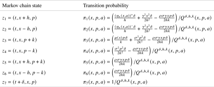
In Table 1, we define the Markov chain states and the associated transition probabilities that we obtain when we apply the finite difference approach.

TABLE 1.

The approximating Markov chain.

Thus, using the above notations and discretizing the space of controls as follows

$$\{0,\ldots,\bar{a}\} := \{a=(m-1)\bar{a}/(n_a-1), \; m=1,\ldots,n_a\},$$

where $n_a\in \mathbb {N}^{*}$, we approximate the HJB equations associated to the functions $v_0$ and $v_1$ for any $(x,p) \in [0,x_{{\rm max}}]\times [p_{{\rm min}},p_{{\rm max}}]$ by the following iterative scheme by starting with $v_0^{\delta,0}\equiv 0$ and $v_1^{\delta,0}\equiv 0$

$$v_0^{\delta,n+1}(t,x,p)=\frac{1}{1+\beta\Delta t^{\delta,h,k}(x,p,0)}\sum_{i=1}^{7}\pi_i(x,p,0)v_0^{\delta,n}(z_i) ,$$

for $t\in [0,T]- \{T_j\}_{1 \leq j \leq N}$,

$$v_0^{\delta,n+1}(T_j-\delta,x,p) = v^{\delta,n}_0(T_j,x,p){\mathbb 1}_{x \leq \Gamma} + v^{\delta,n}_1(T_j,x,p){\mathbb 1}_{x\gt \Gamma} ,$$

for $j\in \{1,\ldots,N-1\}$,

$$v_0^{\delta,n+1}(T_N-\delta,x,p) ={-}f((\Gamma -x)^{+},p)$$

and

$$v_1^{\delta,n+1}(t,x,p)=\max_{\{0, \ldots ,\bar{a}\}}\left\{\frac{\sum_{i=1}^{7}\pi_i(x,p,a)v_1^{\delta,n}(z_i)+(pa-C(a))\Delta t^{\delta,h,k}(x,p,a)}{1+\beta\Delta t^{\delta,h,k}(x,p,a)}\right\},$$

for $t\in [0,T]- \{T_j\}_{1 \leq j \leq N}$,

$$v_1^{\delta,n+1}(T_j-\delta,x,p) =v^{\delta,n}_0(T_j,x,p){\mathbb 1}_{x \leq \Gamma} + v^{\delta,n}_1(T_j,x,p){\mathbb 1}_{x\gt \Gamma},$$

for $j\in \{1,\ldots,N-1\}$,

$$v_1^{\delta,n+1}(T_N-\delta,x,p) ={-}f((\Gamma -x)^{+},p).$$

For any $(x,p) \in [0,x_{{\rm max}}]\times [p_{{\rm min}},p_{{\rm max}}]$, the above iterative scheme combined with the boundary conditions is explicit and fully implementable on the enlarged grid

\begin{align*} {\mathcal G}_{\delta,h,k}^{+} & :=\{t_i=(i-1)\delta, \; i=1,\ldots,n_t \}\times \{x_j=(j-1)h, \; j=0,\ldots,n_x+1\}\\ & \quad \times \{p_l=p_{{\rm min}}+(l-1)k, \; l=0,\ldots,n_p+1\} \end{align*}

with a given stopping criterion $\varepsilon$, that means the iterative scheme is stopped when the relative error is less than $\varepsilon$.

4.2. Numerical interpretations

The numerical computation are done using the following set of data.

• • Dynamics values

  • ◦ $\eta =0.7$, $\lambda =0.5$, $\gamma =0.2$, $\mu =0.1$, $\sigma =0.1$, $\rho =0.01$.

  • ◦ $T=1,\quad \beta =0.1$.

  • ◦ Drift function: $\mu (x)=\mu + 0.5 \times \exp (-0.2 x)$.

  • ◦ Penalty function : $f(x,p)=\kappa px$ with $\kappa =5$.

  • ◦ Cost function : $C(x)=x^{2}$.

  • ◦ Regulation parameters : $N=10\text { (number of checks)}, \quad \Gamma =0.2308$.

• • Grid values

  • ◦ Localization: $x_{{\rm max}}=1,\quad p_{{\rm min}}=0.1, \quad p_{{\rm max}}=1.1, \quad \bar {a}=0.5$.

  • ◦ Discretization: $n_x=40$, $n_p=40, \quad n_t=100, \quad n_a=10$.

  • ◦ Stopping criterion : $\varepsilon =0.01$.

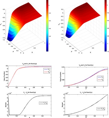
We plot the shape of the value functions $v_0$ and $v_1$ sliced in the plane $(x, p)$ for a fixed date $t$. We can see, as expected, $v_1\geq v_0$. In fact, we can see in line three of Figure 1 that the spread $v_1 - v_0$ is always positive. Obviously, if the manager can harvest the payoff will be greater. In the first graph of the second line of Figure 1, where we fix $(t,p)$, we can see that the two functions are nondecreasing w.r.t. $x$ which is natural due to the fact that greater the size of the natural resource, the more the manager can harvest and the less he/she is penalized at terminal time $T$. On the other hand, in the second graph of the second line of Figure 1, where we fix $(t,x)$ and take $x\gt\Gamma$, the two functions are nondecreasing in $p$, because the higher the price, the wealthier the manager becomes when he/she harvests and sells. Conversely, in the first line of Figure 1, when $x\lt\Gamma$, we can see that the value functions $v_0$ and $v_1$ are nonincreasing in $p$ which is due to the penalty function $f$ that is nondecreasing w.r.t. $p$ (i.e., the higher the price, the more the manager is penalized by the regulator).

FIGURE 1.

The shape of the value functions $v_0$ and $v_1$ for a fixed time $t$ (First Line). The shape of the value functions $v_0$ and $v_1$ for fixed $(t,p)$ and $(t,x)$ (Second Line). The spread between the value functions $v_0$ and $v_1$ for fixed $(t,p)$ and $(t,x)$ (Third Line).

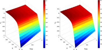
We plot the shape of the value functions $v_0$ and $v_1$ sliced in the plane $(t, x)$ for a fixed price $p$. In Figure 2, as expected, $v_0$ and $v_1$ are decreasing w.r.t. $t$ when $x$ is large. In fact, the manager will have more time to harvest the further he/she is from the terminal date $T$. If $x$ is small, the monotony depends on the parameters $\mu$ and $\eta$. On the one hand, when $x$ is small, we can see that $v_0$ and $v_1$ are increasing w.r.t. $t$ because the manager knows a priori that he/she is going to pay the tax since the quantity of natural resource will likely be smaller than $\Gamma$ at the terminal date $T$. On the other hand, if $t$ is small, the quantity of the natural resource increases with time, but so does the price, implying that the monotony of the value functions is not obvious. In fact, because $\mu$ is more important than $\eta$, the price in this case increases faster than the quantity of natural resource, so if the maturity is important, it is not beneficial for the manager because the tax will be more important.

FIGURE 2.

The shape of the value functions $v_0$ and $v_1$ for a fixed price $p$.

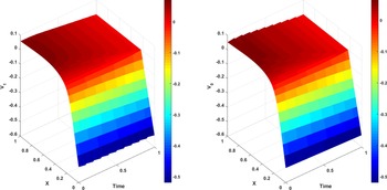
In Figure 3, we choose a smaller drift for the price. We remark that the monotony of the value functions $v_0$ and $v_1$ is the same as in the previous figure if $x$ is large. But now, the value functions $v_0$ and $v_1$ are decreasing when $x$ is small. This is because, unlike in Figure 2, the drift of the price is small, so the price increases more slowly than the available quantity of natural resource. Thus, if the maturity is important, it is advantageous for the manager. In fact, the tax will be less important since the quantity of natural resources available has had enough time to grow.

FIGURE 3.

The shape of the value functions $v_0$ and $v_1$ for a fixed price $p$ when $\mu (x)=0.01+0.05\times \exp (-0.002x)$.

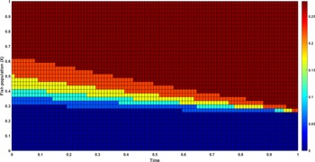
We plot the shape of the optimal harvest strategy $\alpha ^{*}(t,x,p)$ sliced in the plane $(x,t)$ for a fixed price $p$ (Figure 4). We can see two main regions: a harvest region (with different harvest rates) and a No-harvest region (dark blue). When we are far from maturity $T$, it is not optimal to harvest when $X$ is under $\lambda$ because under this quantity the resource quantity increases naturally so we want to let this happen to reach the maturity with $X$ greater than $\Gamma$ and thus avoid the penalization. As we get closer to $T$, it is best to harvest when $X\lt\lambda$ with different rates $a$, allowing us to reach $T$ without being penalized (i.e., $X_T\gt\Gamma$) and thus optimizing the profit generated by selling the harvest. The rates are greater as the natural resource population grows and this is due to the cost function $C$ (the cost of harvesting).

FIGURE 4.

The shape of the optimal control for a fixed price $p$.

In the following, we introduce a profit and loss measure, denoted P&L, defined as follows

$$\text{P & L}(\alpha) = \sum_{i=0}^{N-1}\sum_{t\in\mathcal{T}^{i}} e^{\beta (T-t)} (P^{\alpha}_{t}\alpha_{t}-\alpha_{t}^{2}) \delta\mathbb{1}_{X_{T_i}\gt\Gamma} - f((\Gamma - X^{\alpha}_T)^{+},P^{\alpha}_T),$$

where $\mathcal {T}^{i}:=\{T_i,T_i+\delta,\ldots,T_{i+1}\}$ with the convention $T_0=0$. In fact, this measure represents the payoff of the agent when adopting a given strategy $\alpha$. This measure will allow us to compare the effectiveness of the optimal control $\alpha ^{*}$ against a given naive strategy.

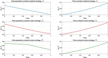
After computing the optimal strategy $\alpha ^{*}$ and the value function via the iterative procedure, we simulate the correlated Brownian motions $B$ and $W$ on the horizon $[0,T]$ and we adjust the dynamics of $X$ and $P$ according to the optimal control computed previously. Figure 5 represents a mean over 3,000 simulated paths of $X$ and $P$ controlled by the optimal strategy $\alpha ^{*}$ and two other naive strategies $\alpha ^{1}$ and $\alpha ^{2}$. The first naive strategy $\alpha ^{1}$ consists in harvesting the maximum $\bar {a}$ at all time when we are authorized till $T$ (in red) and the second one $\alpha ^{2}$ consists in waiting until a certain time $t_0$ which is chosen by the manager (in Figure 5 we take $t_0=0.5$) then harvesting the maximum $\bar {a}$ when we are authorized till time $T$ (in green). In Figure 5, the starting point is $X_0=0.7$ and $P_0=0.5$ and the P&Ls of the three strategies are respectively (with $95\%$ confidence level bounds): $\text {P & L}(\alpha ^{*})= 0.0873$ $(\pm 0.0002)$, $\text {P & L}(\alpha ^{1})= -0.0182$ $(\pm 0.0024)$, and $\text {P & L}(\alpha ^{2})=0.0315$ $(\pm 0.0005)$. We can see that our computed strategy is better than the two others. Indeed, with our strategy, the manager begins to harvest continuously at a rate $a$ smaller than the maximum $\bar a$, which allows him/her to attain terminal date $T$ with a natural resource population above $\Gamma$ avoiding the penalization that occurs if $X_T\lt\Gamma$. On the one hand, adopting the strategy $\alpha ^{1}$, the manager at time $T$ harvests more but he/she is penalized because the quantity of resource is under $\Gamma$ at the terminal time $T$. On the other hand, using the strategy $\alpha ^{2}$, he/she is not penalized because the quantity of resource at time $T$ is above $\Gamma$ but he/she harvests for a shorter period of time (starting the harvesting at $t_0=0.5$), hence, resulting in lower revenue.

FIGURE 5.

The optimal control $\alpha ^{*}$ vs naive controls $\alpha ^{1}$ and $\alpha ^{2}$.

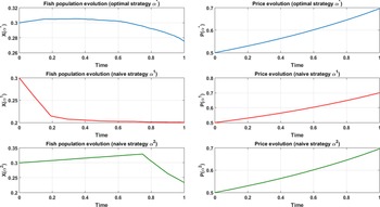
As in Figure 5, Figure 6 represents a mean over 3,000 simulated paths of $X$ and $P$ for the optimal control and the same two other naive strategies. But this time we choose to start with $X_0=0.3$ and $P_0=0.5$. The P&Ls of the three strategies are respectively (with $95\%$ confidence level bounds): $\text {P & L}(\alpha ^{*})=0.0302$ $(\pm 0.0008)$, $\text {P & L}(\alpha ^{1})= -0.1032$ $(\pm 0.0027)$, and $\text {P & L}(\alpha ^{2})=-0.0331$ $(\pm 0.0022)$. We can see that our strategy is still better than the two others. On the one hand, starting at time $t=0$ from a position under the threshold $\lambda$, the natural resource population tends to increase (mean-reverting effect), hence, as we can see in Figure 6, our optimal strategy is to wait until $X$ reaches a certain level over $\Gamma$ before starting to harvest (around time $t=0.2$). Doing this allows the manager to avoid the risk of being under the penalization barrier $\Gamma$ at time $T$. On the other hand, using the first naive strategy $\alpha ^{1}$, the natural resource population is quickly under $\Gamma$ and at time $t=0.2$, the regulator does not allow the manager to harvest anymore. Moreover, the manager is penalized as the natural resource population does not surpass $\Gamma$ at time $T$. On the contrary, if we wait up to time $t_0=0.75$ before starting to harvest with the maximum rate $\bar {a}$ (the naive strategy $\alpha ^{2}$), the natural resource population grows (since $X_t\lt\lambda$) till time $t_0=0.75$ and then decreases (because the harvesting starts at this date) but will be above $\Gamma$ at time $T$. Hence, we are not penalized but still our optimal strategy $\alpha ^{*}$ outperforms $\alpha ^{2}$ in terms of P&Ls.

FIGURE 6.

The optimal control $\alpha ^{*}$ vs naive controls $\alpha ^{1}$ and $\alpha ^{2}$ ($X_0=0.3$ and $P_0=0.5$).

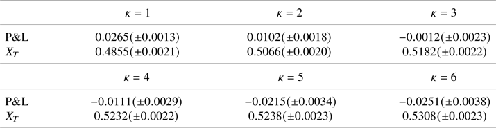
In Table 2, we choose to compute our optimal strategy and the corresponding simulations for $\Gamma =0.4872\gt\lambda =0.3$. With this configuration, we know that if the natural resource population drops under $\Gamma$, it is likely to stay under $\Gamma$. Therefore, the manager is obligated to keep the natural resource population $X$ over $\Gamma$ at all times in order to avoid the penalization at the maturity $T$. Except for $\Gamma$ and $\lambda$, we use the same values of the parameters defined in the beginning of this numerical part and we represent in Table 2 the value of the P&L and the natural resource population $X$ at time $T$ starting with $X_0=0.7$ and $P_0=0.5$. These quantities were computed using a mean over 3,000 trajectories under the optimal control $\alpha ^{*}$ for different values of the penalty constant $\kappa$ (with $95\%$ confidence level bounds). We can see that the P&L is a decreasing function w.r.t. $\kappa$ which is natural because the less the manager is penalized, the more he/she takes risks and the richer he/she is. Although we can remark that for $\kappa =1$ the natural resource population at time $T$ is under $\Gamma$ because the penalization is not severe enough, hence the manager prefers to be penalized and harvests a little more which makes him/her richer. Therefore, we assume that for our set of data, to create a fair balance between the biological requirements and the maximization of the profit induced by harvesting, a suitable choice for the penalty constant is $\kappa =2$. This amount of fines insures the double objective of the sustainable harvesting: the natural resource population does not fall below a certain threshold that guarantees its natural renewal, and the manager makes profits to prevent him/her from going bankrupt.

TABLE 2.

P&L for different penalty constant $\kappa$.