

1. Introduction
We are interested in modeling dense weighted networks with real, continuous-valued weights
 $W_{uv}$
for pairs of nodes
 $u$
,
 $v \in V$
, where
 $V$
denotes the set of all nodes (vertices) in the network. Denseness means that the edge
 $W_{uv}$
is present for all pairs
 $u$
,
 $v$
where
 $u \ne v$
, though we will also discuss the case where a proportion of the weights are “missing.” Examples include structural brain networks (as in Figure 1) and correlation networks. Focusing on dense weighted networks, what are natural modeling approaches? At the simplest level, if a network has no meaningful structure, one could postulate that
 \begin{equation} f(W_{uv}) = \varepsilon _{uv}, \end{equation}
where
 $\varepsilon _{uv}$
are i.i.d.
 $\mathcal{N}$
 $(0, 1)$
random variables and
 $f$
is a function mapping
 $W_{uv}$
to the (standard) “normal” space. One can take
 \begin{equation} f(w) = \Phi ^{-1}(G(w)), \end{equation}
where
 $G$
is the CDF of
 $W_{uv}$
and
 $\Phi ^{-1}$
is the inverse CDF of
 $\mathcal{N}$
 $(0, 1)$
. In practice, we can substitute the empirical CDF for the unknown true
 $G$
.
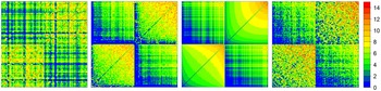
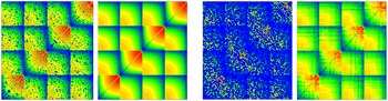
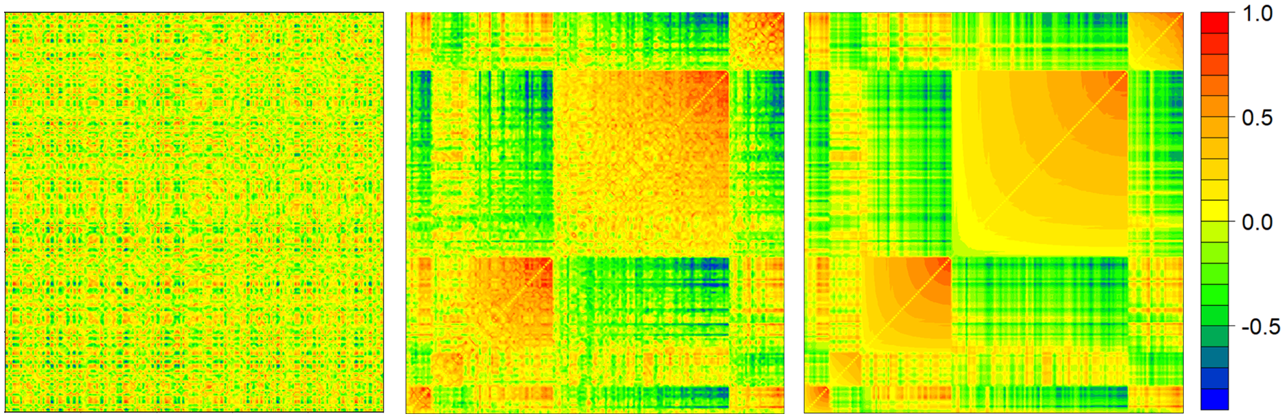
From left to right: a structural brain network of the log values of white matter fiber counts between 148 regions. The same network reordered by within community degree. The similarly reordered “estimate” of the structural network. A reordered bootstrap replicate network of the observed network.
Most networks of interest, including most real networks, however, have some kind of structure. Two common structures involve communities, broadly understood as sets of particular nodes whose edges exhibit similar connectivity patterns, and degree heterogeneity, broadly understood as certain nodes having consistently more edges (or, in dense weighted networks, greater edge weights) than other nodes. Degree correction is a means of accounting for degree heterogeneity. A simple way to capture degree correction, which we refer to as “sociability” (or SC, for short) in the “normal” space, is to set
 \begin{align} f(W_{uv}) & = \alpha Z_u + \beta Z_v + \sigma \varepsilon _{uv} \nonumber \\ & = \alpha \Phi _1^{-1}(\Psi _u) + \beta \Phi _1^{-1}(\Psi _v) + \sigma \varepsilon _{uv} \,=\!:\, h(\Psi _u, \Psi _v) + \sigma \varepsilon _{uv}, \end{align}
where
 $Z_u$
and
 $Z_v$
are i.i.d.
 $\mathcal{N}$
 $(0, 1)$
variables, associated with nodes
 $u$
and
 $v$
, respectively, and
 $\alpha, \beta$
and
 $\sigma$
are other model parameters. In the equivalent expression,
 $\Psi _u$
are i.i.d. U
 $(0, 1)$
random variables (uniform on the interval
 $(0, 1)$
), and the function
 $h(x, y) = \alpha \Phi ^{-1}(x)+ \beta \Phi ^{-1}(y)$
will be allowed to take more general forms below. In the “normal” space, the function
 $h(\Phi (z_u), \Phi (z_v)) = \alpha z_u + \beta z_v$
is linear. In the case where
 $\alpha, \beta \gt 0$
, a larger value of
 $Z_u$
will tend to make
 $W_{uv}$
values larger across all
 $v$
’s, inducing a sociability structure that reflects degree correction. The term
 $h(\Psi _u, \Psi _v)$
in (3) is thus the SC term in the model. The term
 $ \sigma \varepsilon _{uv}$
is thought to consist of independent
 $\mathcal{N}$
 $(0,\sigma ^2)$
variables.
Models of the type (3) appear in Fosdick & Hoff (Reference Fosdick and Hoff2015), who also include a multiplicative interaction term. In a departure from that work, we allow for community structures and more general functions
 $h$
than (3). After exponentiation, and at the conditional mean level, note also that (3) yields
 \begin{equation} \mathbb{E}\!\left(e^{\,f(W_{uv})}|Z\right) = e^{\alpha Z_u}e^{\beta Z_v}e^{\frac{\sigma ^2}{2}} \,=\!:\, \theta _u\theta _v \mu . \end{equation}
Specifications of the form (4) are common for connection probabilities in unweighted degree corrected or SC models. See degree corrected stochastic block models (DCBMs) in Karrer & Newman (Reference Karrer and Newman2011), Gao et al. (Reference Gao, Ma, Zhang and Zhou2018), or their extensions, popularity adjusted stochastic block models (PABMs) in (Sengupta & Chen Reference Sengupta and Chen2017), (Noroozi et al. Reference Noroozi, Rimal and Pensky2021). While in the DCBM, “sociability” parameters are global, in the PABM, each node has a possibly different sociability parameter for each community in the network. The models considered here are close in spirit to PABMs, and we draw from the techniques in Noroozi et al. (Reference Noroozi, Rimal and Pensky2021) to analyze them. However, our focus is on weighted networks where information may be encoded in the patterns of the edge weights rather than the existence of particular edges in a given network. We shall thus also consider community versions of the model (3), where the function
 $h$
and the parameter
 $\sigma$
can depend on the pair of communities to which
 $u$
and
 $v$
belong. Importantly, according to this definition, communities are not necessarily defined by higher or lower propensities to connect with entire other communities, but rather by particular patterns of edge weights which represent “preferences” for specific nodes over others within the same community.
As noted above, we will go beyond the “linear” sociability patterns encoded by the particular function
 $h$
shown in (3) while, perhaps surprisingly, remaining in the “normal” space. To motivate this extension, instead write the SC term in (3) as
 \begin{equation} h(\Psi _u, \Psi _v) = d \Phi ^{-1}(H(\Psi _u, \Psi _v)), \end{equation}
where
 $d \in [0,1]$
and
 $H(x,y) = \Phi (c^{-1}\alpha \Phi ^{-1}(x) + c^{-1}\beta \Phi ^{-1}(y))$
with
 $c = \sqrt{\alpha ^2 + \beta ^2}$
.
 $\alpha$
and
 $\beta$
modulate the influence of
 $y$
relative to
 $x$
. The constant
 $c$
serves a normalizing role so that
 $H(\Psi _u, \Psi _v)$
is ensured to be U
 $(0, 1)$
, and hence, the value of
 $h(\Psi _u, \Psi _v)$
resides in the “normal” space with variance
 $d^2$
. Plugging (5) into the last term of (3) and constraining
 $d^2 + \sigma ^2 =1$
ensures the resulting values of
 $f(W_{uv})$
are in the (standard) “normal” space.
The critical observation, though, is that plugging (5) into (3) while constraining
 $d^2 + \sigma ^2 =1$
will output values in the (standard) “normal” space for any function
 $H$
where
 $H(\Psi _u, \Psi _v) \sim$
U
 $(0, 1)$
, including functions that bear no similarity to the normal distribution as shown beneath (5). We shall consider several broad classes of such
 $H$
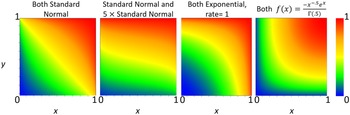
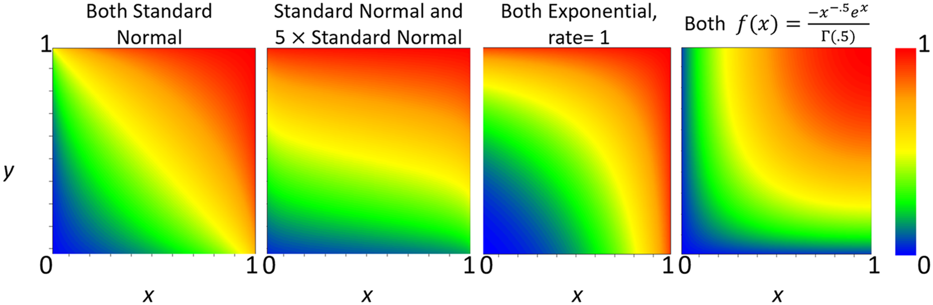
-functions. Examples of the sociability patterns resulting from various considered
 $H$
-functions are depicted in Figure 2 below. The key point is that while
 $H$
could be associated with quite different SC patterns, the SC term (5) would nonetheless reside in the “normal” space. Used in conjunction with (2), which transforms an arbitrary (and possibly nonparametric) distribution of edge weights, this constructs a map between
 $\Psi$
values and edge weights via the (standard) “normal” space. In summary, our key contributions at the model level concern:
-
Focus on dense weighted networks;
-
Possibility of community structure;
-
Multiple nearly arbitrary distributions of edge weights;
-
Flexible sociability patterns through
 $H$
-functions.

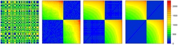
Plots of examples of
 $H$
-functions.
Modeling questions will also be addressed in the paper below. Figure 1 illustrates our modeling approach. It shows a network where the edge weights are the logs of the white matter fiber counts connecting two regions in a patient’s brain. In this case, the two assumed communities are the left and right hemispheres of the brain. We often reorder the nodes first by community and then, within each community, sort the nodes by within community degree. This is what is seen in the second plot from the left of Figure 1. There are instances where one might want to sort the nodes differently, for example, if there is a core-periphery structure, it might be preferable to sort nodes first by community then by weight of edges connected to nodes in the core. In the third plot from the left, we show an “estimate” of the SC term from our method, with the same ordering as in the second plot. Finally, a bootstrap replicate network of the original network is displayed in the right plot, again reordered for easier viewing. Notably, based on the different contour shapes in the bottom left and the top right sections of the third plot, it can be seen (using the plots in Figure 2 as a point of reference) that the intra-left hemisphere edges have a different best fitting
 $H$
-function than the intra-right hemisphere edges.
There are other models designed to generate weighted networks. The Weighted Stochastic Block Model introduced by Aicher et al. (Reference Aicher, Jacobs and Clauset2013) includes degree correction only with regard to an edge’s existence, not for modeling the weights of particular edges. The generalized exponential random graph model from Desmarais & Cranmer (Reference Desmarais and Cranmer2012a) is indeed a very general model, but requires a lot of advanced knowledge to specify the appropriate model for estimation if given a specific network. As noted above, Fosdick & Hoff (Reference Fosdick and Hoff2015) includes a form that looks superficially like the linear models discussed in this paper, but the higher order dynamics described when incorporating multiplicative interaction effects bears little resemblance to the “non-linear” models presented here and does not accommodate communities. Peixoto (Reference Peixoto2018) looks for general forms of community structure, but not of the kind proposed here, as their edge weights depend only on community membership without regard for other nodal features. For other work on weighted networks, see the melding of mutual information and common neighbors in Zhu & Xia (Reference Zhu and Xia2016), estimates of nodes’ perceptions of one another to predict signed edge weights in Kumar et al. (Reference Kumar, Spezzano, Subrahmanian and Faloutsos2016), and leveraging graph metrics to “denoise” weighted networks in Spyrou & Escudero (Reference Spyrou and Escudero2018). Related work in the unweighted setting can be found in Bartlett (Reference Bartlett2017), which deploys pairwise measures of node association to model binary edges, and the use of copulas in Fan et al. (Reference Fan, Xu and Cao2016).
As seen in Figure 1, for a given network, we can use our model to estimate a data generating process and subsequently generate synthetic data via a bootstrap-type method. This procedure can create “new” networks which replicate the structure of the observed network even without a priori knowing the functional form of the edge weight generating process between particular communities. As in the case of using brain networks as a diagnostic aid, when networks are used as inputs to other analyses, if data collection is difficult, these synthetic network replicates may be used as supplemental data. Additionally, taking a cue from the rightmost plot of Figure 1, the random variation between bootstrap replicate networks can serve as a sensitivity test for results using the original network, allowing for greater robustness even with limited data, as in the classical bootstrap.
The rest of this paper is structured as follows. In Section 2, we develop theory for generating the proposed class of networks, along with details on
 $H$
-functions in Section 3. In Section 4, we discuss methods for estimating the generating processes of observed networks when the community memberships of each node are known or have been estimated. In Section 5, we build on the estimation procedures from Section 4 to generate new synthetic networks that are plausible stand-ins for real networks, in the vein of the bootstrap. In Section 6, we discuss how to adapt community detection techniques to networks of this kind. In Section 7, we discuss applying our methods under slight departures from the main models of interest. In Section 8, we apply our method to real data and compare the performance to other existing models. The supplementary appendix to the paper (Leinwand & Pipiras Reference Leinwand and Pipiras2022) discusses technical details and extensions.
2. Model formulation
Let
 $v_1,\ldots, v_n$
be the vertices (nodes) in a dense network with undirected and weighted edges, and no self-loops. Each node belongs to exactly one community,
 $1, \ldots, K$
. Henceforth,
 $u$
and
 $v$
will refer to nodes, and
 $i$
and
 $j$
will refer to communities, for example
 $u \in i, v \in j$
.
In our random graph model, a node
 $u$
has a “sociability” (i.e. “popularity,” degree correction) parameter
 $\Psi _u$
. These parameters are assumed to be i.i.d. U
 $(0, 1)$
. Let
 $W_{u v}$
denote the weight of the edge connecting nodes
 $u$
and
 $v$
. We primarily focus on the case with continuous-valued
 $W_{u v}$
. At the most general level, we examine random graphs of the following form: for
 $u, v$
such that
 $u \in i$
,
 $v \in j$
, suppose
 \begin{equation} f_{ij}(W_{u v}) = h_{i j}(\Psi _{u}, \Psi _{v}) + \sigma _{ij}\varepsilon _{uv}, \end{equation}
where
 $f_{ij}$
is a monotonically increasing function over the range of
 $W_{uv}$
,
 $h_{ij}$
is a monotonic function in its 2 arguments,
 $\varepsilon _{uv}$
are error terms with
 $\mathbb{E}(\varepsilon _{uv}) = 0$
,
 $\mathbb{E}(\varepsilon _{uv}^2) = 1$
and
 $ \sigma _{ij} \ge 0$
. Those terms with
 $ij$
subscripts are particular to edges where one of the nodes is in community
 $i$
and the other is in community
 $j$
, while terms with subscripts
 $uv$
are idiosyncratic for that particular edge. In the most flexible version of the model, as in the PABM, each node may have
 $K$
different
 $\Psi$
values, each one for parametrizing edge weights connecting to nodes in a particular community. A special case of interest is the linear model
 \begin{equation} f_{ij}(W_{u v}) = \gamma _{i j} + \alpha _{ij}h_{1ij}(\Psi _u) + \beta _{ij}h_{2ij}(\Psi _v) + \sigma _{ij}\varepsilon _{uv}, \end{equation}
where
 $ \gamma _{i j}, \alpha _{ij}, \beta _{ij} \in \mathbb{R}$
,
 $\mathbb{E}(h_{kij}(\Psi )) = 0$
, and
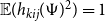 $\mathbb{E}(h_{kij}(\Psi )^2) = 1$
for
 $k = 1,2$
and
 $\Psi \sim$
U
 $(0, 1)$
. We refer to (7) as a linear sociability model (LSM) and to (6) where
 $h_{ij}$
is not linear as a non-linear sociability model (NSM). Examples and discussion below will provide motivation and intuition about these models.
Under monotonicity assumptions, note that the observed edge weight
 $W_{uv}$
is monotone in the sociability parameters of nodes
 $u$
and
 $v$
. As a special case, letting
 $\alpha _{ij} = \beta _{ij} = 0$
in the LSM, node sociability plays no role in the weight of the edge between nodes
 $u$
and
 $v$
, rather the weights are generated independently from some distribution, as in a Weighted Stochastic Block Model. Similarly, letting
 $\sigma _{ij} = 0$
would generate a network completely determined by random node sociabilities.
One natural choice of
 $f$
in (6) or (7), after a common practice of transforming data to standard normal, is to consider
 \begin{equation} f(w)= \Phi _1^{-1}(G(w)), \end{equation}
where
 $G$
represents the CDF of
 $\{W_{uv}\,:\, u \in i, v \in j\}$
. We pursue this case in the following canonical example that we use for NSMs. The example relies upon H-functions, a concept that will be discussed in greater detail in Section 3.
In what follows,
 $\Phi _{\mu,\sigma ^2}$
will denote the CDF of a
 $\mathcal{N}(\mu, \sigma ^2)$
distribution and
 $\Phi _{\sigma ^2} \,:\!=\, \Phi _{0,\sigma ^2}$
. Furthermore, though each pair of communities
 $i$
and
 $j$
are assumed to possibly be connected via a function
 $h_{ij}$
(along with
 $\gamma _{i j}, \alpha _{ij}, \beta _{ij}$
, etc.), to simplify notation, we will drop the subscript in our notation, assuming that the discussion always concerns the relevant pair of communities
 $i, j$
based on context, where
 $i$
may or may not be the same as
 $j$
.
Example 1. (
 $H$
-Normal NSM.) This is (6) with
 \begin{equation} \Phi _1^{-1}(G(W_{uv})) = \frac{1}{\sqrt{1+\sigma ^2}} \Phi _1^{-1}(H(\Psi _u, \Psi _v))+ \frac{\sigma }{\sqrt{1+\sigma ^2}} \varepsilon _{uv}, \end{equation}
where
 $G$
is again the CDF of
 $W_{uv}$
,
 $\varepsilon _{uv}$
are i.i.d.
 $\mathcal{N}(0, 1)$
, and
 $\sigma \ge 0$
. Furthermore,
 $H(x, y)$
is an
 $H$
-function having the following key properties (see Section 3 for more details):
 $H(\Psi _u, \Psi _v) \sim$
U
 $(0, 1)$
for independent U
 $(0, 1)$
random variables
 $\Psi _u, \Psi _v$
, and
 $H(x, y)$
is monotone in both arguments. The first property ensures that
 \begin{equation} \frac{1}{\sqrt{1+\sigma ^2}} \Phi _1^{-1}(H(\Psi _u, \Psi _v)) + \frac{\sigma }{\sqrt{1+\sigma ^2}} \varepsilon _{uv}\ \,=\!:\, Z_{uv} \end{equation}
are
 $\mathcal{N}(0, 1)$
variables, and hence by inverting (9), the variables
 \begin{equation} W_{uv} = G^{-1}(\Phi _1(Z_{uv})) \end{equation}
indeed have
 $G$
as their CDF.
Example 2. (Normal LSM.) This is (7) with
 \begin{align} f(W_{uv}) & = \gamma + \alpha \Phi _1^{-1}(\Psi _u) + \beta \Phi _1^{-1}(\Psi _v) + \sigma \varepsilon _{uv} \nonumber \\ & = \gamma + \alpha Z_u + \beta Z_v + \sigma \varepsilon _{uv}, \end{align}
where
 $Z_u \sim \mathcal{N}(0, 1)$
. The function
 $f$
can be the identity (in which case
 $W_{uv}$
is Gaussian itself, assuming normality of
 $\varepsilon _{uv}$
) or some other transformation, such as
 $f(W) = \log \!(W)$
.
The Normal LSM with
 $f$
as in (8) is a special case of the
 $H$
-Normal NSM. Using the
 $H$
-function
 \begin{equation} H(x, y) = \Phi _{1+\rho ^2}\!\left(\Phi _1^{-1}(x) + \Phi _{\rho ^2}^{-1}(y)\right), \end{equation}
one observes that
 $H(\Psi _u, \Psi _v) \sim$
U
 $(0, 1)$
since
 $\Phi _1^{-1}(\Psi _u) \sim \mathcal{N}(0, 1), \Phi _{\rho ^2}^{-1}(\Psi _v) \sim \mathcal{N}\!\left(0, \rho ^2\right)$
, and hence
 $\Phi _1^{-1}(\Psi _u) + \Phi _{\rho ^2}^{-1}(\Psi _v) \sim \mathcal{N}(0, 1+\rho ^2)$
. With the choice (13) plugged into (9), the latter model becomes
 \begin{align} \Phi _1^{-1}(G(W_{uv})) & = \frac {1}{\sqrt {1+\sigma ^2}} \Phi _1^{-1}(H(\Psi _u, \Psi _v))+ \frac {\sigma }{\sqrt {1+\sigma ^2}} \varepsilon _{uv}\nonumber\\[4pt]& = \frac {1}{\sqrt {1+\sigma ^2}} \!\left ( \Phi _1^{-1}\!\left(\Phi _{1+\rho ^2}\!\left(\Phi _1^{-1}(\Psi _u) + \Phi _{\rho ^2}^{-1}(\Psi _v)\right)\right) \right )+ \frac {\sigma }{\sqrt {1+\sigma ^2}} \varepsilon _{uv}\nonumber\\[4pt]& =\frac{1}{\sqrt{1+\sigma ^2} \sqrt{1+\rho ^2}} \Phi _1^{-1}(\Psi _u) + \frac{\rho }{\sqrt{1+\sigma ^2 }\sqrt{1+\rho ^2}} \Phi _1^{-1}(\Psi _v) + \frac{\sigma }{\sqrt{1+\sigma ^2}} \varepsilon _{uv}, \end{align}
by using the identities
 $\Phi _a^{-1}(c) = \sqrt{a}\Phi _1^{-1}(c)$
and
 $\Phi _b(c) = \frac{\Phi _1(c)}{\sqrt{b}}$
. Note that (14) is a normalized version of the Normal LSM (3) where
 $\gamma$
is set to 0. Examples of
 $H$
-functions which do not correspond to Normal LSM will be given in Section 3. NSMs are a large class, but some other potentially interesting examples can be constructed in a similar manner to the
 $H$
-Normal NSM above, as is detailed in the technical appendix (Leinwand & Pipiras Reference Leinwand and Pipiras2022).
While
 $H$
-Normal NSMs indeed take advantage of many features of the normal distribution, they are actually not very restrictive. Instead of representing the CDF of a linear combination of normal random variables as in (13), the
 $H$
-function in (9) can represent the CDF of some other weighted combination of random variables, in which case the underlying “shape” of the connections between communities
 $i$
and
 $j$
will look very different, as can be seen in Figure 2. This paper will focus on
 $H$
-Normal NSMs because all
 $H$
-Normal NSMs incorporate normally distributed errors. The special case of Normal LSMs is discussed further in the appendix.
Finally, we introduce a bit more terminology. In the LSM (7), we distinguish the following cases with specific terms:
-
$\alpha \gt 0$
,
$\beta \gt 0$
: positive association,
-
$\alpha \lt 0$
,
$\beta \lt 0$
: negative association,
-
$\alpha \cdot \beta \lt 0$
: Simpson association,
-
$\alpha \ne 0$
,
$\beta = 0$
: projection onto 1st coordinate,
-
$\alpha = 0$
,
$\beta \ne 0$
: projection onto 2nd coordinate.


3.
$H$
-functions

We begin by introducing some terminology.
Definition 1. (Positive association.) A function
 $H\,:\,(0, 1) \times (0, 1) \rightarrow (0, 1)$
is an
 $H$
-function with positive association if:
-
1.
$H$
is non-decreasing in both arguments;
-
2.
$\iint _{H(x, y)\le z} dx dy =z$
, for all
$z \in (0, 1)$
.



The term “positive association” refers to the fact that, when considered across communities, such models would tend to produce larger weights for nodes in the two communities with simultaneously larger sociabilities. The monotonicity condition 1 captures the idea of node sociability as discussed above. Condition 2 is equivalent to requiring that
 $H(\Psi _u, \Psi _ v) = \Psi _{u v}$
is a U
 $(0, 1)$
random variable. In contrast with copulas, the output of a positively associated
 $H$
-function is not bounded above by the minimum of the inputs.
Definition 2. (Negative association; Simpson association.) A function
 $H\,:\,(0, 1) \times (0, 1) \rightarrow (0, 1)$
is an
 $H$
-function with negative association if
 $H(1-x, 1-y)$
is an
 $H$
-function with positive association. A function
 $H\,:\,(0, 1) \times (0, 1) \rightarrow (0, 1)$
is an
 $H$
-function with Simpson association if
 $H(x, 1-y)$
or
 $H(1-x, y)$
is an
 $H$
-function with positive association.
If
 $\Psi _u$
is a uniform random variable, then
 $1-\Psi _u$
is also a uniform random variable, so negative association also ensures that
 $H(\Psi _u, \Psi _ v) = \Psi _{u v}$
is a uniform random variable. A similar observation can be made for Simpson association. The term “negative association” arises because the monotonicity of
 $H$
results in the fact that, when looking across the communities, nodes with greater node sociabilities actually tend to have smaller edge weights. Simpson associations are so named because they indicate a localized area where certain broader trends of the network may be inverted. This error at the local level when extrapolating from global phenomena is reminiscent of Simpson’s paradox.
A property shared by all
 $H$
-functions is that
 $H(\Psi _{u}, \Psi _{v})$
is a U
 $(0, 1)$
random variable for such independent random variables
 $\Psi _u, \Psi _v$
. There are many ways to achieve this, but one quite general construction which we found to be flexible and interesting is as follows. Note that a random variable
 $F^{-1}(\Psi )$
has the CDF
 $F$
for a U
 $(0, 1)$
random variable
 $\Psi$
. Take now two CDFs
 $F_1, F_2$
and let
 $F_{1,2} = F_1 * F_2$
be their convolution CDF. Then,
 $F_1^{-1}(\Psi _u) + F_2^{-1}(\Psi _v)$
has the same distribution as
 $F_{1,2}^{-1}(\Psi _{u v})$
. This suggests setting
 \begin{equation} H(x, y) = F_{1,2}\!\left(F_1^{-1}(x) +F_2^{-1}(y)\right). \end{equation}
By construction, this function satisfies the condition 2 of Definition 1, but one can easily check that condition 1 holds as well. The function (13) is an example of
 $H$
-function in the form of (15) with an explicit convolution
 $F_{1,2}$
. Besides the normal distributions, choosing
 $F_1$
and
 $F_2$
to be exponential, Cauchy, or uniform would also give an explicit form for
 $F_{1,2}$
, although (15) is far more general than these simple cases imply.
Figure 2 illustrates some of the different kinds of contours that can be created using
 $H$
-functions of the form in (15). The resulting weighted bipartite subnetworks between 2 different communities generated using these
 $H$
-functions in
 $H$
-Normal NSM (9) would inherit similar connectivity patterns, albeit with normally distributed “errors” included. In this case, the x and y axes represent the values of
 $x$
and
 $y$
, respectively, each running from 0.01 to 0.99 by increments of 0.01, and the colors represent the output of the
 $H$
-function. From left to right, the first plot shows the values of
 $H(x, y) = \Phi _{1+\rho ^2}\!\left(\Phi _1^{-1}(x) + \Phi _{\rho ^2}^{-1}(y)\right)$
where
 $\rho =1$
. The second plot corresponds to this function with
 $\rho = 5$
. The third plot depicts (15) where
 $F_1$
and
 $F_2$
are both exponential distributions with a rate parameter 1, and
 $F_{1,2}$
is a gamma distribution with shape parameter of 2 and rate parameter of 1. Finally, the rightmost plot is from the
 $H$
-function (15) where
 $F_1$
and
 $F_2$
have density
 \begin{equation*}f(x) = \begin {cases} \frac {-x^{-.5}e^x}{\Gamma (.5)}, & x\lt 0, \\[5pt] 0, & \text {otherwise}. \end {cases} \end{equation*}
In this case,
 $F_{1,2}$
can be checked to be given by
 \begin{equation*}F_{1,2}(z) = \begin {cases} e^{z}, & z\lt 0, \\[4pt] 1, & z\ge 0 . \end {cases} \end{equation*}
These different images show that
 $H$
-functions (15) make a rather flexible class. Other
 $H$
-functions include maps to the first or second coordinates, which would give perfectly vertical or horizontal contours.
4. Estimation with known communities
In this section, we discuss estimation of
 $H$
-Normal NSMs, while assuming that the true community labels
 $\{ i \}$
of the nodes in the network are known. Our proposed approach to community detection is deferred to Section 6. The presentation below does not include any theoretical results. We see a straightforward path to obtain such results but are currently missing the Glivenko-Cantelli (law of large numbers) and more refined foundational limit results for the
 $\{W_{uv}\}$
having spatial dependence over
 $u, v$
stemming from their definition (9). Nevertheless, simulation results in Section 8 and Appendix E demonstrate the estimation procedure can recover underlying structures from a wide variety of models and, as expected, performs better with more nodes and smaller
 $\sigma$
values.
According to (9), all of
 $G$
,
 $\{ \Psi \}$
,
 $H$
, and
 $\sigma$
must be estimated for the
 $H$
-Normal NSM. In our estimation process, we do not impose that each node’s estimated
 $\widehat{\Psi }_u$
value is constant globally, but rather only constant over each community. It may be desirable in future work to align these
 $\widehat{\Psi }_u$
estimates over the whole network, but the presented estimation processes are more flexible. Even using this assumption, the model parameters to be estimated depend on the specific model in question. Given a particular set of community labels, we can treat each subnetwork of the larger network—where we analyze the connectivity patterns between 2 different communities
 $i$
and
 $j$
—as a bipartite graph, and any subnetwork where we look at the connectivity within a single community as a smaller network.
Remark: The discussion of our models is supplemented in Appendices A and B by the following two developments. Estimation for (Normal) LSMs using non-negative matrix factorization is discussed in Appendix A. In Appendix B, we provide concentration inequalities for Normal LSMs that are estimated through an
 $L_2$
loss, including the estimation of communities, with a penalty term based on the number of nodes and the number of communities in the network. The linearity, low-rank structure, and sub-Gaussianity are key assumptions in the proofs of the inequalities, making their extension to
 $H$
-Normal NSMs outside immediate but possibly within future reach.
4.1 Estimation for
$\textbf{H}$
-Normal NSM

We assume henceforth that
 $i$
and
 $j$
are fixed and work on one smaller subnetwork. For an estimator of
 $G_{ij}$
, by the construction of the graph in the
 $H$
-Normal NSM (9), one could naturally set the empirical CDF of the weights
 $\{W_{uv}\,:\, u \in i, v \in j\}$
. We make a small modification to this and instead set
 \begin{equation} \widehat{G}(w) = \frac{1}{n+1}\sum _{W_{uv}\,:\, u \in i, \, v \in j} \mathbb{1}_{\left\{W_{uv}\le w\right\}}\,, \end{equation}
where
 $n$
is the number of edges
 $W_{uv}\,:\, u \in i, v \in j$
. That is, we divide by
 $n+1$
in (16) instead of
 $n$
. There are two reasons for this. First, note that the model in (9) implies a distorted but generally linear relationship between
 $\Phi _1^{-1}(G(W_{uv}))$
and
 $\Phi _1^{-1}(H(\Psi _u, \Psi _v))$
. We shall use this relation to estimate the function
 $H$
, and at the empirical level, shall consider
 $\widehat{G}(W_{uv})$
in place of
 $G(W_{uv})$
. Dividing by
 $n+1$
ensures that
 $\widehat{G}(W_{uv}) \lt 1$
, so
 $\Phi _1^{-1}(\widehat{G}(W_{uv}))$
is finite. Second, modulo any dependence issues, if one thinks of (an appropriate scaling of)
 $H(\Psi _u, \Psi _v)$
as representing the order statistics of
 $n$
uniform random variables on (0, 1), recall that the
 $k$
th order statistic follows a Beta
 $(k, n+1-k)$
distribution, which has a mean of
 $\frac{k}{n+1}$
. At the mean level, it is then natural to place
 $\widehat{G}(W_{uv})$
at multiples of
 $\frac{1}{n+1}$
, not
 $\frac{1}{n}$
. In fact, we use one other modification to the definition (16) when the values
 $W_{uv}$
repeat, which can be found in Appendix C of Leinwand & Pipiras (Reference Leinwand and Pipiras2022).
For node sociabilities
 $\Psi _u$
, we define them locally based on two communities
 $i$
and
 $j$
(and possibly
 $i=j$
so there is only one community). For node
 $u \in i$
, consider
 \begin{equation} D_{j}(u) = \sum _{v\,:\, v \in j}\Phi _1^{-1}\!\left(\widehat{G}\!\left(W_{uv}\right)\right). \end{equation}
We think of
 $D_{j}(u)$
as a “local sociability statistic” of
 $u$
, since it looks at how
 $u$
connects to one community
 $j$
, rather than the whole network. By the construction of the NSM model (9) and the properties of positively associated
 $H$
-functions, if
 $H$
is positively associated, one expects the ordering of the local sociability statistics
 $D_{j}(u)$
’s of those nodes in community
 $i$
to match the ordering of the sociabilities
 $\Psi _u$
. This suggests setting
 \begin{equation} \widehat{\Psi }_u^{(j)} = \frac{1}{n_i+1}\sum _{u^{\prime}\,:\, u^{\prime} \in i} \mathbb{1}_{\left\{D_j\!\left(u^{\prime}\right)\le D_j(u)\right\}}, \end{equation}
where
 $n_i$
is the number of
 $u^{\prime} \,:\, u^{\prime} \in i$
. That is, defining
 $\widehat{\Psi }_u^{(j)}$
as the rescaled ordering of the “local sociability statistic” of
 $u$
in its community
 $i$
with respect to community
 $j$
. As in (16), note the division by
 $n_i +1$
in (18), placing the
 $\widehat{\Psi }_u^{(j)}$
values at the expected values of the order statistics of
 $n_i$
draws from a U
 $(0, 1)$
distribution. When the association of
 $H$
is negative, we expect the ordering of these local sociability statistics
 $D_{j}(u)$
to have a strong negative correlation with the true
 $\Psi _u$
values. In other words, if the true
 $H$
has negative association, we expect the ordering of the local sociability statistics
 $D_{j}(u)$
’s of those nodes in community
 $i$
to match the ordering of
 $1 - \Psi _u$
. The estimation of
 $H$
described next will therefore adapt automatically to any form of the association of
 $H$
.
We view the estimation of
 $H$
as choosing the best candidate from a set
 $\mathcal{H}$
of
 $H$
-functions. This set can be parametric (e.g. parameterized by
 $\rho ^2$
in (13)) or consist of several
 $H$
-functions. More precisely, we set:
 \begin{equation} \begin{aligned} \widehat{H}, \widehat{\sigma } = & \underset{H\in \mathcal{H}, \sigma \ge 0}{\rm{argmin}} \sum \limits _{u \in i, v \in j} \!\left (\Phi _1^{-1}\!\left(\widehat{G}(W_{uv})\right) - \frac{1}{\sqrt{1+\sigma ^2}}\Phi _1^{-1}\!\left( H\!\left(\widehat{\Psi }_u^{(j)}, \widehat{\Psi }_v^{(i)}\right)\right)\right )^2. \end{aligned} \end{equation}
The optimization in (19) is carried out numerically over different functional forms of
 $H$
, and the associated minimizing choice of
 $\sigma$
is taken as the estimated
 $\widehat{\sigma }$
. The choice of minimizing the squared distance in the normal space, where the support of the differences is the real line, is theoretically motivated by Chernoff & Savage (Reference Chernoff and Savage1958) and appears to perform better in practice than when converting all differences to lie in
 $({-}1, 1)$
.
4.2 Estimated network sociability
There may be a desire to examine the SC of the network implied by the parameter estimates. In this case, the “estimated edge values” are given by
 \begin{equation} \widehat{W}_{uv} = \underset{w}{\rm{argmin}} \!\left |\Phi _1^{-1}(\widehat{G}(w)) - \frac{1}{\sqrt{1+\widehat{\sigma }^2}}\Phi _1^{-1}\!\left(\widehat{H}\!\left(\widehat{\Psi }_u^{(j)}, \widehat{\Psi }_v^{(i)}\right)\right)\right |. \end{equation}
These estimates seek to smooth out the effects of any “errors” observed over particular edges in the original network. As
 $\widehat{\sigma }$
grows,
 $\frac{1}{\sqrt{1+\widehat{\sigma }^2}}\Phi _1^{-1}\!\left(\widehat{H}\!\left(\widehat{\Psi }_u^{(j)}, \widehat{\Psi }_v^{(i)}\right)\right)$
shrinks to 0, so the estimate
 $\widehat{W}_{uv}$
tends toward the median edge weight in the subnetwork. If a subnetwork has a large estimated
 $\widehat{\sigma }$
value, the range of the estimated subnetwork will be much smaller than the range of the observed subnetwork. By contrast, bootstrap replicates of the kind described in Section 5 below are expected to have the same variance structure as the original network.
4.3 Spurious patterns
Note that the
 $H$
-Normal NSM (9) allows for the independent edges
 $\varepsilon _{uv}$
only in the limit
 $\sigma \rightarrow \infty$
. In practice, even when only independent edges
 $\varepsilon _{uv}$
are present, a finite value of
 $\sigma$
will be estimated, and a spurious sociability pattern will be “found.” (This is discussed in connection with Figure 5 below). Estimating
 $\dfrac{1}{\sqrt (1+\sigma ^2)}$
instead of
 $\sigma$
does not solve this problem, as that estimate will also not become 0 in practice. This is akin to the regression setting when the true
 $\beta$
parameter is 0. The estimate
 $\hat{\beta }$
will still be different from 0, just by random chance. So too here, where the NSM will pick up on whatever spurious pattern exists in the data, the estimate of
 $\dfrac{1}{\sqrt (1+\sigma ^2)}$
will be positive. This scenario could, however, be flagged by examining suitable MSEs.
Using results of (19), the MSE in “normal” space is defined as
 \begin{equation} \frac{1}{N} \sum \limits _{u \in i, v \in j} \!\left(\Phi _1^{-1}\!\left(\widehat{G}(W_{uv})\right) - \frac{1}{\sqrt{1+\widehat{\sigma }^2}}\Phi _1^{-1}\!\left( \widehat{H}\!\left(\widehat{\Psi }_u^{(j)}, \widehat{\Psi }_v^{(i)}\right)\right)\right)^2, \end{equation}
where
 $N$
represents the number of edges connecting nodes in
 $i$
to nodes in
 $j$
. If
 $\widehat{\sigma } \rightarrow \infty$
, then by construction, MSE
 $\rightarrow$
1. With no upper bound on
 $\sigma$
, in practice we expect the MSE for independent edges to be slightly smaller than 1. We can compare the observed MSE of a subnetwork to the MSE values we get when edge weights really are generated as independent
 $\varepsilon _{uv}$
.
Where overfitting is suspected in a particular subnetwork, we can draw completely random
 $\mathcal{N}(0, 1)$
edge weights and create a fictional subnetwork of the same size as the observed subnetwork. From there, we repeat the estimation process to calculate the MSE from this synthetic subnetwork, with the additional restriction that, using the terminology of (15),
 $F_1$
and
 $F_2$
of the estimated
 $H$
-function for the fictitious subnetwork must be of the same distributional family as the
 $F_1$
and
 $F_2$
in the
 $\widehat{H}$
estimated for the real data. We can generate many fictitious subnetworks, and if the MSE obtained from the true subnetwork is smaller than some large proportion of the fictional MSE values, the estimates from (20) should be retained. Otherwise, we replace all estimated edge weights in the subnetwork with the median edge weight in the subnetwork.
5. Bootstrap
In certain cases, such as brain scans, it can be difficult to obtain multiple measurements of the same network where the underlying structure broadly remains the same, but there may be some variation at the level of particular edges. For this reason, we want a procedure which can generate new networks that can mimic the structure of real networks, much the same way the classical bootstrap can be used to generate new samples from a single sample. In Section 4, we estimated a network using
 $H$
-functions. In this section, we extend our construction to generate new network samples that still allow for both flexible connectivity patterns between communities as well as node specific degree correction effects.
There have been a few attempts to incorporate the bootstrap into the network context because the bootstrap is an important, general purpose statistical tool, but one whose i.i.d. assumptions are violated in most network contexts (Chen et al., Reference Chen, Gel, Lyubchich and Nezafati2018; Levin & Levina, Reference Levin and Levina2019; Bhattacharyya & Bickel, Reference Bhattacharyya and Bickel2015; Lunde & Sarkar, Reference Lunde and Sarkar2019; Chen & Onnela, Reference Chen and Onnela2019; Green & Shalizi, Reference Green and Shalizi2022; Li et al., Reference Li, Levina and Zhu2020; Krivitsky et al., Reference Krivitsky, Handcock and Morris2011; Desmarais & Cranmer, Reference Desmarais and Cranmer2012b). Our proposal is closer to the parametric bootstrap of (Schmid & Desmarais Reference Schmid and Desmarais2017), which generates bootstrapped networks using MPLE ERGM parameters of a single observed network to estimate valid confidence intervals of ERGM parameters.
The bootstrap we propose samples from an empirical distribution of edge weights to generate synthetic data which has the same distribution as the network, so any metric based on edge weights, including those differences at the nodal or even community level, can in principle be compared to the bootstrap replicates. If we believe the network generating mechanism is constant, then new network observations can be compared to bootstrap samples as an empirical test for underlying changes. These can be both whole network metrics or more targeted features of interest. For example, if we believe a neurodegenerative disease selectively attacks regions with large degrees, we can identify the most highly connected regions in a subject’s brain, and bootstrap all of the edges emanating from those regions to get an empirical distribution of potential node degrees. In a subsequent scan, if the degrees of these nodes shrink, the bootstrap can provide context for whether this is enough degeneration to warrant concern, or if the degree decline is consistent with an unchanged network generating mechanism. If we believe neurodegeneration instead occurs at the whole brain level, we can bootstrap all edges and compare the total edge weight in a subsequent scan to the total edge weight in the bootstrapped networks. Research hypotheses may vary, but as the bootstrap can generate entirely new networks, it can be used to create empirical tests of global, nodal, or community level characteristics to infer whether two networks are drawn from the same generating process, similar to Bellec et al. (Reference Bellec, Marrelec and Benali2008). In addition to inference, this may also be a means of detecting outliers or degenerate brain scans, or possibly extended to cluster whole networks, as opposed to nodes.
Bootstrap replicates can even be used to estimate the robustness of node clustering, akin to estimating the stability of clusters using fMRI data in Bellec et al. (Reference Bellec, Rosa-Neto, Lyttelton, Benali and Evans2010), as well as estimates of
 $\widehat{\Psi }_u$
, as we can apply the same estimation methods to the resulting bootstrap replicates.
Assuming the community assignments are correct, pairwise functions
 $\widehat{H}$
and parameters
 $\widehat{\sigma }$
are estimated based on the estimated sociabilities
 $\widehat{\Psi }_u^{(j)}$
. To get a bootstrapped edge weight, we can draw a new
 $\widetilde{\varepsilon }_{uv} \sim \mathcal{N}(0, 1)$
in (9) and set
 \begin{equation} \widetilde{W}_{uv} = \underset{w}{\rm{argmin}} \!\left |\Phi _1^{-1}(\widehat{G}(w)) - \left (\frac{1}{\sqrt{1+\widehat{\sigma }^2}} \Phi _1^{-1}\!\left(\widehat{H}\!\left(\widehat{\Psi }_u^{(j)}, \widehat{\Psi }_v^{(i)}\right)\right)+ \frac{\widehat{\sigma }}{\sqrt{1+\widehat{\sigma }^2}} \widetilde{\varepsilon }_{uv}\right )\right |. \end{equation}
When the true
 $\sigma$
is small,
 $\widehat{\sigma }$
can be estimated to be 0. However, for the purposes of the bootstrap, it is useful to include randomness; otherwise, each bootstrap replicate network will be identical. In the case where
 $\widehat{\sigma } \lt c$
(a small positive value), we can replace
 $\widehat{\sigma }$
in (22) with the MSE given by (21).
If, after performing the procedure described in Section 4.3, we believe there is no relationship between edge weights and their incident nodes; for each bootstrap replicate, we instead draw every edge at random with replacement from the relevant edge set. In that case
 \begin{equation*}\widetilde {W}_{uv} = \underset {w}{\rm {argmin}} \ \left |\Phi ^{-1}(\widehat {G}(w)) - \widetilde {\varepsilon }_{uv}\right |.\end{equation*}
6. Community detection
Estimates above depend on assigning each node into its community. In this work, community
 $i$
is defined as a subset of nodes which all share a common
 $f_{ij}$
,
 $h_{ij}$
and
 $\sigma _{ij}$
for each particular corresponding community
 $j$
, as given in (6). As nodes in the same community share functions to generate edge weights, patterns in edge weights can be used to cluster nodes into communities. As estimating
 $\widehat{G}$
requires defining the estimated node set in each community, perhaps surprisingly, the clustering techniques discussed in this section do not depend on
 $\widehat{G}$
, but instead rely upon a measure of cluster goodness.
6.1 Measure accounting for sociability
Letting
 $\sigma = 0$
and fixing any two communities
 $i$
and
 $j$
, for any model discussed in Section 2, with
 $u_1, u_2 \in i$
,
 $v_1, v_2 \in j$
, if
 $W_{u_1 v_1} \gt W_{u_1 v_2}$
, then so too is
 $W_{u_2 v_1} \gt W_{u_2 v_2}$
. Nodes in the same community
 $i$
share an “order of preferences” over nodes in another particular community
 $j$
, as reflected by persistently greater edge weights. Even allowing for positive
 $\sigma$
, a good clustering for these models should reflect a relatively consistent order of preferences. Since this order of preferences over nodes in
 $j$
is expected for all nodes in community, the local degree of each node
 $v$
in community
 $j$
with respect to community
 $i$
,
 \begin{equation*}d_i(v) = \sum _{u^{\prime}\,:\, u^{\prime} \in i}W_{u^{\prime}v},\end{equation*}
should also display this ordering. For example, in any plot in Figure 2, comparing any set of columns, the rightmost column (representing the node with the larger
 $\Psi$
value) never has a smaller edge weight value than the corresponding location in the left column. That is, if
 $W_{u_1v_1} \gt W_{u_1v_2}$
, then
 $d_i(v_1) \gt d_i(v_2)$
. For each node
 $u \in i$
and each community
 $j$
, we can then define a node-community correlation as
 \begin{equation*}C_{ij}(u) = corr\!\left\{(d_i(v), W_{uv})\,:\, v \in j, u \ne v\right\}.\end{equation*}
For a good clustering with estimated communities
 $\left\{\widehat{i}\right\}$
, fixing any node
 $u \in \widehat{i}$
and looking at all nodes
 $v \in \widehat{j}$
, the edge weights
 $W_{uv}$
should be correlated with
 $d_{\widehat{i}}(v)$
. A good estimated clustering should result in large, positive
 $C_{\widehat{i}\,\widehat{j}}\,$
values everywhere. Even so, when
 $\sigma \gt 0$
, even nodes in the same community
 $i$
may exhibit minor variation in preferences over nodes in community
 $j$
. Additionally, we could ensure perfect correlation between a node’s edge weights and its community’s preferences if we made that node its own community, but that would be overly prescriptive. While individual
 $C_{\widehat{i}\,\widehat{j}}$
values may be useful for diagnosing localized issues, in a larger network, it is preferable to aggregate these values to get a system-wide overview of clustering success. For a particular assignment of communities, we define our measure as:
 \begin{equation} L\!\left(\left\{\widehat{i}\right\}, \widehat{K}\right)= \sum _{\widehat{i}=1}^{\widehat{K}}\sum _{\widehat{j}=1}^{\widehat{K}} \overline{C_{\widehat{i}\,\widehat{j}}(u)}\times \left (1-\sqrt{SD\!\left(C_{\widehat{i}\,\widehat{j}}(u)\right)}\right ) \times \left(\left(n_{\widehat{i}}-2\right)\left(n_{\widehat{j}}-2\right)\right)_+ \times \left(1+ \mathbb{1}_{\left\{\widehat{i}=\widehat{j}\right\}}\right), \end{equation}
where
 $\widehat{K}$
is the total number of estimated communities in the network and
 $n_{\widehat{i}}$
is the number of nodes in community
 $\widehat{i}$
. The average and standard deviation of
 $C_{\widehat{i}\,\widehat{j}}(u)$
in (23) are over
 $u \in \widehat{i}$
.
Nodes placed in the same community should exhibit a shared ordering of preferences over nodes in any other community, represented by the average of the
 $C_{ij}$
values. In addition to rewarding clusterings that show consistent ordering of preferences, the measure
 $L$
also prefers clusterings with less variation in
 $C_{ij}$
values for a fixed
 $i$
and
 $j$
, which can reflect a shared
 $\sigma$
value. By multiplying by
 $((n_i-2)(n_j-2))_+$
, there are increasing returns to scale in the size of communities. Without increasing returns to scale, nodes could be clustered into many dyads or triads, all producing consistently large absolute
 $C_{ij}$
values, but this clustering would lead to overfitting. Under
 $L$
, communities of size one or two are worthless. Finally, within community subnetwork performance is counted twice to balance the influence of all subnetworks. Consider a network with 2 communities of 52 nodes each. Without this doubling, the two within community subnetworks would each have a maximum possible contribution of 2,500 to the measure, while the between community subnetwork would have a maximum possible contribution of 5,000.
The measure
 $L$
tries to find the appropriate balance between size and homogeneity of the estimated communities. Increasing returns to scale are crucial because they induce larger communities, even if they contain some nodes with minor deviations from the community’s collective ordering of preferences. However, if multiple nodes have preferences at odds with the rest of their assigned community, it would become beneficial to separate this set of crosscutting nodes into their own splinter community to improve the totality of the measure. Of course, just as modularity may not be ideal for community detection in every network model, in cases where node sociabilities do not matter (akin to a standard SBM), this measure will not be effective at recovering the true communities.
It is worth noting here that absence of an ordering of preferences can also be a valid shared ordering of preferences. In the simplest case, all weights between communities
 $i$
and
 $j$
can be identical, or they can all be generated as i.i.d. random variables. This still may be useful for clustering. For example, if communities
 $i$
and
 $j$
have identical functions to generate both within community and between community edges, it may be inappropriate to call them two different communities. However if the edges between
 $i$
and a third community
 $k$
are generated completely at random, but the generating process of edges between
 $j$
and
 $k$
has some kind of association, that should distinguish nodes in community
 $i$
from nodes in community
 $j$
.
In Appendices D.2 and D.4 of Leinwand & Pipiras (Reference Leinwand and Pipiras2022), we present 2 community detection algorithms which try to maximize the measure
 $L$
. One is stochastic, while the other is bottom-up and deterministic. Experimentally, there have been occasions where each algorithm outperforms the other. Unless otherwise noted, community estimates presented in figures in this paper are the
 $L$
maximizing clustering given by one of these algorithms.
7. Robustness of estimation procedure
The estimation pipeline described above is tailor made for the dense weighted networks described in Section 2. However, the procedure still appears to succeed for related networks which are not explicitly NSMs or LSMs.
7.1 Sparser networks
While the discussion so far has centered on dense networks, in this section, we propose an extension where many edges may be missing, and there are two layers to the generative model. In this instance, it is necessary to distinguish between the adjacency network, which is the set of present edges, and the set of weights of those edges. In principle, the set of communities in the adjacency network could be different than the set of communities in the weights, but we only consider the case where they are the same. However, we do allow potentially different sets of sociability parameters. To generate a network with missing edges, we can use existing models such as the SBM, DCBM, or PABM to generate the adjacency network. To generate the edge weights, first we generate a dense weighted network as in this paper, then take the Hadamard product of the adjacency network matrix and the dense weighted network.
Moving from generation to estimation, we can extract the adjacency network of an observed network by replacing any non-zero weights with 1, then use established community detection and estimation methods to cluster the nodes and estimate the probability of an edge’s presence. With these estimated community memberships, we can iteratively use a modified version of the estimation method described in Section 4 to estimate the generative process for the edge weights, as shown in Algorithm 1. First, we estimate the model on the observed network while ignoring missing (zero valued) edges. Then, we replace any missing edges in the original network with the estimates from our model. We then re-estimate the model based on this updated network and continue to update those edges which were missing in the original network. This iteration is useful because a node with larger edge weights could, by chance, have many missing edges, which would deflate its estimated
 $\widehat{\Psi }$
value. With multiple iterations, those missing values should be replaced by better and better estimates, which should hopefully mitigate the impact of these missing values on our estimate of the edge weight generating process. This progression has been observed in simulations, and the performance of Algorithm 1 is discussed in Section 8.3.
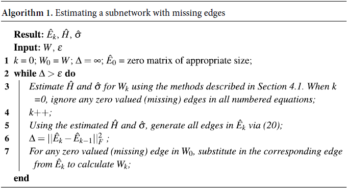
After this estimation process completes, we can move back from estimation to generation. The upshot of this entire process is that given one weighted network with missing edges, we can estimate both the adjacency network generating process and the edge weight generating process. This information can serve to generate new weighted networks with missing edges, using (22) to get a synthetic edge weight network, and using the estimated SBM-type parameters based on the observed adjacency network to generate a synthetic adjacency network. Finally, take the Hadamard product of these two matrices to generate a synthetic network where the distributions for each edge weight match the estimated distribution in the original network, including treating 0 as a missing edge.
7.2 Noisy edge weights
Our estimation method appears to work even when a dense network is not generated as an
 $H$
-Normal NSM. Rearranging (9),
 \begin{equation*}W_{uv} = G^{-1}\!\left (\Phi _1\!\left (\frac {1}{\sqrt {1+\sigma ^2}} \Phi _1^{-1}(H(\Psi _u, \Psi _v))+ \frac {\sigma }{\sqrt {1+\sigma ^2}} \varepsilon _{uv}\right )\right ).\end{equation*}
If
 $G$
is a distribution with a maximum, that means no edge weight can exceed that maximum. However, if we include another term
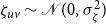 $\zeta _{uv} \sim \mathcal{N}(0, \sigma _{\zeta }^2)$
into
 \begin{equation*}W_{uv} = G^{-1}\!\left (\Phi _1\!\left (\frac {1}{\sqrt {1+\sigma ^2}} \Phi _1^{-1}(H(\Psi _u, \Psi _v))+ \frac {\sigma }{\sqrt {1+\sigma ^2}} \varepsilon _{uv}\right )\right ) + \zeta _{uv},\end{equation*}
then, if
 $\sigma _{\zeta }^2 \gt 0$
, each edge weight is distributed over
 $\mathbb{R}$
. As can be seen in Appendix E.4 of Leinwand & Pipiras (Reference Leinwand and Pipiras2022), the estimation procedure still captures the underlying network dynamics in this case, although the estimates degrade as
 $\sigma _{\zeta }^2$
increases.
8. Simulations
For each simulation, we include a description and a figure showing the original network and the estimated underlying network, where the clustering choice is the estimated measure
 $L$
maximizing clustering using the algorithms presented in Appendix D of Leinwand & Pipiras (Reference Leinwand and Pipiras2022). Additional simulations and results are presented in Appendix E.
8.1 Varying
$\sigma$

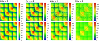
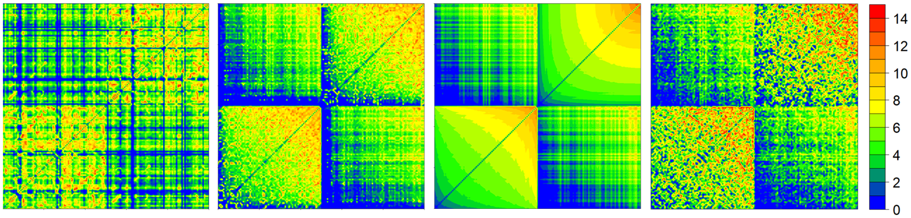
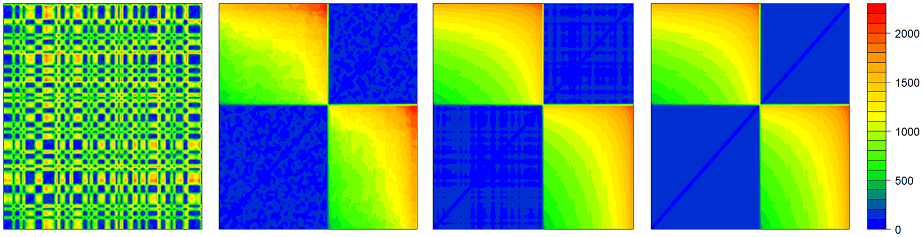
Figure 3 depicts variations on and estimates of an underlying network with 4 communities of 37 nodes each. In plot A, the network is displayed with
 $\sigma = 0$
. Within community edges are drawn from a uniform distribution with a maximum of 150, while between community edges are drawn from a uniform distribution with a maximum of 100. Node sociability parameters for both communities are equally spaced, ranging from 0.05 to 0.95 in increments of 0.025. The
 $H$
-function is the same as that used for the rightmost plot in Figure 2, though since the between community edges have negative association, the inputs to that
 $H$
-function are
 $1 - \Psi _u$
and
 $1 - \Psi _v$
. This network is ordered so one can visually discern communities and connectivity patterns. Even so, the first step is to estimate community structure, as node ordering does not impact the community detection algorithm. The resulting estimated network is shown below the original and looks very similar to the original network.
A single
 $H$
-Normal NSM with different
 $\sigma$
values. The estimate of each network is shown below the original network being estimated.
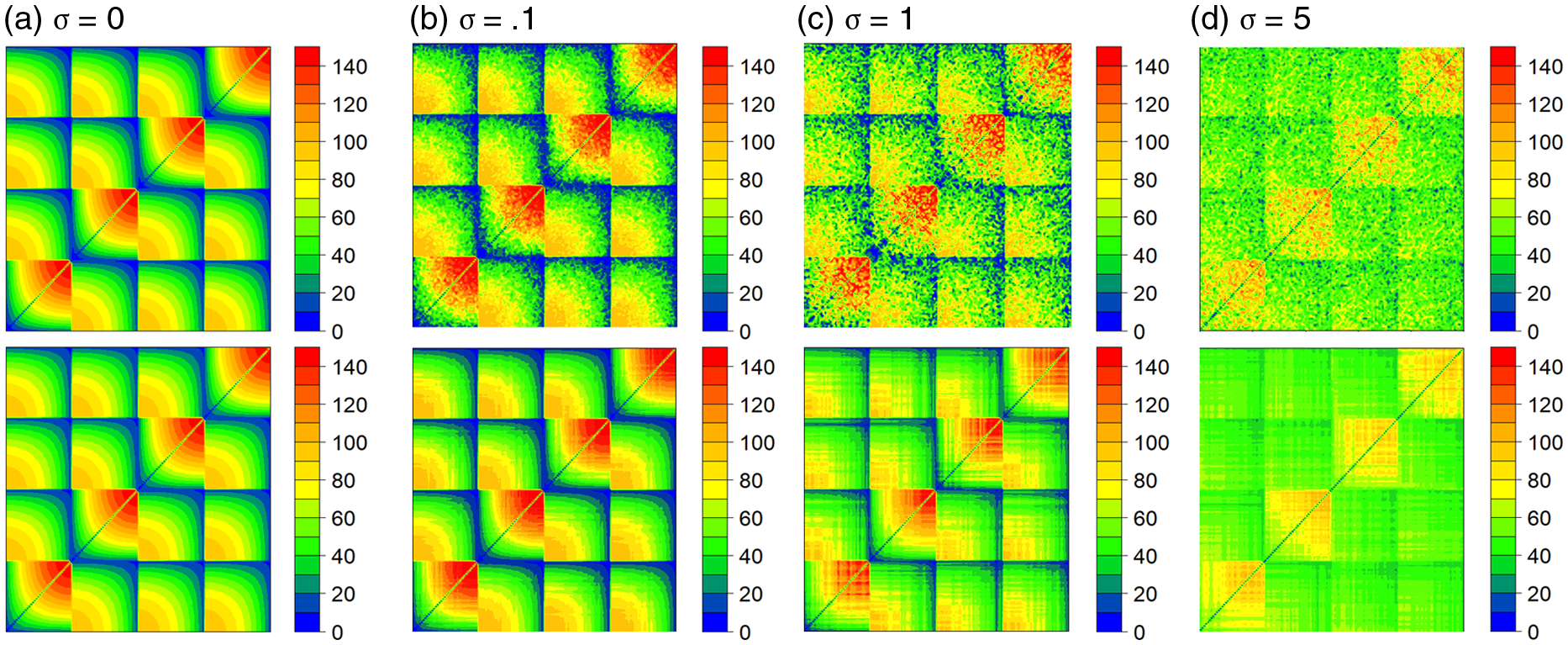
Where plot A uses (9) with
 $\sigma = 0$
, plot B uses
 $\sigma =.1$
leaving the network looking smudged. The estimate looks like a smoothed version of the actual observed network, albeit somewhat “blurrier” than the underlying network seen in plot A. This performance degradation with increasing
 $\sigma$
is to be expected. In plot C,
 $\sigma =1$
, and the fidelity of the estimated network continues to degrade. In plot D, where
 $\sigma = 5$
, there is far less apparent degree correction. Instead, the distribution of within community edge weights appears to stochastically dominate that of the between community edge weights. In this case, the observed network actually resembles a Weighted Stochastic Block Model. The estimates are shrunk towards the median of the observed edge weights in each subnetwork, and exhibit some moderate degree correction.
Plot A would look identical with repeated sampling, but the other three plots would vary randomly by construction. To account for this randomness, we generated 300 networks using the same construction as in Figure 3, with 25 networks for each of 12 conditions using the following parameter combinations. Half of the networks had 148 nodes (37 nodes in each of 4 communities), while the other half had 292 nodes (73 nodes in each of 4 communities), with evenly spaced sociability parameters ranging between 0.05 to 0.95. In each network size, 25 networks were generated with
 $\sigma$
taking each of the values 0.1, 0.5, 1, 2, 3, and 5.
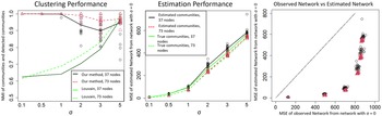
Rather than visually inspecting all 300 networks and their estimates, we provide estimates of clustering performance in Figure 4. First, we plot the average Normalized Mutual Information (NMI) between the true communities and the estimated community assignments based on our proposed methodology, as well as when using Louvain clustering (Blondel et al., Reference Blondel, Guillaume, Lambiotte and Lefebvre2008). For our method, we also display NMI values for each individual network, using black circles to represent networks with 148 nodes, and red triangles to represent networks with 292 nodes. As to be expected, our method performs better when
 $\sigma$
is smaller (nearly perfectly when
 $\sigma \le 1$
), and when there are more nodes per community. What is perhaps more interesting is that while our method far outperforms Louvain clustering when
 $\sigma$
is small to moderate, when
 $\sigma =5$
, the network is actually clustered more accurately using Louvain clustering. This observation, paired with plot D from Figure 3 yields an interesting insight. In the special case when
 $\sigma = \infty$
, if the distribution of edge weights between communities is dominated by the distribution of edge weights within communities, our proposed model effectively becomes a Weighted Stochastic Block Model.
On the left, NMI of true communities and estimated communities for different values of
 $\sigma$
. In the middle, the average squared distance between edges in the estimated network to edges in the underlying network with
 $\sigma =$
0. On the right, the average squared distance from edges in the underlying network with
 $\sigma =$
0 for the edges in the observed network and edges in the resulting estimate.
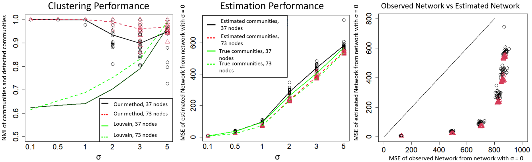
The middle plot of Figure 4 shows the estimation error using both the estimated communities using our method, and if we used the true communities. We display individual network values only using estimated communities, using the same symbols as in the left plot. In this case, the error is the average squared deviation in edge weight from the estimated network to the underlying network with
 $\sigma =0$
. Unsurprisingly, the error increases with
 $\sigma$
. Surprisingly, the number of nodes per community does not appear to have a huge impact on the error. Perhaps even more surprisingly, the estimates using the estimated communities do not appear to perform much worse than those using the true communities.
Finally, the right plot shows the average squared “error” in the observed network against the average squared error in the estimated network. In all cases, the estimates are closer in mean squared deviation to the underlying network than the observed networks, since all coordinates lie below the 45 degree line. However, noting that the y-axis in the middle plot represents the same information as in the right plot, this advantage wanes as
 $\sigma$
increases, particularly when it exceeds 1, the point where the SC pattern has as much influence as the
 $\varepsilon$
value.
Taken together, these results indicate there is a regime where the estimation techniques described in this paper appear to overwhelmingly succeed, and that for
 $0 \le \sigma \le 1$
, the network is likely in that regime. Determining when our proposed approach is appropriate merits further investigation. Though in real settings, the true value of
 $\sigma$
is unknown (and may depend on the subnetwork), it can be estimated. Under certain assumptions, the estimate of
 $\sigma$
can serve as a measure of whether the approach appears to be succeeding. The following example demonstrates an alternative approach using the method from Section 4.3.
8.2 Disassortative network with spurious patterns
Figure 5 introduces several changes. First, the communities are disassortative, as between community edges are larger than within community edges. Second, the within community edge weights are i.i.d. Third, the between community edge weights are generated using randomly generated Gamma parameters for each node, and using those as inputs into a negative binomial distribution. This is not generated as an
 $H$
-Normal NSM, yet we still use our estimation procedure. Fourth, the nodes are not ordered. If the true community orderings are not known a priori, a network may look like the left plot of Figure 5. Following estimation, the communities are clustered correctly, and the between community estimate broadly looks smoother than the original network. The initial estimated network appears to amplify spurious structure in the within community edges, giving some order to the pure randomness seen in the original network. Utilizing the procedure discussed in Section 4.3, within community edges for subnetworks with spurious patterns are replaced by the median value of that subnetwork’s edge weights.
Network with spurious pattern of within community edges. From left to right: original, reordered, initial estimate, final estimate.
8.3 Missing edges
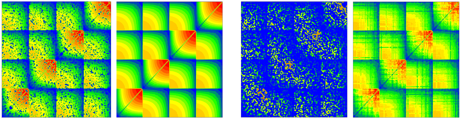
Figure 6 shows the network in Figure 3 after deleting many edges at random, along with the final estimated networks using the procedure discussed in Section 7.1. The communities are estimated for the network with 20% of the edges missing, but are assumed to be known for the network with 75% of edges missing. Even accounting for this, as one might expect, the reconstruction is more successful with fewer missing edges.
Networks with missing edges. Left: network with 20% of edges deleted and its estimate. Right: network with 75% of edges deleted and its estimate.
9. Applications
In this section, we show how the methods described in this paper work on real data where the ground truth clusterings are unknown. In this case, we will show the original network, the network reordered by community then within community degree, and then show the estimated network.
9.1 Brain networks
Figure 1, which has already been discussed in Section 1, shows a preprocessed DTI scan from the ADNI database (
http://adni.loni.usc.edu
). As in Leinwand et al. (Reference Leinwand, Wu and Pipiras2020), for this scan, the cortical surface has been parcellated into the 148 regions of the Destrieux Atlas using FreeSurfer on the T1-weighted MRI scan. Then probabilistic fiber tractography was applied on DWI and T1-weighted images using FSL software library to obtain a 148
 $\times$
148 matrix. Each entry in the matrix is the log of the count of white matter fibers connecting two brain regions.
In contrast to the structural brain network discussed above, Figures 7 and 8 show the functional brain networks of subject IDs 293 and 108 from Brown et al. (Reference Brown, Rudie, Bandrowski, Van Horn and Bookheimer2012), two preprocessed fMRI scans from the ADHD-200 sample. Both networks come from females, where one is age 10.73 and typically developing, and the other is age 10.81 with ADHD. Both are processed using the Athena pipeline resulting in 190 regions. More details about preprocessing can be found at http://umcd.humanconnectomeproject.org .
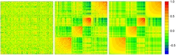
ADHD brain network.
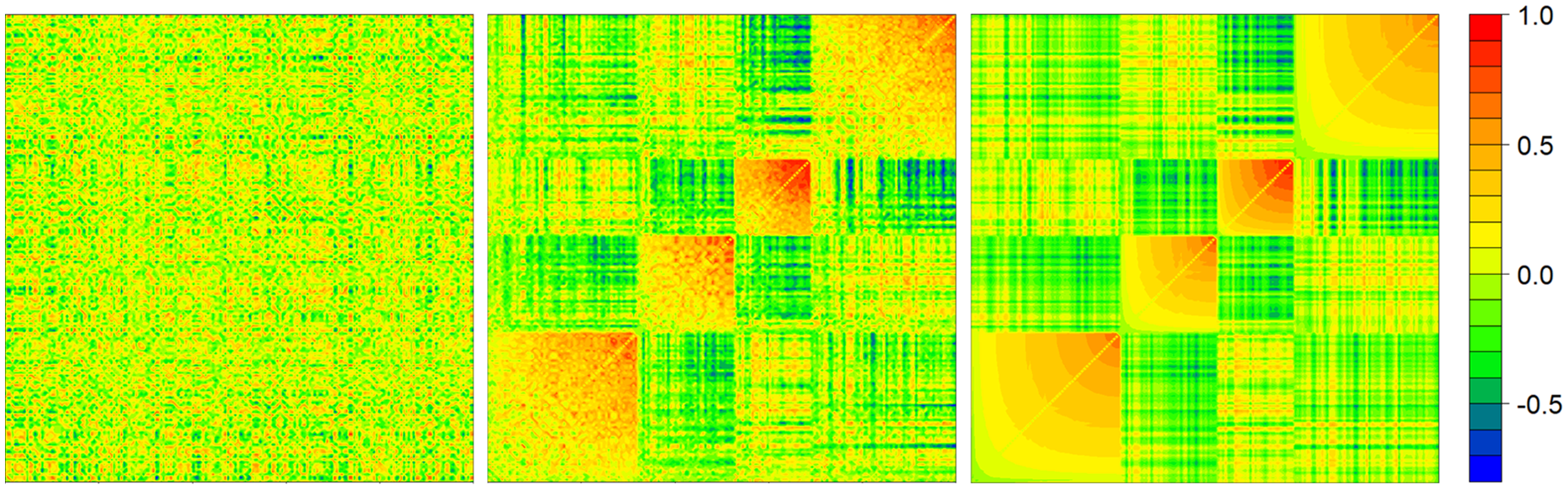
Control brain network.
The most obvious difference between the results is the ADHD network is split into 4 communities, while the typical network breaks into 5 communities. Looking at the typical network, we see clearer negative associations between communities than in the ADHD network, particularly accounting for the slightly different axes. The estimate of both networks shows some “plaid” looking patterns, as opposed to colors monotonically changing in one direction, which indicates the ordering of
 $\Psi$
values within communities may not be the same as the ordering of
 $\Psi$
values between communities. More defined communities and greater negative association patterns in the typical scan would appear to support the hypothesis that ADHD subjects exhibit less modular brain organizations than typical subjects.
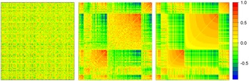
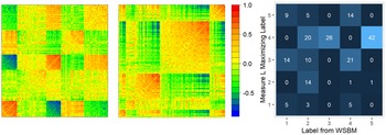
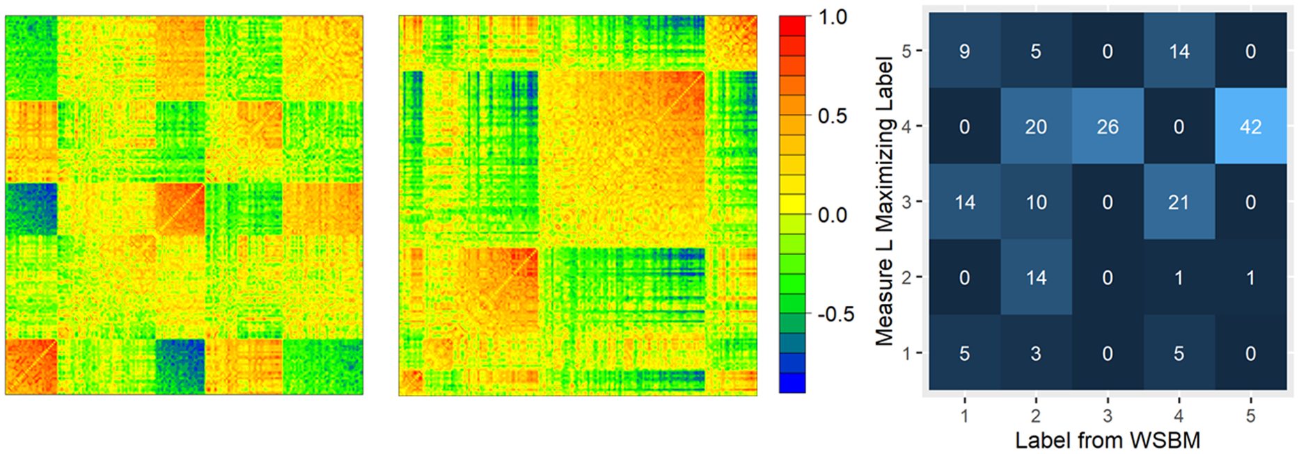
Figure 9 shows the control network rearranged and estimated based on WSBM community detection, using the Matlab package accompanying (Aicher et al. Reference Aicher, Jacobs and Clauset2013, Reference Aicher, Jacobs and Clauset2015). Our model does require prespecification of the number of communities nor the distribution of edge weights within or between communities, but for the sake of comparison, we instruct their package to mimic the structure of our results as best as possible, segmenting the network into 5 communities, ignoring the edge distribution, and assuming the weight distribution is Normal. WSBM appears to cluster nodes such that the induced subnetworks have edge weights confined to a relatively narrow band of values, which gives the impression of more solid colors and fewer gradients in the rearranged matrix. It also produces relatively evenly sized clusters. Using an
 $L$
maximizing algorithm, on the other hand, produces a larger community containing almost half of the nodes. The
 $L$
maximizing communities produce a measure value of 6,580 compared to 3,276 for the WSBM communities. Implementing the estimation methods from Section 4, the mean squared error of the final estimated matrix in Figure 8 is 0.024 compared to 0.033 if using the WSBM estimates. The WSBM communities also yield larger
 $\widehat{\sigma }$
values. This provides evidence that the community detection using the measure
 $L$
is capturing something different than WSBM community detection, and likely a signal more suitable for the estimation methods described in this paper. Further experimentation has shown that WSBM community detection of plot A in Figure 3 does not match the intuitive visual clustering. Functional brain networks may not be organized according to an NSM or LSM, but the presence of detectable negative associations merits further investigation.
From left to right: control brain network reordered by communities estimated using WSBM. The same network reordered by communities estimated using an approximate
 $L$
maximizing algorithm. The confusion matrix of node labels between these community estimates (note that label values do not reflect ordering).
9.2 State-to-state migration “affinity”
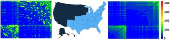
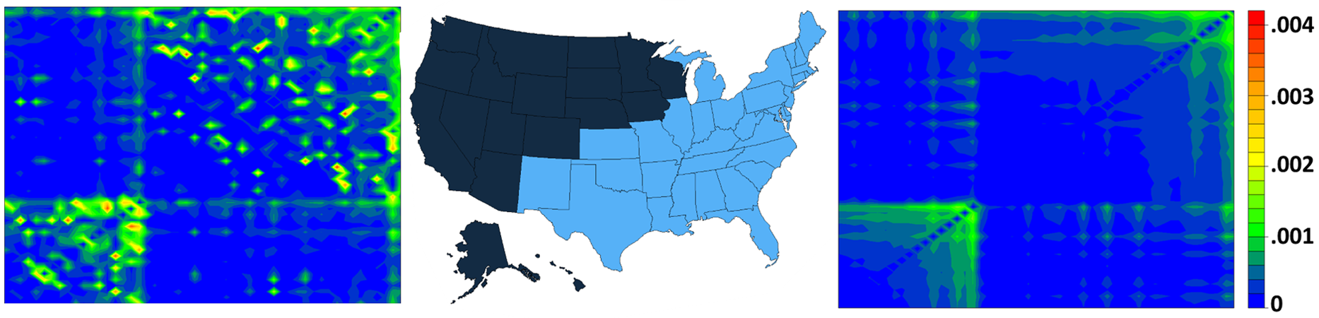
Taking the state-to-state migration flows data from the 2017 American Community Survey 1-Year Estimates and dividing each cell in that table by the outgoing state’s total outflows gives a transition probability matrix for those people who left their state in 2017. For the network shown in Figure 10, this transition probability matrix is added to its transpose to get a symmetric matrix. This final network ignores the direction of greater inflows or outflows, but instead represents the “affinity” between the two states in question. The results show geographic communities which appear to give a reasonable segmentation based on geography. The estimated network displays positively associated within community dynamics, indicating both homophily and degree correction. However, the within community
 $\widehat{\sigma }$
estimates are relatively large for this network, so these estimates have a relatively narrow range. This may be due to small subnetwork size, but also because some of the largest values lie in the interior of the subnetworks, rather than on the frontier.
2017 state-to-state migration.
10. Conclusions
We have introduced new models for dense weighted networks, wherein edge weights depend on node sociabilities and community memberships. The development of these models spurred estimation techniques for networks of this kind. With minor modifications, these estimation techniques appear to be applicable to an even broader class of networks than those introduced in this paper. Furthermore, one can use the results from (21) as a gauge of whether the described estimation process is appropriate for a particular network.
One potential consideration for future work is determining whether
 $\Psi$
values should be estimated at the global or local level. In a case where each node’s
 $\Psi$
value is globally consistent, estimating it across the whole network would be preferred to estimating several local estimates. However, given potentially different
 $H$
-functions across different subnetworks, pooling this information is not necessarily straightforward. Similarly, a different kind of information pooling may also play an important role for modeling the dynamics of a given network observed repeatedly over time. The introduced models may also lend themselves to extensions for more generalized forms of graphs such as multilayer networks or—following up on Appendix F of Leinwand & Pipiras (Reference Leinwand and Pipiras2022)—hypergraphs.
Competing interests
None.
Data availability statement
Code to support the findings of this study is available as supplementary information. Data used in this study are available from the ADNI database (http://adni.loni.usc.edu), the Human Connectome Project (http://umcd.humanconnectomeproject.org), and the American Community Survey (https://www.census.gov/data/tables/time-series/demo/geographic-mobility/state-to-state-migration.html).
Supplementary materials
For supplementary material for this article, please visit http://doi.org/10.1017/nws.2022.23