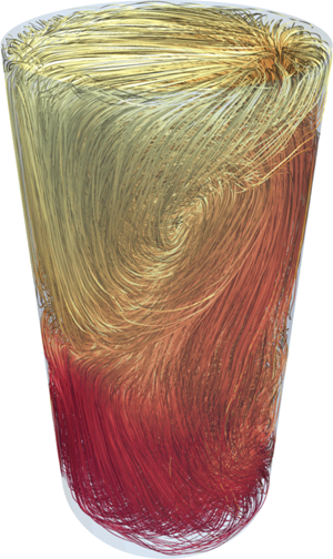



1. Introduction
Thermal convection, a fluid motion driven by temperature gradients, is ubiquitous in nature and technological processes. Examples are found in geophysics and oceanography (Marshall & Schott Reference Marshall and Schott1999), convection in the outer liquid core of the Earth (Christensen & Aubert Reference Christensen and Aubert2006) and heat exchange processes in nuclear reactors (Salavy et al. Reference Salavy, Boccaccini, Lässer, Meyder, Neuberger, Poitevin, Rampal, Rigal, Zmitko and Aiello2007) to mention a few. In several of these examples, the thermal convection processes occur at a low Prandtl number
 \begin{equation} Pr = \frac{\nu_f}{\kappa_f} \lesssim {O}(10^{-2}), \end{equation}
which comprises working fluids such as liquid metals or semiconductor melts. Here,  $\nu _f$ and
 $\kappa _f$ stand for the kinematic viscosity and thermal diffusivity of the fluid, respectively. The idealized and most frequently studied system of thermally driven turbulence is that of turbulent Rayleigh–Bénard convection (RBC), where a fluid confined between two thermally conducting horizontal plates is heated uniformly from below and cooled from above (Ahlers, Grossmann & Lohse Reference Ahlers, Grossmann and Lohse2009; Chillà & Schumacher Reference Chillà and Schumacher2012). Comprehensive studies of different aspects of RBC over the past decades were mainly focussed on working fluids with larger Prandtl numbers and the low-Prandtl-number case has been much less studied either numerically, experimentally or theoretically due to several difficulties. For example, for low-
 $Pr$ convection the nonlinearity that leads to inertial fluid motion is stronger and hence the RBC system develops stronger turbulent fluctuations compared to a large-
 $Pr$ case at the same outer temperature difference. This requires finer computational meshes for direct numerical simulations.
Liquid metals are opaque and thus flow visualization and measurement of the fluid velocity and temperature are challenging (Takeshita et al. Reference Takeshita, Segawa, Glazier and Sano1996; Cioni, Ciliberto & Sommeria Reference Cioni, Ciliberto and Sommeria1997; Horanyi, Krebs & Müller Reference Horanyi, Krebs and Müller1999). In a recent experimental study, Zürner et al. (Reference Zürner, Schindler, Vogt, Eckert and Schumacher2019) employed combined measurements of velocity components and temperature in a cylindrical cell using liquid metal alloy GaInSn at  $Pr=0.029$. In their series of experiments they reconstructed and characterized the coherent large-scale circulation (LSC) in the cell and determined the turbulent heat transfer from the volume flux of the cooling water through the top plate and the temperature difference. In liquid metal convection experiments, the convection cell is bounded by copper plates whose thermal conductivity differs by a factor of 10 only to that of the working fluid (see also table 1 for example). This can alter the uniformity of temperature distribution at the plate–fluid interfaces and consequently affect the heat transfer, as also discussed by Horanyi et al. (Reference Horanyi, Krebs and Müller1999) for sodium experiments (where the conductivity ratio is even smaller) and Cioni et al. (Reference Cioni, Ciliberto and Sommeria1997) for measurements in liquid mercury. In laboratory experiments with liquid metals, the thermal boundary conditions (BCs) at the top and bottom will thus deviate from an ideal fixed-temperature case and rather should be considered as some mixture of both, prescribed temperature and prescribed heat flux.
Examples for the material parameters of the plates and the working fluids. The values for air are taken at normal pressure and at  $20\,^{\circ }\textrm {C}$. The values for GaInSn are taken at
 $26\,^{\circ }\textrm {C}$ following Plevachuk et al. (Reference Plevachuk, Sklyarchuk, Eckert, Gerbeth and Novakovic2014). The thermal conductivity of copper at the same temperature is taken from Hust & Lanford (Reference Hust and Lanford1984). All values depend sensitively on temperature. While the thermal diffusivity ratios
 $\kappa _{Cu}/\kappa _{GaInSn}\approx 10$ and
 $\kappa _{Cu}/\kappa _{air}\approx 5.2$, the thermal conductivity ratios
 $\lambda _{Cu}/\lambda _{GaInSn}\approx 15$ and
 $\lambda _{Cu}/\lambda _{air}\approx 14\,800$.

This sets the main motivation for the present numerical study in which we want to address the impact of 3 different thermal boundary conditions on three-dimensional convective turbulence with a particular emphasis on the low-Prandtl-number case. In detail, we discuss a set of 9 direct numerical simulations (DNS), 3 runs for convection in air at a Rayleigh number  $Ra= 10^7$ and 6 runs for convection in the liquid metal alloy GaInSn at
 $Ra=10^7$ and
 $10^8$ (parameters will be defined in § 2). Our study compares constant-temperature boundary conditions with constant flux boundary conditions. In both cases one assumes an infinitely thin plate at the top and bottom. The third set of runs, the conjugate heat transfer case, contains finitely thick copper plates at the bottom and top as in reality. This requires a match of temperatures and heat fluxes at the fluid–plate interfaces. We compare several statistical parameters, such as mean and fluctuation profiles of selected quantities and the fine-scale statistics. The latter includes distributions of locally defined boundary layer thicknesses. Our study focusses on the thermal conditions at the bottom and top plates.
For the conjugate heat transfer set-up, rigorous bounds on the turbulent heat transfer have been derived by Wittenberg (Reference Wittenberg2010). He showed that the prefactor that enters the upper bound  $Nu\le C Ra^{1/3}$ depends on both, the ratio of plate thickness to layer height as well as the ratio of thermal conductivities. Here, Nusselt number
 $Nu$ is a dimensionless measure of the heat transfer.
The sidewalls are considered as adiabatic (or thermally insulated) which implies that the supplied heat has to pass through the working fluid from the bottom to the top. Non-ideal sidewall effects on the heat transport and flow properties have been studied in detail numerically by Verzicco (Reference Verzicco2002), Stevens, Lohse & Verzicco (Reference Stevens, Lohse and Verzicco2014) and more recently by Wan et al. (Reference Wan, Wei, Verzicco, Lohse, Ahlers and Stevens2019). They showed that once the sidewalls have a finite thickness (and thus thermal conductivity and heat capacity have to be included) the large-scale flow and thus the turbulent heat transfer are affected. Our work has a different focus and extends existing studies on the influence of different thermal boundary conditions on turbulent convection to low Prandtl numbers where experiments are challenging, as motivated above. We will set up the cases in our DNS such that they are directly comparable which is challenging in an experiment as one cannot control the interface between solid plate and working fluid, in particular for the liquid metal case.
The influence of the thermal properties of the plate on the primary instability of the conductive state has been studied in works of Sparrow, Goldstein & Jonsson (Reference Sparrow, Goldstein and Jonsson1964), Hurle, Jakeman & Pike (Reference Hurle, Jakeman and Pike1967), Chapman & Proctor (Reference Chapman and Proctor1980) and Verzicco (Reference Verzicco2004). Specifically, the work of Hurle et al. (Reference Hurle, Jakeman and Pike1967) highlights the long-wavelength nature of the primary instability for the fixed flux case. Detailed experimental studies of the coupling between turbulent flow and plate conduction processes were for example reported by Chillà et al. (Reference Chillà, Rastello, Chaumat and Castaing2004) in cylindrical and by Huang et al. (Reference Huang, Wang, Xi and Xia2015) in rectangular cells. Verzicco (Reference Verzicco2004) performed comprehensive numerical studies in a cylinder of  $\varGamma =D/H=1/2$ at
 $Pr=0.7$ which were dedicated to the influence of the finite conductivity of the top and bottom plates on the turbulent heat transport (
 $D$ is the diameter and
 $H$ is the height of the cell). He suggested that the effects of the plates can be governed by the ratio of the thermal resistance of the fluid layer to that of the plates, and developed an electrical circuit analogue that quantified the resulting effect on the Nusselt number
 $Nu$, the dimensionless measure of turbulent heat transfer. The model was confirmed later in experiments by Brown et al. (Reference Brown, Nikolaenko, Funfschilling and Ahlers2005) who investigated the effect of conjugate heat exchange on convection in cylinders with various aspect ratios, all filled with water. The outcome was that plates of finite conductivity diminish the global heat transport. Verzicco & Sreenivasan (Reference Verzicco and Sreenivasan2008) combined in their DNS at high
 $Ra$ a constant flux boundary condition at the bottom with a constant-temperature boundary condition at the top in a cell at
 $\varGamma =1/2$ at
 $Pr=0.7$. They found that the Nusselt number
 $Nu$ for
 $Ra>10^9$ is slightly reduced for this configuration compared to that with isothermal BCs at both plates and thus closer to experimental data. A constant flux BC inhibits thermal plume growth. Two-dimensional DNS at
 $Pr=1$ by Johnston & Doering (Reference Johnston and Doering2009) showed that the global heat transfer law is insensitive to the plate conductivity for
 $Ra\gtrsim 10^7$ and resulted in a
 $Nu\sim Ra^{2/7}$ law for both, fixed-temperature and fixed flux BCs. This implies that the Rayleigh numbers should not be too small for such an analysis which is a challenge for the low-Prandtl-number studies conducted here.
The outline of the paper is as follows. In the next section, we present the model equations, the numerical method and the 9 different DNS data sets. Section 3 discusses the global heat and momentum transfer. In § 4, we present our findings for the statistics of temperature and velocity fluctuations. Section 5 presents a detailed analysis of the boundary layers. Finally, we summarize our findings and give a brief outlook.
2. Simulation model
2.1. Equations and parameters
We solve the three-dimensional equations of motion of thermal convection with the Boussinesq approximation. We consider a fluid of depth  $H$, with a kinematic viscosity
 $\nu _f$ and a thermal diffusivity
 $\kappa _f$ at constant mass density
 $\rho _f$. The specific heat at constant pressure
 $c_{p,f}$ and the thermal conductivity
 $\lambda _{f}=\rho _f c_{p,f}\kappa _f$ are given. The equations for non-dimensional fluid velocity
 ${\boldsymbol {u}}({\boldsymbol {x}},t)$ and fluid temperature
 $T({\boldsymbol {x}},t)$ are given by
 \begin{gather} \boldsymbol{\nabla}\boldsymbol{\cdot}\boldsymbol{u} = 0, \end{gather}
 \begin{gather}\frac{\partial \boldsymbol{u}}{\partial t}+(\boldsymbol{u}\boldsymbol{\cdot}\boldsymbol{\nabla})\boldsymbol{u}=-\boldsymbol{\nabla} p+\sqrt{\frac{Pr}{Ra}}\nabla^{2} \boldsymbol{u}+T \boldsymbol{e}_z, \end{gather}
 \begin{gather}\frac{\partial T}{\partial t}+(\boldsymbol{u}\boldsymbol{\cdot}\boldsymbol{\nabla}){T}=\frac{1}{\sqrt{Ra Pr}}\nabla^{2}T, \end{gather}
with the unit vector in vertical direction  $\boldsymbol {e}_z$. The kinematic pressure field is denoted by
 $p({\boldsymbol {x}},t)$. The equations (2.1)–(2.3) are made dimensionless by the fluid depth
 $H$, the free-fall velocity
 $U_f=(g\alpha \tilde {\varTheta } H)^{1/2}$, and the characteristic temperature scale
 $\tilde {\varTheta }$ for the specific thermal boundary conditions (details are given below). Here,
 $\alpha$ is the thermal expansion coefficient and
 $g$ is the acceleration due to gravity. For clarity in our notation, we set a tilde for the temperature scale with a physical dimension.
For turbulent RBC there are three main input parameters which control the system; the aspect ratio  $\varGamma$ which is fixed to 1/2 here, the Prandtl number
 $Pr$ and the Rayleigh number
 $Ra$. The specific definition of
 $Ra$, which quantifies the strength of thermal driving of the turbulence, depends on the prescribed boundary conditions, and is given by
 \begin{equation} Ra=\frac{\alpha g H^3}{\nu_f \kappa_f} \tilde{\varTheta}. \end{equation}
In all three cases studied here, we consider the equilibrium state of pure conductive heat transfer as the initial condition. It takes the form
 \begin{equation} T= 1 - z, \quad \textrm{for}\ 0 < z < 1. \end{equation}
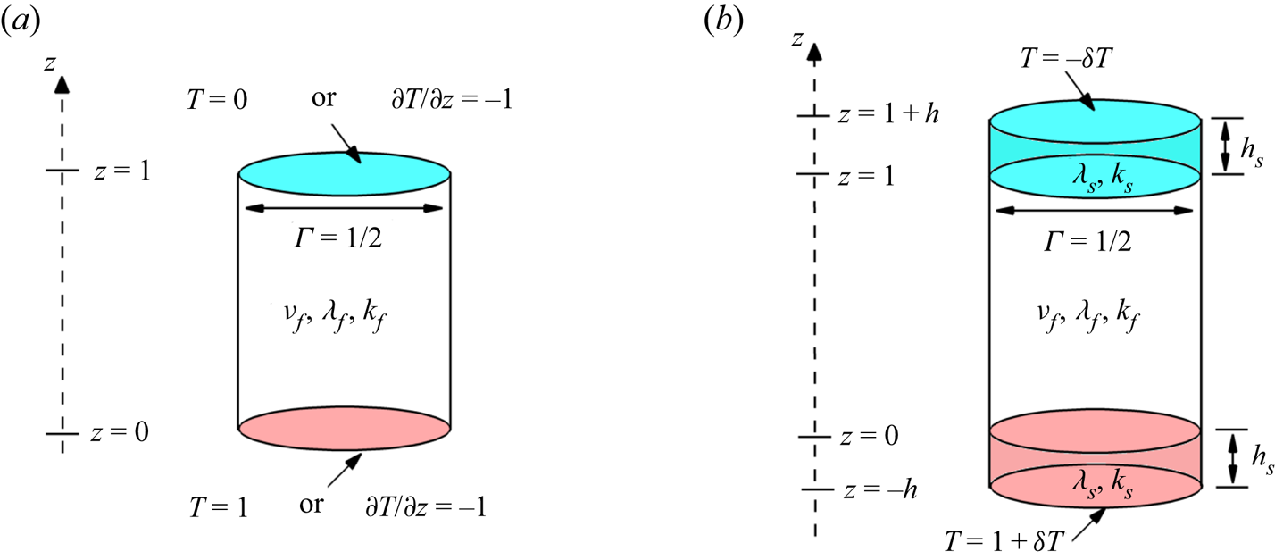
The specification of (2.1)–(2.3) is completed once the conditions at all boundaries are specified. We either impose the thermal boundary conditions directly at the top and bottom interfaces of the fluid volume as seen in figure 1(a) or at the bottom/top of the solid plates as sketched in figure 1(b) for the conjugate heat transfer case. This is specified in the following in detail as well as the other remaining boundary conditions.
A schematic showing different boundary conditions and parameters in Rayleigh–Bénard convection in a cylindrical cell of aspect ratio  $\varGamma =D/H=1/2$. The working fluid has a constant kinematic viscosity (
 $\nu _f$), thermal conductivity (
 $\lambda _f$) and thermal diffusivity (
 $\kappa _f$).
 $(a)$ The constant-temperature (Dirichlet BC) or constant heat flux is imposed at the lower and upper boundaries.
 $(b)$ The cylinder cell is bounded by conductive plates having a thickness of
 $h_s$, thermal conductivity (
 $\lambda _s$) and thermal diffusivity (
 $\kappa _s$) with constant temperature at the boundaries. Values at the vertical coordinate axes and for the temperature or its derivative are non-dimensional.

2.2. Constant temperature and heat flux at bottom and top plates
The typical and most frequently studied thermal BC at the bottom and top interfaces is that of a constant temperature, which is known as the Dirichlet boundary condition. These Dirichlet BCs introduce a temperature scale  $\tilde {\varTheta } = \Delta \tilde {T}$ which is the temperature difference between bottom hot and top cold plates. The non-dimensional form of these thermal BCs is
 \begin{equation} T \mid_{z=0}= 1 \quad\textrm{and}\quad T \mid_{z=1}= 0. \end{equation}
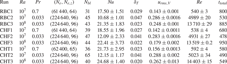
Consequently, the Rayleigh number follows as  $Ra=\alpha g \Delta \tilde {T} H^3/\nu _f \kappa _f$, which we will be called the RBC case in the following. A detailed overview of the simulations can be found in table 2.
Parameters of the different spectral element simulations for Rayleigh numbers  $Ra=10^7$ and
 $10^8$ with the convection cell of aspect ratio
 $\varGamma =1/2$. We list additionally the Prandtl number
 $Pr$, the total number of spectral elements
 $N_{e}$, the number of spectral elements in the vertical direction
 $N_{e,z}$ and the number of grid planes inside the thermal boundary layer. Furthermore, the Nusselt number
 $Nu$ (see § 3 for definition), the thermal boundary layer thickness
 $\delta _T=1/(2 Nu)$, the root mean square velocity taken in the whole fluid volume with respect to all three velocity components
 $u_{{rms},V}$, the Reynolds number
 $Re$, and the total integration time
 $t_{total}$ in units of the free-fall time
 $t_f=H/U_f$ are listed. This is the time interval for which the flow is in a statistically stationary regime and the analysis is conducted on the basis of three-dimensional snapshots.

The second choice is to impose constant vertical heat flux (CHF) at the top and bottom boundaries,  $\partial \tilde {T}/ \partial \tilde {z}=-|\beta |$, which is known as the Neumann boundary condition. In this limit, the dimensionless thermal BCs are
 \begin{equation} \frac{\partial T}{\partial z}= -1 \quad \text{on}\ z =0 \ \textrm{and}\ z =1. \end{equation}
The corresponding temperature scale is now  $\tilde {\varTheta }=|\beta | H$. Therefore, the typical length, velocity and temperature scales are given by,
 $H, \sqrt {\alpha g |\beta | H^2}$ and
 $|\beta | H$, respectively. The Rayleigh number in this case (
 $Ra_q$) and its relation to the Rayleigh number for the RBC case are given by
 \begin{equation} Ra_q = \frac{\alpha g |\beta| H^4}{\nu_f \kappa_f}, \quad Ra_q=Ra\frac{|\beta| H}{\Delta \tilde{T}}= Ra Nu , \end{equation}
as discussed by Otero et al. (Reference Otero, Wittenberg, Worthing and Doering2002), Verzicco & Sreenivasan (Reference Verzicco and Sreenivasan2008) and Johnston & Doering (Reference Johnston and Doering2009). We denote this second case by CHF (see again table 2). Consequently, one can find  $\boldsymbol {u}_{CHF}= \sqrt {Nu}\,\boldsymbol {u}_{RBC}$ and
 $T_{CHF}=T_{RBC} Nu$. Here,
 $Nu$ is the Nusselt number, the dimensionless measure of turbulent heat transfer which will be defined in § 3.
2.3. Fluid bounded by finitely thick plates at bottom and top
In order to study the boundary layer structure with more realistic conditions and get as close as possible to laboratory set-up (see e.g. Verzicco & Camussi Reference Verzicco and Camussi2003; Zürner et al. Reference Zürner, Schindler, Vogt, Eckert and Schumacher2019), we also studied the fluid bounded by two finitely thick copper plates from above and below. Now Dirichlet BCs are applied at the top of the upper plate and the bottom of the lower plate, as shown in figure 1(b). The solid plates have the same thickness  $h_s=0.2H$ for the present case with a thermal diffusivity
 $\kappa _s$ and a thermal conductivity
 $\lambda _s=\rho _s c_{p,s}\kappa _s$. For the following, it is more convenient to define the ratio of solid-to-fluid thickness as
 \begin{equation} h=\frac{h_s}{H}. \end{equation}
In this case, the heat conduction equations in the solid parts,  $-h< z< 0$ and
 $1<z<1+h$, for the temperature
 $T_s$ have to be coupled to the advection–diffusion equation (2.3) in the fluid domain ,
 $0 < z < 1$. This configuration is denoted as the conjugated heat transfer (CHT) case. We thus have to solve the additional heat conduction equation in the plates which is given by
 \begin{equation} \frac{\partial \tilde{T}_s}{\partial \tilde{t}}=\kappa_s \tilde{\boldsymbol{\nabla}}^2 \tilde{T}_s \quad\mathrm{for}\ -h_s <z<0 \ \mathrm{and}\ H<z<H+h_s. \end{equation}
Moreover, we require the continuity of temperature and heat flux at the solid–fluid interfaces,
 \begin{gather} \left.\tilde{T}_s\right|_{\tilde{z}=0,H}=\left.\tilde{T}_f\right|_{\tilde{z}=0,H}, \end{gather}
 \begin{gather}\left.\lambda_s\frac{\partial \tilde{T}_s}{\partial \tilde{z}}\right|_{\tilde{z}=0,H}=\lambda_f \left. \frac{\partial \tilde{T}_f}{\partial \tilde{z}}\right|_{\tilde{z}=0,H}. \end{gather}
In the CHT case, we have consequently applied constant temperatures
 \begin{equation} \tilde{T}(\tilde{z}=-h_s) =\tilde{T}(\tilde{z}=0)+\delta \tilde{T} \quad\mathrm{and}\quad \tilde{T}(\tilde{z}=H+h_s) =\tilde{T}(\tilde{z}=H)-\delta \tilde{T}. \end{equation}
The temperature drop across both solid plates varies with  $Pr$ and is adjusted at the boundaries for each case such that the (dimensionless) average temperature (but not locally in time or space)
 $\langle T(z=0)\rangle _{A,t}\approx 1$ and
 $\langle T(z=1)\rangle _{A,t}\approx 0$, respectively, where
 $\langle \cdot \rangle _{A,t}$ stands for an average over the circular cross-section
 $A$ and time
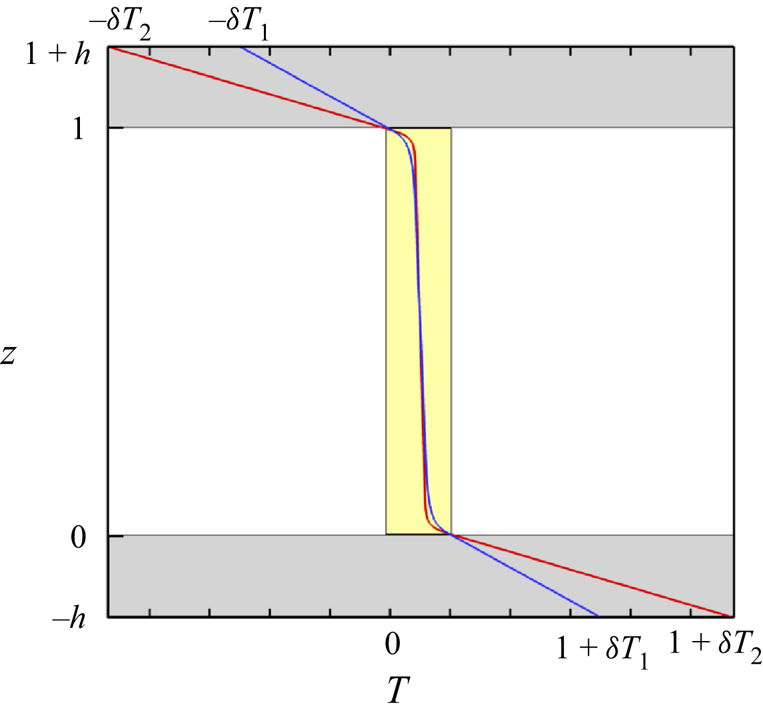
 $t$. When the convection cell is filled with GaInSn, the outer imposed temperature increment is
 $\delta T_1= 2.51$ for
 $Ra=10^7$ and 4.99 for
 $Ra= 10^8$; in case of air it is
 $\delta T_2 = 4.72$ at
 $Ra=10^7$ (see also figure 2). The actual Rayleigh numbers for the cases CHT1, CHT2 and CHT3 thus deviate from the RBC case references by 16 %, 13 % and 9 %, respectively. That means that the solid plates are sensitive to the effective thermal conductivity (
 $\lambda _{eff}= Nu \lambda _s$) rather than the molecular thermal conductivity. The mean temperature profiles for the CHT case in solid–fluid–solid domain are plotted in figure 2 at
 $Ra=10^7$ with
 $Pr=0.7$ and
 $Pr=0.033$. The solid domain is shaded with grey colour and the fluid domain with yellow.
Mean dimensionless temperature profiles in the CHT setting which are compared here for  $Ra=10^7$,
 $\varGamma =1/2$,
 $Pr=0.7$ (red solid line) and
 $Pr=0.033$ (blue solid line). Temperatures have to be adjusted at the outer solid boundaries such that the mean temperatures at the bottom and top interfaces reach
 $\langle T(z=0) \rangle _{A,t}\approx 1$ and
 $\langle T(z=1)\rangle _{A,t}\approx 0$, respectively. The solid plates are shaded in grey. The yellow box indicates the range of the mean temperature profile in the corresponding RBC cases.

In all cases studied here, the computational domain is a cylindrical container of aspect ratio  $\varGamma =1/2$ with
 $x,y \in [-0.25,0.25]$ and
 $z\in [0,1]$. At all walls, no-slip boundary conditions
 $\boldsymbol {u}=0$ for the fluid are applied. The sidewalls are adiabatic, i.e. the normal derivative of the temperature field vanishes (
 ${\partial T}/{\partial \boldsymbol {n}}=0$). Therefore, the RBC, CHF and CHT cases are directly comparable to each other. Similar to the RBC case the reference temperature in the CHT case
 $\tilde {\varTheta }=\Delta \tilde {T}$ is applied across the characteristic scale
 $H$ which results in the same Rayleigh number definition as in the RBC case.
2.4. Numerical method
We numerically solve (2.1)–(2.3) in the fluid domain along with the heat equation (2.10) in both solid plates using the Nek5000 spectral element code optimized and adapted to our problem (Fischer Reference Fischer1997; Deville, Fischer & Mund Reference Deville, Fischer and Mund2002; Scheel, Emran & Schumacher Reference Scheel, Emran and Schumacher2013). The code employs second-order time stepping using a backward difference formula. The entire set of equations is transformed into a weak formulation and discretized with a particular choice of spectral basis functions (Fischer Reference Fischer1997; Deville et al. Reference Deville, Fischer and Mund2002), where Lagrangian interpolation polynomials are expanded into series of Legendre polynomials. In each of the  $N_e$ elements all turbulent fields are expanded by
 $N$th-order polynomials with respect to each spatial direction. In the present study, seventh-order polynomials are taken for all cases such that we have 8 Gauss–Lobatto–Legendre collocation grid points in each direction on each element. The spectral element mesh is non-uniform and becomes finer towards all walls, see e.g. Scheel et al. (Reference Scheel, Emran and Schumacher2013) for a horizontal element arrangement. We list the number of grid points within the thermal boundary layer
 $N_{bl}$ of each case in table 2. For the case of conjugate heat transfer, the number of spectral elements in each plate is
 $N_{e,z}^s=20$ with respect to the vertical direction. The element height is uniform there, the horizontally element shape and thus the resolution corresponds to that in the working fluid volume. We have also verified that our flows are adequately resolved according to the criteria summarized by Scheel et al. (Reference Scheel, Emran and Schumacher2013). Further details on each of the six production runs are summarized in table 2.
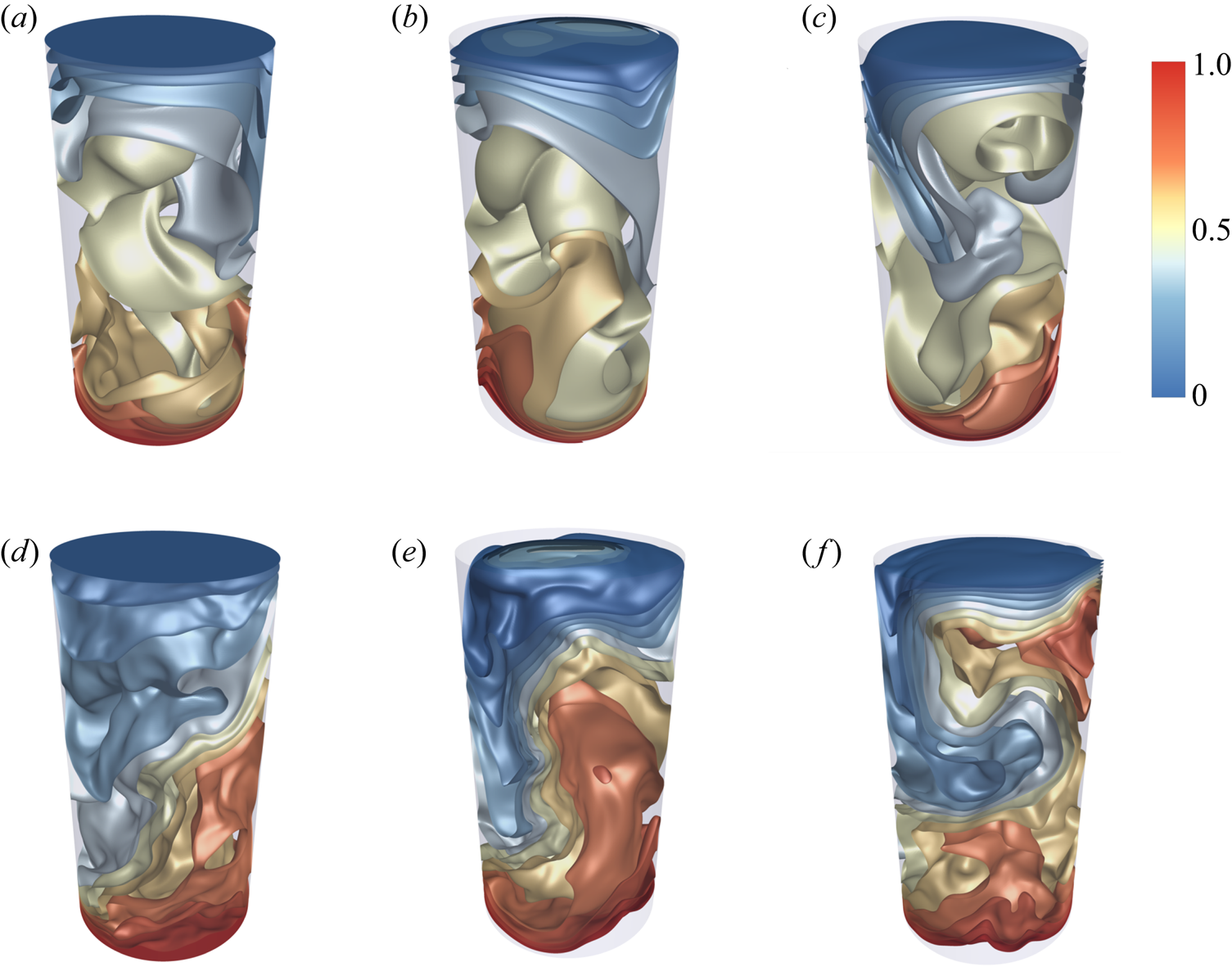
As an example, instantaneous temperature isosurface plots for  $Ra= 10^7$ are shown in figure 3. We plot temperature iso-surfaces of RBC, CHF and CHT for
 $Pr=0.7$ in figure 3(a–c) and for
 $Pr=0.033$ in figure 3(d–f), respectively. At first glance it is clear that the mean flow is similar in all six cases, the size of the isosurfaces changes with
 $Pr$ however. We observe that the surfaces appear less smooth for the case at lower Prandtl number which indicates a higher magnitude of velocity fluctuations. As seen in table 2, the latter are enhanced by a factor of 2 for the liquid metal case in comparison to convection in air. Also visible are the differences of the temperature contours close to the top plate (see figure 3b,e) which suggest differences in the thermal boundary layers.
Instantaneous isosurface plots of the temperature field  $T$ for different boundary conditions, constant-temperature RBC, constant-heat-flux CHF and conjugate heat transfer CHT, all at
 $Ra=10^7$ and
 $\varGamma =1/2$. Panels (a–c) are for
 $Pr=0.7$ and (d–f) for
 $Pr=0.033$.
 $(a)$ Case RBC1.
 $(b)$ Case CHF1.
 $(c)$ Case CHT1.
 $(d)$ Case RBC2.
 $(e)$ Case CHF2.
 $(f)$ Case CHT2. The temperature legend holds for all six panels.

3. Turbulent heat and momentum transport
In thermal convection, the Nusselt number  $Nu$ quantifies the enhancement of vertical heat flux due to (turbulent) fluid motion beyond the diffusive lower bound
 $Nu=1$. The procedure in the standard setting, the RBC case, is to compute the global turbulent heat flux through the cell by
 \begin{equation} Nu=1+\sqrt{RaPr}\langle u_zT\rangle_{V,t}, \end{equation}
where  $\langle \cdot \rangle _{V,t}$ denotes a combined fluid volume and time average. The time average in units of free-fall time is taken over a sequence of statistically independent snapshots. The total time of the statistical analysis
 $t/t_f$ (with the free-fall time
 $t_f=H/U_f$) is listed in table 2. The snapshots are separated by
 $1 t_f$ in RBC, CHF and by
 $0.5 t_f$ in CHT runs. In order to compare the different models, we evaluate the Nusselt numbers directly at the plates. For the cases RBC and CHT, we apply
 \begin{equation} Nu_{RBC}=\left. -\frac{\partial \langle T\rangle_{A,t}}{\partial z} \right|_{z=0,1}=Nu_{CHT}. \end{equation}
When case CHF is studied, the Nusselt number is given by
 \begin{equation} Nu_{CHF}= \frac{\beta}{\Delta \tilde{T}}=\frac{1}{\langle T (z=0)\rangle _{A,t}-\langle T (z=1)\rangle_{A,t}}. \end{equation}
Note that the mean temperature at both plates is now close to 1/2. For run CHF1 we get for example  $\langle T(z=0) \rangle _{A,t}=0.525$ and
 $\langle T(z=0) \rangle _{A,t}=0.473$. The numbers and corresponding error bars are given in table 2. The results are compared with previous numerical and experimental studies; here, we select only those which overlap with our data, and briefly list them here. Our RBC1 simulation is in good agreement with the experiments of Niemela et al. (Reference Niemela, Skrbek, Sreenivasan and Donnelly2000) and the numerical simulations of Bailon-Cuba, Emran & Schumacher (Reference Bailon-Cuba, Emran and Schumacher2010) to mention two former studies. The heat flux is reduced as
 $Pr$ decreases for a given Rayleigh number. We compare our
 $Nu$ for cases RBC2 and RBC3 with previous DNS (Scheel & Schumacher Reference Scheel and Schumacher2016) in a
 $\varGamma =1$ cell at
 $Pr=0.021$. Their Nusselt number of
 $10.11\pm 0.05$ matches quite well with our value
 $10.68\pm 1.01$ for
 $Ra=10^7$. The agreement is still good for their
 $19.1\pm 1.3$ with the present value of
 $21.35\pm 1.83$ at
 $Ra=10^8$ even though differences are larger, most probably caused by the different aspect ratios. The magnitude of the turbulent heat transfer agrees also well with measurements by Cioni et al. (Reference Cioni, Ciliberto and Sommeria1997) and Glazier et al. (Reference Glazier, Segawa, Naert and Sano1999) in mercury (
 $Pr=0.025$) and by Zürner et al. (Reference Zürner, Schindler, Vogt, Eckert and Schumacher2019) in GaInSn for
 $Pr=0.029$, all with
 $\varGamma =1$.
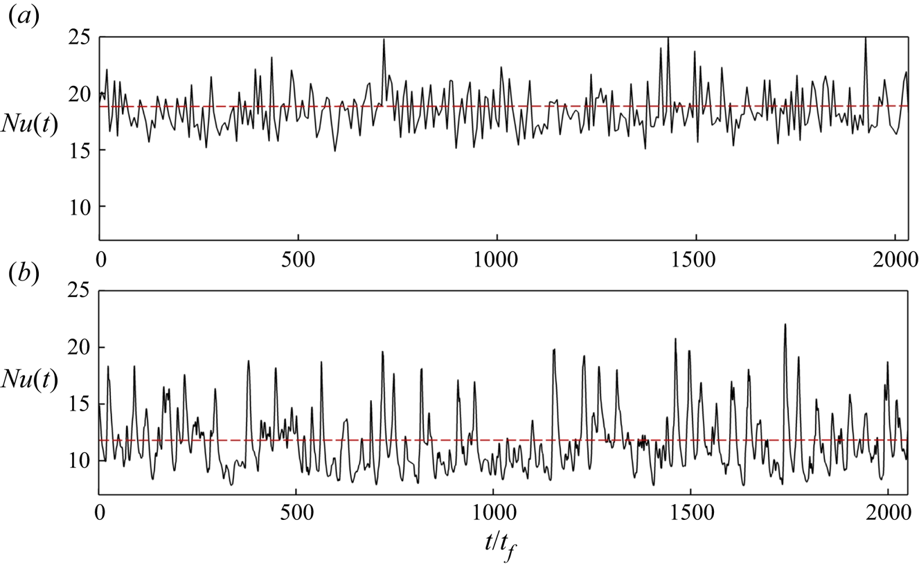
As an example, we plot in figure 4 the time series of the turbulent heat flux for the CHF1 and CHF2 cases, i.e.  $Nu(t)={1}/({\langle T(t) \rangle _{A}|_{z=0}-\langle T(t) \rangle _{A}|_{z=1}})$ over a time interval of the same length. In both cases, the Nusselt numbers are fluctuating strongly, which is typical for slender convection cells. It is seen that the fluctuation level is smaller for
 $Pr=0.7$ than
 $Pr=0.033$ since coarser thermal plumes exist at lower
 $Pr$. In CHF1 to CHF3, the turbulent heat transport is increased slightly in comparison to the three corresponding RBC cases, which is consistent with the DNS at the lower Rayleigh numbers in Verzicco & Sreenivasan (Reference Verzicco and Sreenivasan2008) and in Johnston & Doering (Reference Johnston and Doering2009).
Time evolution of the Nusselt number  $Ra=10^7$, and
 $\varGamma =1/2$ for the case of constantly prescribed heat flux (CHF) at the boundaries. The Nusselt number is defined by (3.3) for
 $(a)$
 $Pr=0.7$ and
 $(b)$
 $Pr=0.033$. The dashed line represents the mean value. In these two cases, the simulations have been run longer as listed in table 2 with a very sparse output. The mean values agree with those in the table.

We finally discuss  $Nu$ for the case of conjugate heat transfer setting using (3.2). The turbulent heat transfer is found to be largest in CHT cases and smallest in RBC cases for a given parameter pair
 $(Ra, Pr)$. Nusselt numbers are enhanced by 19 % for convection in air (
 $Pr=0.7$), by 12 % for convection in GaInSn (
 $Pr=0.033$) at
 $Ra=10^7$, and by 13 % at
 $Ra=10^8$. The results of numerical simulation by Smirnov, Smirnov & Smirnovsky (Reference Smirnov, Smirnov and Smirnovsky2017) show an enhancement of 8 %–10 % for
 $Nu$ in cylindrical cell with
 $\varGamma =1$ for mercury (
 $Pr=0.025$) when the top and bottom cell bounded by steel plates. Teimurazov & Frick (Reference Teimurazov and Frick2017) also found an increase of
 $Nu$ by 12 % in their cylindrical cell with
 $\varGamma =0.2$ using liquid sodium (
 $Pr=0.008$) for
 $Ra= 5\times 10^6$, when BCs were changed from RBC to CHF. Results obtained in an experimental apparatus of same geometry by Vasil'ev et al. (Reference Vasil'ev, Kolesnichenko, Mamykin, Frick, Khalilov, Rogozhkin and Pakholkov2015) yielded an increase of the convective heat flux from
 $Nu=19.6$ to
 $28.6$. Our findings are thus also consistent with previous liquid metal flow investigations, both experimental and numerical ones.
Turbulent transport of momentum is quantified by the Reynolds number, which is defined as
 \begin{equation} Re=\sqrt{\frac{Ra}{Pr}}\, u_{rms,V} \quad \mbox{with} \ u_{rms,V} =\sqrt{\langle u_i^2\rangle_{V,t}}. \end{equation}
The Reynolds numbers are also listed in table 2. With decreasing Prandtl number the Reynolds number is expected to increase at a fixed Rayleigh number, displaying enhanced fluid inertia effects which are caused by an extended energy cascade range as discussed in Schumacher, Götzfried & Scheel (Reference Schumacher, Götzfried and Scheel2015). At  $Ra=10^7$, the Reynolds number
 $Re$ grows here by almost a factor of 10 when switching fluid from air to GaInSn. The Reynolds number values for the three sets of boundary conditions scatter at a parameter pair
 $(Ra, Pr)$ by 9 % for
 $Pr=0.7$, by 2 % for
 $Pr=0.033$ and
 $Ra=10^7$ and by 6 % for
 $Pr=0.033$ and
 $Ra=10^8$. The variability of the global momentum transfer with respect to the thermal BC is thus significantly smaller as that of the global heat transfer. These results are consistent with previous experiments by Huang et al. (Reference Huang, Wang, Xi and Xia2015) who found an increase of
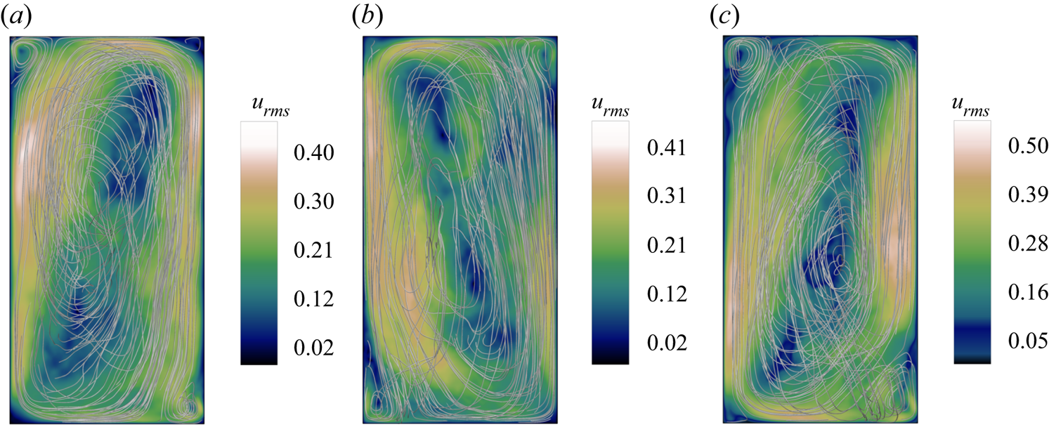
 $Re$ by 9 % when a fixed temperature BC was applied at the bottom of their rectangular cell instead of fixed heat flux. This finding can be interpreted with the help of figure 5 which shows vertical cuts through the cell for
 $Pr=0.033$ and different boundary conditions. In detail, we plot contours of
 $u_{rms}$ for
 $(a)$ RBC2
 $(b)$ CHF2 and
 $(c)$ CHT2, respectively.
The vertical mid plane colour contour maps of root-mean-square velocity  $u_{rms}$ field measured at
 $Ra=10^7$,
 $Pr=0.033$, and
 $\varGamma =1/2$ with different boundary conditions:
 $(a)$ RBC1,
 $(b)$ CHF1 and
 $(c)$ CHT1. The three-dimensional velocity streamlines are superimposed to clarify the LSC orientation with two small counter-rotating rolls at the corners.

Streamlines of the velocity field are added to each of the three panels in figure 5. For all runs, we detected that the large-scale flow varies between two distinct configurations, these are the one-roll and the two-roll structures with a slight preference for the single-roll state (not shown). This property is robust with respect to the different boundary conditions.
4. Comparison of temperature and velocity statistics
4.1. Temperature field
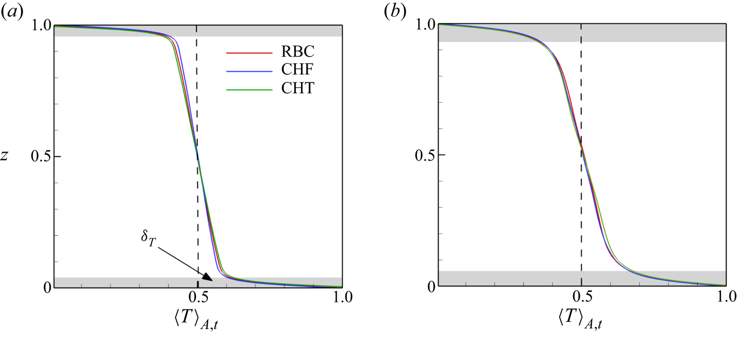
It is well known that the mean temperature profile in thermal convection changes basically across a thin thermal boundary layer with a non-dimensional thickness  $\delta _T = 1/(2Nu)$, while it remains nearly constant in the bulk region. In figure 6, we display the mean temperature profiles
 $\langle T(z)\rangle _{A,t}$ for
 $Pr= 0.7$ (see figure 6a) and
 $Pr=0.033$ (see figure 6b), both at
 $Ra=10^7$. Here,
 $\langle \cdot \rangle _{A,t}$ stands for averaging in horizontal planes
 $A$ and time
 $t$. It is worth mentioning that the mean temperature profiles for the case of CHF are normalized (
 $T_{CHF} = T_{RBC} Nu$). The approximate thermal boundary layer thickness of the three runs is highlighted in grey in both panels and denoted by
 $\delta _T$ in figure 6. The plotted temperature profiles are very similar with a small deviations close to the edge of thermal boundary layers, which is somewhat better visible for
 $Pr=0.7$. All cases show a finite negative slope in the bulk region which indicates that the temperature field is not perfectly mixed by the turbulence in the slender cell.
Averaged profiles of normalized temperature  $\langle T(z)\rangle _{A,t}/\varTheta$ along the vertical axis
 $z$ for
 $Ra=10^7$ and different Prandtl numbers:
 $(a)$
 $Pr=0.7$,
 $(b)$
 $Pr=0.033$. Different thermal boundary conditions are indicated in the legend.

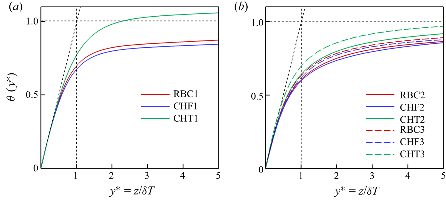
In order to compare the profiles in the vicinity of the bottom plate for different cases better, we plot rescaled mean temperature  $\theta (y^*)$ profiles in figure 7 for all 9 simulation runs. Following Shishkina & Thess (Reference Shishkina and Thess2009) and Scheel & Schumacher (Reference Scheel and Schumacher2016), we apply
 \begin{equation} \theta(y^*) = 2 - 2 \langle T(y^*) \rangle _{A,t} \quad \mathrm{with}\ y^* = z/ \delta_{T}. \end{equation}
The dotted line indicates the slope of one of the profiles close to the wall. We see the profiles are  $Pr$-dependent. The profiles which show a deviation further away from the wall are those for the CHT cases (in comparison to the other cases). Recall that the mean plate temperature can fluctuate. Numerical (e.g. by Verzicco & Sreenivasan Reference Verzicco and Sreenivasan2008) and experimental studies (e.g. by Huang et al. Reference Huang, Wang, Xi and Xia2015) found that the plume emissions are stronger for constant temperature than for constant-heat-flux boundary conditions.


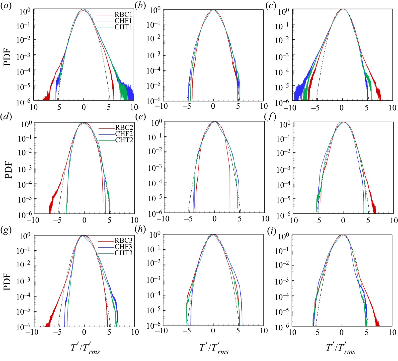
The statistics of the corresponding temperature fluctuations,  $T^{\prime }=T-\langle T(z)\rangle _{A,t}$, are compared in figure 8 by means of the probability density functions (PDFs) taken at different subvolumes in the convection cell. We defined the subvolumes with
 $x,y \in [-0.25,0.25]$ at the bottom
 $z\in [0,0.2]$, bulk
 $z\in [0.4,0.6]$ and top
 $z\in [0.8,1]$. All PDFs of the RBC cases have the strongest positive tail at the bottom and the strongest negative tail at the top which are caused by plume detachments that seem to be more pronounced as for the other thermal boundary conditions. These differences are found in the far tails (see red curves). The distributions are always symmetric in the cell centre which is expected. The distributions remain close to the Gaussian and tend to be even sub-Gaussian. Significant differences with a variation of
 $Ra$ or
 $Pr$ cannot be identified. The temperature statistics at low Prandtl numbers is particularly determined by coarse plume structures and geometric constraints in the slender cell. It can be seen that
 $Ra=10^8$ (see figure 8g–i). The PDFs differ less of each other in the centre, the PDF profiles with imposed constant heat flux are closer to those of the conjugate heat transfer set-up.
Probability density functions of the temperature fluctuations with different boundary conditions: (a–c) for  $Ra=10^7, Pr=0.7$, (d–f) for
 $Ra=10^7, Pr=0.033$ and (g–i) for
 $Ra=10^8$ and
 $Pr=0.033$. Data are taken for subvolume with
 $x,y \in [-0.25,0.25]$ at the bottom
 $z\in [0,0.2]$ in panels (a,d,g), bulk
 $z\in [0.4,0.6]$ in panels (b,e,h) and top
 $z\in [0.8,1]$ in panels (c,f,i). The temperature fluctuations are normalized by the corresponding root mean square values. The legends in each row hold for all three panels. The Gaussian distribution is added to each figure as a black dashed-dotted line.

4.2. Velocity field
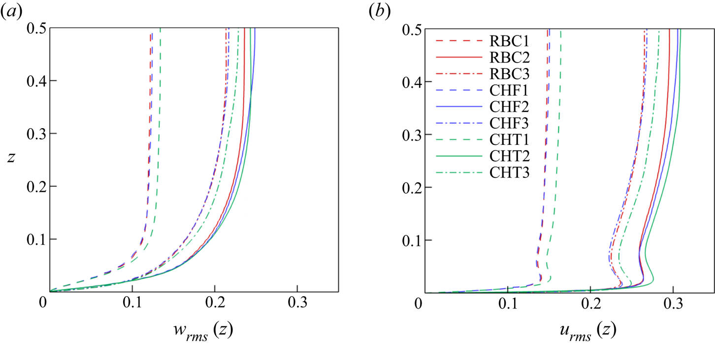
Next, we compare the vertical root-mean-square (r.m.s.) profiles obtained from all three components of the velocity field and their vertical velocity components for different  $Ra, Pr$ and boundary conditions. Note again that
 $u_{rms}(CHF)=\sqrt {Nu}\, u_{rms}(RBC)$. The corresponding r.m.s. values are given by
 \begin{equation} u_{rms}(z)=\sqrt{\langle u_x^2 +u_y^2 +u_z^2 \rangle_{A,t}} \quad\mathrm{and}\quad w_{rms}(z)=\sqrt{\langle u_z^2 \rangle_{A,t}} . \end{equation}
Figure 9 displays our findings. Due to the no-slip BC at the top and bottom plates the fluctuation profiles are zero at the wall. The flow in the bulk region is driven and dominated by a thermal plumes which feed the LSC flow. Thus the velocity field rises in a short distance at the plate from zero to that of the LSC amplitude across the viscous boundary layer thickness. It can be seen that the level of velocity fluctuations for both the three-dimensional  $u_{rms}(z)$ and the vertical
 $w_{rms}(z)$ is significantly enhanced for the lower
 $Pr$ at the same
 $Ra$. The coarser thermal plumes (which are in line with a thicker thermal boundary layer) drive the fluid turbulence starting from a larger scale and extend the inertial cascade range such that the flow Reynolds number is enhanced. The magnitude of both fluctuation profiles decreases at fixed
 $Pr$ for the larger of both
 $Ra$. In figure 9(b), we also observe a local maximum in all profiles at the edge of thermal BLs, where thermal plumes detach from the plates and rise into the bulk of the cell. We found that for the RBC and CHF cases
 $u_{rms}(z)$ is practically similar in the boundary layers. The differences between all three cases remain small and do not exceed a few per cent in magnitude.
Root-mean-square velocity profiles for all 9 simulation runs.  $(a)$ Vertical velocity component root-mean-square profile
 $w_{rms}(z)$.
 $(b)$ Total root-mean-square velocity profile
 $u_{rms}(z)$. The legend holds for both (a,b). See table 2 for the labelling. Since the statistical fluctuations are symmetric with respect to the midplane at
 $z=0.5$, we plot the arithmetic average of the profiles of the lower and upper halves.

5. Boundary layer analysis
As already said in the introduction, low- $Pr$ experiments typically apply copper plates at the top and bottom (e.g. Cioni et al. Reference Cioni, Ciliberto and Sommeria1997; Horanyi et al. Reference Horanyi, Krebs and Müller1999; Huang et al. Reference Huang, Wang, Xi and Xia2015; Vasil'ev et al. Reference Vasil'ev, Kolesnichenko, Mamykin, Frick, Khalilov, Rogozhkin and Pakholkov2015; Zürner et al. Reference Zürner, Schindler, Vogt, Eckert and Schumacher2019), which have thermal conductivities that are only an order of magnitude larger than those of the liquid metal (see table 1). The rapid re-establishment of a uniform plate temperature after local plume detachments should ideally proceed by heat conduction inside the plate, and not via the working fluid. In this section, we therefore want to investigate how spatial temperature variations very close to the walls, which are probed by temperature gradients, differ for the three different sets of BCs. Without discussing further details, we point here to an alternative experimental set-up that establishes a better temperature equilibration in the plates by Zwirner et al. (Reference Zwirner, Khalilov, Kolesnichenko, Mamykin, Mandrykin, Pavlinov, Shestakov, Teimurazov, Frick and Shishkina2020).
5.1. Local thermal boundary layer thickness
The strongest local temperature gradient magnitudes will generally be also confined to the boundary layers near the bottom and top plates. The mean thickness of boundary layer can be defined in several ways. The standard way with  $\delta _T=1/(2 Nu)$ was discussed in § 3. The alternative way is via a refined local analysis. Such detailed numerical studies of local thermal boundary layer thicknesses in turbulent RBC in cylindrical cells with aspect ratio one were reported in Scheel & Schumacher (Reference Scheel and Schumacher2014), where the inverse of the magnitude of the vertical temperature derivative at the plate, a local slope, was associated with a local thermal boundary layer thickness, given in dimensionless form by
 \begin{equation} \lambda_T(x,y)=\left.\frac{1}{2}\right| \left.\frac{\partial T}{\partial z} \right|_{z=0,1}^{-1}. \end{equation}
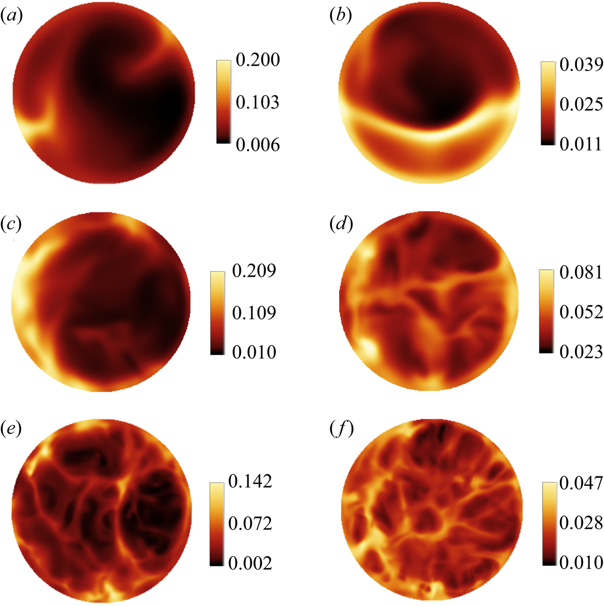
Equation (5.1) gives the inverse local slope of the temperature at each point of the plate. To shed more light on the effect of thermal BCs on the local boundary layer scales, we display contours of instantaneous plots of  $\lambda _T(x,y,0)$ for RBC and CHT cases in figure 10. The left column is for RBC and the right column for CHT. Figure 10(a–d) plots data for
 $Ra=10^7$ and figure 10(e,f) for
 $Ra=10^8$. The first row shows the case of
 $Pr=0.7$ while the second and third rows display the analysis for
 $Pr=0.033$. In all cases, we observe a spatial variation across the plate with largest values close to the sidewalls where the thermal plumes detach and rise preferentially with the LSC. As the Rayleigh number is increased to
 $10^8$, the structures become more filamented. It is interesting to see that the range of values of the local thicknesses is about the same for both RBC cases in figures 10(a) and 10(c) at first glance and that the area fraction of high amplitude events is larger for the lower Prandtl number which results in a larger mean value. Also observed is a slightly larger spatial variability in cases of the lower Prandtl number which is in line with the more complex wall stress field structure as analysed for example by Schumacher et al. (Reference Schumacher, Bandaru, Pandey and Scheel2016). For the CHT cases, the heat injection depends on the ratio of the conductivities of the fluid and the plate. Thus this case should be more prone to Prandtl-number variations as visible in figures 10(b) and 10(d) at the same
 $Ra$ number.
Snapshots of the local thermal boundary layer scale  $\lambda _T(x,y)$, as given by (5.1) at the bottom plate. Fixed-temperature boundary condition is applied in: (a,b) RBC1 and CHT1 at
 $Pr=0.7$; (c,d) RBC 2 and CHT2 at
 $Pr=0.033$; (e,f) RBC3 and CHT3 at
 $Pr=0.033$ and
 $Ra=10^8$. The colour bars indicate the magnitude of
 $\lambda _T$ in each case. All local boundary layer thicknesses are measured in units of
 $H$.

The mean value of the local thicknesses  $\lambda _T(x,y)$ follows as an ensemble average and is given by
 \begin{equation} \langle \lambda_T \rangle=\int_{0}^{\infty}\lambda_T\,p(\lambda_T)\,\textrm{d}\lambda_T=\frac{1}{2}\left\langle \left| \frac{\partial T}{\partial z} \right|_{z=0,1}^{-1}\right\rangle, \end{equation}
where  $p(\lambda _T)$ is the PDF of the local scales
 $\lambda _T(x,y)$. When comparing this mean thickness with the standard
 $\delta _T=1/(2 Nu)$, we obtain the following: for RBC1
 $(\langle \lambda _T\rangle ,\delta _T)=(0.043,0.029)$, for case RBC2
 $(0.067,0.047)$, and for RBC3
 $(0.036,0.023)$. Furthermore, for case CHT1 we get
 $(0.027,0.023)$, for CHT2
 $(0.043,0.041)$ and finally for CHT3
 $(0.021,0.020)$. It is seen that the values of
 $\langle \lambda _T\rangle$ are somewhat overestimated in the RBC case as already found in Scheel & Schumacher (Reference Scheel and Schumacher2014). The values agree consistently for the three CHT cases as we match the fluxes at the plate–fluid interfaces.
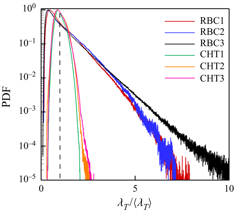
In figure 11, we plot the results of the rescaled PDFs of the local BL scales for the RBC and CHT cases as given in (5.1) and (5.2). The distribution for the CHF case would be a delta function,  $p(\lambda _T/\langle \lambda _T\rangle )=\delta (\lambda _T/\langle \lambda _T\rangle -1)$. The data are taken over the whole cross-section of the plate and for long sequences of snapshots. We see in both cases that the dependence on the Prandtl number remains small when data are compared for each set of boundary conditions. The PDFs remain practically similar even though the tails are slightly extended only for the lower
 $Pr$. A main difference is the shift of the maximum of the PDF from
 $\lambda _T/\langle \lambda _T\rangle <1$ in RBC to
 $\lambda _T/\langle \lambda _T\rangle \approx 1$ in CHT. This is in line with a fatter tail in the RBC case that indicates a much stronger variability of the local scales. An additional increase of the Rayleigh number from
 $10^7$ to
 $10^8$ in the RBC set-up leads to a significantly fatter tail indicating enhanced fluctuations of the local BL thickness. The shape and the trend with Rayleigh number are found to agree with Scheel & Schumacher (Reference Scheel and Schumacher2014). This is the first significant difference when finitely thick plates are applied instead of the idealized thin ones.
Probability density functions of the local thermal boundary layer scale  $\lambda _T(x,y)$ given in units the corresponding mean thickness
 $\langle \lambda _T\rangle$. Data are combined for the three RBC and CHT cases. The notation corresponds to table 2. The PDFs are obtained over a sequence of snapshots and the whole bottom and top plates. The vertical dashed line is for
 $\lambda _T/\langle \lambda _T\rangle =1$.

5.2. Local viscous boundary layer thickness
Similarly one can proceed for the viscous boundary layer thickness of the velocity field. The local velocity boundary scale  $\lambda _v(x,y)$ and its mean value
 $\langle \lambda _v(x,y)\rangle$ are defined as
 \begin{equation} \lambda_v(x,y)= u_{rms} \left| \frac{\partial \boldsymbol{u}^{(2)}}{\partial z} \right|_{z=0,1}^{-1} \quad\mathrm{and}\quad \langle \lambda_v \rangle = u_{rms}\left\langle \left| \frac{\partial \boldsymbol{u}^{(2)}}{\partial z} \right|_{z=0,1}^{-1}\right\rangle, \end{equation}
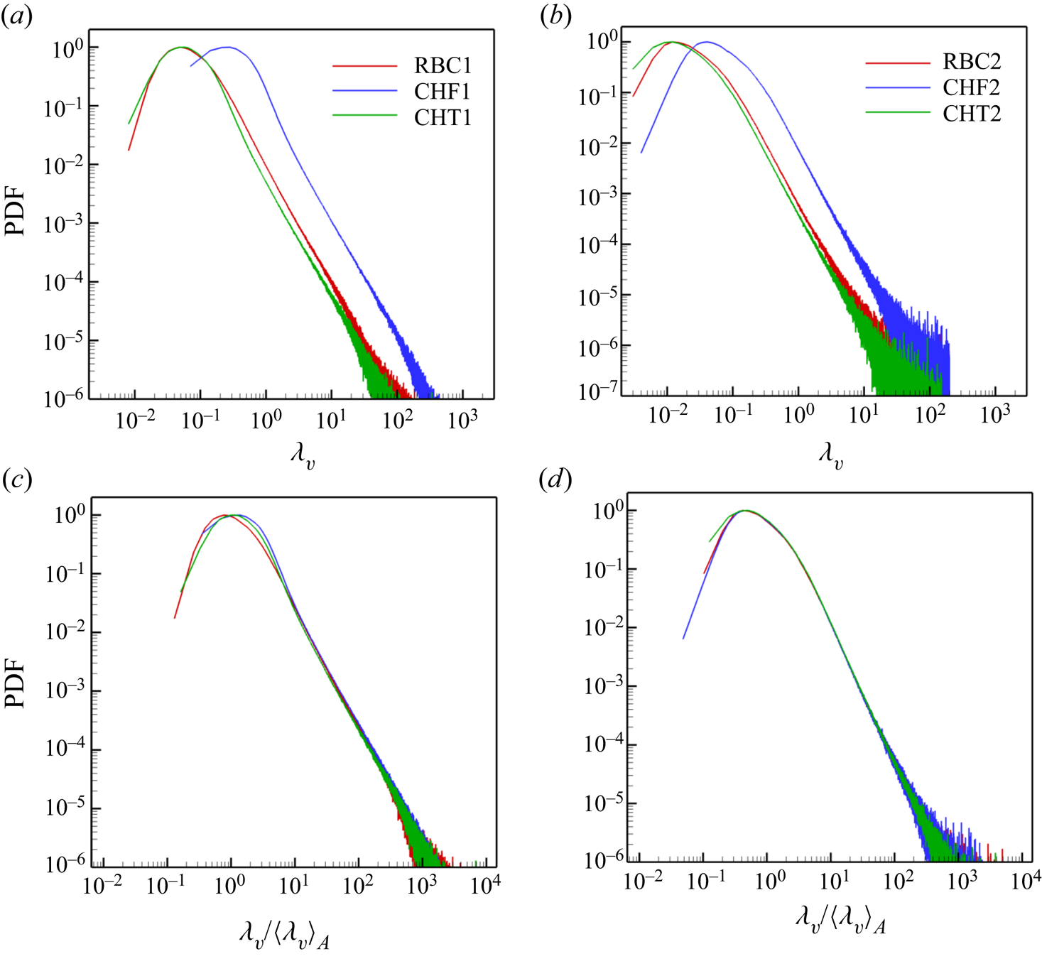
where  $\boldsymbol {u}^{(2)}=(u_x,u_y)$ and zero derivatives are excluded. In figure 12(a,b) we plot the results of the PDFs of
 $\lambda _v$ and in figure 12(c,d) we replot the data rescaled with their respective means
 $\langle \lambda _v\rangle$ as given in (5.3a,b). Figure 12(a,c) for
 $Pr=0.7$, figure 12(b,d) for
 $Pr=0.033$. Comparing the results in figure 12(a,b), we find that the velocity boundary layer thicknesses are on average smaller for the liquid metal case than for air which is in line with the larger Reynolds number reported for these cases in table 2. Interestingly, for given
 $Ra$ and
 $Pr$ numbers, we find that the local velocity boundary layer distributions with respect to
 $\lambda _v$ for RBC and CHT collapse, and that they are shifted in comparison to the CHF cases. As can also be seen, all re-scaled PDFs in figure 12(c,d) collapse well and are in good agreement with the findings in Scheel & Schumacher (Reference Scheel and Schumacher2014).
Probability density functions (PDFs) of the local outer velocity boundary layer thickness  $\lambda _v$ of all simulation data for
 $Ra=10^7, \varGamma =1/2$: (a,c) for
 $Pr=0.7$ and (b,d) for
 $Pr=0.033$. In the (c,d) cases, we scaled each PDF by its mean value as given in (5.3a,b). Data are obtained over a sequence of snapshots and the whole bottom and top plates. See table 2 for the legend name. The behaviour of the data at
 $Ra=10^8$ is similar and thus not displayed. All distributions collapse again when rescaled by the mean thickness.

6. Summary and outlook
In the present work, we have studied the effect of different temperature boundary conditions on thermal convection in a cylinder with  $\varGamma =1/2$ using air and liquid metal as working fluid at Rayleigh numbers
 $Ra=10^7$ and
 $10^8$. Three different thermal boundary conditions have been applied at the top and bottom plates, (i) constant temperature (RBC), (ii) constant heat flux (CHF) and (iii) conjugated heat transfer (CHT). All three cases have thermally insulated sidewalls and no-slip boundary conditions for the velocity field. The magnitude of heat and momentum transfer follows the same trend in all three cases with a decrease of the Prandtl number. While turbulent heat transfer is decreased, turbulent momentum transfer is significantly increased. The transport behaviour of the three cases at fixed Rayleigh and Prandtl numbers can be summarized as follows: the turbulent heat transfer is enhanced for the constant flux and conjugate heat transfer cases in comparison to the standard fixed-temperature case. This finding is consistent with results by Smirnov et al. (Reference Smirnov, Smirnov and Smirnovsky2017), who found an enhancement of
 $Nu$ by 10 % when their cylindrical cell is bounded by steel plates. It is also in agreement (although not directly comparable) with the lower Rayleigh number cases of Verzicco & Sreenivasan (Reference Verzicco and Sreenivasan2008) and Johnston & Doering (Reference Johnston and Doering2009). The global momentum transfer is less sensitive to a change of boundary conditions of the temperature field as can be seen by the smaller variation of the Reynolds number in table 2. This holds for (i) a switch from the higher to the lower Prandtl number at fixed Rayleigh number as well as for (ii) a switch to a higher Rayleigh number at constant Prandtl number. This is understandable since the majority of the thermal plumes which drive the fluid turbulence at a given
 $(Ra, Pr)$ provide a similar broadband forcing. We have also detected the essentially same behaviour of the large-scale flow in all cases, including the well-known switches between single-roll and double-roll configurations.
From the global statistical perspective considered, we find surprisingly small differences in the mean temperature profiles in particular for the low-Prandtl-number cases. The same holds for the statistical distribution of the fluctuations of the temperature field and the profiles root mean square velocity  $u_{rms}$ as well as its vertical component
 $w_{rms}$. These profiles remain closely together for each
 $(Ra, Pr)$. The PDFs display asymmetric far tails when the temperature field is less diffusive, i.e. when the Prandtl number is larger. Furthermore, we confirm that for all three sets of thermal boundary conditions, the lower of the two Prandtl numbers leads to larger amplitudes of the velocity fluctuations, i.e. this characteristic property of a low-Prandtl-number convection flow remains robust.
As expected, the strongest differences are found when the local structure of the thermal boundary layer is monitored. Here, we apply the concept of the local thermal boundary layer thickness, which is defined via the vertical temperature derivative at the plates. The probability density functions of these local scales differ significantly when the RBC and CHT cases are compared. The RBC case is found to have a fat tail towards larger scales. The distribution is much narrower when heat fluxes are matched at the top and bottom (and it is by definition a delta function when the flux is constant and prescribed). The effect of the Prandtl number remains small, as shown by the collapse of the distributions of the rescaled thicknesses. A similar procedure for a local viscous boundary layer thickness displays also a nearly perfect collapse.
To conclude our analysis, the differences in the three cases turn out to remain relatively small when global quantities of turbulent convection are probed. This is particularly true from an experimental perspective, where the access to the inner structure of the boundary layers remains challenging and is for high Rayleigh numbers and low Prandtl numbers practically impossible. We cannot exclude that the differences will grow as the Rayleigh numbers in liquid metal convection are increased. These efforts are part of our future research.
Acknowledgements
We thank J.D. Scheel for several useful discussions. N.F. and D.K. are supported by the Deutsche Forschungsgemeinschaft with grants no. SCHU 1410/29-1 and KR 4445/2-1, respectively. We acknowledge support with computing resources by the Large Scale Project No. pn68ni of the Gauss Centre for Supercomputing. The simulations were carried out on the SuperMUC-NG compute cluster at the Leibniz Rechenzentrum Garching (Germany).
Declaration of interests
The authors report no conflict of interest.