



1 Introduction
1.1 Nonlinear dynamics of viscoelastic liquid jets
Non-Newtonian viscoelastic liquid jets are often encountered in applications such as inkjet printing, fuel atomization, micro/nano-fibre manufacture, industrial prilling, microfluidics, pharmaceuticals and rheological measurements (Eggers & Villermaux Reference Eggers and Villermaux2008; Zell et al. Reference Zell, Gier, Rafaï and Wagner2010; Basaran, Gao & Bhat Reference Basaran, Gao and Bhat2013; Alsharif, Uddin & Afzaal Reference Alsharif, Uddin and Afzaal2015). The study of the instability and break-up of viscoelastic jets is of both theoretical and practical interest. Upon a small axisymmetric disturbance being imposed, a jet is perturbed and starts to deform. It has been well recognized that the growth of the disturbance at initial times can be predicted by linear theory (Rayleigh Reference Rayleigh1878, Reference Rayleigh1879). However, as the deformation of the jet grows, a nonlinear effect comes into play. Particularly for a viscoelastic jet, due to viscoelasticity, break-up can be greatly postponed: the jet experiences a slow necking process and evolves into a quasistatic beads-on-a-string structure with large primary droplets connected by a thin filament, sometimes accompanied by small secondary droplets between the primary ones (Bousfield et al. Reference Bousfield, Keunings, Marrucci and Denn1986; Entov & Hinch Reference Entov and Hinch1997; Chang, Demekhin & Kalaidin Reference Chang, Demekhin and Kalaidin1999; Anna & McKinley Reference Anna and McKinley2001; Christanti & Walker Reference Christanti and Walker2001, Reference Christanti and Walker2002; Clasen et al. Reference Clasen, Eggers, Fontelos, Li and McKinley2006; Oliveira, Yeh & McKinley Reference Oliveira, Yeh and McKinley2006; Malkin, Arinstein & Kulichikhin Reference Malkin, Arinstein and Kulichikhin2014; Wagner, Bourouiba & McKinley Reference Wagner, Bourouiba and McKinley2015; Deblais, Velikov & Bonn Reference Deblais, Velikov and Bonn2018).
To date the nonlinear behaviour of viscoelastic jets has been extensively studied theoretically, numerically and experimentally. To facilitate the theoretical and numerical aspects, many researchers employed one-dimensional (1-D) viscoelastic models based on the slender body approximation (Bousfield et al.
Reference Bousfield, Keunings, Marrucci and Denn1986; Schümmer & Thelen Reference Schümmer and Thelen1988; Chang et al.
Reference Chang, Demekhin and Kalaidin1999; Li & Fontelos Reference Li and Fontelos2003; Clasen et al.
Reference Clasen, Eggers, Fontelos, Li and McKinley2006; Ardekani, Sharma & McKinley Reference Ardekani, Sharma and McKinley2010; Bhat et al.
Reference Bhat, Appathurai, Harris, Pasquali, McKinley and Basaran2010, Reference Bhat, Appathurai, Harris and Basaran2012). The validity of these 1-D viscous or viscoelastic models has been examined and justified by comparing with the two-dimensional (2-D) algorithms and experimental results (Ambravaneswaran, Wilkes & Basaran Reference Ambravaneswaran, Wilkes and Basaran2002; López-Herrera & Gañán-Calvo Reference López-Herrera and Gañán-Calvo2004; Wagner et al.
Reference Wagner, Amarouchene, Bonn and Eggers2005; Collins, Harris & Basaran Reference Collins, Harris and Basaran2007; Eggers & Villermaux Reference Eggers and Villermaux2008; Tembely et al.
Reference Tembely, Vadillo, Mackley and Soucemarianadin2012; Turkoz et al.
Reference Turkoz, Lopez-Herrera, Eggers, Arnold and Deike2018). In the 1-D analyses, the most significant finding is the scaling laws followed by the thinning of the filament for a viscoelastic jet of Oldroyd-B type. That is, the thickness of the filament decreases exponentially with time at a rate of
 $1/3De$
(
 $De$
is the Deborah number defined as the ratio of the stress relaxation time to the capillary time), whereas the polymeric stress inside the filament increases exponentially with time at the same rate (Chang et al.
Reference Chang, Demekhin and Kalaidin1999; Clasen et al.
Reference Clasen, Eggers, Fontelos, Li and McKinley2006). Besides, the self-similarity in the corner region joining the droplet to the filament was explored theoretically with the aid of 1-D models (Clasen et al.
Reference Clasen, Eggers, Fontelos, Li and McKinley2006; Bhat et al.
Reference Bhat, Appathurai, Harris and Basaran2012). The dynamics of droplets in highly stretched viscoelastic jets was investigated by Li & Fontelos (Reference Li and Fontelos2003). The formation of satellite droplets in beads-on-a-string structures as well as the way to eliminate them was explored by Ardekani et al. (Reference Ardekani, Sharma and McKinley2010) and Bhat et al. (Reference Bhat, Appathurai, Harris, Pasquali, McKinley and Basaran2010). Beyond Oldroyd-B liquids, other types such as upper-convected Jeffreys, Giesekus and FENE-P fluids were also examined (Schümmer & Thelen Reference Schümmer and Thelen1988; Fontelos & Li Reference Fontelos and Li2004; Ardekani et al.
Reference Ardekani, Sharma and McKinley2010).
In addition to the 1-D studies, a few direct numerical simulations have been carried out. Morrison & Harlen (Reference Morrison and Harlen2010) used a Lagrangian–Eulerian finite-element method to simulate the deformation and break-up of FENE-CR viscoelastic liquid flows ejected from a nozzle in the drop-on-demand inkjet printing process. Gupta & Chokshi (Reference Gupta and Chokshi2015) conducted a weakly nonlinear stability analysis of the extensional flow of an extended Pom-Pom polymer jet perturbed by a finite-amplitude disturbance. Using the volume-of-fluid method to track the interface and the log-conformation transformation to solve the constitutive equation, Turkoz et al. (Reference Turkoz, Lopez-Herrera, Eggers, Arnold and Deike2018) performed a direct numerical simulation of the axisymmetric thinning of a viscoelastic filament of Oldroyd-B liquid. Their 2-D simulations provided some details of the velocity and the stresses in the entire thread.
The relevant experimental investigation is much more prosperous. A great number of experiments have been dedicated to the capillary thinning and break-up of viscoelastic liquid jets (Tirtaatmadja, McKinley & Cooper-White Reference Tirtaatmadja, McKinley and Cooper-White2006; Bazilevskii & Rozhkov Reference Bazilevskii and Rozhkov2014; Kulichikhin et al. Reference Kulichikhin, Malkin, Semakov, Skvortsov and Arinstein2014; Malkin et al. Reference Malkin, Arinstein and Kulichikhin2014; Greiciunas et al. Reference Greiciunas, Wong, Gorbatenko, Hall, Wilson, Kapur, Harlen, Vadillo and Threlfall-Holmes2017; Jimenez et al. Reference Jimenez, Dinic, Parsi and Sharma2018; Mathues et al. Reference Mathues, Formenti, McIlroy, Harlen and Clasen2018; Varchanis et al. Reference Varchanis, Dimakopoulos, Wagner and Tsamopoulos2018). These experimental studies elucidated the nonlinear pinch-off dynamics of viscoelastic jets, the formation of primary and satellite droplets, the extensional rheological properties of viscoelastic liquids, the effect of the molecular weight and concentration of the polymer, the phase separation phenomenon, as well as the feasibility and productivity of extensional flows in distinct applications such as inkjet printing, fibre spinning, rheometers and blood plasma. Among them, Wagner et al. (Reference Wagner, Amarouchene, Bonn and Eggers2005) found that the addition of a small amount of polymer may significantly delay the detachment of a water drop and lead to the formation of a long-lived filament with secondary beads on it in certain conditions. Clasen et al. (Reference Clasen, Bico, Entov and McKinley2009) explored the mechanism in the transition from dripping to jetting and found that the viscoelastic filament exerts an axial tensile force on the adjacent drops, which, together with the capillary, inertial and gravitational forces, controls the detachment of the terminal drop. Sattler, Wagner & Eggers (Reference Sattler, Wagner and Eggers2008), Sattler et al. (Reference Sattler, Gier, Eggers and Wagner2012), Kulichikhin et al. (Reference Kulichikhin, Malkin, Semakov, Skvortsov and Arinstein2014), and Eggers (Reference Eggers2014) studied the blistering pattern with different generations of small droplets on the filament as well as the instability and phase separation in it.
1.2 Nonlinear dynamics of electrified liquid jets
In electrospraying and electrospinning experiments, the electric field has been shown to be a novel, easy way to control the linear and nonlinear behaviour of liquid jets (Yu, Fridrikh & Rutledge Reference Yu, Fridrikh and Rutledge2006; Eda & Shivkumar Reference Eda and Shivkumar2007; Ismail et al. Reference Ismail, Maksoud, Ghaddar, Ghali and Tehrani-Bagha2016; Wang, Wang & Hashimoto Reference Wang, Wang and Hashimoto2016; Wang et al. Reference Wang, Hashimoto, Li, Li and Wang2018). The coupling of the electric field with the flow field gives rise to new phenomena of instability and rupture of jets, and exploring the underlying mechanisms undoubtedly enriches the fundamentals in electrokinetics and electrohydrodynamics. On the other hand, owing to simplicity, efficiency and flexibility in producing monodisperse droplets and ultra-thin fibres at micro/nanometre scales, electrified jets are very popular in various applications involving electrohydrodynamic, electrochemical or biomechanical processes. The relevant experimental studies are too numerous to mention. To gain a comprehensive understanding of those fundamentals in physics and the latest progress in diverse applications, the interested readers are referred to several recent reviews contributed by Onses et al. (Reference Onses, Sutanto, Ferreira and Alleyne2015), Gañán-Calvo et al. (Reference Gañán-Calvo, López-Herrere, Herrada, Ramos and Montanero2018), Rosell-Llompart, Grifoll & Loscertales (Reference Rosell-Llompart, Grifoll and Loscertales2018) and Yoon et al. (Reference Yoon, Yang, adn and Yu2018).
Due to the complexity of the problem, only a few theoretical and numerical reports have addressed the nonlinear axisymmetric instability of electrified jets in the literature. As in the study of viscoelastic jets, 1-D models were used to facilitate theoretical analysis and save computational time (López-Herrera, Gañán-Calvo & Perez-Saborid Reference López-Herrera, Gañán-Calvo and Perez-Saborid1999; Feng Reference Feng2003; Elcoot Reference Elcoot2007; Wang, Mählmann & Papageorgiou Reference Wang, Mählmann and Papageorgiou2009; Li, Yin & Yin Reference Li, Yin and Yin2016, Reference Li, Yin and Yin2017b ). Among them, López-Herrera et al. (Reference López-Herrera, Gañán-Calvo and Perez-Saborid1999) developed a 1-D model to investigate the nonlinear deformation and break-up of an electrically charged viscous liquid jet of infinite conductivity. Feng (Reference Feng2003) studied the stretching of a straight electrically charged viscoelastic jet of Giesekus liquid. Wang et al. (Reference Wang, Mählmann and Papageorgiou2009) simulated the axisymmetric nonlinear dynamics of a perfectly conducting, viscous liquid jet under the action of a radial electric field. Li et al. (Reference Li, Yin and Yin2016) built a 1-D model to study the nonlinear behaviour of a perfectly conducting, slightly viscoelastic liquid jet under a radial electric field. Later, they investigated the transition from beads-on-a-string to spike structure under a sufficiently large electric field (Li et al. Reference Li, Yin and Yin2017b ). As in a viscous flow (Wang et al. Reference Wang, Mählmann and Papageorgiou2009), the singular spike structure arising in a viscoelastic jet was found to possess a self-similar characteristic.
Some direct numerical simulations have been performed (Setiawan & Heister Reference Setiawan and Heister1997; Higuera Reference Higuera2003, Reference Higuera2006; Collins et al. Reference Collins, Harris and Basaran2007; Wang & Papageorgiou Reference Wang and Papageorgiou2011; Wang Reference Wang2012; López-Herrera et al. Reference López-Herrera, Gañán-Calvo, Popinet and Herrada2015; Lakdawala, Sharma & Thaokar Reference Lakdawala, Sharma and Thaokar2016). Setiawan & Heister (Reference Setiawan and Heister1997) utilized the boundary element method to calculate the time-dependent evolution of a perfectly conducting, inviscid liquid jet subjected to a radial electric field. Higuera (Reference Higuera2003, Reference Higuera2006) numerically simulated the cone-to-jet structure of a conducting viscous liquid jet in electrospraying. Collins et al. (Reference Collins, Harris and Basaran2007) developed a robust Galerkin finite-element algorithm to solve the 2-D Navier–Stokes equation and Laplace equation governing the axisymmetric deformation and break-up of a perfectly conducting, incompressible Newtonian liquid jet under a radial electric field. With the aid of the boundary integral method, Wang & Papageorgiou (Reference Wang and Papageorgiou2011) studied the axisymmetric break-up of a perfectly conducting, viscous liquid thread immersed in another non-conducting, viscous liquid, in the limit of zero Reynolds number. Later, Wang (Reference Wang2012) extended this study to the poorly conducting case. Using a volume-of-fluid method, López-Herrera et al. (Reference López-Herrera, Gañán-Calvo, Popinet and Herrada2015) simulated the break-up of an electrically charged liquid jet at time scales comparable to or smaller than the diffusion and electroosmotic migration times. Lakdawala et al. (Reference Lakdawala, Sharma and Thaokar2016) presented a dual grid level set method (DGLSM) to numerically study the nonlinear break-up dynamics of a perfectly conducting, Newtonian viscous liquid jet under a radial electric field.
1.3 The present work
In the present work we incorporate the Oldroyd-B viscoelastic model with the Taylor–Melcher leaky dielectric theory and elaborate on the nonlinear dynamics of an electrically charged viscoelastic liquid jet of finite conductivity. The Oldroyd-B model, which requires constant viscosity and high elasticity of the liquid, is the simplest nonlinear viscoelastic model suitable to describe large deformations of dilute polymer solutions (Prilutski et al. Reference Prilutski, Gupta, Sridhar and Ryan1983; James Reference James2009). It has been successfully used to investigate the asymptotic behaviour, scaling laws and self-similar characteristic at the late stages of capillary thinning of viscoelastic liquid jets (Chang et al. Reference Chang, Demekhin and Kalaidin1999; Clasen et al. Reference Clasen, Eggers, Fontelos, Li and McKinley2006; Ardekani et al. Reference Ardekani, Sharma and McKinley2010; Bhat et al. Reference Bhat, Appathurai, Harris, Pasquali, McKinley and Basaran2010; Turkoz et al. Reference Turkoz, Lopez-Herrera, Eggers, Arnold and Deike2018). The disadvantage of the model is that it cannot describe the final pinch-off of a viscoelastic jet, for its hypothesis of infinite extensibility of macromolecular chains. To study the pinch-off of viscoelastic jets, a more complicated constitutive equation that allows finite extensibility should be used, such as the Giesekus or FENE-P model. Nevertheless, for primary research on the deformation process of an electrified viscoelastic jet from the initial to large times, the Oldroyd-B model is appropriate. In electrohydrodynamics, the Taylor–Melcher leaky dielectric theory has been widely used to formulate flows of poorly conducting liquids. It consists of the Navier–Stokes equation describing fluid motion, an expression for the conservation of bulk electric current, an equation describing the conservation of surface charge, the Gauss law and the balance of forces on a fluid–fluid interface (Melcher & Taylor Reference Melcher and Taylor1969; Saville Reference Saville1997; Gañán-Calvo et al. Reference Gañán-Calvo, López-Herrere, Herrada, Ramos and Montanero2018). The theory states that there is no charge in the fluid bulk. All charges are located on the interface between the fluids, and only on the interface does the electric field couple with the flow field. Different from a perfect conductor, for which the electrical force is perpendicular to the interface, a leaky dielectric permits the existence of a tangential electric field and tangential electrical force on the interface, which may influence the fluid motion significantly.
The paper is organized as follows. In § 2, the 1-D model is presented. In § 3, the equations and boundary conditions are solved numerically by means of a hybrid algorithm; different nonlinear structures are identified, the mechanisms in the formation of the structures are elucidated and the domains in the plane of the axial wavenumber and the electrical Bond number are delineated; the effect of finite conductivity on the beads-on-a-string and the spike structures is illustrated; the difference between the finite conductivity and large conductivity cases is discussed. In § 4, an experimental observation of the spike structure is presented. In § 5, the main conclusion is drawn.
Schematic of the theoretical model.

2 One-dimensional model
Consider an infinitely long cylindrical liquid jet of radius
 $R$
and velocity
 $U$
surrounded by quiescent atmospheric air, as sketched in figure 1. For mathematical convenience, a relative cylindrical coordinate system
 $(r,\unicode[STIX]{x1D703},z)$
moving together with the jet is used to formulate the problem, where
 $r$
,
 $\unicode[STIX]{x1D703}$
and
 $z$
are the radial, azimuthal and axial coordinates, respectively. The hydrodynamic effect of the air, as well as the effect of the gravitational force, temperature, mass transfer and magnetic field, is neglected. In practical applications such as inkjet printing, electrospraying and electrospinning, a viscoelastic liquid jet emitted from a capillary tube or the tip of a Taylor cone is inevitably accompanied by unrelaxed elastic stresses. The unrelaxed stresses have been shown to play a significant role in the instability and nonlinear behaviour of viscoelastic jets (Ruo et al.
Reference Ruo, Chen, Chang and Chen2012; Mohamed et al.
Reference Mohamed, Herrada, Gañán-Calvo and Montanero2015; Mathues et al.
Reference Mathues, Formenti, McIlroy, Harlen and Clasen2018). Nevertheless, in the present study, we focus on the effect of finite conductivity on the nonlinear evolution of charged viscoelastic jets, and simply assume that there is no unrelaxed elastic stress in the base flow.
The liquid is assumed to be a dilute polymer solution of Oldroyd-B type. For an Oldroyd-B viscoelastic liquid, the deviatoric stress
 $\unicode[STIX]{x1D749}$
can be decomposed into two parts, i.e.
 $\unicode[STIX]{x1D749}=\unicode[STIX]{x1D749}_{s}+\unicode[STIX]{x1D749}_{p}$
, where
 $\unicode[STIX]{x1D749}_{s}$
and
 $\unicode[STIX]{x1D749}_{p}$
are the contributions from the solvent and the polymer to the stress, respectively (James Reference James2009). The constitutive equation for the solvent stress
 $\unicode[STIX]{x1D749}_{s}$
is
 $$\begin{eqnarray}\displaystyle \unicode[STIX]{x1D749}_{s}=2\unicode[STIX]{x1D702}_{s}\unicode[STIX]{x1D63F}, & & \displaystyle\end{eqnarray}$$
where
 $\unicode[STIX]{x1D702}_{s}$
is the solvent viscosity, and
 $\unicode[STIX]{x1D63F}=1/2(\unicode[STIX]{x1D735}\boldsymbol{v}+(\unicode[STIX]{x1D735}\boldsymbol{v})^{\text{T}})$
with
 $\boldsymbol{v}$
the velocity vector and superscript T denoting transpose is the rate-of-strain tensor. The constitutive equation for the polymeric stress
 $\unicode[STIX]{x1D749}_{p}$
is
 $$\begin{eqnarray}\displaystyle \unicode[STIX]{x1D749}_{p}+\unicode[STIX]{x1D706}_{1}\widehat{\unicode[STIX]{x1D749}}_{p}=2\unicode[STIX]{x1D702}_{p}\unicode[STIX]{x1D63F}, & & \displaystyle\end{eqnarray}$$
where
 $\unicode[STIX]{x1D706}_{1}$
is the stress relaxation time,
 $\unicode[STIX]{x1D702}_{p}$
is the polymeric viscosity and the hat denotes the upper convected time derivative,
 $$\begin{eqnarray}\displaystyle \widehat{\unicode[STIX]{x1D749}}_{p}={\displaystyle \frac{\unicode[STIX]{x2202}\unicode[STIX]{x1D749}_{p}}{\unicode[STIX]{x2202}t}}+(\boldsymbol{v}\boldsymbol{\cdot }\unicode[STIX]{x1D735})\unicode[STIX]{x1D749}_{p}-(\unicode[STIX]{x1D735}\boldsymbol{v})^{\text{T}}\boldsymbol{\cdot }\unicode[STIX]{x1D749}_{p}-\unicode[STIX]{x1D749}_{p}\boldsymbol{\cdot }\unicode[STIX]{x1D735}\boldsymbol{v}. & & \displaystyle\end{eqnarray}$$
On the other hand, the liquid is assumed to be a poor conductor of finite electrical conductivity
 $K$
and electrical permittivity
 $\unicode[STIX]{x1D700}$
. The electrical relaxation time of the liquid,
 $t_{e}=\unicode[STIX]{x1D700}/K$
, is supposed to be comparable to or larger than the characteristic hydrodynamic time, say, the capillary time
 $t_{c}=\sqrt{\unicode[STIX]{x1D70C}R^{3}/\unicode[STIX]{x1D70E}}$
with
 $\unicode[STIX]{x1D70C}$
the density of the liquid and
 $\unicode[STIX]{x1D70E}$
the surface tension coefficient. At the initial time, free charges of density
 $Q_{0}$
are imposed uniformly on the surface of the jet. Meanwhile, a grounded annular electrode is positioned coaxially surrounding the jet at
 $r=R_{0}$
. Considering that the air is a dielectric of negligible electrical conductivity, a basic radial electric field of strength
 $Q_{0}R/\unicode[STIX]{x1D700}_{a}r$
, where
 $\unicode[STIX]{x1D700}_{a}$
is the electrical permittivity of the air, is sustained in the air phase. The entire jet is equipotential. Once the jet is perturbed, it begins to deform. Due to its large electrical relaxation time, charges cannot be redistributed in time on the surface, and the jet becomes non-equipotential. In such a case, the Taylor–Melcher leaky dielectric theory applies, in which the motion of the charges is governed by the following conservation equation (Melcher & Taylor Reference Melcher and Taylor1969; Saville Reference Saville1997),
 $$\begin{eqnarray}\displaystyle {\displaystyle \frac{\unicode[STIX]{x2202}q}{\unicode[STIX]{x2202}t}}+\unicode[STIX]{x1D735}_{s}\boldsymbol{\cdot }(q\boldsymbol{v})-K\boldsymbol{E}\boldsymbol{\cdot }\boldsymbol{n}=0, & & \displaystyle\end{eqnarray}$$
where
 $q$
is the surface charge density,
 $\unicode[STIX]{x1D735}_{s}=(\unicode[STIX]{x1D644}-\boldsymbol{n}\boldsymbol{n})\boldsymbol{\cdot }\unicode[STIX]{x1D735}$
with
 $\unicode[STIX]{x1D644}$
the unit tensor is the surface gradient,
 $\boldsymbol{n}$
the outward unit vector normal to the surface and
 $\boldsymbol{E}$
the electric field strength in the liquid phase.
The equations governing the flow field are the continuity and the momentum equations for incompressible flow, i.e.
 $$\begin{eqnarray}\displaystyle & \displaystyle \unicode[STIX]{x1D735}\boldsymbol{\cdot }\boldsymbol{v}=0, & \displaystyle\end{eqnarray}$$
 $$\begin{eqnarray}\displaystyle & \displaystyle \unicode[STIX]{x1D70C}\left({\displaystyle \frac{\unicode[STIX]{x2202}\boldsymbol{v}}{\unicode[STIX]{x2202}t}}+\boldsymbol{v}\boldsymbol{\cdot }\unicode[STIX]{x1D735}\boldsymbol{v}\right)=-\unicode[STIX]{x1D735}p+\unicode[STIX]{x1D735}\boldsymbol{\cdot }\unicode[STIX]{x1D749}, & \displaystyle\end{eqnarray}$$
where
 $p$
is the pressure.
Since the electric field is irrotational, an electrical potential function
 $\unicode[STIX]{x1D719}$
can be introduced. Due to the absence of bulk charge,
 $\unicode[STIX]{x1D719}$
satisfies the Laplace equation,
 $$\begin{eqnarray}\displaystyle \unicode[STIX]{x1D6FB}^{2}\unicode[STIX]{x1D719}_{~,a}=0, & & \displaystyle\end{eqnarray}$$
where subscript
 $a$
represents the air phase and no subscript represents the liquid phase. The electric field strength
 $\boldsymbol{E}_{,a}=-\unicode[STIX]{x1D735}\unicode[STIX]{x1D719}_{,a}$
.
At the grounded electrode
 $r=R_{0}$
, the electrical potential is maintained at zero, i.e.
 $$\begin{eqnarray}\displaystyle \unicode[STIX]{x1D719}_{a}(r=R_{0},z,t)=0. & & \displaystyle\end{eqnarray}$$
The boundary conditions at the perturbed jet surface,
 $r=h(z,t)$
, include the kinematic condition
 $$\begin{eqnarray}\displaystyle v=\left({\displaystyle \frac{\unicode[STIX]{x2202}}{\unicode[STIX]{x2202}t}}+\boldsymbol{v}\boldsymbol{\cdot }\unicode[STIX]{x1D735}\right)h, & & \displaystyle\end{eqnarray}$$
where
 $v$
is the velocity component in the radial direction, the dynamic condition
 $$\begin{eqnarray}\displaystyle (\unicode[STIX]{x1D64F}_{a}^{e}-\unicode[STIX]{x1D64F}^{h}-\unicode[STIX]{x1D64F}^{e})\boldsymbol{\cdot }\boldsymbol{n}=\unicode[STIX]{x1D70E}\unicode[STIX]{x1D735}\boldsymbol{\cdot }\boldsymbol{n}\boldsymbol{n}, & & \displaystyle\end{eqnarray}$$
where
 $\unicode[STIX]{x1D64F}^{h}=-p\unicode[STIX]{x1D644}+\unicode[STIX]{x1D749}$
is the hydrodynamic stress,
 $\unicode[STIX]{x1D64F}^{e}=\unicode[STIX]{x1D700}\boldsymbol{E}\boldsymbol{E}-(\unicode[STIX]{x1D700}/2)\boldsymbol{E}\boldsymbol{\cdot }\boldsymbol{E}\unicode[STIX]{x1D644}$
is the electrical Maxwell stress, and
 $\unicode[STIX]{x1D735}\boldsymbol{\cdot }\boldsymbol{n}$
is twice the local mean curvature, the continuity of the tangential electric fields,
 $$\begin{eqnarray}\displaystyle \boldsymbol{n}\times (\boldsymbol{E}_{a}-\boldsymbol{E})=0, & & \displaystyle\end{eqnarray}$$
and the Gauss law,
 $$\begin{eqnarray}\displaystyle \boldsymbol{n}\boldsymbol{\cdot }(\unicode[STIX]{x1D700}_{a}\boldsymbol{E}_{a}-\unicode[STIX]{x1D700}\boldsymbol{E})=q. & & \displaystyle\end{eqnarray}$$
An equivalent condition of (2.11) is the continuity of the electrical potentials across the air–liquid interface, i.e.
 $$\begin{eqnarray}\displaystyle \unicode[STIX]{x1D719}_{a}(r=h,z,t)=\unicode[STIX]{x1D719}(r=h,z,t). & & \displaystyle\end{eqnarray}$$
If the variation of the radius of the jet along the axial direction is gradual, the jet can be regarded as a slender body and a 1-D analysis can be implemented. Under the slender body approximation, the governing equations (2.5) and (2.6) together with the constitutive equations (2.1)–(2.3) and the boundary conditions (2.4), (2.9)–(2.12) yield
 $$\begin{eqnarray}\displaystyle {\displaystyle \frac{\unicode[STIX]{x2202}h}{\unicode[STIX]{x2202}t}}+u{\displaystyle \frac{\unicode[STIX]{x2202}h}{\unicode[STIX]{x2202}z}}=-{\displaystyle \frac{h}{2}}{\displaystyle \frac{\unicode[STIX]{x2202}u}{\unicode[STIX]{x2202}z}}, & & \displaystyle\end{eqnarray}$$
 $$\begin{eqnarray}\displaystyle {\displaystyle \frac{\unicode[STIX]{x2202}u}{\unicode[STIX]{x2202}t}}+u{\displaystyle \frac{\unicode[STIX]{x2202}u}{\unicode[STIX]{x2202}z}} & = & \displaystyle \unicode[STIX]{x1D712}{\displaystyle \frac{\unicode[STIX]{x2202}}{\unicode[STIX]{x2202}z}}\left[(E_{an}^{2}-E_{t}^{2})-\unicode[STIX]{x1D700}_{r}(E_{n}^{2}-E_{t}^{2})\right]+{\displaystyle \frac{4\unicode[STIX]{x1D712}E_{t}q}{h}}\left[1+\left(\frac{\unicode[STIX]{x2202}h}{\unicode[STIX]{x2202}z}\right)^{2}\right]\nonumber\\ \displaystyle & & \displaystyle -\,{\displaystyle \frac{\unicode[STIX]{x2202}(\unicode[STIX]{x1D735}\boldsymbol{\cdot }\boldsymbol{n})}{\unicode[STIX]{x2202}z}}+3\unicode[STIX]{x1D6FD}Oh{\displaystyle \frac{1}{h^{2}}}{\displaystyle \frac{\unicode[STIX]{x2202}}{\unicode[STIX]{x2202}z}}(h^{2}{\displaystyle \frac{\unicode[STIX]{x2202}u}{\unicode[STIX]{x2202}z}})+{\displaystyle \frac{1}{h^{2}}}{\displaystyle \frac{\unicode[STIX]{x2202}}{\unicode[STIX]{x2202}z}}[h^{2}(\unicode[STIX]{x1D70F}_{zz}-\unicode[STIX]{x1D70F}_{rr})],\end{eqnarray}$$
 $$\begin{eqnarray}\displaystyle & \displaystyle \unicode[STIX]{x1D735}\boldsymbol{\cdot }\boldsymbol{n}={\displaystyle \frac{1}{\left[1+\left({\displaystyle \frac{\unicode[STIX]{x2202}h}{\unicode[STIX]{x2202}z}}\right)^{2}\right]^{3/2}}}\left[{\displaystyle \frac{1+\left({\displaystyle \frac{\unicode[STIX]{x2202}h}{\unicode[STIX]{x2202}z}}\right)^{2}}{h}}-{\displaystyle \frac{\unicode[STIX]{x2202}^{2}h}{\unicode[STIX]{x2202}z^{2}}}\right], & \displaystyle\end{eqnarray}$$
 $$\begin{eqnarray}\displaystyle & \displaystyle \unicode[STIX]{x1D70F}_{zz}+De\left({\displaystyle \frac{\unicode[STIX]{x2202}\unicode[STIX]{x1D70F}_{zz}}{\unicode[STIX]{x2202}t}}+u{\displaystyle \frac{\unicode[STIX]{x2202}\unicode[STIX]{x1D70F}_{zz}}{\unicode[STIX]{x2202}z}}-2\unicode[STIX]{x1D70F}_{zz}{\displaystyle \frac{\unicode[STIX]{x2202}u}{\unicode[STIX]{x2202}z}}\right)=2(1-\unicode[STIX]{x1D6FD})Oh{\displaystyle \frac{\unicode[STIX]{x2202}u}{\unicode[STIX]{x2202}z}}, & \displaystyle\end{eqnarray}$$
 $$\begin{eqnarray}\displaystyle & \displaystyle \unicode[STIX]{x1D70F}_{rr}+De\left({\displaystyle \frac{\unicode[STIX]{x2202}\unicode[STIX]{x1D70F}_{rr}}{\unicode[STIX]{x2202}t}}+u{\displaystyle \frac{\unicode[STIX]{x2202}\unicode[STIX]{x1D70F}_{rr}}{\unicode[STIX]{x2202}z}}+\unicode[STIX]{x1D70F}_{rr}{\displaystyle \frac{\unicode[STIX]{x2202}u}{\unicode[STIX]{x2202}z}}\right)=-(1-\unicode[STIX]{x1D6FD})Oh{\displaystyle \frac{\unicode[STIX]{x2202}u}{\unicode[STIX]{x2202}z}}, & \displaystyle\end{eqnarray}$$
 $$\begin{eqnarray}\displaystyle & \displaystyle {\displaystyle \frac{\unicode[STIX]{x2202}q}{\unicode[STIX]{x2202}t}}+u{\displaystyle \frac{\unicode[STIX]{x2202}q}{\unicode[STIX]{x2202}z}}+{\displaystyle \frac{q}{2}}{\displaystyle \frac{\unicode[STIX]{x2202}u}{\unicode[STIX]{x2202}z}}-\unicode[STIX]{x1D70F}\unicode[STIX]{x1D700}_{r}E_{n}=0, & \displaystyle\end{eqnarray}$$
where
 $u$
is the velocity component in the axial direction,
 $E_{n}$
and
 $E_{t}$
are the normal and tangential electric fields, respectively, and
 $\unicode[STIX]{x1D70F}_{zz}$
and
 $\unicode[STIX]{x1D70F}_{rr}$
are the
 $zz-$
and
 $rr-$
components of the polymeric stress
 $\unicode[STIX]{x1D749}_{p}$
, respectively. Note that the 1-D equations (2.14)–(2.19) are non-dimensionalized by choosing the radius of the jet
 $R$
, the capillary time
 $t_{c}$
, the zero-shear viscosity
 $\unicode[STIX]{x1D702}_{0}=\unicode[STIX]{x1D702}_{s}+\unicode[STIX]{x1D702}_{p}$
, the capillary force
 $\unicode[STIX]{x1D70E}/R$
, the electric field strength at the jet surface
 $Q_{0}/\unicode[STIX]{x1D700}_{a}$
and the electrical permittivity of the air
 $\unicode[STIX]{x1D700}_{a}$
as scales of length, time, viscosity, pressure, electric field and electrical permittivity, respectively. For the sake of simplicity, the same symbols are used in the equations to denote the corresponding dimensionless quantities. The derivation process of the above 1-D equations can be found in appendix A. The non-dimensional parameters involved are
(i) the Ohnesorge number
 $Oh=\unicode[STIX]{x1D702}_{0}/\sqrt{\unicode[STIX]{x1D70C}\unicode[STIX]{x1D70E}R}$
representing the relative importance of viscosity and capillarity;
(ii) the Deborah number
$De=\unicode[STIX]{x1D706}_{1}/t_{c}$
representing the relative importance of elasticity and capillarity;(iii) the solvent to solution viscosity ratio
$\unicode[STIX]{x1D6FD}=\unicode[STIX]{x1D702}_{s}/\unicode[STIX]{x1D702}_{0}$
;(iv) the electrical Bond number
$\unicode[STIX]{x1D712}=Q_{0}^{2}R/2\unicode[STIX]{x1D700}_{a}\unicode[STIX]{x1D70E}$
measuring the ratio of the electrostatic to the capillary force;(v) the relative electrical permittivity
$\unicode[STIX]{x1D700}_{r}=\unicode[STIX]{x1D700}/\unicode[STIX]{x1D700}_{a}$
;(vi) the relative electrical relaxation time
$\unicode[STIX]{x1D70F}=t_{c}/t_{e}$
.


In this 1-D system, equations (2.14) and (2.15) express the conservation of mass and momentum, respectively; equation (2.16) is the full expression of the curvature; equations (2.17) and (2.18) are the constitutive equations of the polymeric stress components
 $\unicode[STIX]{x1D70F}_{zz}$
and
 $\unicode[STIX]{x1D70F}_{rr}$
, respectively; equation (2.19) expresses the conservation of surface charge. To facilitate the calculation, the long wave approximation was applied to the electric field in Wang (Reference Wang2012). Upon doing so, only two terms related to the electric field, i.e.
 $\unicode[STIX]{x1D712}q^{2}$
(a simplified electrostatic pressure) and
 $-4\unicode[STIX]{x1D712}(q/h)(\unicode[STIX]{x2202}\unicode[STIX]{x1D719}/\unicode[STIX]{x2202}z)$
(a simplified tangential electrostatic force), remain in the momentum equation. However, this simplification might lead to significant inaccuracy, since the electrostatic forces are important factors influencing the flow. In order to make the 1-D simulation more accurate, we choose not to simplify the electric field, as performed in López-Herrera et al. (Reference López-Herrera, Gañán-Calvo and Perez-Saborid1999) and Collins et al. (Reference Collins, Harris and Basaran2007).
Different from the 1-D models for perfectly conducting liquid jets in which only one term related to the electric field, i.e. the electrostatic pressure originating from the normal electric field in the air phase,
 $-\unicode[STIX]{x1D712}E_{an}^{2}$
, appears in the momentum equation (Setiawan & Heister Reference Setiawan and Heister1997; López-Herrera et al.
Reference López-Herrera, Gañán-Calvo and Perez-Saborid1999; Li et al.
Reference Li, Yin and Yin2016), here in the leaky dielectric case, besides
 $E_{an}$
, both the normal electric field in the liquid phase
 $E_{n}$
and the tangential electric field
 $E_{t}$
exist, which contribute to the electrostatic pressure. Moreover, the existence of surface charge and tangential electric field gives rise to a tangential electrostatic force on the jet surface, which plays a role in the balance of the forces. The simplicity of the 1-D models for perfectly conducting liquid jets also lies in the fact that the surface conservation (2.19) is absent (Setiawan & Heister Reference Setiawan and Heister1997; López-Herrera et al.
Reference López-Herrera, Gañán-Calvo and Perez-Saborid1999; Li et al.
Reference Li, Yin and Yin2016).
Also note that an alternative form of the momentum equation (2.15) is
 $$\begin{eqnarray}\displaystyle {\displaystyle \frac{\text{d}u}{\text{d}t}}=-{\displaystyle \frac{\unicode[STIX]{x2202}(p_{\unicode[STIX]{x1D70E}}+p_{e})}{\unicode[STIX]{x2202}z}}+f_{et}+{\displaystyle \frac{1}{h^{2}}}{\displaystyle \frac{\unicode[STIX]{x2202}}{\unicode[STIX]{x2202}z}}\left[h^{2}\left(3\unicode[STIX]{x1D6FD}Oh{\displaystyle \frac{\unicode[STIX]{x2202}u}{\unicode[STIX]{x2202}z}}+\unicode[STIX]{x1D6F7}\right)\right], & & \displaystyle\end{eqnarray}$$
where
 $\text{d}u/\text{d}t$
is the material derivative of the axial velocity
 $u$
of a fluid element, and the terms on the right-hand side are the factors (the capillary, electrical, viscous and elastic forces) influencing the motion of the fluid element. Among them,
 $p_{\unicode[STIX]{x1D70E}}=\unicode[STIX]{x1D735}\boldsymbol{\cdot }\boldsymbol{n}$
is the capillary pressure,
 $p_{e}=-\unicode[STIX]{x1D712}[(E_{an}^{2}-E_{t}^{2})-\unicode[STIX]{x1D700}_{r}(E_{n}^{2}-E_{t}^{2})]$
is the jump in electrostatic pressure across the jet surface (hereafter this is called the electrostatic pressure for brevity),
 $f_{et}=4\unicode[STIX]{x1D712}E_{t}qh^{-1}[1+(\unicode[STIX]{x2202}h/\unicode[STIX]{x2202}z)^{2}]$
is the tangential electrostatic force and
 $\unicode[STIX]{x1D6F7}=\unicode[STIX]{x1D70F}_{zz}-\unicode[STIX]{x1D70F}_{rr}$
is the first normal stress difference.
At the initial time
 $t=0$
, a small harmonic disturbance is imposed on the surface of the jet, i.e.
 $$\begin{eqnarray}\displaystyle & \displaystyle h(z,t=0)=\sqrt{1-{\displaystyle \frac{\unicode[STIX]{x1D700}_{0}^{2}}{2}}}+\unicode[STIX]{x1D700}_{0}\cos (kz), & \displaystyle\end{eqnarray}$$
 $$\begin{eqnarray}\displaystyle & \displaystyle u(z,t=0)=\unicode[STIX]{x1D70F}_{zz}(z,t=0)=\unicode[STIX]{x1D70F}_{rr}(z,t=0)=0, & \displaystyle\end{eqnarray}$$
 $$\begin{eqnarray}\displaystyle & \displaystyle q(z,t=0)=1, & \displaystyle\end{eqnarray}$$
where
 $\unicode[STIX]{x1D700}_{0}$
is the initial amplitude of the disturbance, and
 $k$
is the non-dimensional axial wavenumber. The value of
 $\unicode[STIX]{x1D700}_{0}$
is supposed to be small. In the calculation we take
 $\unicode[STIX]{x1D700}_{0}=0.05$
.
Due to periodicity and symmetry, only a half-wavelength segment of the jet is calculated. At the ends of the segment
 $z=0$
and
 $z=\unicode[STIX]{x1D706}/2$
, where
 $\unicode[STIX]{x1D706}=2\unicode[STIX]{x03C0}/k$
is the wavelength of the disturbance, the following periodic boundary conditions are used:
 $$\begin{eqnarray}\displaystyle & \displaystyle {\displaystyle \frac{\unicode[STIX]{x2202}h}{\unicode[STIX]{x2202}z}}(z=0,t)={\displaystyle \frac{\unicode[STIX]{x2202}h}{\unicode[STIX]{x2202}z}}\left(z={\displaystyle \frac{\unicode[STIX]{x1D706}}{2}},t\right)=0, & \displaystyle\end{eqnarray}$$
 $$\begin{eqnarray}\displaystyle & \displaystyle u(z=0,t)=u\left(z={\displaystyle \frac{\unicode[STIX]{x1D706}}{2}},t\right)=0, & \displaystyle\end{eqnarray}$$
 $$\begin{eqnarray}\displaystyle & \displaystyle {\displaystyle \frac{\unicode[STIX]{x2202}\unicode[STIX]{x1D70F}_{zz}}{\unicode[STIX]{x2202}z}}(z=0,t)={\displaystyle \frac{\unicode[STIX]{x2202}\unicode[STIX]{x1D70F}_{zz}}{\unicode[STIX]{x2202}z}}\left(z={\displaystyle \frac{\unicode[STIX]{x1D706}}{2}},t\right)=0, & \displaystyle\end{eqnarray}$$
 $$\begin{eqnarray}\displaystyle & \displaystyle {\displaystyle \frac{\unicode[STIX]{x2202}\unicode[STIX]{x1D70F}_{rr}}{\unicode[STIX]{x2202}z}}(z=0,t)={\displaystyle \frac{\unicode[STIX]{x2202}\unicode[STIX]{x1D70F}_{rr}}{\unicode[STIX]{x2202}z}}\left(z={\displaystyle \frac{\unicode[STIX]{x1D706}}{2}},t\right)=0, & \displaystyle\end{eqnarray}$$
 $$\begin{eqnarray}\displaystyle & \displaystyle {\displaystyle \frac{\unicode[STIX]{x2202}q}{\unicode[STIX]{x2202}z}}(z=0,t)={\displaystyle \frac{\unicode[STIX]{x2202}q}{\unicode[STIX]{x2202}z}}\left(z={\displaystyle \frac{\unicode[STIX]{x1D706}}{2}},t\right)=0, & \displaystyle\end{eqnarray}$$
 $$\begin{eqnarray}\displaystyle & \displaystyle {\displaystyle \frac{\unicode[STIX]{x2202}\unicode[STIX]{x1D719}_{,a}}{\unicode[STIX]{x2202}z}}(r,z=0,t)={\displaystyle \frac{\unicode[STIX]{x2202}\unicode[STIX]{x1D719}_{,a}}{\unicode[STIX]{x2202}z}}\left(r,z={\displaystyle \frac{\unicode[STIX]{x1D706}}{2}},t\right)=0. & \displaystyle\end{eqnarray}$$
3 Numerical results
A hybrid algorithm is used to solve the coupled flow field and electric field in this problem. That is, the 1-D equations (2.14)–(2.19) are solved using an implicit finite-difference scheme with adaptive mesh refinement technique, and the Laplace equation (2.7) is solved using the boundary element method with the boundary conditions (2.8), (2.12), (2.13) and (2.29). The procedure is as follows: first, the normal electric fields
 $E_{n}$
and
 $E_{an}$
and the tangential electric field
 $E_{t}$
at time
 $t=t_{n}$
are assigned to the discretized 1-D equations (the momentum equation and the surface charge conservation equation) to calculate the jet radius
 $h$
, the axial velocity
 $u$
, the polymeric stress components
 $\unicode[STIX]{x1D70F}_{zz}$
and
 $\unicode[STIX]{x1D70F}_{rr}$
and the surface charge density
 $q$
at time
 $t=t_{n+1}$
; then, the obtained jet radius
 $h$
and surface charge density
 $q$
are used in the boundary conditions of the electric field to calculate the electrical potentials at
 $t=t_{n+1}$
; subsequently, the electric fields
 $E_{n}$
,
 $E_{an}$
and
 $E_{t}$
at
 $t=t_{n+1}$
are calculated and substituted into the 1-D equations to update the values of
 $h$
,
 $u$
,
 $\unicode[STIX]{x1D70F}_{zz}$
,
 $\unicode[STIX]{x1D70F}_{rr}$
and
 $q$
at
 $t=t_{n+1}$
. The iteration goes on until all the quantities converge to a requested accuracy. The calculation is stopped when the minimum radius of the jet drops below 0.01 for beads-on-a-string structures or the quantities alter too violently for spike or quasi-spike structures. The validity of the code has been checked by comparing with the results in Li et al. (Reference Li, Yin and Yin2016).
The values of the dimensionless parameters are estimated in the following way. Consider a dilute polymer aqueous solution of density 1000 kg
 $\text{m}^{-3}$
, zero-shear viscosity 0.01 Pa s, stress relaxation time 0.5 ms and surface tension 0.05 N
 $\text{m}^{-1}$
. The radius of the jet is 100
 $\unicode[STIX]{x03BC}\text{m}$
. Thus we have
 $Oh=0.14$
and
 $De=3.5$
. Recalling that the Ohnesorge number is essentially the ratio of the viscous–capillary time scale
 $t_{\unicode[STIX]{x1D708}}=\unicode[STIX]{x1D702}_{0}R/\unicode[STIX]{x1D70E}$
to the inertia–capillary time scale
 $t_{c}$
(Turkoz et al.
Reference Turkoz, Lopez-Herrera, Eggers, Arnold and Deike2018), a value as small as 0.14 indicates that viscosity is a factor less important than surface tension in the situation considered here. The Deborah number is the ratio of the stress relaxation time
 $\unicode[STIX]{x1D706}$
to the capillary time
 $t_{c}$
, and a value of 3.5 indicates that elasticity is comparable to capillarity. As to the solvent to solution viscosity ratio, with loss of generality, we take
 $\unicode[STIX]{x1D6FD}=0.1$
. In addition, the radius ratio of the grounded electrode to the jet,
 $b=R_{0}/R$
, is set to 5. In the calculation these four dimensionless numbers (
 $Oh$
,
 $De$
,
 $\unicode[STIX]{x1D6FD}$
and
 $b$
) remain unchanged. What we are concerned about is the other four parameters, among which, the axial wavenumber
 $k$
must be smaller than the corresponding cutoff wavenumber, the electrical Bond number
 $\unicode[STIX]{x1D712}$
varies from 0 to 0.8, the relative electrical permittivity
 $\unicode[STIX]{x1D700}_{r}$
ranges from 3 to 80 and the relative electrical relaxation time
 $\unicode[STIX]{x1D70F}$
from 0.001 to 100.
3.1 Linear instability of an electrically charged, poorly conducting, viscoelastic liquid jet
Linearizing the 1-D equations (2.14)–(2.19) and substituting the following normal mode decomposition into them,
 $$\begin{eqnarray}\displaystyle h & = & \displaystyle 1+{\hat{h}}\exp (\unicode[STIX]{x1D714}t+\text{i}kz),\end{eqnarray}$$
 $$\begin{eqnarray}\displaystyle u & = & \displaystyle \hat{u} \exp (\unicode[STIX]{x1D714}t+\text{i}kz),\end{eqnarray}$$
 $$\begin{eqnarray}\displaystyle \unicode[STIX]{x1D70F}_{zz} & = & \displaystyle \hat{\unicode[STIX]{x1D70F}}_{zz}\exp (\unicode[STIX]{x1D714}t+\text{i}kz),\end{eqnarray}$$
 $$\begin{eqnarray}\displaystyle \unicode[STIX]{x1D70F}_{rr} & = & \displaystyle \hat{\unicode[STIX]{x1D70F}}_{rr}\exp (\unicode[STIX]{x1D714}t+\text{i}kz),\end{eqnarray}$$
 $$\begin{eqnarray}\displaystyle q & = & \displaystyle 1+\hat{q}\exp (\unicode[STIX]{x1D714}t+\text{i}kz),\end{eqnarray}$$
where the hat denotes the initial amplitude of the disturbance,
 $\unicode[STIX]{x1D714}$
is the complex frequency with the real part
 $\unicode[STIX]{x1D714}_{r}$
the temporal growth rate and the imaginary part
 $\unicode[STIX]{x1D714}_{i}$
the speed of wave propagation and
 $i$
is the imaginary unit, one obtains the dispersion relation
 $$\begin{eqnarray}\displaystyle & & \displaystyle \unicode[STIX]{x1D714}\left(\unicode[STIX]{x1D714}+3\unicode[STIX]{x1D6FD}Ohk^{2}+{\displaystyle \frac{3(1-\unicode[STIX]{x1D6FD})Ohk^{2}}{1+\unicode[STIX]{x1D714}De}}+{\displaystyle \frac{\unicode[STIX]{x1D712}\unicode[STIX]{x1D6EF}k^{2}(2+k\unicode[STIX]{x1D6E5})}{\unicode[STIX]{x1D714}\unicode[STIX]{x1D701}+\unicode[STIX]{x1D70F}\unicode[STIX]{x1D700}_{r}}}\right)-\frac{1}{2}k^{2}(1-k^{2})\nonumber\\ \displaystyle & & \displaystyle \qquad +\,\unicode[STIX]{x1D712}k^{2}{\displaystyle \frac{\unicode[STIX]{x1D709}}{\unicode[STIX]{x1D701}}}\left(\unicode[STIX]{x1D700}_{r}+2\unicode[STIX]{x1D6EF}-{\displaystyle \frac{\unicode[STIX]{x1D70F}\unicode[STIX]{x1D700}_{r}\unicode[STIX]{x1D6EF}(2+k\unicode[STIX]{x1D6E5})}{\unicode[STIX]{x1D714}\unicode[STIX]{x1D701}+\unicode[STIX]{x1D70F}\unicode[STIX]{x1D700}_{r}}}\right)=0,\end{eqnarray}$$
where
 $$\begin{eqnarray}\displaystyle \unicode[STIX]{x1D6E5}={\displaystyle \frac{I_{1}(k)K_{0}(kb)+K_{1}(k)I_{0}(kb)}{I_{0}(k)K_{0}(kb)-K_{0}(k)I_{0}(kb)}},\quad \unicode[STIX]{x1D709}=1+k\unicode[STIX]{x1D6E5},\quad \unicode[STIX]{x1D701}=\unicode[STIX]{x1D700}_{r}-\frac{I_{0}(k)}{I_{1}(k)}\unicode[STIX]{x1D6E5},\quad \unicode[STIX]{x1D6EF}=\frac{I_{0}(k)}{kI_{1}(k)}, & & \displaystyle \nonumber\\ \displaystyle & & \displaystyle\end{eqnarray}$$
 $I_{n}(x)$
and
 $K_{n}(x)$
,
 $n=0,1$
, are the
 $n$
th-order modified Bessel functions of the first and second kinds, respectively. Letting
 $\unicode[STIX]{x1D70F}\unicode[STIX]{x1D700}_{r}\rightarrow \infty$
in (3.6), one gets the dispersion relation for the perfectly conducting case,
 $$\begin{eqnarray}\displaystyle \unicode[STIX]{x1D714}\left(\unicode[STIX]{x1D714}+3\unicode[STIX]{x1D6FD}Ohk^{2}+{\displaystyle \frac{3(1-\unicode[STIX]{x1D6FD})Ohk^{2}}{1+\unicode[STIX]{x1D714}De}}\right)-\frac{1}{2}k^{2}(1-k^{2}-2\unicode[STIX]{x1D712}(1+k\unicode[STIX]{x1D6E5}))=0. & & \displaystyle\end{eqnarray}$$
Further, in the absence of an electric field, equation (3.8) reduces to that for a non-electrified viscoelastic liquid jet, i.e.
 $$\begin{eqnarray}\displaystyle \unicode[STIX]{x1D714}\left(\unicode[STIX]{x1D714}+3\unicode[STIX]{x1D6FD}Ohk^{2}+{\displaystyle \frac{3(1-\unicode[STIX]{x1D6FD})Ohk^{2}}{1+\unicode[STIX]{x1D714}De}}\right)-\frac{1}{2}k^{2}\left(1-k^{2}\right)=0. & & \displaystyle\end{eqnarray}$$
If
 $De=0$
in (3.6), (3.8) or (3.9), these dispersion relations become the corresponding ones for purely viscous liquid jets.
Abandoning the slender body approximation, one can derive a dispersion relation for the 2-D linear instability of the jet. Substituting the normal mode decomposition into the governing equations and boundary conditions (2.1)–(2.12) and omitting the high-order terms, one obtains a set of linear homogeneous equations. To ensure the equations have non-trivial solutions, the determinant of the coefficient matrix should be zero, which yields the dispersion relation (Li, Yin & Yin Reference Li, Yin and Yin2011)
 $$\begin{eqnarray}\displaystyle \left|\begin{array}{@{}cccc@{}}kI_{1}(k) & \text{i}I_{1}(l) & 0 & -\unicode[STIX]{x1D714}\\ 2\text{i}kI_{1}(k) & -\left(1+{\displaystyle \frac{l^{2}}{k^{2}}}\right)I_{1}(l) & {\displaystyle \frac{2\text{i}\unicode[STIX]{x1D712}I_{0}(k)}{kC^{\ast }\unicode[STIX]{x1D701}I_{1}(k)}} & {\displaystyle \frac{2\text{i}\unicode[STIX]{x1D712}I_{0}(k)}{kC^{\ast }\unicode[STIX]{x1D701}I_{1}(k)}}\unicode[STIX]{x1D709}\\[10.0pt] -\unicode[STIX]{x1D714}I_{0}(k)-2C^{\ast }k^{2}I_{1}^{\prime }(k) & -2\text{i}C^{\ast }lI_{1}^{\prime }(l) & 2\unicode[STIX]{x1D712}\left(1-{\displaystyle \frac{\unicode[STIX]{x1D700}_{r}}{\unicode[STIX]{x1D701}}}\right) & 1-k^{2}-{\displaystyle \frac{2\unicode[STIX]{x1D712}\unicode[STIX]{x1D700}_{r}\unicode[STIX]{x1D709}}{\unicode[STIX]{x1D701}}}\\ -k^{2}I_{1}^{\prime }(k) & -\text{i}lI_{1}^{\prime }(l) & \unicode[STIX]{x1D714}+{\displaystyle \frac{\unicode[STIX]{x1D700}_{r}\unicode[STIX]{x1D70F}}{\unicode[STIX]{x1D701}}} & {\displaystyle \frac{\unicode[STIX]{x1D700}_{r}\unicode[STIX]{x1D70F}\unicode[STIX]{x1D709}}{\unicode[STIX]{x1D701}}}\end{array}\right|=0, & & \displaystyle \nonumber\\ \displaystyle & & \displaystyle\end{eqnarray}$$
where
 $$\begin{eqnarray}\displaystyle C^{\ast }=Oh{\displaystyle \frac{1+\unicode[STIX]{x1D6FD}\unicode[STIX]{x1D714}De}{1+\unicode[STIX]{x1D714}De}},\quad l=\sqrt{k^{2}+{\displaystyle \frac{\unicode[STIX]{x1D714}}{C^{\ast }}}}, & & \displaystyle\end{eqnarray}$$
in which the prime denotes the first derivative of the Bessel function with respect to the argument, i.e.
 $I_{1}^{\prime }(x)=I_{0}(x)-1/xI_{1}(x)$
. Ruo et al. (Reference Ruo, Chen, Chang and Chen2012) considered a more complicated model taking into account the effect of the inertial force, the surrounding gas and a constant basic axial elastic tension. Mohamed et al. (Reference Mohamed, Herrada, Gañán-Calvo and Montanero2015) investigated the transition from convective to absolute instability of a viscoelastic jet in the presence of unrelaxed axial elastic tension, and they pointed out that the effects of the unrelaxed tension were not accounted for correctly in Ruo et al. (Reference Ruo, Chen, Chang and Chen2012). On the other hand, some simpler models can be directly obtained from (3.10). For instance, if the product of
 $\unicode[STIX]{x1D70F}$
and
 $\unicode[STIX]{x1D700}_{r}$
approaches infinity, the dispersion relation (3.10) reduces to the one for perfectly conducting, viscoelastic liquid jets (Li et al.
Reference Li, Yin and Yin2011; Yang, Liu & Fu Reference Yang, Liu and Fu2012; Li et al.
Reference Li, Yin and Yin2016). If
 $De$
is equal to zero, the parameter
 $C^{\ast }$
in (3.10) is replaced by
 $Oh$
, and the dispersion relation becomes the one for poorly conducting, purely viscous liquid jets as derived by López-Herrera, Riesco-Chueca & Gañán-Calvo (Reference López-Herrera, Riesco-Chueca and Gañán-Calvo2005).
The temporal growth rate
 $\unicode[STIX]{x1D714}_{r}$
versus the axial wavenumber
 $k$
for different values of the electrical Bond number
 $\unicode[STIX]{x1D712}$
,
 $\unicode[STIX]{x1D712}=0$
(▫),
 $0.2$
(▵), 0.4 (○), 0.6 (▿), 0.8 (♢) and 1.0 (◃). The solid lines are the 1-D results, and the dashed lines are the 2-D results.
 $Oh=0.14$
,
 $\unicode[STIX]{x1D6FD}=0.1$
,
 $De=3.5$
,
 $\unicode[STIX]{x1D700}_{r}=3$
,
 $\unicode[STIX]{x1D70F}=0.1$
,
 $b=5$
.

The comparison of the 1-D slender body approximation with the 2-D result is shown in figure 2. As shown in the figure, both the 1-D and 2-D results predict the suppression of the electric field to the temporal growth rate
 $\unicode[STIX]{x1D714}_{r}$
at small wavenumbers. However, the 1-D approximation overestimates the suppression effect of the electric field.
3.2 Different structures and their domains in the
$k$
–
$\unicode[STIX]{x1D712}$
plane


(a) The domains in the
 $k$
-
 $\unicode[STIX]{x1D712}$
plane. The symbols represent the data points being calculated. Squares: the beads-on-a-string structure with satellite droplets; circles: the beads-on-a-string structure with no satellite droplets; triangles: the quasi-spike structure; diamonds: the spike structure. Solid line: the fitted result of the cutoff wavenumbers; dashed line: the fitted result of the most unstable wavenumbers, according to linear theory.
 $Oh=0.14$
,
 $\unicode[STIX]{x1D6FD}=0.1$
,
 $De=3.5$
,
 $\unicode[STIX]{x1D700}_{r}=3$
,
 $\unicode[STIX]{x1D70F}=0.1$
,
 $b=5$
. The profiles of (b) the beads-on-a-string structure with satellite droplets, (c) the beads-on-a-string structure with no satellite droplets, (d) the quasi-spike structure and (e) the spike structure. In (b–e), a two-wavelength segment of the jet is plotted.

Four different structures are detected in the simulation, i.e. the beads-on-a-string structure with satellite droplets, the beads-on-a-string with no satellite droplets, the quasi-spike structure and the spike structure. The profiles of these structures are shown in figure 3(b–e), respectively. As illustrated in the figure, for the beads-on-a-string structure with no satellite droplets, the jet evolves into a morphology of main droplets connected by a fine filament. For the beads-on-a-string structure with satellite droplets, small secondary droplets appear between large primary ones. The singular spike structure is characterized by pointed spikes quickly formed before the jet undergoes unidirectional elongation. The quasi-spike structure also exhibits singularity, for which the shape of the droplets becomes abnormal, like a blunt spike, with an almost infinite slope at some points (see where the arrow points at in figure 3(d)). Further development of the quasi-spike structure cannot be predicted by the present 1-D model, for the 1-D model prohibits infinite slopes and requires that the quantities
 $h$
,
 $u$
,
 $\unicode[STIX]{x1D70F}_{zz}$
,
 $\unicode[STIX]{x1D70F}_{rr}$
and
 $q$
be single-valued functions of the axial coordinate
 $z$
. From a physical point of view, the quasi-spike structure can be regarded as a transitional morphology between the beads-on-a-string and the spike structures. It was not found in the previous study of perfectly conducting jets (Li et al.
Reference Li, Yin and Yin2016, Reference Li, Yin and Yin2017b
). Therefore its formation is naturally attributed to finite conductivity of the liquid.
The domains of the structures in the
 $k$
–
 $\unicode[STIX]{x1D712}$
plane are shown in figure 3(a). In the parametric plane, the beads-on-a-string structure with satellite droplets is located at small axial wavenumbers and small electrical Bond numbers. When
 $k$
exceeds 0.5, satellite droplets disappear and only main droplets stay on the filament. The quasi-spike or spike structure may arise at a value of the electrical Bond number
 $\unicode[STIX]{x1D712}$
as small as 0.2. When
 $\unicode[STIX]{x1D712}$
is increased to 0.4, the beads-on-a-string structure disappears over all axial wavenumbers. When
 $\unicode[STIX]{x1D712}$
is further increased to 0.6, only the spike structure exists. In general, the existence of the electric field damages beads-on-a-string structures and leads to the formation of quasi-spike or spike structures, and obviously the charge level does not necessarily have to be high.
Comparison between different structures, where
 $h$
is the jet radius,
 $u$
is the axial velocity,
 $\unicode[STIX]{x1D70F}_{zz}-\unicode[STIX]{x1D70F}_{rr}$
is the first normal stress difference,
 $E_{n}$
is the normal electric field intensity,
 $E_{t}$
is the tangential electric field intensity,
 $p_{\unicode[STIX]{x1D70E}}$
is the capillary pressure,
 $p_{e}$
is the electrostatic pressure,
 $p_{\unicode[STIX]{x1D70E}}+p_{e}$
is the electro-capillary pressure and
 $f_{et}$
is the tangential electrostatic force. Due to periodicity and symmetry, only a half-wavelength segment of the jet is shown. (a) The beads-on-a-string structure with no satellite droplets at time
 $t=45$
,
 $\unicode[STIX]{x1D712}=0.2$
,
 $k=0.8$
,
 $\unicode[STIX]{x1D700}_{r}=3$
,
 $\unicode[STIX]{x1D70F}=0.1$
; (b) the quasi-spike structure at
 $t=27.05$
,
 $\unicode[STIX]{x1D712}=0.4$
,
 $k=0.8$
,
 $\unicode[STIX]{x1D700}_{r}=3$
,
 $\unicode[STIX]{x1D70F}=0.1$
; (c) the spike structure at
 $t=8.131$
,
 $\unicode[STIX]{x1D712}=0.8$
,
 $k=0.8$
,
 $\unicode[STIX]{x1D700}_{r}=3$
,
 $\unicode[STIX]{x1D70F}=100$
.
 $Oh=0.14$
,
 $\unicode[STIX]{x1D6FD}=0.1$
,
 $De=3.5$
,
 $b=5$
.

To reveal the mechanisms in the formation of different structures, the properties of the jet at the late stages are shown in figure 4, where the axial wavenumber
 $k=0.8$
. In the figure, due to periodicity and symmetry, the physical quantities are illustrated only over a half-wavelength distance in the axial direction. In the left column, the electric field is small (
 $\unicode[STIX]{x1D712}=0.2$
), and a beads-on-a-string structure with no satellite droplets is developed; in the middle column,
 $\unicode[STIX]{x1D712}$
is increased to 0.4, and a quasi-spike structure is formed; in the right column, where
 $\unicode[STIX]{x1D712}$
is as large as 0.8, a spike structure is observed. For the beads-on-a-string structure, the filament undergoes uniaxial elongation and the jet is fully stretched. The liquid in the filament is directed into the droplet continuously, the thickness of the filament decreases monotonically and the droplet oscillates periodically. For the quasi-spike structure, an irregular droplet with a relatively thick filament is formed. The droplet experiences no oscillation and is elongated monotonically in the radial direction. For the spike structure, the droplet becomes more irregular with a pointed spike. For the beads-on-a-string structure, the axial elongation results in a large first normal stress difference
 $\unicode[STIX]{x1D70F}_{zz}-\unicode[STIX]{x1D70F}_{rr}$
in the filament. For the spike structure, the first normal stress difference in the entire jet is small.
As shown in the figure, the distributions of the electric fields are quite different in three structures. Particularly, in the beads-on-a-string structure, the normal electric field
 $E_{an}$
is large and increases mildly towards the peak of the droplet; in the quasi-spike structure,
 $E_{an}$
is larger and increases more rapidly towards the peak; in the spike structure,
 $E_{an}$
increases much more rapidly and becomes much larger at the peak. Another difference lies in the tangential electric field
 $E_{t}$
, which is visibly non-zero in the filament of the beads-on-a-string structure, near the peak of the droplet of the spike structure and becomes non-negligible in both the droplet and the filament of the quasi-spike structure. As a result, in the beads-on-a-string structure, a non-zero tangential electrostatic force
 $f_{et}$
exists in the filament, which is particularly large in the corner region joining the droplet to the filament. It serves as a resistance force, preventing the liquid in the filament from getting into the droplet and hindering the thinning of the filament. The electrostatic pressure
 $p_{e}$
is negligible in the whole jet, and the capillary force
 $p_{\unicode[STIX]{x1D70E}}$
is responsible for the formation of the beads-on-a-string structure. The great jump of the electro-capillary pressure
 $p_{\unicode[STIX]{x1D70E}}+p_{e}$
in the corner region results in a large negative pressure gradient there, which results in the continuous drainage of the filament. For the quasi-spike structure, the electro-capillary pressure
 $p_{\unicode[STIX]{x1D70E}}+p_{e}$
in the droplet is small, whereas the tangential electrostatic force
 $f_{et}$
is extremely large at the singular point where the slope of the droplet surface rises abruptly. This tangential electrostatic force acts to push the liquid towards the peak and promotes the formation of the quasi-spike structure. In the study of perfectly conducting jets (Li et al.
Reference Li, Yin and Yin2017b
), the jet is equipotential all the time and the tangential electrostatic force is absent, and as a consequence the quasi-spike structure is not formed. For the spike structure, the electrostatic pressure
 $p_{e}$
can be very large in the neighbourhood of the peak. So is the capillary pressure
 $p_{\unicode[STIX]{x1D70E}}$
, but with the opposite sign. The interplay of the capillary and electrostatic forces, with a negative gradient near the peak, tries to enhance the radial deformation of the droplet. The negative tangential electrostatic force
 $f_{et}$
accelerates the formation of the spike structure as well. In general, the tangential electric field appears to play different roles in the formation of different structures: it hinders the thinning of the filament in the beads-on-a-string structure, accounts for the emergence of the quasi-spike structure and accelerates the formation of the spike structure.
3.3 Effect of finite conductivity on the beads-on-a-string structure
Effect of finite conductivity on the transition between structures: (a–d)
 $\unicode[STIX]{x1D70F}=0.1$
; (e–h)
 $\unicode[STIX]{x1D700}_{r}=3$
.
 $Oh=0.14$
,
 $\unicode[STIX]{x1D6FD}=0.1$
,
 $De=3.5$
,
 $b=5$
.

In this 1-D model, finite conductivity is represented by two dimensionless parameters, i.e. the relative electrical permittivity
 $\unicode[STIX]{x1D700}_{r}$
and the relative electrical relaxation time
 $\unicode[STIX]{x1D70F}$
. The larger the product of
 $\unicode[STIX]{x1D700}_{r}$
and
 $\unicode[STIX]{x1D70F}$
, the larger the conductivity of the liquid. The calculation result shows that varying the value of
 $\unicode[STIX]{x1D700}_{r}$
or
 $\unicode[STIX]{x1D70F}$
may influence the formation of the beads-on-a-string structure. For instance, decreasing
 $\unicode[STIX]{x1D700}_{r}$
may shrink satellite droplets or eliminate them entirely, as shown in figure 5(a,b). In addition, decreasing
 $\unicode[STIX]{x1D700}_{r}$
may lead to the collapse of the beads-on-a-string structure and the emergence of the quasi-spike structure, as shown in figure 5(c,d). Decreasing
 $\unicode[STIX]{x1D70F}$
may also remove secondary or higher-order droplets from a beads-on-a-string structure, see figure 5(e–h).
Time evolution of (a,c) the jet radius
 $h$
, and (b,d) the first normal stress difference
 $\unicode[STIX]{x1D6F7}(=\unicode[STIX]{x1D70F}_{zz}-\unicode[STIX]{x1D70F}_{rr})$
at the midpoint of the filament.
 $Oh=0.14$
,
 $\unicode[STIX]{x1D6FD}=0.1$
,
 $De=3.5$
,
 $b=5$
.

In our previous study of perfectly conducting viscoelastic liquid jets (Li et al.
Reference Li, Yin and Yin2016), we found that under the action of the radial electric field, the decrease in the filament thickness and the increase in the first normal stress difference deviate a little from (are slower than) the
 $1/3De$
exponential law of the non-electrified jets (Chang et al.
Reference Chang, Demekhin and Kalaidin1999; Clasen et al.
Reference Clasen, Eggers, Fontelos, Li and McKinley2006; Ardekani et al.
Reference Ardekani, Sharma and McKinley2010). Unexpectedly, here the thinning of leaky dielectric liquid jets is another scenario. As shown in figure 6, for a poorly conducting liquid jet, the filament thins with time, basically following the
 $1/3De$
law. Moreover, varying the value of
 $\unicode[STIX]{x1D700}_{r}$
or
 $\unicode[STIX]{x1D70F}$
influences the trend little. This is understandable, considering that in the finite conductivity case, the electrostatic pressure
 $p_{e}$
is extremely small in the entire jet; the tangential electrostatic force
 $f_{et}$
is non-zero, but compared with the large gradients of the capillary pressure
 $p_{\unicode[STIX]{x1D70E}}$
and the first normal stress difference
 $\unicode[STIX]{x1D70F}_{zz}-\unicode[STIX]{x1D70F}_{rr}$
at the corner joining the droplet to the filament, it is of secondary importance (see figure 4(a)).
Effect of (a) the relative electrical permittivity
 $\unicode[STIX]{x1D700}_{r}$
and (b) the relative electrical relaxation time
 $\unicode[STIX]{x1D70F}$
on the time evolution of the jet radius at the peak
 $h_{p}$
.
 $Oh=0.14$
,
 $\unicode[STIX]{x1D6FD}=0.1$
,
 $De=3.5$
,
 $b=5$
.

The period of oscillation of the droplet,
 $t_{1D}$
, for different values of the relative electrical permittivity
 $\unicode[STIX]{x1D700}_{r}$
and the relative electrical relaxation time
 $\unicode[STIX]{x1D70F}$
, extracted from figure 7.

In the beads-on-a-string structure, due to the interplay between viscoelastic, inertial, capillary and electrostatic forces, the droplets undergo periodic oscillations with time-decreasing amplitude. The effect of finite conductivity on the oscillation of the main droplets is shown in figure 7, where the radius of the jet at the peak position,
 $h_{p}$
, is drawn as a function of time
 $t$
. It can be seen in the figure that as
 $\unicode[STIX]{x1D700}_{r}$
or
 $\unicode[STIX]{x1D70F}$
increases, both the amplitude and the period of oscillation of the droplet increase slightly. The period of oscillation,
 $t_{1D}$
, is extracted from the figure and collected in table 1. According to linear theory, for an isolated viscoelastic liquid droplet of the same volume, in the absence of an electric field, the period of oscillation is approximately 5.22 (Khismatullin & Nadim Reference Khismatullin and Nadim2001; Brenn & Teichtmeister Reference Brenn and Teichtmeister2013; Li, Yin & Yin Reference Li, Yin and Yin2017a
). In the beads-on-a-string structure, Li et al. (Reference Li, Yin and Yin2017a
) detected that the period of oscillation of the droplet decreases with time due to the existence of the filament, which exerts an extra time-increasing resistance force on the droplet. The resistance force leads to an increase in energy dissipation in the droplet. For a purely viscous droplet, with the increase in energy dissipation, the frequency of oscillation of the droplet is decreased. However, for a non-Newtonian viscoelastic liquid droplet, the frequency of oscillation can be increased (Brenn & Teichtmeister Reference Brenn and Teichtmeister2013). By contrast, as shown in table 1, in the presence of the electric field, the period of oscillation is larger than that of its non-electrified counterpart in most situations. The electric field is the only possible factor accounting for this opposite tendency. In addition, the tendency that increasing
 $\unicode[STIX]{x1D700}_{r}$
or
 $\unicode[STIX]{x1D70F}$
slightly increases the period of oscillation is coincident with that found in the study of oscillations of isolated electrically charged viscoelastic droplets of finite conductivity (Li, Yin & Yin Reference Li, Yin and Yin2019).
3.4 Effect of finite conductivity on the spike structure
Formation of the spike structure;
 $\unicode[STIX]{x1D712}=0.8$
,
 $k=0.8$
,
 $\unicode[STIX]{x1D700}_{r}=10$
,
 $\unicode[STIX]{x1D70F}=0.1$
,
 $Oh=0.14$
,
 $\unicode[STIX]{x1D6FD}=0.1$
,
 $De=3.5$
,
 $b=5$
.

Typical evolution of the spike structure is shown in figure 8, where the shape of the jet is drawn for a sequence of time instants. As shown in the figure, when sharp spikes are formed, the jet is still thick everywhere, there being no thin filament visible. The spikes exhibit a self-similar characteristic. The similarity in the spike structure has been examined by Wang et al. (Reference Wang, Mählmann and Papageorgiou2009) for the highly viscous case and by Li et al. (Reference Li, Yin and Yin2017b ) for the viscoelastic case.
Effect of finite conductivity on the evolution of the spike structure. Variation of the temporal growth rate
 $\unicode[STIX]{x1D714}_{r}$
with (a) the relative electrical permittivity
 $\unicode[STIX]{x1D700}_{r}$
and (b) the relative electrical relaxation time
 $\unicode[STIX]{x1D70F}$
, according to linear theory. Time evolution of the radius of the jet at the peak,
 $h_{p}$
, for different values of (c)
 $\unicode[STIX]{x1D700}_{r}$
and (d)
 $\unicode[STIX]{x1D70F}$
. (e–j) Distributions of the electro-capillary pressure
 $p_{\unicode[STIX]{x1D70E}}+p_{e}$
(lines with a circle) and the tangential electrostatic force
 $f_{et}$
(lines with a square) at different time instants, (e,f)
 $t=3$
, (g,h)
 $t=5$
, (i,j)
 $t=7$
. In (e,g,i), the results for
 $\unicode[STIX]{x1D700}_{r}=2$
(solid lines),
 $5$
(dashed lines),
 $80$
(dash-dotted lines) and
 $\unicode[STIX]{x1D70F}=0.1$
are represented; in (f,h,j), the results for
 $\unicode[STIX]{x1D70F}=0.1$
(solid lines),
 $1$
(dashed lines),
 $100$
(dash-dotted lines) and
 $\unicode[STIX]{x1D700}_{r}=3$
are represented.
 $\unicode[STIX]{x1D712}=0.8$
,
 $k=0.8$
,
 $Oh=0.14$
,
 $\unicode[STIX]{x1D6FD}=0.1$
,
 $De=3.5$
,
 $b=5$
.

The effect of finite conductivity on the time evolution of the spike structure is illustrated in figure 9, for the axial wavenumber
 $k=0.8$
and the electrical Bond number
 $\unicode[STIX]{x1D712}=0.8$
. As shown in figure 9(a,b), linear theory predicts that the temporal growth rate
 $\unicode[STIX]{x1D714}_{r}$
increases slightly with
 $\unicode[STIX]{x1D700}_{r}$
or
 $\unicode[STIX]{x1D70F}$
increasing, indicating that the jet is more unstable for larger
 $\unicode[STIX]{x1D700}_{r}$
or
 $\unicode[STIX]{x1D70F}$
. The tendency at the nonlinear stages is similar. As shown in figure 9(c,d), the radius of the jet at the peak position,
 $h_{p}$
, increases faster at larger values of
 $\unicode[STIX]{x1D700}_{r}$
or
 $\unicode[STIX]{x1D70F}$
. That is, increasing the conductivity of the liquid accelerates the formation of the spike structure. In these two plots, the linear results are also shown (the dashed lines) for comparison.
To better understand the effect of finite conductivity on the development of the spike structure, the distributions of the electro-capillary pressure
 $p_{\unicode[STIX]{x1D70E}}+p_{e}$
and the tangential electrostatic force
 $f_{et}$
along the
 $z$
axis at different time instants
 $t=3,5,7$
are illustrated in figure 9(e–j), for different values of
 $\unicode[STIX]{x1D700}_{r}$
and
 $\unicode[STIX]{x1D70F}$
. It can be seen that both
 $p_{\unicode[STIX]{x1D70E}}+p_{e}$
and
 $f_{et}$
increase with time, regardless of the value of
 $\unicode[STIX]{x1D700}_{r}$
or
 $\unicode[STIX]{x1D70F}$
. Relatively, the tangential electrostatic force
 $f_{et}$
grows much faster. At
 $t=3$
,
 $f_{et}$
is approximately one order of magnitude smaller than the electro-capillary pressure gradient. As time proceeds,
 $f_{et}$
becomes comparable to the gradient of
 $p_{\unicode[STIX]{x1D70E}}+p_{e}$
(see the lines for
 $t=7$
). Spatially, in most situations, the electro-capillary pressure
 $p_{\unicode[STIX]{x1D70E}}+p_{e}$
increases monotonically along the
 $z$
axis, resulting in a negative pressure gradient which drives the flow towards the peak and promotes the deformation of the jet. Moreover, as
 $\unicode[STIX]{x1D700}_{r}$
or
 $\unicode[STIX]{x1D70F}$
increases,
 $p_{\unicode[STIX]{x1D70E}}+p_{e}$
varies more mildly along the
 $z$
axis, indicating that the electro-capillary pressure gradient is larger for less conducting liquids. The tangential electrostatic force also decreases as
 $\unicode[STIX]{x1D700}_{r}$
or
 $\unicode[STIX]{x1D70F}$
increases, much faster than the electro-capillary pressure gradient. When
 $\unicode[STIX]{x1D700}_{r}$
is as large as 80 or
 $\unicode[STIX]{x1D70F}$
as large as 100,
 $f_{et}$
can even become negative at large times, as shown in figure 9(i,j), serving as a force pushing the liquid towards the peak. Nevertheless,
 $f_{et}$
is generally greater than zero. Different from the negative gradient of the electro-capillary pressure, this positive tangential electrostatic force tends to drive the flow away from the peak and inhibit the deformation of the jet. Due to the suppressing effect of the tangential electrical force on jet deformation, the spike structure forms more slowly for less conducting liquids, as shown in figure 9(c,d). In § 3.2, we conclude that the tangential electrical force accelerates the formation of spike structure. The results shown in figure 9 seem to be against this statement. But in § 3.2 what we examine is the late stages of the evolution of the spike structure, and here it is the early stages prior to the rapid increase in jet radius at the peak position. There is no paradox. These findings just reflect that the tangential electrical force plays different roles at the early and late stages during the evolution of the spike structure.
3.5 Difference between the finite conductivity, large conductivity, infinite conductivity and constant-voltage cases
Variation of (a) the shape of the jet and (b) the electrical potential at the surface of the jet,
 $\unicode[STIX]{x1D719}_{s}$
, for a sequence of time instants (numbered from 1 to 10) during the evolution process of the beads-on-a-string structure with no satellite droplets, the case of large conductivity,
 $\unicode[STIX]{x1D700}_{r}=80$
,
 $\unicode[STIX]{x1D70F}=100$
.
 $\unicode[STIX]{x1D712}=0.1$
,
 $k=0.9$
,
 $Oh=0.14$
,
 $\unicode[STIX]{x1D6FD}=0.1$
,
 $De=3.5$
,
 $b=5$
.

The finite conductivity case refers to the leaky dielectric model studied in this work, in which the conductivity of the liquid is moderate or poor, i.e.
 $\unicode[STIX]{x1D70F}\unicode[STIX]{x1D700}_{r}$
has a small limited value. In the large conductivity case,
 $\unicode[STIX]{x1D70F}\unicode[STIX]{x1D700}_{r}$
is large but still limited, where the leaky dielectric theory applies. The infinite conductivity case is the limit of the large conductivity case when
 $\unicode[STIX]{x1D70F}\unicode[STIX]{x1D700}_{r}$
approaches infinity. In the infinite conductivity case, the liquid is practically a perfect conductor. Over a distance of one wavelength in the axial direction, all the finite, large and infinite conductivity cases obey the conservation law of surface charge given by (2.4), but the electrical potential at the surface of the jet varies as the jet deforms. In Li et al. (Reference Li, Yin and Yin2016, Reference Li, Yin and Yin2017b
), the liquid is a perfect conductor and a constant voltage is imposed on the jet (which is referred to as the constant-voltage case). In such a case, as the jet deforms, the electrical potential of the jet remains unchanged, but charges are not conserved within a one-wavelength distance, different from the infinite conductivity case here. For a perfectly conducting liquid jet, surface charge conservation seems incompatible with constant electrical potential, owing to the fact that the jet is deforming.
Figure 10 shows the shape of the jet and the electrical potential at the surface of the jet at different time instants during the evolution of the beads-on-a-string structure with no satellite droplets, for the large conductivity case
 $\unicode[STIX]{x1D700}_{r}=80$
and
 $\unicode[STIX]{x1D70F}=100$
. Clearly, at the initial time
 $t=0$
(the line labelled ‘1’), the electrical potential at the surface of the jet,
 $\unicode[STIX]{x1D719}_{s}$
, is uniform with a value of 1.6094 (i.e.
 $\ln b$
with
 $b=5$
), equal to that of the corresponding constant-voltage case. At the times labelled ‘2’, ‘3’ and ‘4’, the surface of the jet remains equipotential but the potential is not equal to the initial value anymore. At the larger times labelled ‘5’ to ‘10’, the jet becomes visibly non-equipotential. Based on the tendency illustrated in figure 10, it is predicted that in the infinite conductivity case the jet remains equipotential at larger deformations, but the potential at the jet surface varies with time, different from the constant-voltage case.
The comparison of the finite conductivity case with the large conductivity case is shown in figure 11, for the electrical Bond number
 $\unicode[STIX]{x1D712}=0.3$
and the axial wavenumber
 $k=0.6$
. (a) shows the properties of the jet in the finite conductivity case
 $\unicode[STIX]{x1D700}_{r}=3$
,
 $\unicode[STIX]{x1D70F}=0.1$
, and (b) shows the results for the large conductivity case
 $\unicode[STIX]{x1D700}_{r}=80$
,
 $\unicode[STIX]{x1D70F}=100$
. In the large conductivity case, a beads-on-a-string structure with satellite droplets is developed. By contrast, in the finite conductivity case, satellite droplets disappear, and main droplets are deformed and elongated in the radial direction, with a quasi-spike structure ultimately formed. As illustrated in the figure, the distributions of the properties of the two structures, such as the axial velocity, the first normal stress different, the normal and tangential electric fields, as well as the forces, are quite different from each other. In particular, the surface charge density
 $q$
in the filament is much larger than that in the droplet in the large conductivity case, whereas in the finite conductivity case, the surface charge density in the droplet is large and in the filament is nearly zero. The difference of the normal electric field
 $E_{an}$
between the two cases is similar. In the finite conductivity case, the electrostatic pressure
 $p_{e}$
is small everywhere, but in the large conductivity case, it can be large in the filament. In the large conductivity case, the non-uniform electro-capillary pressure
 $p_{\unicode[STIX]{x1D70E}}+p_{e}$
in the filament exerts an extra drag force which intends to hinder the thinning of the filament as in the constant-voltage case (Li et al.
Reference Li, Yin and Yin2016). In the finite conductivity case, a sharp pulse of the tangential electrostatic force
 $f_{et}$
exists at the singular point with extremely large surface slope, which results in the formation of the quasi-spike structure. Differently, in the large conductivity case, the tangential electrostatic force in the droplet is negligible, but in the filament it can be large and basically acts as a drag during the thinning of the filament.
4 Experimental observation of spike structures
To the best of our knowledge, the singular spike structure resulting from the large radial elongation of droplets during the nonlinear evolution of an electrified viscous or non-Newtonian liquid jet has not been observed in experiments yet. Motivated by this, we perform a preliminary experimental observation of the spike structure. The schematic of the experimental set-up is shown in figure 12. In the experiment, a liquid jet is injected by a syringe into the air from a stainless steel needle of inner diameter 0.21 mm. The needle is connected to a high-voltage electric source. A high-speed camera with a macro lens in front of it is used to capture the motion of the jet. The frame rate is
 $10^{5}$
fps. To facilitate the observation, two parallel plane grounded electrodes instead of an annular grounded electrode surround the needle at a distance of 5.5 mm (when the parallel plane electrodes are far enough away from the needle, the electric field is nearly radial).
Comparison between the finite conductivity case
 $\unicode[STIX]{x1D700}_{r}=3$
,
 $\unicode[STIX]{x1D70F}=0.1$
(a) and the large conductivity case
 $\unicode[STIX]{x1D700}_{r}=80$
,
 $\unicode[STIX]{x1D70F}=100$
(b). In the figure,
 $h$
is the jet radius,
 $u$
is the axial velocity,
 $\unicode[STIX]{x1D70F}_{zz}-\unicode[STIX]{x1D70F}_{rr}$
is the first normal stress difference,
 $\unicode[STIX]{x1D719}_{s}$
is the electrical potential at the jet surface,
 $q$
is the surface charge density,
 $E_{an}$
is the normal electric field intensity in the air,
 $E_{n}$
is the normal electric field intensity in the liquid,
 $E_{t}$
is the tangential electric field intensity at the surface,
 $p_{\unicode[STIX]{x1D70E}}$
is the capillary pressure,
 $p_{e}$
is the electrostatic pressure,
 $p_{\unicode[STIX]{x1D70E}}+p_{e}$
is the electro-capillary pressure and
 $f_{et}$
is the tangential electrostatic force.
 $\unicode[STIX]{x1D712}=0.3$
,
 $k=0.6$
,
 $Oh=0.14$
,
 $\unicode[STIX]{x1D6FD}=0.1$
,
 $De=3.5$
,
 $b=5$
.
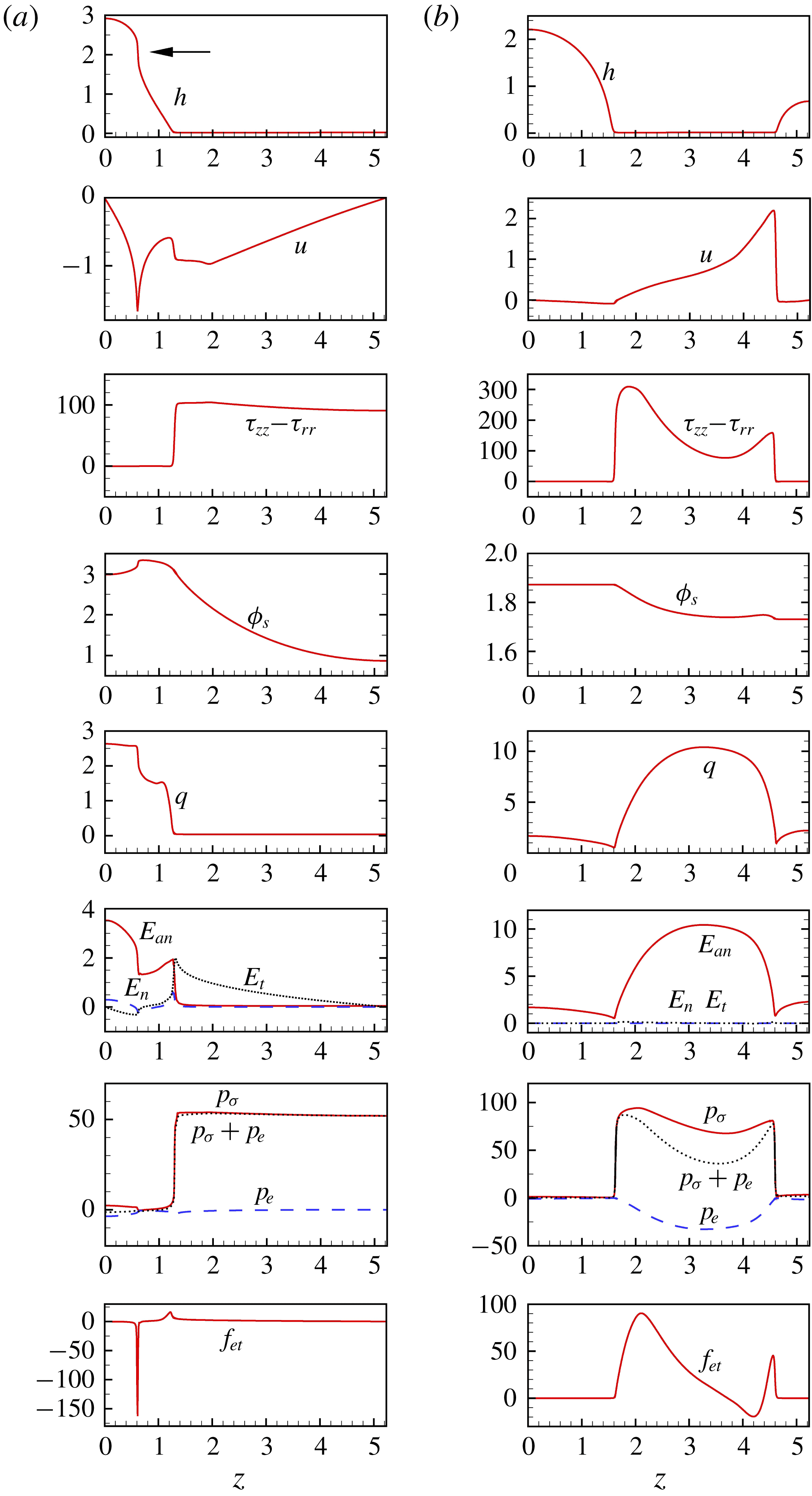
Schematic of the experimental set-up.

Formation of spike structure on the liquid jet of ethanol at electric voltage 6.3 kV and flow rate
 $2500~\unicode[STIX]{x03BC}\text{l}~\text{min}^{-1}$
.

Formation of spike structure on the liquid jet of a mixture of ethanol and glycerol at electric voltage 6.4 kV and flow rate 3000
 $\unicode[STIX]{x03BC}\text{l}~\text{min}^{-1}$
.

Four different liquids are tested in the experiment: distilled water (small viscosity and large surface tension), ethanol (small viscosity and small surface tension), a mixture of ethanol and glycerol (large viscosity and small surface tension) and a slightly viscoelastic aqueous solution of polyethylene oxide (PEO, molecular weight
 $2\times 10^{6}$
). As shown in figures 13 and 14, for ethanol or the ethanol–glycerol mixture, whose surface tension is small, when an sufficiently large electric voltage is imposed on the jet, the continuous radial elongation of droplets and the resulting pointed spikes quite similar to those predicted by the 1-D model are observed in the experiment. However, for water or the viscoelastic PEO aqueous solution, whose surface tension is large, the formation of spikes is not observed, because corona discharge occurs before the electrostatic force is large enough to overcome the capillary force and trigger the occurrence of spikes. In the future we will conduct a systematic experimental study on spike structures.
Secondary break-up of a spike with the emission of tens of ultra-fine jets from its periphery.

In addition, an interesting phenomenon observed in the experiment is the secondary break-up of a spike occurring at its periphery, as illustrated in figures (13) and (14). Also note that, prior to this secondary break-up, the spike may be fully elongated in the radial direction and develop an extremely oblate configuration, which is possibly due to the radial flow in it. A close-up in figure 15 clearly shows that tens of fine jets are emitted from the periphery of the spike. These jets undergo the Rayleigh instability and are expected to break up into super-small droplets ultimately, although the details of break-up and the resulting droplets are indiscernible in the figure due to the poor resolution. The second break-up of the spike structure and the subsequent atomization is apparently three-dimensional and cannot be predicted by a simplified 1-D model. It is of interest to study theoretically and experimentally this instability as well as the effect of the relevant factors including inertia, electric field and viscoelasticity on it. Many open problems remain in the formation and subsequent break-up of the spike structure.
5 Conclusion
In this work a 1-D model is built to numerically study the nonlinear dynamics of an electrically charged viscoelastic liquid jet of finite conductivity. The effect of the charge level, axial wavenumber and finite conductivity on the nonlinear behaviour of the viscoelastic jet is explored. Four different structures, i.e. the beads-on-a-string structure with satellite droplets, the beads-on-a-string structure with no satellite droplets, the quasi-spike structure and the spike structure, are identified. At small charge levels, the perturbed jet evolves into a quasistatic beads-on-a-string structure with satellite droplets at small wavenumbers and with no satellites at large wavenumbers; at large charge levels, an unstable quasi-spike or spike structure is formed. The quasi-spike structure occurs only in the finite conductivity case, in which the non-zero tangential electrostatic force is responsible for its formation. The tangential electrostatic force also plays a role in the formation of the beads-on-a-string and the spike structures: for the former, it hinders the thinning of the filament; for the latter, it accelerates the formation of spikes at the late stages. Finite conductivity may also decrease the size of satellite droplets in the beads-on-a-string structure and leads to the transition from beads-on-a-string to quasi-spike structure. In the finite conductivity case the thinning of the filament in the beads-on-a-string structure deviates little from the
 $1/3De$
exponential law of non-electrified viscoelastic jets. A comparison between the finite conductivity and large conductivity cases is made. It is found that, in the large conductivity case, the axial non-uniformity of the forces, including the first normal stress difference, the capillary pressure, the electrostatic pressure and the tangential electrical force are remarkable, whereas in the finite conductivity case their distributions are almost uniform in the filament. In addition, a preliminary experiment is carried out to observe spikes. The spike structure captured in the experiment is similar in appearance to that predicted by the 1-D model.
Under the slender body approximation, the flow field is simplified in the present 1-D model. On the other hand, the experimental result proves that when the deformation of the droplets gets large, the 2-D effect becomes significant, and in such a case the use of the 1-D model inevitably introduces inaccuracy. The actual 2-D motion of the liquid at large deformations is of particular interest. To test the validity of the 1-D model and to explore the 2-D nonlinear dynamics of electrically charged viscoelastic liquid jets, a robust 2-D algorithm needs to be developed.
Acknowledgements
This work was supported by the National Natural Science Foundation of China, project nos 11772328 and 11621202. We thank all the reviewers for their helpful comments and constructive suggestions.
Appendix A. The derivation of the 1-D equations
Considering symmetry, in the cylindrical coordinate system, the continuity equation is
 $$\begin{eqnarray}\displaystyle {\displaystyle \frac{1}{r}}{\displaystyle \frac{\unicode[STIX]{x2202}}{\unicode[STIX]{x2202}r}}(rv)+{\displaystyle \frac{\unicode[STIX]{x2202}u}{\unicode[STIX]{x2202}z}}=0, & & \displaystyle\end{eqnarray}$$
the momentum equation in the radial direction is
 $$\begin{eqnarray}\displaystyle \unicode[STIX]{x1D70C}\left({\displaystyle \frac{\unicode[STIX]{x2202}v}{\unicode[STIX]{x2202}t}}+v{\displaystyle \frac{\unicode[STIX]{x2202}v}{\unicode[STIX]{x2202}r}}+u{\displaystyle \frac{\unicode[STIX]{x2202}v}{\unicode[STIX]{x2202}z}}\right) & = & \displaystyle -{\displaystyle \frac{\unicode[STIX]{x2202}p}{\unicode[STIX]{x2202}r}}+\unicode[STIX]{x1D702}_{s}\left({\displaystyle \frac{\unicode[STIX]{x2202}^{2}v}{\unicode[STIX]{x2202}r^{2}}}+{\displaystyle \frac{1}{r}}{\displaystyle \frac{\unicode[STIX]{x2202}v}{\unicode[STIX]{x2202}r}}-{\displaystyle \frac{v}{r^{2}}}+{\displaystyle \frac{\unicode[STIX]{x2202}^{2}v}{\unicode[STIX]{x2202}z^{2}}}\right)\nonumber\\ \displaystyle & & \displaystyle +\,{\displaystyle \frac{\unicode[STIX]{x2202}\unicode[STIX]{x1D70F}_{rr}}{\unicode[STIX]{x2202}r}}+{\displaystyle \frac{\unicode[STIX]{x2202}\unicode[STIX]{x1D70F}_{rz}}{\unicode[STIX]{x2202}z}}+{\displaystyle \frac{\unicode[STIX]{x1D70F}_{rr}-\unicode[STIX]{x1D70F}_{\unicode[STIX]{x1D703}\unicode[STIX]{x1D703}}}{r}},\end{eqnarray}$$
where
 $\unicode[STIX]{x1D70F}_{rz}$
and
 $\unicode[STIX]{x1D70F}_{\unicode[STIX]{x1D703}\unicode[STIX]{x1D703}}$
are the
 $rz-$
and
 $\unicode[STIX]{x1D703}\unicode[STIX]{x1D703}-$
components of the polymeric stress tensor
 $\unicode[STIX]{x1D749}_{p}$
, respectively, and in the axial direction is
 $$\begin{eqnarray}\displaystyle \unicode[STIX]{x1D70C}\left({\displaystyle \frac{\unicode[STIX]{x2202}u}{\unicode[STIX]{x2202}t}}+v{\displaystyle \frac{\unicode[STIX]{x2202}u}{\unicode[STIX]{x2202}r}}+u{\displaystyle \frac{\unicode[STIX]{x2202}u}{\unicode[STIX]{x2202}z}}\right) & = & \displaystyle -{\displaystyle \frac{\unicode[STIX]{x2202}p}{\unicode[STIX]{x2202}z}}+\unicode[STIX]{x1D702}_{s}\left({\displaystyle \frac{\unicode[STIX]{x2202}^{2}u}{\unicode[STIX]{x2202}r^{2}}}+{\displaystyle \frac{1}{r}}{\displaystyle \frac{\unicode[STIX]{x2202}u}{\unicode[STIX]{x2202}r}}+{\displaystyle \frac{\unicode[STIX]{x2202}^{2}u}{\unicode[STIX]{x2202}z^{2}}}\right)\nonumber\\ \displaystyle & & \displaystyle +\,{\displaystyle \frac{\unicode[STIX]{x2202}\unicode[STIX]{x1D70F}_{rz}}{\unicode[STIX]{x2202}r}}+{\displaystyle \frac{\unicode[STIX]{x1D70F}_{rz}}{r}}+{\displaystyle \frac{\unicode[STIX]{x2202}\unicode[STIX]{x1D70F}_{zz}}{\unicode[STIX]{x2202}z}},\end{eqnarray}$$
and the constitutive equations for the polymeric stress components
 $\unicode[STIX]{x1D70F}_{rr}$
,
 $\unicode[STIX]{x1D70F}_{\unicode[STIX]{x1D703}\unicode[STIX]{x1D703}}$
,
 $\unicode[STIX]{x1D70F}_{zz}$
and
 $\unicode[STIX]{x1D70F}_{rz}$
are
 $$\begin{eqnarray}\displaystyle & \displaystyle \unicode[STIX]{x1D70F}_{rr}+\unicode[STIX]{x1D706}_{1}\left({\displaystyle \frac{\unicode[STIX]{x2202}\unicode[STIX]{x1D70F}_{rr}}{\unicode[STIX]{x2202}t}}+v{\displaystyle \frac{\unicode[STIX]{x2202}\unicode[STIX]{x1D70F}_{rr}}{\unicode[STIX]{x2202}r}}+u\frac{\unicode[STIX]{x2202}\unicode[STIX]{x1D70F}_{rr}}{\unicode[STIX]{x2202}z}-2\unicode[STIX]{x1D70F}_{rr}{\displaystyle \frac{\unicode[STIX]{x2202}v}{\unicode[STIX]{x2202}r}}-2\unicode[STIX]{x1D70F}_{rz}\frac{\unicode[STIX]{x2202}v}{\unicode[STIX]{x2202}z}\right)=2\unicode[STIX]{x1D702}_{p}{\displaystyle \frac{\unicode[STIX]{x2202}v}{\unicode[STIX]{x2202}r}}, & \displaystyle\end{eqnarray}$$
 $$\begin{eqnarray}\displaystyle & \displaystyle \unicode[STIX]{x1D70F}_{\unicode[STIX]{x1D703}\unicode[STIX]{x1D703}}+\unicode[STIX]{x1D706}_{1}\left({\displaystyle \frac{\unicode[STIX]{x2202}\unicode[STIX]{x1D70F}_{\unicode[STIX]{x1D703}\unicode[STIX]{x1D703}}}{\unicode[STIX]{x2202}t}}+v{\displaystyle \frac{\unicode[STIX]{x2202}\unicode[STIX]{x1D70F}_{\unicode[STIX]{x1D703}\unicode[STIX]{x1D703}}}{\unicode[STIX]{x2202}r}}+u{\displaystyle \frac{\unicode[STIX]{x2202}\unicode[STIX]{x1D70F}_{\unicode[STIX]{x1D703}\unicode[STIX]{x1D703}}}{\unicode[STIX]{x2202}z}}-{\displaystyle \frac{2v}{r}}\unicode[STIX]{x1D70F}_{\unicode[STIX]{x1D703}\unicode[STIX]{x1D703}}\right)=2\unicode[STIX]{x1D702}_{p}{\displaystyle \frac{v}{r}}, & \displaystyle\end{eqnarray}$$
 $$\begin{eqnarray}\displaystyle & \displaystyle \unicode[STIX]{x1D70F}_{zz}+\unicode[STIX]{x1D706}_{1}\left({\displaystyle \frac{\unicode[STIX]{x2202}\unicode[STIX]{x1D70F}_{zz}}{\unicode[STIX]{x2202}t}}+v{\displaystyle \frac{\unicode[STIX]{x2202}\unicode[STIX]{x1D70F}_{zz}}{\unicode[STIX]{x2202}r}}+u{\displaystyle \frac{\unicode[STIX]{x2202}\unicode[STIX]{x1D70F}_{zz}}{\unicode[STIX]{x2202}z}}-2\unicode[STIX]{x1D70F}_{rz}{\displaystyle \frac{\unicode[STIX]{x2202}u}{\unicode[STIX]{x2202}r}}-2\unicode[STIX]{x1D70F}_{zz}{\displaystyle \frac{\unicode[STIX]{x2202}u}{\unicode[STIX]{x2202}z}}\right)=2\unicode[STIX]{x1D702}_{p}{\displaystyle \frac{\unicode[STIX]{x2202}u}{\unicode[STIX]{x2202}z}}, & \displaystyle\end{eqnarray}$$
 $$\begin{eqnarray}\displaystyle & \displaystyle \unicode[STIX]{x1D70F}_{rz}+\unicode[STIX]{x1D706}_{1}\left({\displaystyle \frac{\unicode[STIX]{x2202}\unicode[STIX]{x1D70F}_{rz}}{\unicode[STIX]{x2202}t}}+v{\displaystyle \frac{\unicode[STIX]{x2202}\unicode[STIX]{x1D70F}_{rz}}{\unicode[STIX]{x2202}r}}+u{\displaystyle \frac{\unicode[STIX]{x2202}\unicode[STIX]{x1D70F}_{rz}}{\unicode[STIX]{x2202}z}}+{\displaystyle \frac{\unicode[STIX]{x1D70F}_{rz}v}{r}}-\unicode[STIX]{x1D70F}_{rr}{\displaystyle \frac{\unicode[STIX]{x2202}u}{\unicode[STIX]{x2202}r}}-\unicode[STIX]{x1D70F}_{zz}{\displaystyle \frac{\unicode[STIX]{x2202}v}{\unicode[STIX]{x2202}z}}\right)=\unicode[STIX]{x1D702}_{p}\left({\displaystyle \frac{\unicode[STIX]{x2202}v}{\unicode[STIX]{x2202}z}}+{\displaystyle \frac{\unicode[STIX]{x2202}u}{\unicode[STIX]{x2202}r}}\right). & \displaystyle\end{eqnarray}$$
The kinematic boundary condition at the jet surface
 $r=h(z,t)$
is
 $$\begin{eqnarray}\displaystyle v={\displaystyle \frac{\unicode[STIX]{x2202}h}{\unicode[STIX]{x2202}t}}+u{\displaystyle \frac{\unicode[STIX]{x2202}h}{\unicode[STIX]{x2202}z}}, & & \displaystyle\end{eqnarray}$$
and the normal and tangential dynamic boundary conditions are
 $$\begin{eqnarray}\displaystyle p & = & \displaystyle -\frac{1}{2}\left[\unicode[STIX]{x1D700}_{a}(E_{an}^{2}-E_{t}^{2})-\unicode[STIX]{x1D700}(E_{n}^{2}-E_{t}^{2})\right]+\unicode[STIX]{x1D70E}\unicode[STIX]{x1D735}\boldsymbol{\cdot }\boldsymbol{n}+{\displaystyle \frac{1}{1+\left({\displaystyle \frac{\unicode[STIX]{x2202}h}{\unicode[STIX]{x2202}z}}\right)^{2}}}\nonumber\\ \displaystyle & & \displaystyle \times \left[2\unicode[STIX]{x1D702}_{s}{\displaystyle \frac{\unicode[STIX]{x2202}v}{\unicode[STIX]{x2202}r}}+\unicode[STIX]{x1D70F}_{rr}+\left({\displaystyle \frac{\unicode[STIX]{x2202}h}{\unicode[STIX]{x2202}z}}\right)^{2}\left(2\unicode[STIX]{x1D702}_{s}{\displaystyle \frac{\unicode[STIX]{x2202}u}{\unicode[STIX]{x2202}z}}+\unicode[STIX]{x1D70F}_{zz}\right)-2{\displaystyle \frac{\unicode[STIX]{x2202}h}{\unicode[STIX]{x2202}z}}\left(\unicode[STIX]{x1D702}_{s}\left({\displaystyle \frac{\unicode[STIX]{x2202}v}{\unicode[STIX]{x2202}z}}+{\displaystyle \frac{\unicode[STIX]{x2202}u}{\unicode[STIX]{x2202}r}}\right)+\unicode[STIX]{x1D70F}_{rz}\right)\right],\quad \nonumber\\ \displaystyle & & \displaystyle\end{eqnarray}$$
and
 $$\begin{eqnarray}\displaystyle & & \displaystyle -E_{t}q\left[1+\left({\displaystyle \frac{\unicode[STIX]{x2202}h}{\unicode[STIX]{x2202}z}}\right)^{2}\right]+\left[\unicode[STIX]{x1D702}_{s}\left({\displaystyle \frac{\unicode[STIX]{x2202}v}{\unicode[STIX]{x2202}z}}+{\displaystyle \frac{\unicode[STIX]{x2202}u}{\unicode[STIX]{x2202}r}}\right)+\unicode[STIX]{x1D70F}_{rz}\right]\left[1-\left({\displaystyle \frac{\unicode[STIX]{x2202}h}{\unicode[STIX]{x2202}z}}\right)^{2}\right]\nonumber\\ \displaystyle & & \displaystyle \qquad +\,{\displaystyle \frac{\unicode[STIX]{x2202}h}{\unicode[STIX]{x2202}z}}\left(2\unicode[STIX]{x1D702}_{s}{\displaystyle \frac{\unicode[STIX]{x2202}v}{\unicode[STIX]{x2202}r}}+\unicode[STIX]{x1D70F}_{rr}-2\unicode[STIX]{x1D702}_{s}{\displaystyle \frac{\unicode[STIX]{x2202}u}{\unicode[STIX]{x2202}z}}-\unicode[STIX]{x1D70F}_{zz}\right)=0,\end{eqnarray}$$
respectively.
An alternative form of the surface charge conservation equation is
 $$\begin{eqnarray}\displaystyle {\displaystyle \frac{\unicode[STIX]{x2202}q}{\unicode[STIX]{x2202}t}}+\boldsymbol{v}\boldsymbol{\cdot }\unicode[STIX]{x1D6FB}_{s}q-q\boldsymbol{n}\boldsymbol{\cdot }(\boldsymbol{n}\boldsymbol{\cdot }\unicode[STIX]{x1D735})\boldsymbol{v}-KE_{n}=0. & & \displaystyle\end{eqnarray}$$
Let
 $\ell _{r}$
be the typical thickness and
 $\ell _{z}$
be the typical axial length of the perturbed liquid jet. When the jet is a slender body,
 $\ell _{r}$
is much smaller than
 $\ell _{z}$
, that is,
 $$\begin{eqnarray}\displaystyle \ell _{r}=\unicode[STIX]{x1D716}\ell _{z}, & & \displaystyle\end{eqnarray}$$
where
 $\unicode[STIX]{x1D716}$
is a small parameter. Let
 $\unicode[STIX]{x1D717}$
be the typical time scale. In this problem, the balance of inertia, surface tension, viscoelastic and electrostatic forces indicates that (Eggers & Villermaux Reference Eggers and Villermaux2008)
 $$\begin{eqnarray}\displaystyle \unicode[STIX]{x1D702}_{0}\approx \unicode[STIX]{x1D70C}\ell _{z}^{2}/\unicode[STIX]{x1D717},\quad \unicode[STIX]{x1D70E}\approx \unicode[STIX]{x1D70C}\ell _{r}\ell _{z}^{2}/\unicode[STIX]{x1D717}^{2},\quad \unicode[STIX]{x1D706}_{1}\approx \unicode[STIX]{x1D717},\quad Q_{0}^{2}/\unicode[STIX]{x1D700}_{a}\approx \ell _{z}^{2}/\unicode[STIX]{x1D717}^{2}, & & \displaystyle\end{eqnarray}$$
and
 $$\begin{eqnarray}\displaystyle \ell _{z}\approx \unicode[STIX]{x1D716}\ell _{\unicode[STIX]{x1D708}},~\ell _{r}\approx \unicode[STIX]{x1D716}^{2}\ell _{\unicode[STIX]{x1D708}},\quad \unicode[STIX]{x1D717}\approx \unicode[STIX]{x1D716}^{2}t_{\unicode[STIX]{x1D708}}, & & \displaystyle\end{eqnarray}$$
where
 $\ell _{v}=\unicode[STIX]{x1D702}_{0}^{2}/\unicode[STIX]{x1D70C}\unicode[STIX]{x1D70E}$
and
 $t_{\unicode[STIX]{x1D708}}=\unicode[STIX]{x1D702}_{0}^{3}/\unicode[STIX]{x1D70C}\unicode[STIX]{x1D70E}^{2}$
.
Using
 $\ell _{r}$
,
 $\ell _{z}$
and
 $\unicode[STIX]{x1D717}$
to non-dimensionalize the quantities, gives
 $$\begin{eqnarray}\displaystyle \left.\begin{array}{@{}c@{}}r=\ell _{r}\tilde{r},\quad z=\ell _{z}\tilde{z},\quad t=\unicode[STIX]{x1D717}\tilde{t},\quad h=\ell _{r}\tilde{h},\quad v=\frac{\ell _{r}}{\unicode[STIX]{x1D717}}\tilde{v},\quad u={\displaystyle \frac{\ell _{z}}{\unicode[STIX]{x1D717}}}\tilde{u} ,\\ p={\displaystyle \frac{\unicode[STIX]{x1D70C}\ell _{z}^{2}}{\unicode[STIX]{x1D717}^{2}}}\tilde{p},\quad \unicode[STIX]{x1D70F}_{rr}={\displaystyle \frac{\unicode[STIX]{x1D70C}\ell _{z}^{2}}{\unicode[STIX]{x1D717}^{2}}}\tilde{\unicode[STIX]{x1D70F}}_{rr},\quad \unicode[STIX]{x1D70F}_{\unicode[STIX]{x1D703}\unicode[STIX]{x1D703}}={\displaystyle \frac{\unicode[STIX]{x1D70C}\ell _{z}^{2}}{\unicode[STIX]{x1D717}^{2}}}\tilde{\unicode[STIX]{x1D70F}}_{\unicode[STIX]{x1D703}\unicode[STIX]{x1D703}},\quad \unicode[STIX]{x1D70F}_{zz}={\displaystyle \frac{\unicode[STIX]{x1D70C}\ell _{z}^{2}}{\unicode[STIX]{x1D717}^{2}}}\tilde{\unicode[STIX]{x1D70F}}_{zz},\quad \unicode[STIX]{x1D70F}_{rz}={\displaystyle \frac{\unicode[STIX]{x1D70C}\ell _{z}^{3}}{\unicode[STIX]{x1D717}^{2}\ell _{r}}}\tilde{\unicode[STIX]{x1D70F}}_{rz},\end{array}\right\}\quad & & \displaystyle\end{eqnarray}$$
where the tilde denotes the corresponding non-dimensional quantities. In addition, the quantities related to the electric field are non-dimensionalized by
 $Q_{0}$
and
 $\unicode[STIX]{x1D700}_{a}$
, i.e.
 $$\begin{eqnarray}\displaystyle E_{an}={\displaystyle \frac{Q_{0}}{\unicode[STIX]{x1D700}_{a}}}\tilde{E}_{an},\quad E_{n}={\displaystyle \frac{Q_{0}}{\unicode[STIX]{x1D700}_{a}}}\tilde{E}_{n},\quad E_{t}={\displaystyle \frac{Q_{0}}{\unicode[STIX]{x1D700}_{a}}}{\displaystyle \frac{\ell _{r}}{\ell _{z}}}\tilde{E}_{t},\quad q=Q_{0}\tilde{q}. & & \displaystyle\end{eqnarray}$$
Hence the non-dimensionalized governing equations are expressed as
 $$\begin{eqnarray}\displaystyle {\displaystyle \frac{\unicode[STIX]{x2202}\tilde{v}}{\unicode[STIX]{x2202}\tilde{r}}}+{\displaystyle \frac{\tilde{v}}{\tilde{r}}}+{\displaystyle \frac{\unicode[STIX]{x2202}\tilde{u} }{\unicode[STIX]{x2202}\tilde{z}}}=0, & & \displaystyle\end{eqnarray}$$
 $$\begin{eqnarray}\displaystyle {\displaystyle \frac{\unicode[STIX]{x2202}\tilde{v}}{\unicode[STIX]{x2202}\tilde{t}}}+\tilde{v}{\displaystyle \frac{\unicode[STIX]{x2202}\tilde{v}}{\unicode[STIX]{x2202}\tilde{r}}}+\tilde{u} \frac{\unicode[STIX]{x2202}\tilde{v}}{\unicode[STIX]{x2202}\tilde{z}} & = & \displaystyle -{\displaystyle \frac{1}{\unicode[STIX]{x1D716}^{2}}}{\displaystyle \frac{\unicode[STIX]{x2202}\tilde{p}}{\unicode[STIX]{x2202}\tilde{r}}}+\unicode[STIX]{x1D6FD}{\displaystyle \frac{1}{\unicode[STIX]{x1D716}^{2}}}\left({\displaystyle \frac{\unicode[STIX]{x2202}^{2}\tilde{v}}{\unicode[STIX]{x2202}\tilde{r}^{2}}}+{\displaystyle \frac{1}{\tilde{r}}}\frac{\unicode[STIX]{x2202}\tilde{v}}{\unicode[STIX]{x2202}\tilde{r}}-{\displaystyle \frac{\tilde{v}}{\tilde{r}^{2}}}\right)+\unicode[STIX]{x1D6FD}{\displaystyle \frac{\unicode[STIX]{x2202}^{2}\tilde{v}}{\unicode[STIX]{x2202}\tilde{z}^{2}}}\nonumber\\ \displaystyle & & \displaystyle +\,{\displaystyle \frac{1}{\unicode[STIX]{x1D716}^{2}}}{\displaystyle \frac{\unicode[STIX]{x2202}\tilde{\unicode[STIX]{x1D70F}}_{rr}}{\unicode[STIX]{x2202}\tilde{r}}}+{\displaystyle \frac{1}{\unicode[STIX]{x1D716}^{2}}}{\displaystyle \frac{\unicode[STIX]{x2202}\tilde{\unicode[STIX]{x1D70F}}_{rz}}{\unicode[STIX]{x2202}\tilde{z}}}+{\displaystyle \frac{1}{\unicode[STIX]{x1D716}^{2}}}{\displaystyle \frac{\tilde{\unicode[STIX]{x1D70F}}_{rr}-\tilde{\unicode[STIX]{x1D70F}}_{\unicode[STIX]{x1D703}\unicode[STIX]{x1D703}}}{\tilde{r}}},\end{eqnarray}$$
 $$\begin{eqnarray}\displaystyle {\displaystyle \frac{\unicode[STIX]{x2202}\tilde{u} }{\unicode[STIX]{x2202}\tilde{t}}}+\tilde{v}{\displaystyle \frac{\unicode[STIX]{x2202}\tilde{u} }{\unicode[STIX]{x2202}\tilde{r}}}+\tilde{u} {\displaystyle \frac{\unicode[STIX]{x2202}\tilde{u} }{\unicode[STIX]{x2202}\tilde{z}}} & = & \displaystyle -{\displaystyle \frac{\unicode[STIX]{x2202}\tilde{p}}{\unicode[STIX]{x2202}\tilde{z}}}+\unicode[STIX]{x1D6FD}{\displaystyle \frac{1}{\unicode[STIX]{x1D716}^{2}}}\left({\displaystyle \frac{\unicode[STIX]{x2202}^{2}\tilde{u} }{\unicode[STIX]{x2202}\tilde{r}^{2}}}+{\displaystyle \frac{1}{\tilde{r}}}{\displaystyle \frac{\unicode[STIX]{x2202}\tilde{u} }{\unicode[STIX]{x2202}\tilde{r}}}\right)+\unicode[STIX]{x1D6FD}{\displaystyle \frac{\unicode[STIX]{x2202}^{2}\tilde{u} }{\unicode[STIX]{x2202}\tilde{z}^{2}}}\nonumber\\ \displaystyle & & \displaystyle +\,{\displaystyle \frac{1}{\unicode[STIX]{x1D716}^{2}}}{\displaystyle \frac{\unicode[STIX]{x2202}\tilde{\unicode[STIX]{x1D70F}}_{rz}}{\unicode[STIX]{x2202}\tilde{r}}}+{\displaystyle \frac{1}{\unicode[STIX]{x1D716}^{2}}}{\displaystyle \frac{\tilde{\unicode[STIX]{x1D70F}}_{rz}}{\tilde{r}}}+{\displaystyle \frac{\unicode[STIX]{x2202}\tilde{\unicode[STIX]{x1D70F}}_{zz}}{\unicode[STIX]{x2202}\tilde{z}}},\end{eqnarray}$$
 $$\begin{eqnarray}\displaystyle & \displaystyle \tilde{\unicode[STIX]{x1D70F}}_{rr}+{\displaystyle \frac{\unicode[STIX]{x2202}\tilde{\unicode[STIX]{x1D70F}}_{rr}}{\unicode[STIX]{x2202}\tilde{t}}}+\tilde{v}{\displaystyle \frac{\unicode[STIX]{x2202}\tilde{\unicode[STIX]{x1D70F}}_{rr}}{\unicode[STIX]{x2202}\tilde{r}}}+\tilde{u} {\displaystyle \frac{\unicode[STIX]{x2202}\tilde{\unicode[STIX]{x1D70F}}_{rr}}{\unicode[STIX]{x2202}\tilde{z}}}-2\tilde{\unicode[STIX]{x1D70F}}_{rr}{\displaystyle \frac{\unicode[STIX]{x2202}\tilde{v}}{\unicode[STIX]{x2202}\tilde{r}}}-2\tilde{\unicode[STIX]{x1D70F}}_{rz}{\displaystyle \frac{\unicode[STIX]{x2202}\tilde{v}}{\unicode[STIX]{x2202}\tilde{z}}}=2(1-\unicode[STIX]{x1D6FD}){\displaystyle \frac{\unicode[STIX]{x2202}\tilde{v}}{\unicode[STIX]{x2202}\tilde{r}}}, & \displaystyle\end{eqnarray}$$
 $$\begin{eqnarray}\displaystyle & \displaystyle \tilde{\unicode[STIX]{x1D70F}}_{\unicode[STIX]{x1D703}\unicode[STIX]{x1D703}}+{\displaystyle \frac{\unicode[STIX]{x2202}\tilde{\unicode[STIX]{x1D70F}}_{\unicode[STIX]{x1D703}\unicode[STIX]{x1D703}}}{\unicode[STIX]{x2202}\tilde{t}}}+\tilde{v}{\displaystyle \frac{\unicode[STIX]{x2202}\tilde{\unicode[STIX]{x1D70F}}_{\unicode[STIX]{x1D703}\unicode[STIX]{x1D703}}}{\unicode[STIX]{x2202}\tilde{r}}}+\tilde{u} {\displaystyle \frac{\unicode[STIX]{x2202}\tilde{\unicode[STIX]{x1D70F}}_{\unicode[STIX]{x1D703}\unicode[STIX]{x1D703}}}{\unicode[STIX]{x2202}\tilde{z}}}-{\displaystyle \frac{2\tilde{v}}{\tilde{r}}}\tilde{\unicode[STIX]{x1D70F}}_{\unicode[STIX]{x1D703}\unicode[STIX]{x1D703}}=2(1-\unicode[STIX]{x1D6FD}){\displaystyle \frac{\tilde{v}}{\tilde{r}}}, & \displaystyle\end{eqnarray}$$
 $$\begin{eqnarray}\displaystyle & \displaystyle \tilde{\unicode[STIX]{x1D70F}}_{zz}+{\displaystyle \frac{\unicode[STIX]{x2202}\tilde{\unicode[STIX]{x1D70F}}_{zz}}{\unicode[STIX]{x2202}\tilde{t}}}+\tilde{v}{\displaystyle \frac{\unicode[STIX]{x2202}\tilde{\unicode[STIX]{x1D70F}}_{zz}}{\unicode[STIX]{x2202}\tilde{r}}}+\tilde{u} {\displaystyle \frac{\unicode[STIX]{x2202}\tilde{\unicode[STIX]{x1D70F}}_{zz}}{\unicode[STIX]{x2202}\tilde{z}}}-2{\displaystyle \frac{1}{\unicode[STIX]{x1D716}^{2}}}\tilde{\unicode[STIX]{x1D70F}}_{rz}{\displaystyle \frac{\unicode[STIX]{x2202}\tilde{u} }{\unicode[STIX]{x2202}\tilde{r}}}-2\tilde{\unicode[STIX]{x1D70F}}_{zz}{\displaystyle \frac{\unicode[STIX]{x2202}\tilde{u} }{\unicode[STIX]{x2202}\tilde{z}}}=2(1-\unicode[STIX]{x1D6FD}){\displaystyle \frac{\unicode[STIX]{x2202}\tilde{u} }{\unicode[STIX]{x2202}\tilde{z}}}, & \displaystyle\end{eqnarray}$$
 $$\begin{eqnarray}\displaystyle & \displaystyle \tilde{\unicode[STIX]{x1D70F}}_{rz}+{\displaystyle \frac{\unicode[STIX]{x2202}\tilde{\unicode[STIX]{x1D70F}}_{rz}}{\unicode[STIX]{x2202}\tilde{t}}}+\tilde{v}{\displaystyle \frac{\unicode[STIX]{x2202}\tilde{\unicode[STIX]{x1D70F}}_{rz}}{\unicode[STIX]{x2202}\tilde{r}}}+\tilde{u} {\displaystyle \frac{\unicode[STIX]{x2202}\tilde{\unicode[STIX]{x1D70F}}_{rz}}{\unicode[STIX]{x2202}\tilde{z}}}+{\displaystyle \frac{\tilde{\unicode[STIX]{x1D70F}}_{rz}\tilde{v}}{\tilde{r}}}-\tilde{\unicode[STIX]{x1D70F}}_{rr}{\displaystyle \frac{\unicode[STIX]{x2202}\tilde{u} }{\unicode[STIX]{x2202}\tilde{r}}}-\unicode[STIX]{x1D716}^{2}\tilde{\unicode[STIX]{x1D70F}}_{zz}{\displaystyle \frac{\unicode[STIX]{x2202}\tilde{v}}{\unicode[STIX]{x2202}\tilde{z}}}=(1-\unicode[STIX]{x1D6FD})\left(\unicode[STIX]{x1D716}^{2}{\displaystyle \frac{\unicode[STIX]{x2202}\tilde{v}}{\unicode[STIX]{x2202}\tilde{z}}}+{\displaystyle \frac{\unicode[STIX]{x2202}\tilde{u} }{\unicode[STIX]{x2202}\tilde{r}}}\right),\quad & \displaystyle \nonumber\\ \displaystyle & & \displaystyle\end{eqnarray}$$
and the non-dimensionalized boundary conditions at the jet surface
 $\tilde{r}=\tilde{h}(\tilde{z},\tilde{t})$
are
 $$\begin{eqnarray}\displaystyle \tilde{v}={\displaystyle \frac{\unicode[STIX]{x2202}\tilde{h}}{\unicode[STIX]{x2202}\tilde{t}}}+\tilde{u} {\displaystyle \frac{\unicode[STIX]{x2202}\tilde{h}}{\unicode[STIX]{x2202}\tilde{z}}}, & & \displaystyle\end{eqnarray}$$
 $$\begin{eqnarray}\displaystyle \tilde{p} & = & \displaystyle -{\displaystyle \frac{1}{2}}\left[\left(\tilde{E}_{an}^{2}-\tilde{E}_{t}^{2}\right)-\unicode[STIX]{x1D700}_{r}\left(\tilde{E}_{n}^{2}-\tilde{E}_{t}^{2}\right)\right]+\tilde{\unicode[STIX]{x1D735}}\boldsymbol{\cdot }\tilde{\boldsymbol{n}}+\frac{1}{1+\unicode[STIX]{x1D716}^{2}\left({\displaystyle \frac{\unicode[STIX]{x2202}\tilde{h}}{\unicode[STIX]{x2202}\tilde{z}}}\right)^{2}}\nonumber\\ \displaystyle & & \displaystyle \times \,\left[2\unicode[STIX]{x1D6FD}{\displaystyle \frac{\unicode[STIX]{x2202}\tilde{v}}{\unicode[STIX]{x2202}\tilde{r}}}+\tilde{\unicode[STIX]{x1D70F}}_{rr}+\unicode[STIX]{x1D716}^{2}\left({\displaystyle \frac{\unicode[STIX]{x2202}\tilde{h}}{\unicode[STIX]{x2202}\tilde{z}}}\right)^{2}\left(2\unicode[STIX]{x1D6FD}{\displaystyle \frac{\unicode[STIX]{x2202}\tilde{u} }{\unicode[STIX]{x2202}\tilde{z}}}+\tilde{\unicode[STIX]{x1D70F}}_{zz}\right)-2{\displaystyle \frac{\unicode[STIX]{x2202}\tilde{h}}{\unicode[STIX]{x2202}\tilde{z}}}\left(\unicode[STIX]{x1D6FD}\left(\unicode[STIX]{x1D716}^{2}\frac{\unicode[STIX]{x2202}\tilde{v}}{\unicode[STIX]{x2202}\tilde{z}}+\frac{\unicode[STIX]{x2202}\tilde{u} }{\unicode[STIX]{x2202}\tilde{r}}\right)+\tilde{\unicode[STIX]{x1D70F}}_{rz}\right)\right],\nonumber\\ \displaystyle & & \displaystyle\end{eqnarray}$$
 $$\begin{eqnarray}\displaystyle & & \displaystyle -\tilde{E}_{t}\tilde{q}\left[1+\unicode[STIX]{x1D716}^{2}\left({\displaystyle \frac{\unicode[STIX]{x2202}\tilde{h}}{\unicode[STIX]{x2202}\tilde{z}}}\right)^{2}\right]+\left[\unicode[STIX]{x1D6FD}\left({\displaystyle \frac{\unicode[STIX]{x2202}\tilde{v}}{\unicode[STIX]{x2202}\tilde{z}}}+\frac{1}{\unicode[STIX]{x1D716}^{2}}{\displaystyle \frac{\unicode[STIX]{x2202}\tilde{u} }{\unicode[STIX]{x2202}\tilde{r}}}\right)+{\displaystyle \frac{1}{\unicode[STIX]{x1D716}^{2}}}\tilde{\unicode[STIX]{x1D70F}}_{rz}\right]\left[1-\unicode[STIX]{x1D716}^{2}\left({\displaystyle \frac{\unicode[STIX]{x2202}\tilde{h}}{\unicode[STIX]{x2202}\tilde{z}}}\right)^{2}\right]\nonumber\\ \displaystyle & & \displaystyle \qquad +\,{\displaystyle \frac{\unicode[STIX]{x2202}\tilde{h}}{\unicode[STIX]{x2202}\tilde{z}}}\left[2\unicode[STIX]{x1D6FD}{\displaystyle \frac{\unicode[STIX]{x2202}\tilde{v}}{\unicode[STIX]{x2202}\tilde{r}}}+\tilde{\unicode[STIX]{x1D70F}}_{rr}-2\unicode[STIX]{x1D6FD}{\displaystyle \frac{\unicode[STIX]{x2202}\tilde{u} }{\unicode[STIX]{x2202}\tilde{z}}}-\tilde{\unicode[STIX]{x1D70F}}_{zz}\right]=0,\end{eqnarray}$$
 $$\begin{eqnarray}\displaystyle {\displaystyle \frac{\unicode[STIX]{x2202}\tilde{q}}{\unicode[STIX]{x2202}\tilde{t}}}+\tilde{\boldsymbol{v}}\boldsymbol{\cdot }\tilde{\unicode[STIX]{x1D6FB}}_{s}\tilde{q}-\tilde{q}\tilde{\boldsymbol{n}}\boldsymbol{\cdot }(\tilde{\boldsymbol{n}}\boldsymbol{\cdot }\tilde{\unicode[STIX]{x1D735}})\tilde{\boldsymbol{v}}-\unicode[STIX]{x1D70F}\unicode[STIX]{x1D700}_{r}\tilde{E}_{n}=0. & & \displaystyle\end{eqnarray}$$
Under the slender body approximation, the quantities can be expanded into a Taylor series of the radial coordinate
 $\unicode[STIX]{x1D716}\tilde{r}$
as follows (Chang et al.
Reference Chang, Demekhin and Kalaidin1999; López-Herrera et al.
Reference López-Herrera, Gañán-Calvo and Perez-Saborid1999; Eggers & Villermaux Reference Eggers and Villermaux2008),
 $$\begin{eqnarray}\displaystyle \tilde{u} & = & \displaystyle \tilde{u} _{0}(\tilde{z},\tilde{t})+\tilde{u} _{2}(\tilde{z},\tilde{t})\frac{(\unicode[STIX]{x1D716}\tilde{r})^{2}}{2}+\cdots \,,\end{eqnarray}$$
 $$\begin{eqnarray}\displaystyle \unicode[STIX]{x1D716}\tilde{v} & = & \displaystyle -\frac{\unicode[STIX]{x2202}\tilde{u} _{0}}{\unicode[STIX]{x2202}\tilde{z}}(\tilde{z},\tilde{t})\frac{\unicode[STIX]{x1D716}\tilde{r}}{2}-{\displaystyle \frac{\unicode[STIX]{x2202}\tilde{u} _{2}}{\unicode[STIX]{x2202}\tilde{z}}}(\tilde{z},\tilde{t}){\displaystyle \frac{(\unicode[STIX]{x1D716}\tilde{r})^{3}}{8}}+\cdots \,,\end{eqnarray}$$
 $$\begin{eqnarray}\displaystyle \tilde{p} & = & \displaystyle \tilde{p}_{0}(\tilde{z},\tilde{t})+\tilde{p}_{2}(\tilde{z},\tilde{t})(\unicode[STIX]{x1D716}\tilde{r})^{2}+\cdots \,,\end{eqnarray}$$
 $$\begin{eqnarray}\displaystyle \tilde{\unicode[STIX]{x1D70F}}_{rr} & = & \displaystyle \tilde{\unicode[STIX]{x1D70F}}_{rr0}(\tilde{z},\tilde{t})+\tilde{\unicode[STIX]{x1D70F}}_{rr2}(\tilde{z},\tilde{t})(\unicode[STIX]{x1D716}\tilde{r})^{2}+\cdots \,,\end{eqnarray}$$
 $$\begin{eqnarray}\displaystyle \tilde{\unicode[STIX]{x1D70F}}_{\unicode[STIX]{x1D703}\unicode[STIX]{x1D703}} & = & \displaystyle \tilde{\unicode[STIX]{x1D70F}}_{\unicode[STIX]{x1D703}\unicode[STIX]{x1D703}0}(\tilde{z},\tilde{t})+\tilde{\unicode[STIX]{x1D70F}}_{\unicode[STIX]{x1D703}\unicode[STIX]{x1D703}2}(\tilde{z},\tilde{t})(\unicode[STIX]{x1D716}\tilde{r})^{2}+\cdots \,,\end{eqnarray}$$
 $$\begin{eqnarray}\displaystyle \tilde{\unicode[STIX]{x1D70F}}_{zz} & = & \displaystyle \tilde{\unicode[STIX]{x1D70F}}_{zz0}(\tilde{z},\tilde{t})+\tilde{\unicode[STIX]{x1D70F}}_{zz2}(\tilde{z},\tilde{t})(\unicode[STIX]{x1D716}\tilde{r})^{2}+\cdots \,,\end{eqnarray}$$
 $$\begin{eqnarray}\displaystyle \tilde{r}\tilde{\unicode[STIX]{x1D70F}}_{rz} & = & \displaystyle \tilde{\unicode[STIX]{x1D70F}}_{rz0}(\tilde{z},\tilde{t})+\tilde{\unicode[STIX]{x1D70F}}_{rz2}(\tilde{z},\tilde{t})(\unicode[STIX]{x1D716}\tilde{r})^{2}+\cdots \,.\end{eqnarray}$$
The above expansions of the velocity components
 $\tilde{u}$
and
 $\tilde{v}$
automatically satisfy the continuity equation (A 17). Substituting the expansions (A 28)–(A 34) into (A 18)–(A 27) and keeping only those leading-order terms yields
 $$\begin{eqnarray}\displaystyle & \displaystyle \tilde{\unicode[STIX]{x1D70F}}_{rr0}=\tilde{\unicode[STIX]{x1D70F}}_{\unicode[STIX]{x1D703}\unicode[STIX]{x1D703}0},~\tilde{\unicode[STIX]{x1D70F}}_{rz0}=0, & \displaystyle\end{eqnarray}$$
 $$\begin{eqnarray}\displaystyle & \displaystyle {\displaystyle \frac{\unicode[STIX]{x2202}\tilde{u} _{0}}{\unicode[STIX]{x2202}\tilde{t}}}+\tilde{u} _{0}{\displaystyle \frac{\unicode[STIX]{x2202}\tilde{u} _{0}}{\unicode[STIX]{x2202}\tilde{z}}}=-{\displaystyle \frac{\unicode[STIX]{x2202}\tilde{p}_{0}}{\unicode[STIX]{x2202}\tilde{z}}}+\unicode[STIX]{x1D6FD}\left(2\tilde{u} _{2}+{\displaystyle \frac{\unicode[STIX]{x2202}^{2}\tilde{u} _{0}}{\unicode[STIX]{x2202}\tilde{z}^{2}}}\right)+2\tilde{\unicode[STIX]{x1D70F}}_{rz2}+\frac{\unicode[STIX]{x2202}\tilde{\unicode[STIX]{x1D70F}}_{zz0}}{\unicode[STIX]{x2202}\tilde{z}}, & \displaystyle\end{eqnarray}$$
 $$\begin{eqnarray}\displaystyle & \displaystyle \tilde{\unicode[STIX]{x1D70F}}_{rr0}+{\displaystyle \frac{\unicode[STIX]{x2202}\tilde{\unicode[STIX]{x1D70F}}_{rr0}}{\unicode[STIX]{x2202}\tilde{t}}}+\tilde{u} _{0}{\displaystyle \frac{\unicode[STIX]{x2202}\tilde{\unicode[STIX]{x1D70F}}_{rr0}}{\unicode[STIX]{x2202}\tilde{z}}}+\tilde{\unicode[STIX]{x1D70F}}_{rr0}{\displaystyle \frac{\unicode[STIX]{x2202}\tilde{u} _{0}}{\unicode[STIX]{x2202}\tilde{z}}}=-\left(1-\unicode[STIX]{x1D6FD}\right)\frac{\unicode[STIX]{x2202}\tilde{u} _{0}}{\unicode[STIX]{x2202}\tilde{z}}, & \displaystyle\end{eqnarray}$$
 $$\begin{eqnarray}\displaystyle & \displaystyle \tilde{\unicode[STIX]{x1D70F}}_{\unicode[STIX]{x1D703}\unicode[STIX]{x1D703}0}+\frac{\unicode[STIX]{x2202}\tilde{\unicode[STIX]{x1D70F}}_{\unicode[STIX]{x1D703}\unicode[STIX]{x1D703}0}}{\unicode[STIX]{x2202}\tilde{t}}+\tilde{u} _{0}\frac{\unicode[STIX]{x2202}\tilde{\unicode[STIX]{x1D70F}}_{\unicode[STIX]{x1D703}\unicode[STIX]{x1D703}0}}{\unicode[STIX]{x2202}\tilde{z}}+\tilde{\unicode[STIX]{x1D70F}}_{\unicode[STIX]{x1D703}\unicode[STIX]{x1D703}0}\frac{\unicode[STIX]{x2202}\tilde{u} _{0}}{\unicode[STIX]{x2202}\tilde{z}}=-\left(1-\unicode[STIX]{x1D6FD}\right)\frac{\unicode[STIX]{x2202}\tilde{u} _{0}}{\unicode[STIX]{x2202}\tilde{z}}, & \displaystyle\end{eqnarray}$$
 $$\begin{eqnarray}\displaystyle & \displaystyle \tilde{\unicode[STIX]{x1D70F}}_{zz0}+{\displaystyle \frac{\unicode[STIX]{x2202}\tilde{\unicode[STIX]{x1D70F}}_{zz0}}{\unicode[STIX]{x2202}\tilde{t}}}+\tilde{u} _{0}{\displaystyle \frac{\unicode[STIX]{x2202}\tilde{\unicode[STIX]{x1D70F}}_{zz0}}{\unicode[STIX]{x2202}\tilde{z}}}-2\tilde{\unicode[STIX]{x1D70F}}_{zz0}{\displaystyle \frac{\unicode[STIX]{x2202}\tilde{u} _{0}}{\unicode[STIX]{x2202}\tilde{z}}}=2(1-\unicode[STIX]{x1D6FD}){\displaystyle \frac{\unicode[STIX]{x2202}\tilde{u} _{0}}{\unicode[STIX]{x2202}\tilde{z}}}, & \displaystyle\end{eqnarray}$$
 $$\begin{eqnarray}\displaystyle & & \displaystyle \tilde{\unicode[STIX]{x1D70F}}_{rz2}+{\displaystyle \frac{\unicode[STIX]{x2202}\tilde{\unicode[STIX]{x1D70F}}_{rz2}}{\unicode[STIX]{x2202}\tilde{t}}}-\tilde{\unicode[STIX]{x1D70F}}_{rz2}{\displaystyle \frac{\unicode[STIX]{x2202}\tilde{u} _{0}}{\unicode[STIX]{x2202}\tilde{z}}}+\tilde{u} _{0}\frac{\unicode[STIX]{x2202}\tilde{\unicode[STIX]{x1D70F}}_{rz2}}{\unicode[STIX]{x2202}\tilde{z}}-\tilde{\unicode[STIX]{x1D70F}}_{rr0}\tilde{u} _{2}+{\displaystyle \frac{1}{2}}\tilde{\unicode[STIX]{x1D70F}}_{zz0}{\displaystyle \frac{\unicode[STIX]{x2202}^{2}\tilde{u} _{0}}{\unicode[STIX]{x2202}\tilde{z}^{2}}}\nonumber\\ \displaystyle & & \displaystyle \quad =(1-\unicode[STIX]{x1D6FD})\left(\tilde{u} _{2}-{\displaystyle \frac{1}{2}}{\displaystyle \frac{\unicode[STIX]{x2202}^{2}\tilde{u} _{0}}{\unicode[STIX]{x2202}\tilde{z}^{2}}}\right),\end{eqnarray}$$
 $$\begin{eqnarray}\displaystyle & \displaystyle {\displaystyle \frac{\unicode[STIX]{x2202}\tilde{h}}{\unicode[STIX]{x2202}\tilde{t}}}+\tilde{u} _{0}{\displaystyle \frac{\unicode[STIX]{x2202}\tilde{h}}{\unicode[STIX]{x2202}\tilde{z}}}=-{\displaystyle \frac{\tilde{h}}{2}}{\displaystyle \frac{\unicode[STIX]{x2202}\tilde{u} _{0}}{\unicode[STIX]{x2202}\tilde{z}}}, & \displaystyle\end{eqnarray}$$
 $$\begin{eqnarray}\displaystyle & \displaystyle \tilde{p}_{0}=-{\displaystyle \frac{1}{2}}\left[(\tilde{E}_{an}^{2}-\tilde{E}_{t}^{2})-\unicode[STIX]{x1D700}_{r}(\tilde{E}_{n}^{2}-\tilde{E}_{t}^{2})\right]+\tilde{\unicode[STIX]{x1D735}}\boldsymbol{\cdot }\tilde{\boldsymbol{n}}-\unicode[STIX]{x1D6FD}{\displaystyle \frac{\unicode[STIX]{x2202}\tilde{u} _{0}}{\unicode[STIX]{x2202}\tilde{z}}}+\tilde{\unicode[STIX]{x1D70F}}_{rr0}, & \displaystyle\end{eqnarray}$$
 $$\begin{eqnarray}\displaystyle & \displaystyle \tilde{\unicode[STIX]{x1D735}}\boldsymbol{\cdot }\tilde{\boldsymbol{n}}={\displaystyle \frac{1}{\left[1+\unicode[STIX]{x1D716}^{2}\left({\displaystyle \frac{\unicode[STIX]{x2202}\tilde{h}}{\unicode[STIX]{x2202}\tilde{z}}}\right)^{2}\right]^{3/2}}}\left[\frac{1+\unicode[STIX]{x1D716}^{2}\left({\displaystyle \frac{\unicode[STIX]{x2202}\tilde{h}}{\unicode[STIX]{x2202}\tilde{z}}}\right)^{2}}{\tilde{h}}-\unicode[STIX]{x1D716}^{2}{\displaystyle \frac{\unicode[STIX]{x2202}^{2}\tilde{h}}{\unicode[STIX]{x2202}\tilde{z}^{2}}}\right], & \displaystyle\end{eqnarray}$$
 $$\begin{eqnarray}\displaystyle & \displaystyle \unicode[STIX]{x1D6FD}\tilde{u} _{2}+\tilde{\unicode[STIX]{x1D70F}}_{rz2}={\displaystyle \frac{1}{2}}\unicode[STIX]{x1D6FD}{\displaystyle \frac{\unicode[STIX]{x2202}^{2}\tilde{u} _{0}}{\unicode[STIX]{x2202}\tilde{z}^{2}}}+{\displaystyle \frac{1}{\tilde{h}}}\frac{\unicode[STIX]{x2202}\tilde{h}}{\unicode[STIX]{x2202}\tilde{z}}\left(3\unicode[STIX]{x1D6FD}{\displaystyle \frac{\unicode[STIX]{x2202}\tilde{u} _{0}}{\unicode[STIX]{x2202}\tilde{z}}}-\tilde{\unicode[STIX]{x1D70F}}_{rr0}+\tilde{\unicode[STIX]{x1D70F}}_{zz0}\right)+{\displaystyle \frac{\tilde{E}_{t}\tilde{q}}{\tilde{h}}}\left[1+\unicode[STIX]{x1D716}^{2}\left({\displaystyle \frac{\unicode[STIX]{x2202}\tilde{h}}{\unicode[STIX]{x2202}\tilde{z}}}\right)^{2}\right], & \displaystyle \nonumber\\ \displaystyle & & \displaystyle\end{eqnarray}$$
 $$\begin{eqnarray}\displaystyle {\displaystyle \frac{\unicode[STIX]{x2202}\tilde{q}}{\unicode[STIX]{x2202}\tilde{t}}}+\tilde{u} _{0}{\displaystyle \frac{\unicode[STIX]{x2202}\tilde{q}}{\unicode[STIX]{x2202}\tilde{z}}}+\frac{\tilde{q}}{2}{\displaystyle \frac{\unicode[STIX]{x2202}\tilde{u} _{0}}{\unicode[STIX]{x2202}\tilde{z}}}-\unicode[STIX]{x1D70F}\unicode[STIX]{x1D700}_{r}\tilde{E}_{n}=0. & & \displaystyle\end{eqnarray}$$
Substituting the tangential dynamic boundary condition (A 44) into the
 $z-$
momentum equation (A 36) to replace the terms related to
 $\tilde{u} _{2}$
and
 $\tilde{\unicode[STIX]{x1D70F}}_{rz2}$
yields
 $$\begin{eqnarray}\displaystyle {\displaystyle \frac{\unicode[STIX]{x2202}\tilde{u} _{0}}{\unicode[STIX]{x2202}\tilde{t}}}+\tilde{u} _{0}{\displaystyle \frac{\unicode[STIX]{x2202}\tilde{u} _{0}}{\unicode[STIX]{x2202}\tilde{z}}} & = & \displaystyle -{\displaystyle \frac{\unicode[STIX]{x2202}\tilde{p}_{0}}{\unicode[STIX]{x2202}\tilde{z}}}+\unicode[STIX]{x1D6FD}\left(2\frac{\unicode[STIX]{x2202}^{2}\tilde{u} _{0}}{\unicode[STIX]{x2202}\tilde{z}^{2}}+{\displaystyle \frac{6}{\tilde{h}}}\frac{\unicode[STIX]{x2202}\tilde{h}}{\unicode[STIX]{x2202}\tilde{z}}{\displaystyle \frac{\unicode[STIX]{x2202}\tilde{u} _{0}}{\unicode[STIX]{x2202}\tilde{z}}}\right)+{\displaystyle \frac{2}{\tilde{h}}}{\displaystyle \frac{\unicode[STIX]{x2202}\tilde{h}}{\unicode[STIX]{x2202}\tilde{z}}}(\tilde{\unicode[STIX]{x1D70F}}_{zz0}-\tilde{\unicode[STIX]{x1D70F}}_{rr0})\nonumber\\ \displaystyle & & \displaystyle +\,{\displaystyle \frac{\unicode[STIX]{x2202}\tilde{\unicode[STIX]{x1D70F}}_{zz0}}{\unicode[STIX]{x2202}\tilde{z}}}+{\displaystyle \frac{2\tilde{E}_{t}\tilde{q}}{\tilde{h}}}\left[1+\unicode[STIX]{x1D716}^{2}\left({\displaystyle \frac{\unicode[STIX]{x2202}\tilde{h}}{\unicode[STIX]{x2202}\tilde{z}}}\right)^{2}\right].\end{eqnarray}$$
Differentiating the normal dynamic boundary condition (A 42) with respect to
 $\tilde{z}$
yields
 $$\begin{eqnarray}\displaystyle {\displaystyle \frac{\unicode[STIX]{x2202}\tilde{p}_{0}}{\unicode[STIX]{x2202}\tilde{z}}}=-\frac{1}{2}{\displaystyle \frac{\unicode[STIX]{x2202}}{\unicode[STIX]{x2202}\tilde{z}}}\left[(\tilde{E}_{an}^{2}-\tilde{E}_{t}^{2})-\unicode[STIX]{x1D700}_{r}\left(\tilde{E}_{n}^{2}-\tilde{E}_{t}^{2}\right)\right]+{\displaystyle \frac{\unicode[STIX]{x2202}}{\unicode[STIX]{x2202}\tilde{z}}}(\tilde{\unicode[STIX]{x1D735}}\boldsymbol{\cdot }\tilde{\boldsymbol{n}})-\unicode[STIX]{x1D6FD}{\displaystyle \frac{\unicode[STIX]{x2202}^{2}\tilde{u} _{0}}{\unicode[STIX]{x2202}\tilde{z}^{2}}}+{\displaystyle \frac{\unicode[STIX]{x2202}\tilde{\unicode[STIX]{x1D70F}}_{rr0}}{\unicode[STIX]{x2202}\tilde{z}}}. & & \displaystyle\end{eqnarray}$$
Finally, substituting (A 47) into (A 46) to replace the pressure gradient there, one gets
 $$\begin{eqnarray}\displaystyle {\displaystyle \frac{\unicode[STIX]{x2202}\tilde{u} _{0}}{\unicode[STIX]{x2202}\tilde{t}}}+\tilde{u} _{0}{\displaystyle \frac{\unicode[STIX]{x2202}\tilde{u} _{0}}{\unicode[STIX]{x2202}\tilde{z}}} & = & \displaystyle \frac{1}{2}{\displaystyle \frac{\unicode[STIX]{x2202}}{\unicode[STIX]{x2202}\tilde{z}}}\left[(\tilde{E}_{an}^{2}-\tilde{E}_{t}^{2})-\unicode[STIX]{x1D700}_{r}(\tilde{E}_{n}^{2}-\tilde{E}_{t}^{2})\right]+{\displaystyle \frac{2\tilde{E}_{t}\tilde{q}}{\tilde{h}}}\left[1+\unicode[STIX]{x1D716}^{2}\left({\displaystyle \frac{\unicode[STIX]{x2202}\tilde{h}}{\unicode[STIX]{x2202}\tilde{z}}}\right)^{2}\right]\nonumber\\ \displaystyle & & \displaystyle -\,{\displaystyle \frac{\unicode[STIX]{x2202}}{\unicode[STIX]{x2202}\tilde{z}}}\left(\tilde{\unicode[STIX]{x1D735}}\boldsymbol{\cdot }\tilde{\boldsymbol{n}}\right)+3\unicode[STIX]{x1D6FD}{\displaystyle \frac{1}{\tilde{h}^{2}}}{\displaystyle \frac{\unicode[STIX]{x2202}}{\unicode[STIX]{x2202}\tilde{z}}}\left(\tilde{h}^{2}{\displaystyle \frac{\unicode[STIX]{x2202}\tilde{u} _{0}}{\unicode[STIX]{x2202}\tilde{z}}}\right)+{\displaystyle \frac{1}{\tilde{h}^{2}}}{\displaystyle \frac{\unicode[STIX]{x2202}}{\unicode[STIX]{x2202}\tilde{z}}}\left[\tilde{h}^{2}(\tilde{\unicode[STIX]{x1D70F}}_{zz0}-\tilde{\unicode[STIX]{x1D70F}}_{rr0})\right].\qquad\end{eqnarray}$$
The equations (A 41), (A 48), (A 43), (A 37), (A 39) and (A 45) constitute our 1-D system. It should be emphasized that in this 1-D system the full expression of the curvature is retained and the electric field is not simplified under the slender body approximation. As other researchers suggested (Ambravaneswaran et al. Reference Ambravaneswaran, Wilkes and Basaran2002; Li & Fontelos Reference Li and Fontelos2003; Clasen et al. Reference Clasen, Eggers, Fontelos, Li and McKinley2006; Collins et al. Reference Collins, Harris and Basaran2007; Eggers & Villermaux Reference Eggers and Villermaux2008), this strategy may ensure the accuracy of the 1-D simulation to a great extent when the deformation of the jet is large.
The 1-D equations restored to their dimensional form are written as
 $$\begin{eqnarray}\displaystyle & & \displaystyle {\displaystyle \frac{\unicode[STIX]{x2202}h}{\unicode[STIX]{x2202}t}}+u{\displaystyle \frac{\unicode[STIX]{x2202}h}{\unicode[STIX]{x2202}z}}=-{\displaystyle \frac{h}{2}}{\displaystyle \frac{\unicode[STIX]{x2202}u}{\unicode[STIX]{x2202}z}},\end{eqnarray}$$
 $$\begin{eqnarray}\displaystyle \unicode[STIX]{x1D70C}\left({\displaystyle \frac{\unicode[STIX]{x2202}u}{\unicode[STIX]{x2202}t}}+u{\displaystyle \frac{\unicode[STIX]{x2202}u}{\unicode[STIX]{x2202}z}}\right) & = & \displaystyle {\displaystyle \frac{1}{2}}{\displaystyle \frac{\unicode[STIX]{x2202}}{\unicode[STIX]{x2202}z}}\left[\unicode[STIX]{x1D700}_{a}(E_{an}^{2}-E_{t}^{2})-\unicode[STIX]{x1D700}\left(E_{n}^{2}-E_{t}^{2}\right)\right]+\frac{2E_{t}q}{h}\left[1+\left(\frac{\unicode[STIX]{x2202}h}{\unicode[STIX]{x2202}z}\right)^{2}\right]\nonumber\\ \displaystyle & & \displaystyle -\,\unicode[STIX]{x1D70E}\frac{\unicode[STIX]{x2202}(\unicode[STIX]{x1D735}\boldsymbol{\cdot }\boldsymbol{n})}{\unicode[STIX]{x2202}z}+3\unicode[STIX]{x1D702}_{s}{\displaystyle \frac{1}{h^{2}}}{\displaystyle \frac{\unicode[STIX]{x2202}}{\unicode[STIX]{x2202}z}}\left(h^{2}{\displaystyle \frac{\unicode[STIX]{x2202}u}{\unicode[STIX]{x2202}z}}\right)+{\displaystyle \frac{1}{h^{2}}}{\displaystyle \frac{\unicode[STIX]{x2202}}{\unicode[STIX]{x2202}z}}\left[h^{2}(\unicode[STIX]{x1D70F}_{zz}-\unicode[STIX]{x1D70F}_{rr})\right],\quad\end{eqnarray}$$
 $$\begin{eqnarray}\displaystyle & & \displaystyle \unicode[STIX]{x1D735}\boldsymbol{\cdot }\boldsymbol{n}={\displaystyle \frac{1}{\left[1+\left({\displaystyle \frac{\unicode[STIX]{x2202}h}{\unicode[STIX]{x2202}z}}\right)^{2}\right]^{3/2}}}\left[{\displaystyle \frac{1+\left({\displaystyle \frac{\unicode[STIX]{x2202}h}{\unicode[STIX]{x2202}z}}\right)^{2}}{h}}-{\displaystyle \frac{\unicode[STIX]{x2202}^{2}h}{\unicode[STIX]{x2202}z^{2}}}\right],\end{eqnarray}$$
 $$\begin{eqnarray}\displaystyle & & \displaystyle \unicode[STIX]{x1D70F}_{zz}+\unicode[STIX]{x1D706}_{1}\left({\displaystyle \frac{\unicode[STIX]{x2202}\unicode[STIX]{x1D70F}_{zz}}{\unicode[STIX]{x2202}t}}+u{\displaystyle \frac{\unicode[STIX]{x2202}\unicode[STIX]{x1D70F}_{zz}}{\unicode[STIX]{x2202}z}}-2\unicode[STIX]{x1D70F}_{zz}{\displaystyle \frac{\unicode[STIX]{x2202}u}{\unicode[STIX]{x2202}z}}\right)=2\unicode[STIX]{x1D702}_{p}{\displaystyle \frac{\unicode[STIX]{x2202}u}{\unicode[STIX]{x2202}z}},\end{eqnarray}$$
 $$\begin{eqnarray}\displaystyle & & \displaystyle \unicode[STIX]{x1D70F}_{rr}+\unicode[STIX]{x1D706}_{1}\left({\displaystyle \frac{\unicode[STIX]{x2202}\unicode[STIX]{x1D70F}_{rr}}{\unicode[STIX]{x2202}t}}+u{\displaystyle \frac{\unicode[STIX]{x2202}\unicode[STIX]{x1D70F}_{rr}}{\unicode[STIX]{x2202}z}}+\unicode[STIX]{x1D70F}_{rr}\frac{\unicode[STIX]{x2202}u}{\unicode[STIX]{x2202}z}\right)=-\unicode[STIX]{x1D702}_{p}{\displaystyle \frac{\unicode[STIX]{x2202}u}{\unicode[STIX]{x2202}z}},\end{eqnarray}$$
 $$\begin{eqnarray}\displaystyle & & \displaystyle {\displaystyle \frac{\unicode[STIX]{x2202}q}{\unicode[STIX]{x2202}t}}+u{\displaystyle \frac{\unicode[STIX]{x2202}q}{\unicode[STIX]{x2202}z}}+{\displaystyle \frac{q}{2}}{\displaystyle \frac{\unicode[STIX]{x2202}u}{\unicode[STIX]{x2202}z}}-KE_{n}=0,\end{eqnarray}$$
where the subscript 0 is dropped for brevity. Now using the radius of the jet
 $R$
, the capillary time
 $t_{c}=\sqrt{\unicode[STIX]{x1D70C}R^{3}/\unicode[STIX]{x1D70E}}$
, the capillary force
 $\unicode[STIX]{x1D70E}/R$
, the zero-shear viscosity
 $\unicode[STIX]{x1D702}_{0}$
, the electric field strength
 $Q_{0}/\unicode[STIX]{x1D700}_{a}$
and the electrical permittivity of the air
 $\unicode[STIX]{x1D700}_{a}$
as scales to non-dimensionalize (A 49)–(A 54), one obtains the 1-D equations (2.14)–(2.19) in non-dimensional form.



