1. Introduction
Insurers have now started to collect telematics data from usage-based motor insurance comprising high-frequency GPS location, road conditions, driving distances, duration of trips, speed, force of acceleration and deceleration or changes of direction, for instance. We refer the reader to Gao et al. (Reference Gao, Wang and Wüthrich2021) and the references therein for more information. This provides actuaries with valuable information that can be used for ratemaking, beyond classical risk factors used for decades.
Traditionally, motor insurance pricing is generally performed in two steps:
a priori, risk classification: first, a priori features are integrated in the pure premium with the help of supervised learning models including policyholder’s characteristics as well as information about his or her vehicle and about the type of coverage selected, among others.
a posteriori, experience rating: then, a posteriori information is used to refine the a priori risk evaluation. This is done with the help of a credibility, or mixed model inducing serial dependence among past and future claims by means of random effects accounting for unexplained heterogeneity. Credibility models are sometimes simplified into bonus-malus scales for commercial purposes.
A priori means here that features are available before the start of the coverage period. This is the case for policyholder’s age, gender, or place of residence, power, or use of the vehicle, or policy conditions, for instance. A priori features are available for all policyholders in the same, standardized way (except for missing values), whereas the volume of a posteriori information varies among policyholders: it is not available for new risks (newly licensed drivers, for instance), available in abridged form for new contracts (certificate recording claims in tort over the past few years are commonly encountered in motor insurance), or available only for claiming policyholders if related to severities.
A priori features are treated as known constants and the regression model targets the conditional distribution of the response, given the a priori features. The dynamics of a priori features is generally not modeled (if, when, and where the policyholder moves, for instance). A posteriori variables are modeled dynamically, jointly with claim experience. This information is included in pricing by means of predictive distributions specific to each policy, accounting for the volume of own past experience. We refer the reader to Denuit et al. (Reference Denuit, Marechal, Pitrebois and Walhin2007, Reference Denuit, Hainaut and Trufin2019b) for an extensive presentation of motor insurance pricing techniques.
Because telematics data evolve over time in parallel to claim experience being recorded while policyholders are driving, signals extracted from telematics data should be treated as a posteriori information, not as a priori risk features. In order to capture the multivariate dynamics across insurance periods, these signals must be modeled jointly with claim experience. This led Denuit et al. (Reference Denuit, Guillen and Trufin2019a) to design a multivariate credibility model (or mixed model, in statistics) applying to a random vector joining telematics data and claim experience. In that paper, signals are discretized so that they are integer-valued. They thus have the same format as the number of claims taken as response.
Compared to Denuit et al. (Reference Denuit, Guillen and Trufin2019a), the present paper innovates by allowing for signals with various formats, not necessarily integer-valued, and by extending the calibration of the multivariate mixed model describing the joint dynamics of telematics data and claim frequencies. The fitting procedure proposed in Denuit et al. (Reference Denuit, Guillen and Trufin2019a) only allows the actuary to include signals measured in the same units as the response considered in the analysis (the claim frequency, so that only signals consisting in event counts can be analyzed). In practice, signals may, however, have various formats. Some of them may be proportions, other ones may correspond to continuous, possibly zero-augmented measurements, for instance. Many signals are continuous since embarked devices generally produce real-valued measurements.
The inclusion of signals with different formats requires the development of an original estimation procedure because available statistical packages generally only allow for one type of response: integer, proportions, continuous measurement, or zero-augmented ones. Here, we design a powerful expected conditional maximization (ECM) estimation procedure to fit the model. ECM has been proposed by Meng and Rubin (Reference Meng and Rubin1993) to escape difficulties with optimization in the M-step of EM algorithms. To this end, the M-step is split into several substeps so that the problem is reduced to several computationally easier, lower-dimensional optimizations. Notice that we are not the first authors to implement ECM procedures in insurance studies. We refer the reader to Fung et al. (Reference Fung, Badescu and Lin2019) for an application to Erlang count logit-weighted reduced mixture of experts model as well as to Fung et al. (Reference Fung, Badescu and Lin2020) who propose a transformed Gamma logit-weighted mixture of experts model for severity regression, with an application to loss reserving.
The approach proposed in this paper is illustrated on a real, but simplified data set. The a posteriori corrections to a priori premiums are calculated, depending on past experience in terms of both claim frequencies and driving behavior as reflected in the signals recorded at individual level. This demonstrates the capabilities of the approach developed in this paper to tackle with practical applications.
The remainder of this paper is organized as follows. Section 2 describes multivariate credibility models for random vectors joining signals and claim counts. The ECM algorithm is described in Section 3. Before the conclusion, Section 4 illustrates the proposed approach on a real data set with a simplified structure, and the results are compared with those obtained from the classical actuarial approach. Some technical elements related to numerical integration are gathered in appendix. Throughout this text, index i refers to the policyholder under consideration, index t refers to time or trip driven by policyholder i, index j refers to a priori features, index k refers to signals, and l refers to the iterations of the ECM algorithm.
2. Multivariate credibility model
2.1. Mixed Poisson model for annual claim frequencies
Let
 $N_{i,t}$
be the number of claims reported by Policyholder i,
 $i=1,2,\ldots,n$
, during period t,
 $t=1,2,\ldots,T_i$
. Let
 $d_{i,t}$
be the corresponding exposure-to-risk that can be the distance driven in kilometers or time spent behind the wheel in the context of telematics data. At the beginning of each insurance period, the actuary has at his or her disposal some information about each policyholder summarized into p features
 $x_{i,t,j}$
,
 $j=1,\ldots,p$
, that may evolve with t. The a priori information
 $\boldsymbol{x}_{i,t}=(x_{i,t,1},\ldots,x_{i,t,p})^\top$
is integrated into a score
 $\eta_{i,t}=\eta(\boldsymbol{x}_{i,t})$
for Policyholder i in period t.
A random effect
 $\Delta_i$
is added to the score
 $\eta_{i,t}$
to recognize the residual heterogeneity of the portfolio. Given
 $\Delta_i=\delta$
, the random variables
 $N_{i,t}$
,
 $t=1,2,\ldots$
, are independent and conform to the Poisson distribution with mean
 $\exp(\ln d_{i,t}+\eta_{i,t}+\delta)$
. At the portfolio level, the sequences
 $(\Delta_i,N_{i,1},N_{i,2},\ldots)$
,
 $i=1,2,\ldots,n$
, are assumed to be mutually independent. In the remainder of this paper, we comply with the standard approach to mixed models and assume that the random effects
 $\Delta_i$
are independent, normally distributed with zero mean and constant variance
 $\sigma_\Delta^2$
.
Remark 2.1. If longer panels are available, then the static random effects
 $\Delta_i$
can be replaced with dynamic ones
 $\Delta_{i,1},\Delta_{i,2},\ldots$
which discount past observations according to their seniority. This is easily done by replacing
 $\Delta_i$
with a random sequence
 $\Delta_{i,1},\Delta_{i,2},\ldots$
obeying a Gaussian process whose covariance structure accounts for the memory effect (such as AR1, for instance).
Remark 2.2. Other distributions than the mixed Poisson one could be considered for the claim counts
 $N_{i,t}$
. For instance, zero-inflated Poisson or hurdle models as proposed in Boucher and Denuit (Reference Boucher and Denuit2008) or in Boucher et al. (Reference Boucher, Denuit and Guillen2007) could provide interesting alternatives.
2.2. Behavioral variables or signals
In order to predict the number of claims
 $N_{i,t}$
filed by policyholder i during period t, the insurer has q signals, henceforth denoted as
 $S_{i,k,t}$
,
 $k=1,\ldots,q$
, at its disposal. These signals summarize the information collected by means of telematics devices installed in the vehicle and bring some information about policyholder’s behavior behind the wheel during the same period. We combine past claims experience with the available signals with the help of correlated random effects. Each signal
 $S_{i,k,t}$
comprises an unobservable effect
 $\Gamma_{i,k}$
that reflects the quality of driving being correlated to
 $\Delta_i$
and random noise. It is important to realize here that signals are also influenced by traditional risk factors included in
 $\boldsymbol{x}_{i,t}$
so that we need to account for this effect in model design.
We explicitly allow for signals with different formats. To fix the ideas, we assume that signals obey distributions within the Exponential Dispersion family that comprises the Normal, Gamma and Inverse-Gaussian distribution for continuous measurements, the Binomial and Poisson distribution for event counts (as well as the Negative Binomial distribution as a border case), and the Tweedie distribution for zero-augmented distributions. These distributions are henceforth referred to as ED.
Recall from Denuit et al. (Reference Denuit, Hainaut and Trufin2019b) that a response Y valued in a subset
 $\mathcal{S}$
of the real line
 $(-\infty,\infty)$
is said to possess a distribution belonging to the ED family if Y admits a probability mass function
 $p_Y$
or a probability density function
 $f_Y$
of the form
 \begin{equation}\left.\begin{array}{r}p_Y(y)\\f_Y(y)\end{array}\right\}=\exp\left(\frac{y\theta-a(\theta)}{\phi/\omega}\right)c(y,\phi/\omega),y\in\mathcal{S},\end{equation}
where
 $\theta$
is the real-valued location parameter (called the canonical parameter),
 $\phi$
is a positive scale parameter (called the dispersion parameter),
 $\omega$
is a known positive constant (called the weight),
 $a(\cdot)$
is a monotonic convex function of
 $\theta$
, and
 $c(\cdot)$
is a positive normalizing function. This is henceforth denoted as
 $Y\sim\mathrm{ED}(\theta,\phi/\omega)$
.
Remark 2.3. Notice that distributions outside the ED family could also be used to describe the behavior of the signals under consideration, exactly as other distributions than the mixed Poisson one could be envisaged for the number of claims. The distributions in the GAMLSS family, as described in Denuit et al. (2019b), could be relevant in that respect, for instance. We concentrate here on the ED family because these distributions are supported by the vast majority of machine learning algorithms available in computer packages.
Then, a multivariate mixed/credibility model describes the joint dynamics of claim frequencies
 $N_{i,t}$
and related signals
 $S_{i,k,t}$
,
 $k=1,\ldots,q$
, accounting for the availability of a priori features
 $\boldsymbol{x}_{i,t}$
. Given
 $\Delta_i$
, claim counts
 $N_{i,1},N_{i,2},\ldots$
are independent and independent of
 $\Gamma_{i,k},S_{i,k,1},S_{i,k,2},\ldots$
for all
 $k=1,2,\ldots,q$
. Also, given
 $\Gamma_{i,k}$
, the signals
 $S_{i,k,1},S_{i,k,2},\ldots$
are independent and independent of
 $\Delta_i,N_{i,1},N_{i,2},\ldots$
, and
 \begin{equation*}S_{i,k,t}\sim\mathrm{ED}_k\big(\nu_{i,k,t}+ \Gamma_{i,k},\phi_k/\omega_{i,k,t}\big)\end{equation*}
where
 $\nu_{i,k,t}=\nu_k(\boldsymbol{x}_{i,t})$
is the score for the kth signal based on a priori features
 $\boldsymbol{x}_{i,t}$
and
 $\Gamma_{i,k}$
is normally distributed with zero mean and variance
 $\sigma_{\Gamma,k}^2$
. Here,
 $\Gamma_{i,k}$
represents the additional information contained in the kth signal about claim frequencies, corrected for the effect of the features
 $\boldsymbol{x}_{i,t}$
, whereas the ED error structure represents the noise comprised in the observed signal
 $S_{i,k,t}$
which does not reveal anything about claim counts. Also, the random vector
 $(\Delta_i,\Gamma_{i,1},\Gamma_{i,2},\ldots,\Gamma_{i,q})$
is multivariate normally distributed with zero mean vector and covariance matrix
 $\boldsymbol{\Sigma}$
driving the corrections brought by signals in the evaluation of future expected number of claims. Finally, given
 $(\Delta_i,\Gamma_{i,1},\Gamma_{i,2},\ldots,\Gamma_{i,q})$
, all the observable random variables
 $N_{i,1}$
,
 $S_{i,1,1}$
,
 $S_{i,2,1}$
,
 $\ldots$
,
 $S_{i,q,1}$
,
 $N_{i,2}$
,
 $S_{i,1,2}$
,
 $S_{i,2,2}$
,
 $\ldots$
,
 $S_{i,q,2}$
,
 $\ldots$
, are mutually independent.
Remark 2.4. We acknowledge here that the multivariate normal assumption may appear to be restrictive in some applications because it constrains the dependence structure (prohibiting tail dependence, for instance). Other multivariate distributions, such as Elliptical ones, can be useful to model the dependency of the signals, and a copula construction can be employed to this end. The present paper describes a general modeling strategy that can be adapted to any other distributional choice. Notice that identifiability issues need to be carefully assessed in these more general mixed models.
3. ECM algorithm
3.1. Likelihood
Denuit et al. (Reference Denuit, Guillen and Trufin2019a) considered signals obeying Mixed Poisson distributions with correlated random effects so that the glmer function included in the R package lme4 can be used to fit a GLMM. To achieve convergence, some care was nevertheless needed in relation with the nonlinear optimizer. To ensure numerical stability of the optimization algorithms, some features and signals had to be rescaled, which resulted in a loss of information. Another limitation of the glmer function is that all signals must be mixed Poisson distributed (because signals have to follow the same law as the response, here the number of claims). For all these reasons, a more powerful estimation procedure is needed, and the ECM approach proposed in Meng and Rubin (Reference Meng and Rubin1993) offers an interesting alternative.
The expression for the likelihood of a mixed-effects model involves an integral over all the random effects. In our case, the likelihood associated to the observations
 $(n_{i,t},s_{i,1,t},\ldots,s_{i,q,t})$
,
 $i=1,\ldots,n$
and
 $t=1,2,\ldots,T_i$
, writes
 \begin{eqnarray*}\mathcal{L}&=&\prod_{i=1}^n\int_{-\infty}^\infty \ldots \int_{-\infty}^\infty\prod_{t=1}^{T_i}\left(\exp\big(-d_{i,t}\exp(\eta_{i,t}+\delta)\big)\frac{\big(d_{i,t}\exp(\eta_{i,t}+\delta)\big)^{n_{i,t}}}{n_{i,t}!}\right.\\&&\left.\prod_{k=1}^q f_{S_{i,k,t}|\Gamma_{i,k}=\gamma_k}(s_{i,k,t}) \right) \times f_{\boldsymbol{\Sigma}}(\delta,\gamma_1,\ldots,\gamma_q)\mathrm{d}\delta \mathrm{d}\gamma_1 \ldots \mathrm{d}\gamma_q\end{eqnarray*}
where
 $f_{S_{i,k,t}|\Gamma_{i,k}=\gamma_k}$
is the probability density function or the probability mass function of the k-th signal
 $S_{i,k,t}$
given
 $\Gamma_{i,k}=\gamma_k$
. The latter has been assumed to belong to the ED family. Also,
 $f_{\boldsymbol{\Sigma}}$
is the joint probability density function of the random vector
 $(\Delta_i,\Gamma_{i,1},\dots,\Gamma_{i,q})$
, corresponding to the assumed multivariate Normal distribution with zero mean vector and variance–covariance matrix
 $\boldsymbol{\Sigma}$
. Clearly, a direct maximization of
 $\mathcal{L}$
appears to be an extremely difficult task. This is why we follow the ECM strategy presented next.
3.2. From EM to ECM
The EM algorithm proposed by Dempster et al. (Reference Dempster, Laird and Rubin1977) is a powerful tool to deal with mixed models because its maximum, or M-step, corresponds to maximum likelihood estimations performed with complete data, after each random effect has been replaced with its conditional expectation, given observed data. This can often be performed with the help of available computer packages. Broadly speaking, the E-step can be viewed as creating a complete-data problem by imputing missing values, and the M-step can be understood as conducting a maximum likelihood-based analysis. Various methods for accelerating EM have been proposed in the literature. We refer the reader to Varadhan and Roland (Reference Varadhan and Roland2008) for a review.
The ECM algorithm proposed by Meng and Rubin (Reference Meng and Rubin1993) replaces a complicated M-step of EM with several computationally simpler CM-steps or conditionally M-steps. Precisely, the lth iteration of ECM consists of an E-step, which computes the expected complete-data log-likelihood function given the observed data and the current estimate of the parameter and replaces the M-step of EM with a sequence of simpler constrained or conditional maximization (CM) steps, each of which fixes some function of the unknown parameter. Broadly speaking, ECM divides the M-step of standard EM algorithms into several substeps and optimizes a more mathematically tractable function over a lower dimensional space in each substep. In the ECM approach, the parameters can be estimated using functions for fitting GLMMs that are readily available in standard statistical software packages. Effective Gauss–Hermitte quadratures are used to approximate intractable integrals.
As in the EM case, the E-step consists in computing the expectation of the unknown random effects
 $\Delta_i,\Gamma_{i,1},\ldots,\Gamma_{i,q}$
, given the observed values for
 $N_{i,t},S_{i,1,t},\ldots,S_{i,q,t}$
,
 $t=1,\ldots,T_i$
. Including the resulting values in the offsets of the marginal models for the observations
 $N_{i,t},S_{i,1,t},\ldots,S_{i,q,t}$
, the scores
 $\eta(\boldsymbol{x}_{i,t})$
and
 $\nu_k(\boldsymbol{x}_{i,t})$
can be estimated by maximum-likelihood (CM1-step). The covariance structure of the random effects
 $\Delta_i,\Gamma_{i,1},\ldots,\Gamma_{i,q}$
can also be estimated by maximum-likelihood on the basis of the expectations produced in the E-step (CM2-step). Here, we have obtained better performances by a slight modification of the CM2-step, using classical variance and covariance decomposition formulas to capture the second term as well (see the algorithm below for more details). These three steps, the E-step followed with CM1- and CM2-steps, are iterated until convergence.
3.3. Implementation of the ECM algorithm
Denote as
 $\mathcal{O}_i$
all observations for Policyholder i, that is,
 \begin{equation*}\mathcal{O}_i =\big\{n_{i,1},\ldots,n_{i,T_i},s_{i,1,1},\ldots,s_{i,1,T_i}, \ldots,s_{i,q,1},\ldots,s_{i,q,T_i}\big\}.\end{equation*}
Also, let
 $\mathcal{S}_i$
gather all the scores for Policyholder i, that is,
 \begin{equation*}\mathcal{S}_i = \big\{\eta_{i,1},\ldots,\eta_{i,T_i},\nu_{i,1,1},\ldots,\nu_{i,1,T_i}, \ldots,\nu_{i,q,1},\ldots,\nu_{i,q,T_i}\big\}.\end{equation*}
The ECM algorithm then proceeds as follows:
Initialize:
-
Run a GLMM with an intercept, only, on each response and signal, separately, so that we get scores
 $\eta_{i,t}^{(0)}$
and
$\nu_{i,k,t}^{(0)}$
gathered in
$\mathcal{S}^{(0)}_i$
and a diagonal variance–covariance matrix
$\widehat{\boldsymbol{\Sigma}}^{(0)}$
(with diagonal elements coming from marginal GLMM analyses).
-
Compute the expectation of each response and signal given the observed values
$\mathcal{O}_i$
and scores
$\mathcal{S}^{(0)}_i$
using
$\widehat{\boldsymbol{\Sigma}}^{(0)}$
, that is, compute
$\widehat{\Delta}_i^{(0)}=\text{E}[\Delta_i|\mathcal{O}_i,\mathcal{S}^{(0)}_i]$
,
$\widehat{\Gamma}_{i,1}^{(0)}=\text{E}[\Gamma_{i,1}|\mathcal{O}_i,\mathcal{S}^{(0)}_i]$
,
$\ldots$
,
$\widehat{\Gamma}_{i,q}^{(0)}=\text{E}[\Gamma_{i,q}|\mathcal{O}_i,\mathcal{S}^{(0)}_i]$
. The calculation of these conditional expectations is conducted with the help of quadrature formulas. Detailed explanations can be found in Appendix A. -
Fit GLMs with
$\widehat{\Delta}_i^{(0)}$
,
$\widehat{\Gamma}_{i,1}^{(0)}$
,
$\ldots$
,
$\widehat{\Gamma}_{i,g}^{(0)}$
as offsets, separately. This produces new scores
$\eta_{i,t}^{(1)}$
and
$\nu_{i,k,t}^{(1)}$
gathered in
$\mathcal{S}^{(1)}_i$
. -
Estimate the variance–covariance matrix
$\widehat{\boldsymbol{\Sigma}}^{(1)}$
as follows: starting from the decomposition formulas we compute all the conditional moments appearing in the variances and covariances by quadrature formulas as explained in Appendix A, with a slight adaptation of the integrand. The estimated
\begin{eqnarray*}{\text{Var}}[\Delta_i] &=& {\text{E}}\big[{\text{Var}}[\Delta_i|\mathcal{O}_i,\mathcal{S}^{(0)}_i]\big]+{\text{Var}}\big[{\text{E}}[\Delta_i|\mathcal{O}_i,\mathcal{S}^{(0)}_i]\big]\\[5pt] {\text{Var}}[\Gamma_{i,k}] &=& {\text{E}}\big[{\text{Var}}[\Gamma_{i,k}|\mathcal{O}_i,\mathcal{S}^{(0)}_i]\big]+{\text{Var}}\big[{\text{E}}[\Gamma_{i,k}|\mathcal{O}_i,\mathcal{S}^{(0)}_i]\big],\\[5pt] && k=1,\ldots,q\\[5pt] {\text{Cov}}[\Delta_{i},\Gamma_{i,k}] &=& {\text{E}}\big[{\text{Cov}}[\Delta_{i},\Gamma_{i,k}|\mathcal{O}_i,\mathcal{S}^{(0)}_i]\big]+{\text{Cov}}\big[{\text{E}}[\Delta_{i}|\mathcal{O}_i,\mathcal{S}^{(0)}_i],\\[5pt] && {\text{E}}[\Gamma_{i,k}|\mathcal{O}_i,\mathcal{S}^{(0)}_i]\big]\;k=1,\ldots,q\\[5pt] {\text{Cov}}[\Gamma_{i,k_1},\Gamma_{i,k_2}] &=& {\text{E}}\big[{\text{Cov}}[\Gamma_{i,k_1},\Gamma_{i,k_2}|\mathcal{O}_i,\mathcal{S}^{(0)}_i]\big]+{\text{Cov}}\big[{\text{E}}[\Gamma_{i,k_1}|\mathcal{O}_i,\mathcal{S}^{(0)}_i],\\[5pt] && {\text{E}}[\Gamma_{i,k_2}|\mathcal{O}_i,\mathcal{S}^{(0)}_i]\big]\; k_1\neq k_2\in\{1,\ldots,q\}\end{eqnarray*}
$\sigma_\Delta^2$
,
$\sigma_{\Gamma,k}^2$
,
$\sigma_{\Delta,\Gamma,k}$
, and
$\sigma_{\Gamma\!,k_1\!,k_2}$
then follow by using sample means, variances, and covariances of these conditional moments computed for each of the n policyholders comprised in the portfolio.








Cycle: as long as the chosen stopping criterion is not satisfied, iterate
-
E-Step: Compute the expectation of each response and signal given the observed values
$\mathcal{O}_i$
and scores
$\mathcal{S}^{(l)}_i$
using
$\widehat{\boldsymbol{\Sigma}}^{(l)}$
, that is, compute
$\widehat{\Delta}_i^{(l)}=\text{E}[\Delta_i|\mathcal{O}_i,\mathcal{S}^{(l)}_i]$
,
$\widehat{\Gamma}_{i,1}^{(l)}=\text{E}[\Gamma_{i,1}|\mathcal{O}_i,\mathcal{S}^{(l)}_i]$
,
$\ldots$
,
$\widehat{\Gamma}_{i,q}^{(l)}=\text{E}[\Gamma_{i,q}|\mathcal{O}_i,\mathcal{S}^{(l)}_i]$
. -
CM1-Step: Fit GLMs with
$\widehat{\Delta}_i^{(l)}$
,
$\widehat{\Gamma}_{i,1}^{(l)}$
,
$\ldots$
,
$\widehat{\Gamma}_{i,g}^{(l)}$
as offsets, separately, to obtain new scores
$\eta_{i,t}^{(l+1)}$
and
$\nu_{i,k,t}^{(l+1)}$
gathered in
$\mathcal{S}^{(l+1)}_i$
. -
CM2-Step: Estimate the variance–covariance matrix
$\boldsymbol{\Sigma}$
by
$\widehat{\boldsymbol{\Sigma}}^{(l+1)}$
obtained as described in the initialization step.








The algorithm has been implemented in R with the help of the following libraries: Matrix, lme4, mvtnorm, MultiGHQuad, Rcpp, fastGHQuad, mgcv, STAR, statmod, doParallel, bigstatsr.
4. Case study
4.1. Data set
To evaluate the capabilities of the multivariate credibility model presented in Section 2, we employ a data set collected in France by AXA insurance company within the framework of a Pay-How-You-Drive motor insurance cover targeting young drivers. Data have been collected from OBD-II dongle devices. This is one of the most common way to collect telematics data among a large variety of possibilities, as reported by Ortiz et al. (Reference Ortiz, Sammarco, Costa and Detyniecki2020). OBD-II dongles periodically record GPS locations as well as a time stamp and vehicle speed. From this limited, yet significant, set of measures, many other metrics can be derived, such as the number of dangerous events due to hazardous maneuvers or harsh accelerations or the kilometers driven in a given period of time as well as information as the number of kilometers driven at night or the number of kilometers driven in a urban area. Motor insurance premiums can then be computed taking into account car usage and driver’s behavior behind the wheel as well as traditional risk factors. Recorded data enable us to derive the exposure factor
 $d_{it}$
that is taken to be the total driving duration.
In the following model, we consider two signals which reflect the type of driving habits and skills as follows:
 \begin{eqnarray*}S_{i,1,t} &=& \text{number of dangerous driving events for Policyholder {i} in period {t}}\\S_{i,2,t} &=& \text{average speed for Policyholder {i} in period {t}}.\end{eqnarray*}
Signal
 $S_{i,1,t}$
is integer-valued while
 $S_{i,2,t}$
assumes strictly positive values. Average speed values have been normalized.
The first signal mainly focuses on four categories of event: (i) strong acceleration, (ii) harsh breaking, (iii) high speed, (iv) cornering. The first two are reported by Tselentis et al. (Reference Tselentis, Yannis and Vlahogianni2016) as the key factors for detecting aggressive and dangerous driving behavior. The former occurs with an acceleration above 3 km/h/s while driving above 10 km/h, and the latter when, above the same speed threshold, the acceleration is below −3.5 km/h/s. Acceleration events on insertion lanes are filtered out as well as braking events on exit lanes. Diving at a speed higher than the free flow speed of the road weighted by a weather factor triggers a speed event. Finally, accelerations over 8 km/h/s or below −6 km/h/s in turns with a speed above 50 km/h trigger a dangerous cornering event.
Signals 1 and 2 are practicable and convenient to collect. In fact, apart from OBD-II dongles, the same data can be collected by the drivers’ smartphone in the context of smartphone-based motor insurance as conceived by Wahlstrom et al. (Reference Wahlstrom, Skog and Handel2015).
4.2. Descriptive statistics
The sample is made up of
 $n = 10,\,446$
insured drivers followed over the three quarters of calendar year 2019. All policyholders have been observed for three quarters (so that
 $T_i = 3$
for all i). Thus, we have a multivariate, balanced panel structure. The maximum age for all drivers in the sample is 26. In the participating insurance company, the policies that involve collecting telematics information are only offered to young drivers.
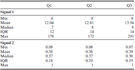
In Table 1, we present descriptive statistics for telematics data comprised in the data set, separately for each quarter. It is worth stressing that Signal 2 remains remarkably stable over the observation periods, showing that driving habits in terms of speed do not change much at aggregate level. Signal 1 appears to be more volatile as driving events are more transient. It also exhibits a moderate increasing trend within the database.
Sample statistics for raw telematics information by quarter (
 $n = 10,\,446$
). For each signal, the smallest observed value (Min), average, median, interquartile range (IQR) and largest observed value (Max) are displayed separately for the three quarters of observation (denoted, respectively, as Q1, Q2, and Q3).

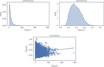
Figure 1. displays two histograms of the raw telematics data. This helps to figure out the sample distribution of the two signals entering the analysis. The scatterplot shows the correlation between them that appears to be moderately positive. In order to illustrate the treatment of a priori features, we consider here two binary covariates
 $x_1$
and
 $x_2$
(
 $p=2$
). Specifically,
 $x_1$
corresponds to the policyholder’s driving license age. It was discretized so that the value is 1 for drivers that have their driving license for more than 3 years (this represents 44% of the lines), otherwise the value is 0. The second feature
 $x_2$
corresponds to the car age. It was discretized so that the value is 1 for cars that are more than 6 year old (60% of the database), otherwise the value is 0.
Histograms for Signals 1 and 2 (upper left and right panels, respectively) and scatterplot (bottom panel) with the linear regression line.

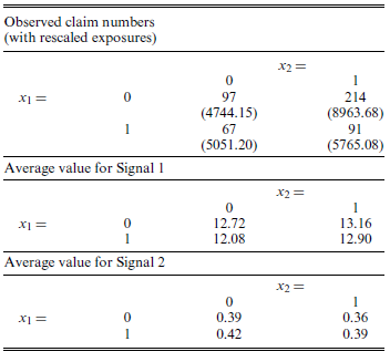
Table 2. displays the observed number of claims, together with the corresponding exposures, and the average signal values for each level of the two features. We can see there that claim frequencies and signal values are impacted by the features
 $x_1$
and
 $x_2$
so that we must enter this information in the responses to correct apparent correlation for the confounding effect of the covariates.
Observed number of claims, together with the corresponding exposures appearing within brackets, and the average signal values for each level of the binary features
 $x_1$
and
 $x_2$
.

4.3. Association between signals and claim counts
We focus specifically on the two signals presented in Section 4.1 because we expect some association between claim frequencies and numbers of dangerous driving events and speed. There is an extensive literature on how all these factors are associated to claiming. Ayuso et al. (Reference Ayuso, Guillen and Perez-Marin2016, Reference Ayuso, Guillen and Nielsen2019) showed that, among other metrics, information on speed improves the prediction of the number of claims, compared to classical models not using telematics information. Guillen et al. (Reference Guillen, Nielsen, Ayuso and Perez-Marin2019) provide an extended overview on how accumulated distance driven shows evidence that drivers improve their skills, a phenomenon that is known as the “learning effect.” All this previous knowledge is the reason why we focus specifically on variables that reflect the driving habits, such as the average speed, and for which we expect a clear association with the number of claims like the number of dangerous driving events.
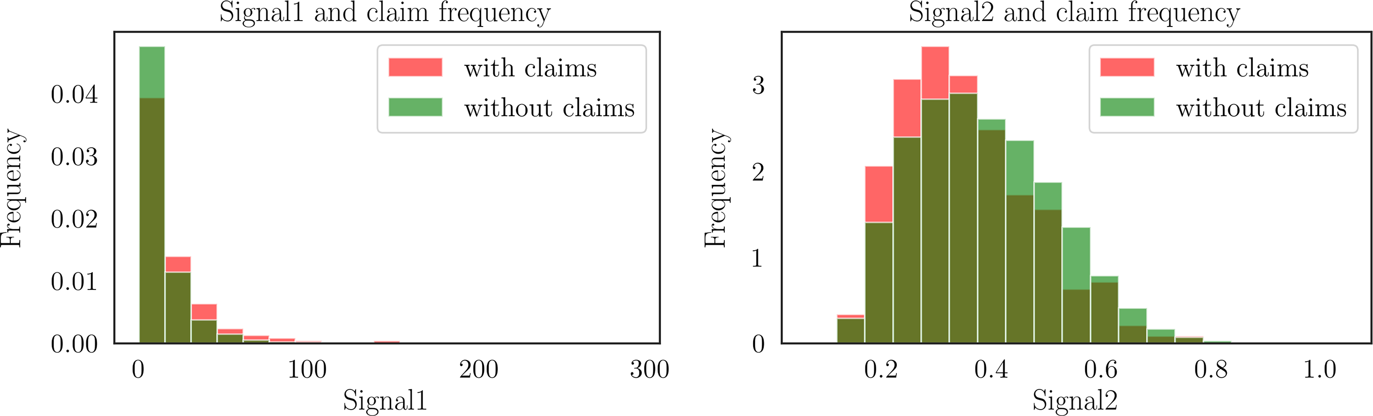
Let us now investigate the strength of this association on our data set. Figure 2 displays the frequency of claiming policyholders within each of the 20 buckets in which Signals 1 and 2 are quantized. We clearly see there that the majority of drivers having reported claims concentrate in the higher buckets for Signal 1 and in the lower buckets for Signal 2: in urban and traffic congested areas, where the average speed is lower than rural and peri-urban areas, the crash risk is higher. Thus, the association between signals and claim frequencies seems to be present in the data set under consideration.
Signals 1 and 2 and claim frequency.

We also assess the strength of nonlinear dependence between the signals and the claim counts with the help of the Hirschfeld–Gebelein–Renyi (HGR) maximal correlation coefficient proposed by Grari et al. (Reference Grari, Lamprier and Detyniecki2020). The HGR coefficient is equal to 0 if the two random variables are independent. If they are perfectly dependent, the value is 1. Note that although the claim counts is integer-valued, the HGR still captures nonlinear dependence since it corresponds to Chi-square divergence in this specific case. We obtain an estimated HGR coefficient of
 $0.048$
between claim count and Signal 1. For Signal 2, the estimation is
 $0.030$
. Signal 1 seems therefore to capture more information about the claim counts than Signal 2. Notice that the nonlinear dependence between Signals 1 and 2 is 0.200.
4.4. Fitted models
We have to estimate the scores
 $\eta$
for claim numbers and
 $\nu_k$
,
 $k=1,2$
, for Signals 1 and 2, including the two features
 $x_1$
and
 $x_2$
, as well as dispersion parameters
 $\sigma_\Delta^2$
for claim numbers,
 $\sigma_{\Gamma,1}^2$
for Signal 1, and
 $\phi_2$
and
 $\sigma_{\Gamma,2}^2$
for Signal 2. These are the marginal parameters involved in the distribution of the number of claims and of the two signals included in the analysis. Then, the off-diagonal elements of the variance–covariance matrix
 $\boldsymbol{\Sigma}$
joining the random effects in claim counts and in the available signals must also be estimated, to allow for information transfer from signal to claim frequencies.
 $S_{i,1,t}$
is modeled using a Poisson regression with its natural link function while
 $S_{i,2,t}$
is modeled using a Gamma regression using the logarithm link function.
Marginal parameters are generally well estimated by regression models fitted separately to claim frequencies and signal values. This is why the stopping criterion generally concentrates on the variance–covariance matrix
 $\boldsymbol{\Sigma}$
joining the claim counts to the available signals. Several distances are available to assess the proximity of two matrices. Some of them have been designed specifically for variance–covariance matrices, such as Bhattacharyya and Kullback-Leibler distance between two Gaussian distributions having the same location vector. In this paper, we use the following simple rule: we decide to stop the ECM algorithm as soon as the maximum relative difference between correlation coefficients
 $\rho_{\Delta,\Gamma,k}$
at two successive steps become smaller than a predefined tolerance level.
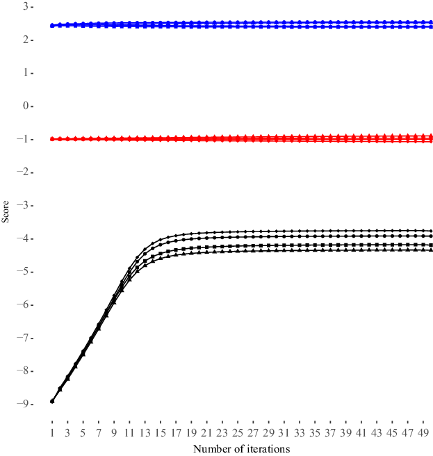
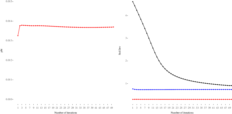
Figures 3 and 4 display the estimations with respect to the number of iterations. After about 50 iterations, the estimations stabilize and the stopping criterion is fulfilled. We end up with the following estimates for the scores
 \begin{eqnarray*}\widehat{\eta}(\boldsymbol{x})&=& -3.912 -0.423 x_1 + 0.155 x_2 \\\widehat{\nu}_1(\boldsymbol{x})&=&2.557 -0.025 x_1 -0.134 x_2 \\\widehat{\nu}_2(\boldsymbol{x})&=&-0.989 + 0.103 x_1 -0.073 x_2\end{eqnarray*}
involved in the number of claims
 $N_{it}$
, Signal 1, and Signal 2, respectively. The variance–covariance matrix of the multivariate Normal distribution for the random vector
 $(\Delta,\Gamma_1,\Gamma_2)$
is estimated to
 \begin{equation*} \widehat{\boldsymbol{\Sigma}}=\begin{pmatrix}0.835608624 &0.01087129&-0.003205314 \\0.010871290 &0.54745657 &0.020714447 \\-0.003205314 &0.02071445 &0.092999400\end{pmatrix}.\end{equation*}
In accordance with the exploratory analysis, we get a negative correlation between
 $\Delta$
and
 $\Gamma_2$
and a positive correlation between
 $\Delta$
and
 $\Gamma_1$
. Despite the relatively small estimated correlations, signals induce strong a posteriori corrections, as shown next (recall from Section 2 that correlations between responses involve the exponential transform of the elements in
 $\widehat{\boldsymbol{\Sigma}}$
).
Scores estimates
 $\widehat{\eta}(\boldsymbol{x})$
(in black),
 $\widehat{\nu}_1(\boldsymbol{x})$
(in blue), and
 $\widehat{\nu}_2(\boldsymbol{x})$
(in red) along algorithm iterations for
 $\boldsymbol{x}=(0,0)$
(circle),
 $\boldsymbol{x}=(1,0)$
(triangle),
 $\boldsymbol{x}=(0,1)$
(diamond), and
 $\boldsymbol{x}=(1,1)$
(square).

Estimation of the dispersion parameter
 $\phi_2$
along algorithm iterations (left). Estimations of the standard deviations
 $\sigma_\Delta$
(in black),
 $\sigma_{\Gamma,1}$
(in blue), and
 $\sigma_{\Gamma,2}$
(in red) along algorithm iterations (right).

Eventually, to benchmark our final fitted model, two other models were trained. The simplest trained model consists in assigning to every row the average claim frequency. Then a model was trained using only the two traditional variables. The Poisson deviance of different models is showed in Table 3. The final model shows an important improvement compared to the simple models.
Models deviance

4.5. Credibility updating formulas
In the classical actuarial approach based on claim counts, only, past numbers of claims enter the credibility formulas in addition to observable features
 $\boldsymbol{x}_{i,T_i+1}$
to explain
 $N_{i,T_i+1}$
. Formally, the experience used to revise future premiums relates to past claims history, only, and is henceforth denoted as
 \begin{equation*}\mathcal{H}_{i,T_i}^{\text{claim}}=\{N_{i,t},t=1,\ldots,T_i\}.\end{equation*}
This information enters the predictive distribution, i.e. the conditional distribution of
 $N_{i,T_i+1}$
given
 $\mathcal{H}_{i,T_i}^{\text{claim}}$
. With experience rating, the a priori expectation
 \begin{equation*}\text{E}[N_{i,T_i+1}]=\lambda_{i,T_i+1}\text{E}[\exp(\Delta_i)]\end{equation*}
is replaced with the a posteriori expectation
 \begin{equation*}\text{E}[N_{i,T_i+1}|\mathcal{H}_{i,T_i}^{\text{claim}}]=\lambda_{i,T_i+1}\text{E}[\exp(\Delta_i)|\mathcal{H}_{i,T_i}^{\text{claim}}].\end{equation*}
The pricing structure is slow to adapt in personal lines because the expected claim frequencies are generally small, whatever the driver’s risk profile.
The approach proposed in this paper recognizes the a posteriori nature of telematics data. The multivariate credibility model developed in the present case study captures the association between Signals 1-2 and claim counts, allowing the actuary to refine risk evaluations based on past history. With telematics, past claims history
 $\mathcal{H}_{i,T_i}^{\text{claim}}$
is enriched with behavioral data. This allows the pricing structure to become more reactive. In this case, the policy-specific history
 $\mathcal{H}_{i,T_i}$
gathers all the a posteriori information
 \begin{equation*}\mathcal{H}_{i,T_i}=\mathcal{H}_{i,T_i}^{\text{claim}}\cup\mathcal{H}_{i,T_i}^{\text{signals}}=\{(N_{i,t},S_{i,1,t},S_{i,2,t}),t=1,\ldots,T_i\}.\end{equation*}
The multivariate mixed/credibility model describes the joint dynamics of
 $(N_{i,t}, S_{i,1,t},S_{i,2,t})$
, given a priori features
 $\boldsymbol{x}_{i,t}$
. The predictive distribution now corresponds to the conditional distribution of
 $N_{i,T_i+1}$
given
 $\mathcal{H}_{i,T_i}$
. The a priori expectation is replaced with an a posteriori one
 \begin{equation*}\text{E}[N_{i,T_i+1}|\mathcal{H}_{i,T_i}]=\lambda_{i,T_i+1}\text{E}[\exp(\Delta_i)|\mathcal{H}_{i,T_i}],\end{equation*}
so that the factor
 $\text{E}[\exp(\Delta_i)|\mathcal{H}_{i,T_i}]/\text{E}[\exp(\Delta_i)|\mathcal{H}_{i,T_i}^{\text{claim}}]$
corresponds to the improvement we get for the a posteriori correction by also using the behavioral data provided by telematics.
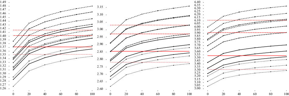
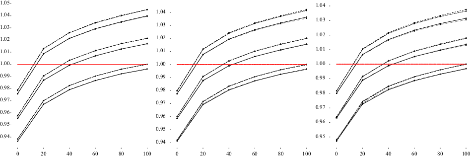
Figures 5 and 6 depict the a posteriori corrections
 $\text{E}[\exp(\Delta_i)|\mathcal{H}_{i,T_i}]$
and
 $\text{E}[\exp(\Delta_i)|\mathcal{H}_{i,T_i}^{\text{claim}}]$
together with the factor
 $\text{E}[\exp(\Delta_i)|\mathcal{H}_{i,T_i}]/\text{E}[\exp(\Delta_i)|\mathcal{H}_{i,T_i}^{\text{claim}}]$
for
 $\boldsymbol{x}=(0,0)$
,
 $\boldsymbol{x}=(1,0)$
,
 $\boldsymbol{x}=(0,1)$
and
 $\boldsymbol{x}=(1,1)$
. Horizontal lines correspond to a posteriori corrections based on
 $\mathcal{H}_{i,T_i}^{\text{claim}}$
, whereas trending curves illustrate the impact of incorporating past signal values in premium corrections.
Left:
 $N_{i,1}+N_{i,2}+N_{i,3}=0$
, Middle:
 $N_{i,1}+N_{i,2}+N_{i,3}=1$
, Right:
 $N_{i,1}+N_{i,2}+N_{i,3}=2$
.
 $\text{E}[\exp(\Delta_i)|\mathcal{H}_{i,T_i}]$
(in black) and
 $\text{E}[\exp(\Delta_i)|\mathcal{H}_{i,T_i}^{\text{claim}}]$
(in red) for
 $(S_{i,2,1}=0.20,S_{i,2,2}=0.20,S_{i,2,3}=0.20)$
(circles),
 $(S_{i,2,1}=0.40,S_{i,2,2}=0.40,S_{i,2,3}=0.40)$
(triangles),
 $(S_{i,2,1}=0.70,S_{i,2,2}=0.70,S_{i,2,3}=0.70)$
(diamonds) and
 $S_{i,1,1}+S_{i,1,2}+S_{i,1,3}=0,20,40,60,80,100$
.
 $\boldsymbol{x}=(0,0)$
(solid line),
 $\boldsymbol{x}=(1,0)$
(dashed line),
 $\boldsymbol{x}=(0,1)$
(dotted line),
 $\boldsymbol{x}=(1,1)$
(two dash line).

Left:
 $N_{i,1}+N_{i,2}+N_{i,3}=0$
, Middle:
 $N_{i,1}+N_{i,2}+N_{i,3}=1$
, Right:
 $N_{i,1}+N_{i,2}+N_{i,3}=2$
.
 $\text{E}[\exp(\Delta_i)|\mathcal{H}_{i,T_i}]/\text{E}[\exp(\Delta_i)|\mathcal{H}_{i,T_i}^{\text{claim}}]$
for
 $(S_{i,2,1}=0.20,S_{i,2,2}=0.20,S_{i,2,3}=0.20)$
(circles),
 $(S_{i,2,1}=0.40,$
 $S_{i,2,2}=0.40,S_{i,2,3}=0.40)$
(triangles),
 $(S_{i,2,1}=0.70,S_{i,2,2}=0.70,S_{i,2,3}=0.70)$
(diamonds) and
 $S_{i,1,1}+S_{i,1,2}+S_{i,1,3}=0,20,40,60,80,100$
.
 $\boldsymbol{x}=(0,0)$
(solid line),
 $\boldsymbol{x}=(1,0)$
(dashed line),
 $\boldsymbol{x}=(0,1)$
(dotted line),
 $\boldsymbol{x}=(1,1)$
(two dash line).

For each value of
 $\boldsymbol{x}$
, one sees that both a posteriori corrections
 $\text{E}[\exp(\Delta_i)|\mathcal{H}_{i,T_i}]$
and
 $\text{E}[\exp(\Delta_i)|\mathcal{H}_{i,T_i}^{\text{claim}}]$
increase with the total number of claims
 $N_{i,1}+N_{i,2}+N_{i,3}$
observed over the last three periods. Furthermore,
 $\text{E}[\exp(\Delta_i)|\mathcal{H}_{i,T_i}]$
also increases with the total number of dangerous driving events
 $S_{i,1,1}+S_{i,1,2}+S_{i,1,3}$
observed over the last three periods while it decreases with the normalized average speeds
 $(S_{i,2,1},S_{i,2,2},S_{i,2,3})$
. For instance, a policyholder belonging to the reference risk class
 $\boldsymbol{x}=(0,0)$
who made no claim over the last three periods (here the last 9 months) and recording 10 dangerous driving events in total can see its expected claim frequency decreases by approximately 5% by using telematics data (i.e.
 $\text{E}[\exp(\Delta_i)|\mathcal{H}_{i,T_i}]/\text{E}[\exp(\Delta_i)|\mathcal{H}_{i,T_i}^{\text{claim}}] \approx 95\%$
) when its normalized average speeds are equal to
 $0.7$
over the last three periods.
Finally, one can notice that the factor
 $\text{E}[\exp(\Delta_i)|\mathcal{H}_{i,T_i}]/\text{E}[\exp(\Delta_i)|\mathcal{H}_{i,T_i}^{\text{claim}}]$
is stable from one risk class to another. As expected, when comparing two drivers in two different risk classes, the one with the lower a priori claim frequency has higher a posteriori corrections
 $\text{E}[\exp(\Delta_i)|\mathcal{H}_{i,T_i}]$
and
 $\text{E}[\exp(\Delta_i)|\mathcal{H}_{i,T_i}^{\text{claim}}]$
.
Figures 5 and 6 show that despite relatively low estimated correlations, past signal values induce further segmentation among insured drivers, beyond that resulting from the inclusion of
 $\mathcal{H}_{i,T_i}^{\text{claim}}$
in premium calculation. This is particularly encouraging for practical applications since with only two signals that can easily be communicated to policyholders, the credibility model is able to capture quite a large part of residual heterogeneity after just three periods when supplementing
 $\mathcal{H}_{i,T_i}^{\text{claim}}$
with
 $\mathcal{H}_{i,T_i}^{\text{signals}}$
.
4.6. Algorithm extensibility
We illustrate how the ECM algorithm can accept other signals extending the previous use case adding a third signal that is
 \begin{eqnarray*}S_{i,3,t} &=& \text{distance driven for Policyholder {i} in period {t}}.\end{eqnarray*}
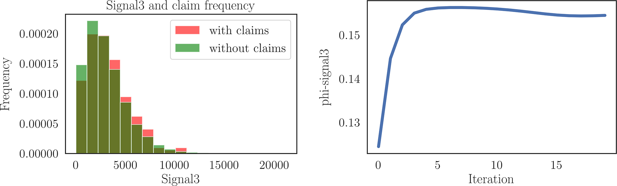
In Figure 7, we show the new signal distribution, differentiated by the presence of claims. We use a Gamma distribution to model
 $S_{i,3,t}$
and Figure 7 also displays
 $\widehat{\phi}_3$
already converging after 20 iterations. The new random effect
 $\Gamma_3$
is negatively correlated with
 $\Delta$
, namely
 $\widehat{\text{Cov}}[\Delta,\Gamma_3]=-0.030606301$
, which can be explained by the superposition of the learning effect (one gains experience while driving, as documented, e.g. in Boucher et al., Reference Boucher, Perez-Marin and Santolino2013) and a driving environment effect: those who drive very long distances do so on highways, thus generally outside residential areas. Figure 8 displays the factor
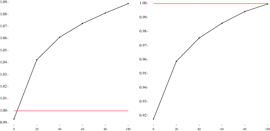
 $\text{E}[\exp(\Delta_i)|\mathcal{H}_{i,T_i}]/\text{E}[\exp(\Delta_i)|\mathcal{H}_{i,T_i}^{\text{claim}}]$
for a policyholder i of the reference class (
 $\boldsymbol{x}_i=(0,0)$
) who made no claims over the last three periods (
 $N_{i,1}+N_{i,2}+N_{i,3}=0$
) and with average values for Signal 2
 $(S_{i,2,1}=0.40,S_{i,2,2}=0.40,S_{i,2,3}=0.40)$
. Compared to the left of Figure 6 (solid line with triangles), one sees that low (resp. high) values for Signal 3, here
 $(S_{i,3,1}=500,S_{i,3,2}=500,S_{i,3,3}=500)$
(resp.
 $(S_{i,3,1}=5000,S_{i,3,2}=5000,S_{i,3,3}=5000)$
), yield higher (resp. lower) premium corrections.
Signals 3 distribution, claim frequency, and convergence.

 $\text{E}[\exp(\Delta_i)|\mathcal{H}_{i,T_i}]/\text{E}[\exp(\Delta_i)|\mathcal{H}_{i,T_i}^{\text{claim}}]$
for
 $\boldsymbol{x}_i=(0,0)$
,
 $N_{i,1}+N_{i,2}+N_{i,3}=0$
,
 $(S_{i,2,1}=0.40,S_{i,2,2}=0.40,S_{i,2,3}=0.40)$
and
 $S_{i,1,1}+S_{i,1,2}+S_{i,1,3}=0,20,40,60,80,100$
. Left:
 $(S_{i,3,1}=500,S_{i,3,2}=500,S_{i,3,3}=500)$
, Right:
 $(S_{i,3,1}=5000,S_{i,3,2}=5000,S_{i,3,3}=5000)$
.

5. Conclusion
Pay-How-You-Drive (PHYD) motor insurance complements traditional actuarial models with data reflecting driving behavior (e.g., vehicle average speed) and external risk factors (e.g., time of the day). Such data are recorded and transmitted by telematics devices embedded in each vehicle.
In this paper, we exploit the a posteriori nature of telematics data and their heterogeneity among insured drivers. We study a multivariate mixed model that extends the model describing the joint dynamics of telematics data and claim frequencies proposed by Denuit et al. (Reference Denuit, Guillen and Trufin2019a) by replacing the estimation procedure with the ECM algorithm. The proposed model enables to combine telematics signals with various formats and claim counts, refining risk evaluations based on drivers’ recent history.
Numerical illustrations carried on a real, but simplified data set with two and three telematics signals of different formats suggest that the proposed approach is already able to capture quite a large part of residual heterogeneity after just few months monitoring, allowing the pricing structure to become more reactive.
Appendix A Evaluation of the conditional expectations involved in the ECM algorithm
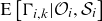
The ECM approach involves conditional expectations of the random effects in each E-step. Here, we carefully explain how to compute
 $\text{E}\left[ \Delta_i | \mathcal{O}_i, \mathcal{S}_i \right]$
and
 $\text{E}\left[ \Gamma_{i,k} | \mathcal{O}_i, \mathcal{S}_i \right]$
so that the reader can easily adapt the formulas to the other conditional expectations appearing in the ECM algorithm.
We have
 \begin{eqnarray*}\text{E}\left[ \Delta_i | \mathcal{O}_i, \mathcal{S}_i \right] =\int_{-\infty}^\infty \delta f_{\Delta_i|\mathcal{O}_i, \mathcal{S}_i}(\delta) \mathrm{d}\delta\end{eqnarray*}
where
 $f_{\Delta_i|\mathcal{O}_i, \mathcal{S}_i}$
denotes the conditional probability density function of
 $\Delta_i$
given past observations
 $\mathcal{O}_i$
and past values of the scores
 $\mathcal{S}_i$
. Assume that the signals
 $S_{i,k,t}$
are continuous, with conditional probability density function
 $f_{S_{i,k,t}|\Gamma_{i,k}=\gamma_k}(\cdot)$
given
 $\Gamma_{i,k}=\gamma_k$
. For discrete signals, the conditional probability density function is replaced with the conditional probability mass function. The conditional expectation can then be expressed as the ratio
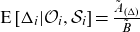 $\text{E}\left[ \Delta_i | \mathcal{O}_i, \mathcal{S}_i \right] = \frac{\tilde{A}_{(\Delta)}}{\tilde{B}}$
with
 \begin{eqnarray*}\tilde{A}_{(\Delta)}&=& \int_{-\infty}^\infty \ldots \int_{-\infty}^\infty \delta\prod_{t=1}^{T_i}\left(\text{P}[N_{i,t}=n_{i,t}|\Delta_i=\delta]\prod_{k=1}^q f_{S_{i,k,t}|\Gamma_{i,k}=\gamma_k}(s_{i,k,t}) \right) \\&& f_{\boldsymbol{\Sigma}}(\delta,\gamma_{1},\ldots,\gamma_{q}) \mathrm{d}\delta \mathrm{d}\gamma_1 \ldots \mathrm{d}\gamma_q\end{eqnarray*}
and
 \begin{eqnarray*}\tilde{B}&=& \int_{-\infty}^\infty \ldots \int_{-\infty}^\infty \prod_{t=1}^{T_i}\left(\text{P}[N_{i,t}=n_{i,t}|\Delta_i=\delta]\prod_{k=1}^q f_{S_{i,k,t}|\Gamma_{i,k}=\gamma_k}(s_{i,k,t}) \right) \\&& f_{\boldsymbol{\Sigma}}(\delta,\gamma_{1},\ldots,\gamma_{q}) \mathrm{d}\delta \mathrm{d}\gamma_1 \ldots \mathrm{d}\gamma_q.\end{eqnarray*}
Under the assumptions of our model, we know that given
 $\Delta_i=\delta$
,
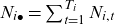 $N_{i\bullet}=\sum_{t=1}^{T_i}N_{i,t}$
obeys the Poisson
 $\big(\lambda_{i\bullet}\exp(\delta)\big)$
distribution where
 $\lambda_{i\bullet}=\sum_{t=1}^{T_i}d_{i,t}\exp(\eta_{i,t})$
. Therefore,
 $\text{E}\left[ \Delta_i | \mathcal{O}_i, \mathcal{S}_i \right]=\frac{\tilde{A}_{(\Delta)}}{\tilde{B}}=\frac{A_{(\Delta)}}{B}$
with
 \begin{eqnarray*}A_{(\Delta)}&=& \int_{-\infty}^\infty \ldots \int_{-\infty}^\infty \delta (\exp(\delta))^{n_{i\bullet}} \exp(-\lambda_{i\bullet} \exp(\delta))\prod_{t=1}^{T_i}\prod_{k=1}^q f_{S_{i,k,t}|\Gamma_{i,k}=\gamma_k}(s_{i,k,t}) \\&& f_{\boldsymbol{\Sigma}}(\delta,\gamma_{1},\ldots,\gamma_{q}) \mathrm{d}\delta \mathrm{d}\gamma_1 \ldots \mathrm{d}\gamma_q\end{eqnarray*}
and
 \begin{eqnarray*}B&=& \int_{-\infty}^\infty \ldots \int_{-\infty}^\infty (\exp(\delta))^{n_{i\bullet}} \exp(-\lambda_{i\bullet} \exp(\delta))\prod_{t=1}^{T_i}\prod_{k=1}^q f_{S_{i,k,t}|\Gamma_{i,k}=\gamma_k}(s_{i,k,t}) \\&& f_{\boldsymbol{\Sigma}}(\delta,\gamma_{1},\ldots,\gamma_{q}) \mathrm{d}\delta \mathrm{d}\gamma_1 \ldots \mathrm{d}\gamma_q\end{eqnarray*}
where
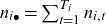 $n_{i\bullet}=\sum_{t=1}^{T_i}n_{i,t}$
stands for the observed claim totals
 $N_{i\bullet}$
.
Similarly, we can write
 $\text{E}\left[ \Gamma_{i,k_0} | \mathcal{O}_i, \mathcal{S}_i \right]=\frac{A_{(\Gamma_{k_0})}}{B}$
for each signal
 $\Gamma_{i,k_0}$
with
 \begin{eqnarray*}A_{(\Gamma_{k_0})}&=& \int_{-\infty}^\infty \ldots \int_{-\infty}^\infty \gamma_{k_0}(\exp(\delta))^{n_{i\bullet}} \exp(-\lambda_{i\bullet} \exp(\delta))\prod_{t=1}^{T_i}\prod_{k=1}^q f_{S_{i,k,t}|\Gamma_{i,k}=\gamma_k}(s_{i,k,t}) \\&& f_{\boldsymbol{\Sigma}}(\delta,\gamma_{1},\ldots,\gamma_{q}) \mathrm{d}\delta \mathrm{d}\gamma_1 \ldots \mathrm{d}\gamma_q\end{eqnarray*}
and
 \begin{eqnarray*}B&=& \int_{-\infty}^\infty \ldots \int_{-\infty}^\infty (\exp(\delta))^{n_{i\bullet}} \exp(-\lambda_{i\bullet} \exp(\delta))\prod_{t=1}^{T_i}\prod_{k=1}^q f_{S_{i,k,t}|\Gamma_{i,k}=\gamma_k}(s_{i,k,t}) \\&& f_{\boldsymbol{\Sigma}}(\delta,\gamma_{1},\ldots,\gamma_{q}) \mathrm{d}\delta \mathrm{d}\gamma_1 \ldots \mathrm{d}\gamma_q.\end{eqnarray*}
Conditional expectations appearing at iteration
 $l=0,1,2,\ldots$
of the ECM algorithm (iteration
 $l=0$
corresponding to the initialization) are then obtained by replacing
 $\mathcal{S}_i $
with
 $\mathcal{S}_i ^{(l)}$
. The integrals involved in these formulas can be computed using quadratures, as explained in Pechon et al. (Reference Pechon, Trufin and Denuit2018, Reference Pechon, Denuit and Trufin2019, Reference Pechon, Denuit and Trufin2021). Gauss–Hermite quadratures revealed itself to be fast, especially when used in conjunction with the package Rcpp which allows to write chunk of codes in C++ inside an R script enabling a drastic reduction in computational time (up to 30 times faster).