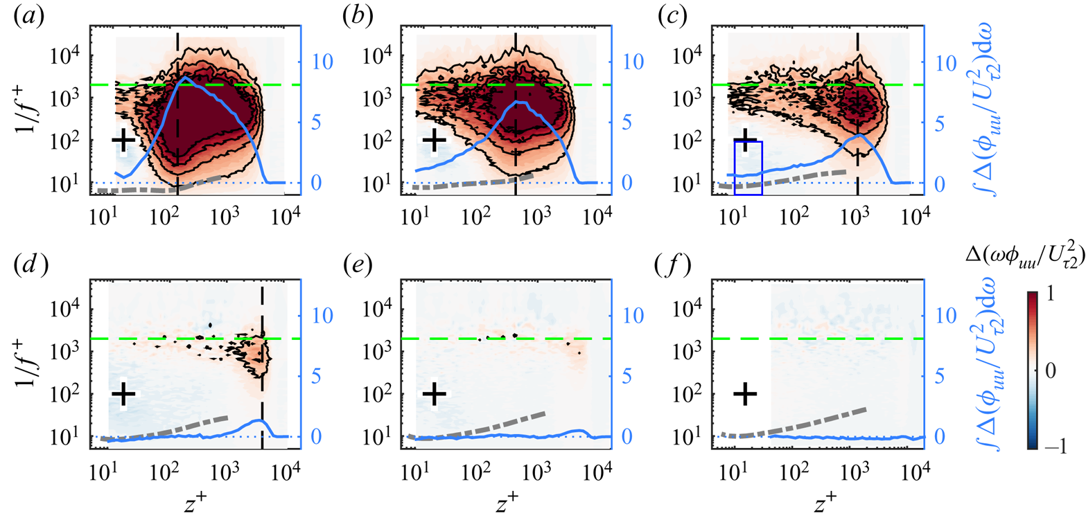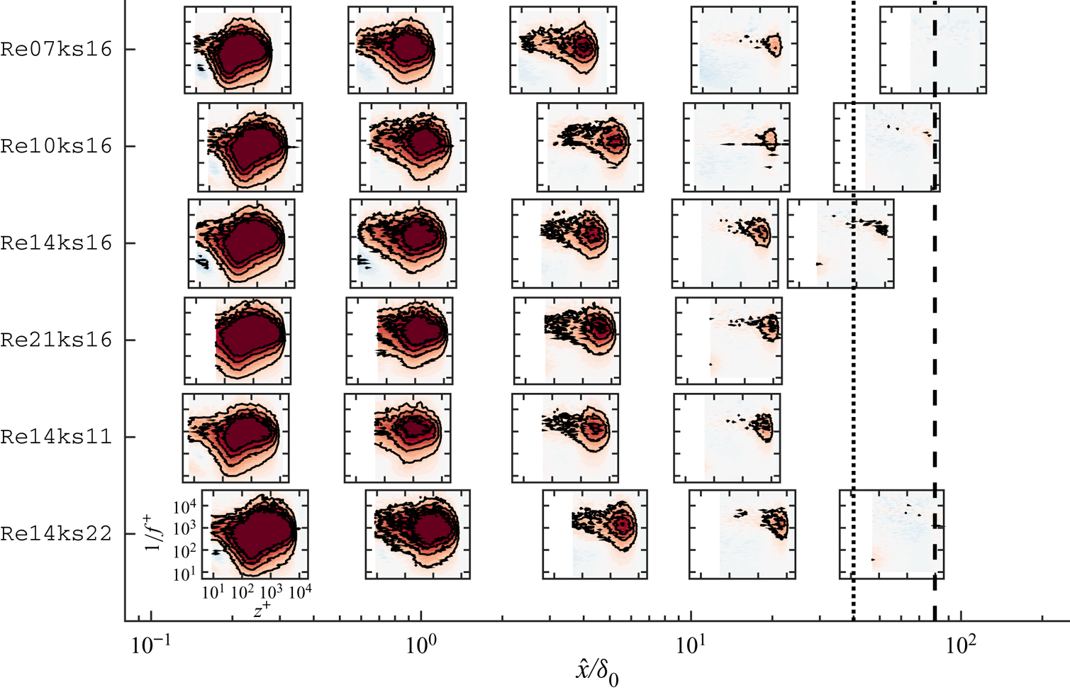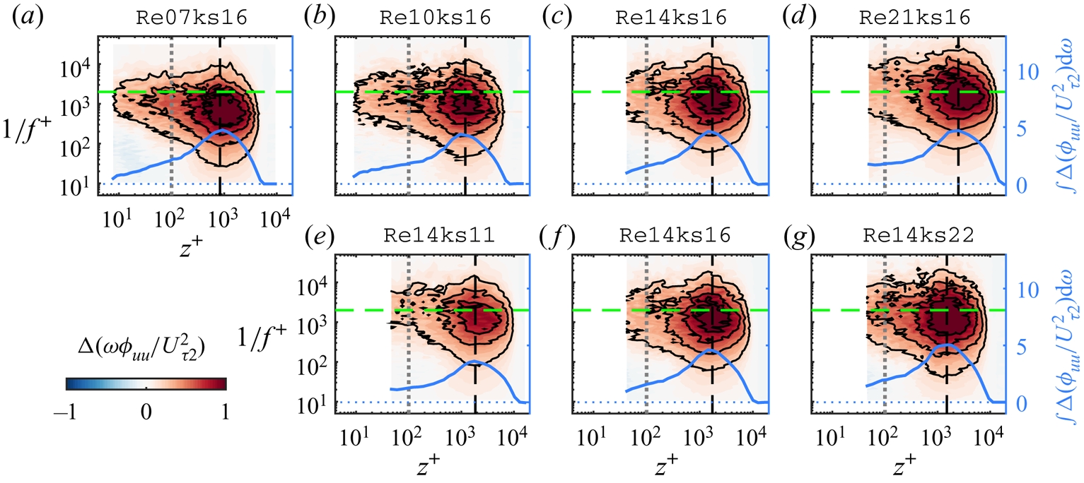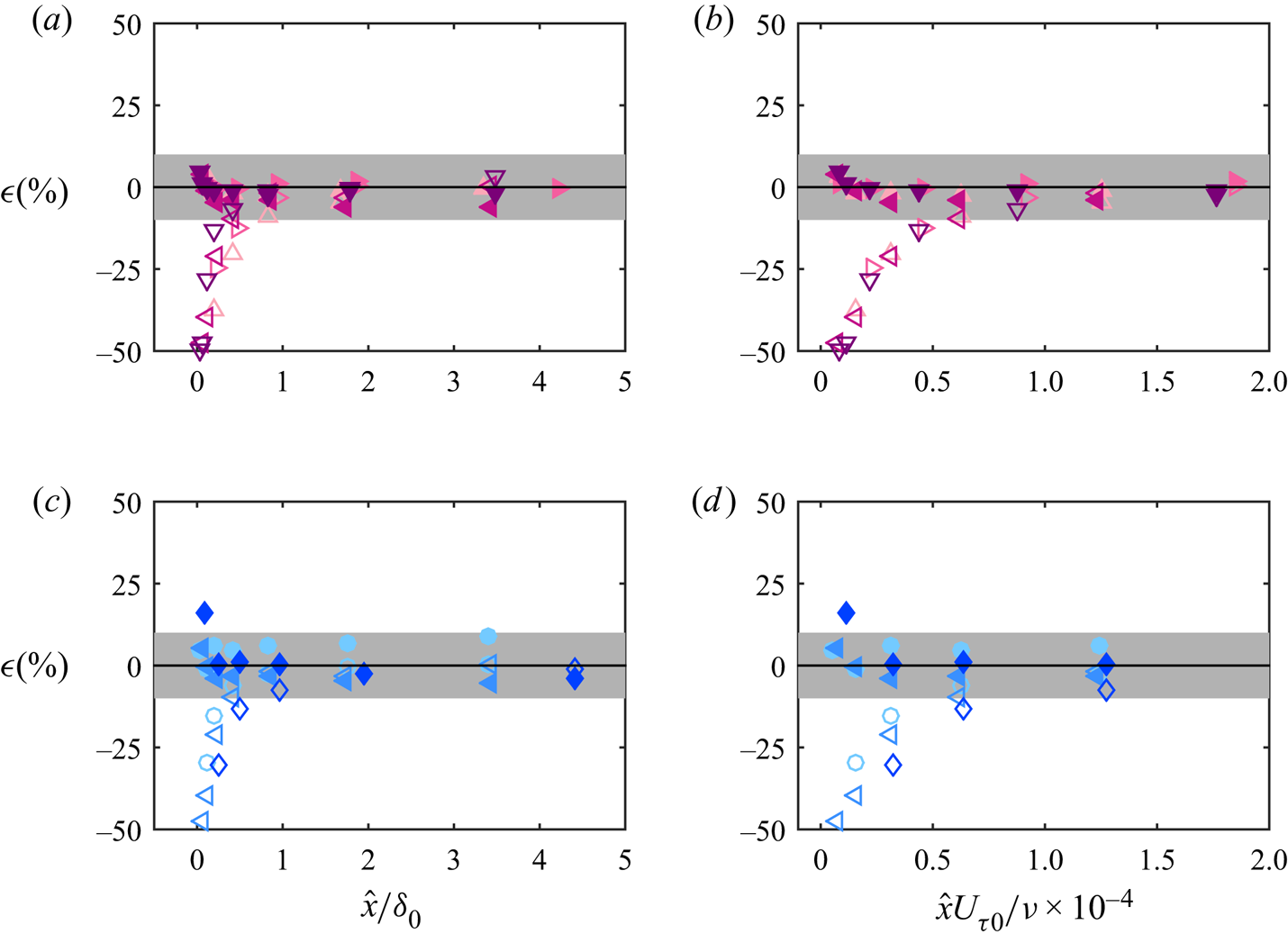



1. Introduction
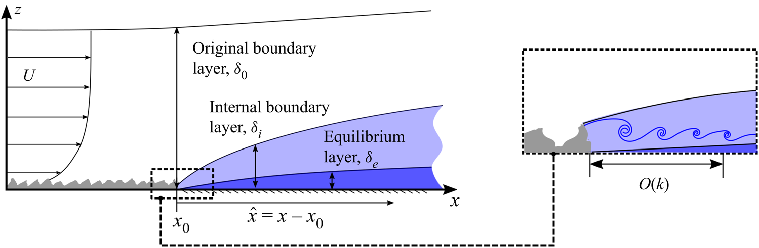
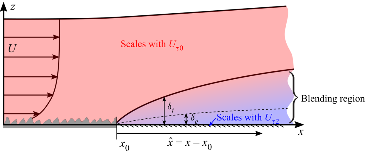
Surface roughness with heterogeneity is present in wall-bounded turbulent flows in a variety of conditions. Examples include the patchiness of biofouling on the hull of a ship or the changes in the surface roughness conditions that occur at the interface between forest and grasslands. Understanding the flow response to such a change in the surface condition is beneficial to various practical applications such as predicting the drag penalty introduced by non-uniform fouling or improving the weather forecast in regions with a change of terrain. Although roughness heterogeneity can occur in a number of configurations, here we consider a simple scenario, namely a sudden rough-to-smooth surface transition occurring in the streamwise direction, as depicted in figure 1. Upstream of the transition, a turbulent boundary layer develops on a rough wall with equivalent sand grain roughness height  $k_s$. Here,
 $x$ is the streamwise direction,
 $x_0$ is the streamwise location of the surface transition and
 $\hat {x} \equiv x - x_0$ is the distance downstream of the transition. At
 $x=x_0$, the surface switches to a smooth wall, while the boundary layer continues to evolve and gradually adjusts to the new surface. The effect of the new surface condition is first felt in the near-wall region of the boundary layer and then gradually propagates to the interior of the flow (Garratt Reference Garratt1990). The layer that separates the modified near-wall region from the unaffected oncoming flow further away from the wall is generally referred to as the internal boundary layer (IBL) with a thickness denoted by
 $\delta _i$. The complete adjustment of flow statistics to the downstream wall condition (referred to here as equilibrium) also first emerges in the region immediately adjacent to the smooth wall. This region is referred to as the equilibrium layer (EL) (Garratt Reference Garratt1990; Savelyev & Taylor Reference Savelyev and Taylor2005) with thickness
 $\delta _e$. In most cases, a large portion of the flow within the IBL has still not fully adapted to the local wall condition (Antonia & Luxton Reference Antonia and Luxton1972; Ismail, Zaki & Durbin Reference Ismail, Zaki and Durbin2018; Li et al. Reference Li, de Silva, Baidya, Rouhi, Chung, Marusic and Hutchins2019; Rouhi, Chung & Hutchins Reference Rouhi, Chung and Hutchins2019a), and a general consensus is that
 $\delta _e\approx 0.05\delta _i$, where
 $\delta _i$ is defined based on the shear stress profile adjustment downstream of a rough-to-smooth change (see Shir Reference Shir1972; Rao, Wyngaard & Coté Reference Rao, Wyngaard and Coté1974). The term ‘transition layer’ is sometimes used for the region between the EL and IBL (Savelyev & Taylor Reference Savelyev and Taylor2005). As shown in the inset of figure 1, immediately downstream of the rough-to-smooth change, a region exists where we would expect a recirculation region to form, as a result of the step in the surface elevation between the rough and smooth walls which produces vortex shedding from the roughness crests. Similar to backward facing steps (Kostas, Soria & Chong Reference Kostas, Soria and Chong2002; Barri et al. Reference Barri, El Khoury, Andersson and Pettersen2010; Wu, Ren & Tang Reference Wu, Ren and Tang2013; Rouhi, Chung & Hutchins Reference Rouhi, Chung and Hutchins2019b), this region (which we refer to as the ‘roughness trailing wake’) persists over a streamwise fetch that scales on the roughness height, before the intensity attenuates and falls below the local turbulence intensity of the existing turbulent boundary layer.
Schematic of a turbulent boundary layer over a rough-to-smooth change in surface condition. The roughness transition occurs at  $x_0$, and
 $\hat {x} = x-x_0$ denotes the fetch downstream of the transition. The inset is a zoom-in view of the boxed region close to the rough-to-smooth change, where a trail of vortices are shed from the roughness elements.

The study on flows over a streamwise roughness transition started in the meteorology community driven by the need to understand the effect of a change in the terrain on the microclimate (Elliott Reference Elliott1958; Bradley Reference Bradley1968; Shir Reference Shir1972; Rao et al. Reference Rao, Wyngaard and Coté1974). These studies focused on deep surface layers with the upstream and downstream surfaces assumed to be fully rough. Such flows are dependent on a single parameter, the magnitude of roughness change (usually denoted by  $M$ and defined as a function of the ratio between the upstream and downstream roughness lengths). Further studies on turbulent boundary layers with a finite thickness (mainly experimental, see Antonia & Luxton Reference Antonia and Luxton1972; Hanson & Ganapathisubramani Reference Hanson and Ganapathisubramani2016; Li et al. Reference Li, de Silva, Baidya, Rouhi, Chung, Marusic and Hutchins2019, for example) and channel flows (mainly numerical, see Bou-Zeid, Meneveau & Parlange Reference Bou-Zeid, Meneveau and Parlange2004; Saito & Pullin Reference Saito and Pullin2014; Ismail et al. Reference Ismail, Zaki and Durbin2018; Rouhi et al. Reference Rouhi, Chung and Hutchins2019a, for example) have appeared in recent years. In either case, a new length scale of the outer flow (the boundary layer thickness or the channel half height) becomes more relevant, and the flow response is expected to be dependent on both the magnitude of roughness change and a new non-dimensional parameter involving the outer length scale. This will be especially meaningful further away from the roughness transition where the IBL is comparable with the local boundary layer thickness.
Downstream of the rough-to-smooth transition, the skin-friction coefficient undershoots the corresponding smooth-wall value before gradually recovering in the far-field (Antonia & Luxton Reference Antonia and Luxton1972; Hanson & Ganapathisubramani Reference Hanson and Ganapathisubramani2016; Ismail et al. Reference Ismail, Zaki and Durbin2018; Li et al. Reference Li, de Silva, Baidya, Rouhi, Chung, Marusic and Hutchins2019; Rouhi et al. Reference Rouhi, Chung and Hutchins2019a). The deviation of the mean flow within the IBL from a self-similar canonical smooth-wall boundary layer leads to an underestimation of the skin-friction coefficient in both ‘indirect’ measurements (Loureiro et al. Reference Loureiro, Sousa, Zotin and Freire2010; Li et al. Reference Li, de Silva, Baidya, Rouhi, Chung, Marusic and Hutchins2019), such as the Clauser chart method or Preston tube (Patel Reference Patel1965), and the predictive model of Elliott (Reference Elliott1958), where an equilibrium log-law profile is assumed within the IBL. There have been various attempts to model the adjusting flow within the IBL, either by using a local shear stress that varies in the wall-normal direction in a mixing-length model (Panofsky & Townsend Reference Panofsky and Townsend1964; Ghaisas Reference Ghaisas2020), or by linearly blending the corresponding upstream and downstream mean velocity profiles (Chamorro & Porté-Agel Reference Chamorro and Porté-Agel2009). The non-equilibrium behaviour of the adjusting flow also manifests in turbulence statistics, such as the higher magnitude of Reynolds normal and shear stresses and the dissipation rate of turbulent kinetic energy (Antonia & Luxton Reference Antonia and Luxton1972; Ismail et al. Reference Ismail, Zaki and Durbin2018). For rough-to-smooth flows, the increased magnitude of the ‘inner-peak’ in the streamwise turbulence intensity profile located approximately 15 viscous units above the wall has been attributed to the superposition of energetic rough-wall structures (centred above the internal layer) onto the near-wall region (Ismail et al. Reference Ismail, Zaki and Durbin2018; Li et al. Reference Li, de Silva, Baidya, Rouhi, Chung, Marusic and Hutchins2019).
We consider a turbulent boundary layer in the fully-rough regime as the upstream flow condition prior to the roughness transition. It can be characterised by friction Reynolds number  $Re_{\tau 0}\equiv U_{\tau 0}\delta _0/\nu$ and roughness Reynolds number
 $k_{s0}^{+}\equiv U_{\tau 0}k_s/\nu$ (Jiménez Reference Jiménez2004). The subscript
 $(\cdot )_0$ denotes flow quantities on the rough wall just prior to the transition. Here,
 $U_{\tau 0}$ is the rough-wall friction velocity,
 $\delta _0$ is the boundary layer thickness at the rough-to-smooth change (boundary layer thickness
 $\delta _{99}(\hat {x})$ is defined as the wall distance where the mean streamwise velocity reaches 99 % of the free stream velocity, and
 $\delta _0\equiv \delta _{99}(0)$) and
 $\nu$ is the kinematic viscosity of air. For the rough-to-smooth change investigated here,
 $k_{s0}^{+}$ provides the magnitude of roughness change and
 $Re_{\tau 0}$ reflects the outer length scale.
Most of the existing experimental studies of a streamwise rough-to-smooth change include a small number of cases achieved by varying the free stream velocity or the morphology of the surface roughness. Both  $Re_{\tau 0}$ and
 $k_{s0}^{+}$ vary concurrently as a result, and the change of roughness morphologies may also contribute to the difference observed between cases. Although classical models, such as by Elliott (Reference Elliott1958), can capture the flow response with some success when the IBL occupies only a small fraction of the entire boundary layer, there are questions regarding the validity of such models in the far field where the friction velocity scale of the outer layer has been found to decay (Hanson & Ganapathisubramani Reference Hanson and Ganapathisubramani2016). In addition, the validity of skin-friction measurements with conventional ‘indirect’ methods, such as the Clauser chart method or Preston tube (Patel Reference Patel1965), is compromised within a few boundary layer thicknesses downstream of the roughness transition, where such methods rely on erroneous assumptions of canonical smooth-wall behaviours beyond the EL (Loureiro et al. Reference Loureiro, Sousa, Zotin and Freire2010; Li et al. Reference Li, de Silva, Baidya, Rouhi, Chung, Marusic and Hutchins2019). Furthermore, the growth rate of
 $\delta _i$ with increasing streamwise fetch
 $\hat {x}$, especially the exponent
 $b_0$ of an assumed power law
 $\delta _i\propto \hat {x}^{b_0}$, has been under constant debate. For instance, Hanson & Ganapathisubramani (Reference Hanson and Ganapathisubramani2016) observed
 $\delta _i\propto \hat {x}^{0.36}$ for two different types of upstream roughness, Mulhearn (Reference Mulhearn1978) reported
 $\delta _i\propto \hat {x}^{0.8}$, and through a channel flow large-eddy simulation, Saito & Pullin (Reference Saito and Pullin2014) found
 $b_0\approx 0.6$ with a slight increasing trend with increasing Reynolds number and decreasing relative roughness (
 $k_s/\delta$, where
 $\delta$ is the channel half-height). Even for the same dataset, the power-law exponent can vary depending on the method used to extract
 $\delta _i$ from the flow statistics (Rouhi et al. Reference Rouhi, Chung and Hutchins2019a), further hindering the comparison of
 $\delta _i$ from different studies. In an attempt to redress these issues, here we design an experimental campaign which takes two cuts through the parameter space to study the effect of
 $Re_{\tau 0}$ and
 $k_{s0}^{+}$ independently, with a direct measure of the wall-shear stress from oil-film interferometry. The experiments are performed in the High Reynolds Number Boundary Layer Wind Tunnel (HRNBLWT) with a working section of 27 m, allowing measurements up to 112 boundary layer thicknesses downstream of the roughness transition where a full recovery of the energy spectrum is observed. With the aid of this dataset, we are also able to assess the blending velocity model of Chamorro & Porté-Agel (Reference Chamorro and Porté-Agel2009) for a range of parameters and suggest an improvement.
The coordinate system  $x$,
 $y$ and
 $z$ denotes the streamwise, spanwise and wall-normal directions. The corresponding mean velocity components are
 $U$,
 $V$ and
 $W$. Fluctuating velocity components are denoted by the lower case. Here,
 $U_{\tau 2}$ denotes the friction velocity of the downstream surface. The subscript
 $(\cdot )_0$ denotes the flow quantities obtained just prior to the roughness transition.
2. Details of the experimental campaign
Two groups of wind tunnel experiments are designed to examine the effect of  $Re_{\tau 0}$ and
 $k_{s0}^{+}$ on the flow recovery behaviour separately. Group-Re consists of measurements with varying
 $Re_{\tau 0}$ and
 $k_{s0}^{+}$ held constant, while Group-ks measurements vary
 $k_{s0}^{+}$ while holding
 $Re_{\tau 0}$ constant. The same type of sandpaper (P24 grit) is used in all cases, which ensures a constant
 $k_s$, while
 $x_0$, the downstream location of the roughness transition, is varied. For Group-Re measurements, the free stream velocity
 $U_{\infty }$ is adjusted to account for the gradual decrease of the skin-friction coefficient
 $C_f(\equiv \tau _w/\frac {1}{2}\rho U_{\infty }^{2})$ with Reynolds number, to maintain an approximately constant
 $U_{\tau 0}$ at the rough surface immediately upstream of the rough-to-smooth transition. This will guarantee a nominally constant
 $k_{s0}^{+}$ for all cases. The variation of
 $Re_{\tau 0}$ is primarily achieved by varying the
 $x_0$ location of the transition. For Group-ks measurements,
 $U_{\infty }$ is adjusted to account for the growth of
 $\delta _{99}$ with
 $x_0$ and maintain a constant
 $Re_{\tau 0}$. This will subsequently lead to a variation in
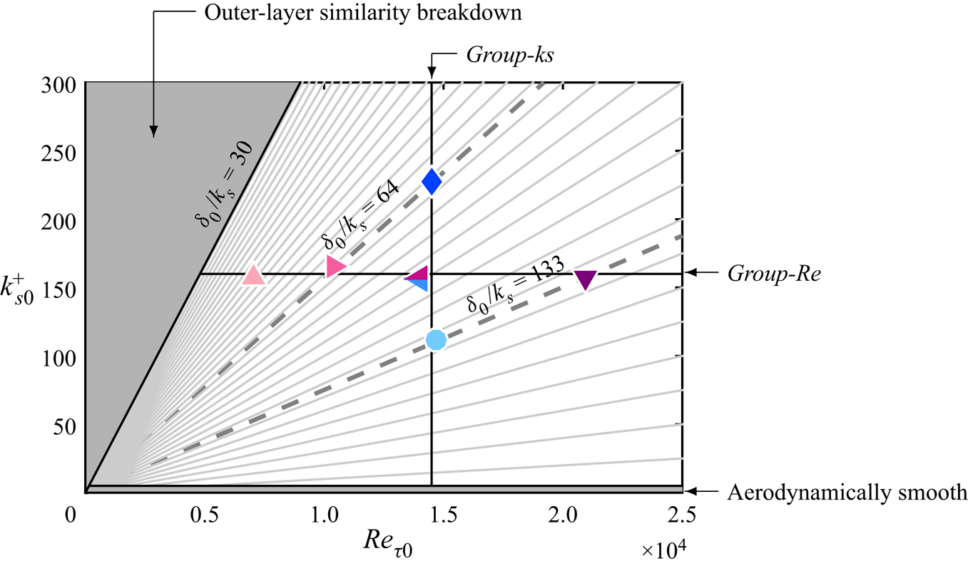
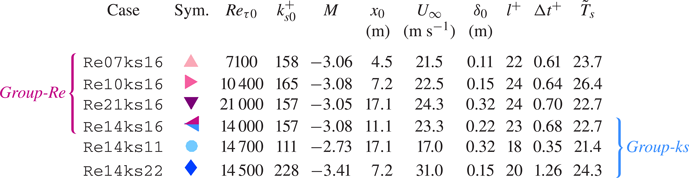
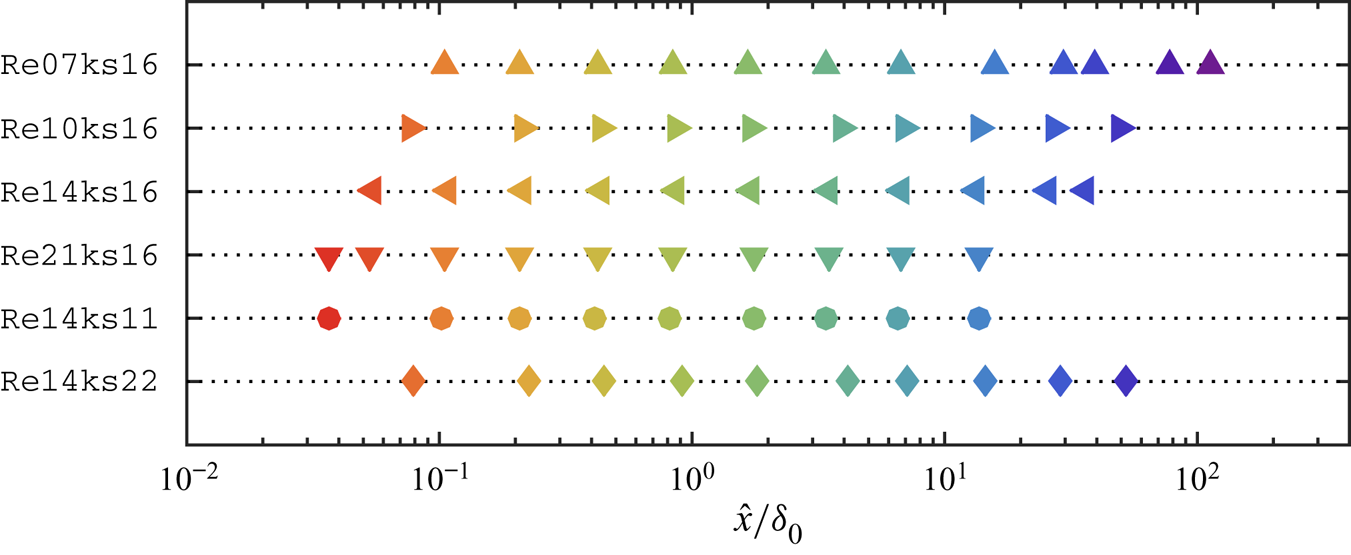
 $k_{s0}^{+}$. The aforementioned variation of flow parameters in each group is summarised in figure 2 and the relevant experimental conditions are listed in table 1. The streamwise length of the sandpaper,
 $x_0$, is more than 40 times greater than
 $\delta _0$ in the shortest case (Re07ks16), which is greater than the rough fetch used in many well-accepted studies (Antonia & Luxton Reference Antonia and Luxton1972; Hanson & Ganapathisubramani Reference Hanson and Ganapathisubramani2016, for instance), and the rough-to-smooth transition is sufficiently downstream of any expected tripping effects or inlet artefacts (Marusic et al. Reference Marusic, Chauhan, Kulandaivelu and Hutchins2015). It is also worth mentioning that
 $\delta _0/k_s$ is greater than 40 in all cases (see figure 2) and so the canonical outer-layer similarity is expected for the oncoming rough-wall boundary layers. Each case is assigned a code in the format of Rexxksyy, where xx
 $\approx Re_{\tau 0}/1000$, and yy
 $\approx k^{+}_{s0}/10$. Group-Re consists of cases Re07ks16, Re10ks16, Re14ks16 and Re21ks16, in which a nominally constant
 $k_{s0}^{+}\approx 160$ is maintained while
 $Re_{\tau 0}$ increases from 7100 to 21 000. Group-ks consists of cases Re14ks11, Re14ks16 and Re14ks22, in which a nominally constant
 $Re_{\tau 0} \approx 14000$ is maintained while
 $k_{s0}^{+}$ increases from 111 to 228. As shown in table 1, a unique symbol is assigned to each case, which will be adhered to throughout this paper (unless there are exceptions). All cases in Group-Re are represented by symbols with different shades of magenta, while cases in Group-ks are represented by symbols with different shades of blue. The shading of symbols darkens with increasing
 $Re_{\tau 0}$ in Group-Re and
 $k_{s0}^{+}$ in Group-ks. Note that case Re14ks16 is at the ‘crossing point’ in the parameter space so it is shared between two groups, therefore its symbol can take either pink or blue when plotted as part of the corresponding group.
Flow conditions ( $Re_{\tau 0}$ and
 $k_{s0}^{+}$) at the immediate upstream of the roughness transition of all cases. All symbols are defined in table 1. The horizontal line is at
 $k_{s0}^{+} = 160$, and the vertical line is at
 $Re_{\tau 0} = 14\,500$. Each light grey ray represents a combination of constant
 $\delta _0/k_s$, the reciprocal of which decreases from 0.033 (
 $\delta _0/k_s = 130$) to 0.001 (
 $\delta _0/k_s = 1000$) with a constant step of 0.001 in the clockwise direction. The two dashed lines show the cases with matched
 $\delta _{0}/k_s$ of 64 and 133.

Summary of the experimental cases. The friction velocity  $U_{\tau 0}$ employed in calculating
 $Re_{\tau 0}$ and
 $k^{+}_{s0}$ is obtained over the rough fetch just upstream of the rough-to-smooth transition. The viscous-scaled hotwire sensor length
 $l^{+}$ and the sampling interval
 ${\rm \Delta} t^{+}$ are calculated using the friction velocity at the most downstream measurement location on the smooth surface. Here,
 $\tilde {T}_s \equiv T_s U_{\infty }/\delta _{99}\times 10^{-3}$, where
 $T_s$ is the hotwire sampling time. Note that case Re14ks16 is shared between Group-Re and Group-ks, therefore its symbol can take either pink or blue colour in the corresponding group.

2.1. The facility
The experiments are performed in the High Reynolds Number Boundary Layer Wind Tunnel (HRNBLWT) at the University of Melbourne, which has a  $27\times 1.89\times 0.92$ m
 $^{3}$ working section (length
 $\times$ width
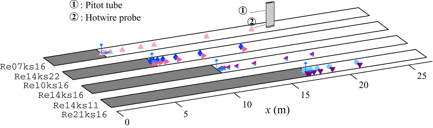
 $\times$ height), see the papers by Kulandaivelu (Reference Kulandaivelu2012) and Marusic et al. (Reference Marusic, Chauhan, Kulandaivelu and Hutchins2015) for further details. The overview of the experimental set-up is depicted in figure 3. An upstream portion of the tunnel floor in the test section is covered by P24 grit sandpaper (SP40F, Awuko Abrasives) from the inlet to the location of
 $x_0$ (as shown by the grey coloured patches in figure 3), while the remaining length is the original smooth aluminium surface. The sandpaper patch has a width of 1.82 m, covering nearly the entire width of the tunnel. By adjusting the bleeding slots on the tunnel roof, a nominal zero pressure gradient condition (
 $C_p(x)\equiv 1-(U_{\infty }(x)/U_{\textit{ref}})^{2}=0\pm 0.01$) is achieved, where
 $U_{{ref}}$ is obtained from an NPL (National Physical Laboratory) Pitot-static tube fixed in the free stream at
 $x = 0.7$ m from the tunnel inlet, and
 $U_{\infty }(x)$ from another Pitot-static tube mounted on the sting and traversed along the test section. To characterise the roughness parameters, a
 $60\ {\rm mm} \times 60\ {\rm mm}$ patch of the rough-to-smooth transition is scanned using an in-house-built laser scanner, which consists of a Keyence LK-031 laser triangulation sensor with a spot diameter of 0.03 mm and a linearity of 0.01 mm attached to an
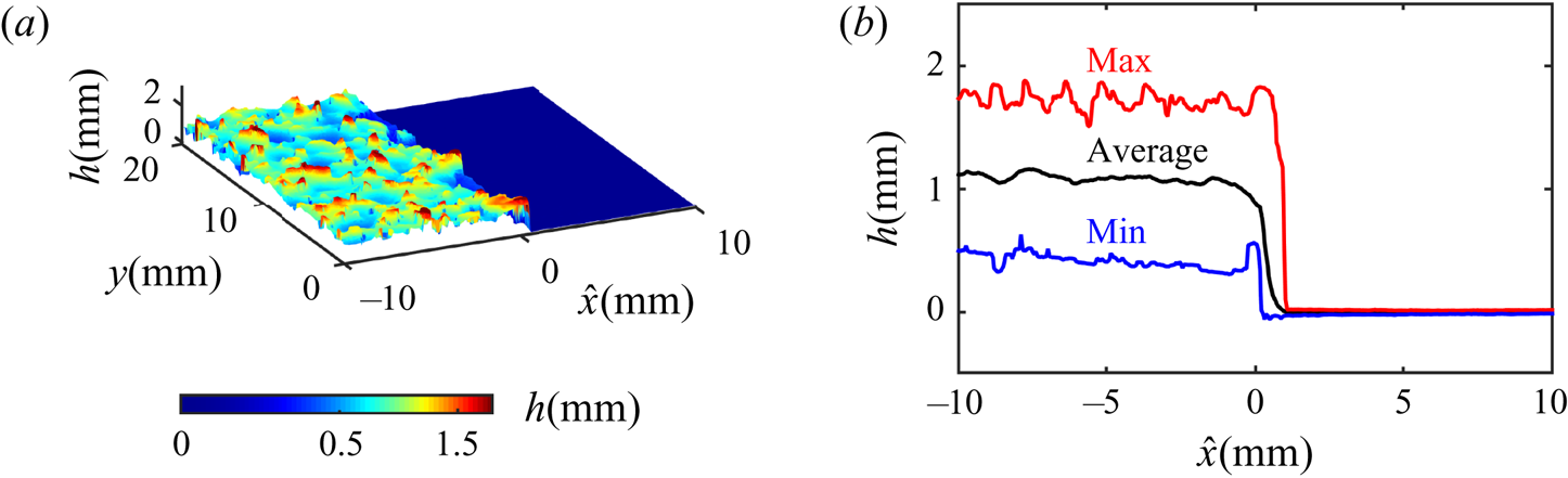
 $x - y$ traverse with a step size of 0.05 mm in both directions. The resulting surface topography is shown in figure 4. The smooth wall is approximately 1.8 mm below the roughness crest, i.e. the step height between the roughness crest and the smooth surface downstream is
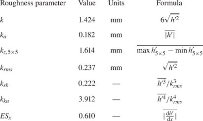
 ${\rm \Delta} H = -1.8\ \mathrm {mm}$. Detailed roughness parameters of the P24 sandpaper are listed in table 2.
Overview of the experimental set-up. The flow is going from the left to the right of the figure. The grey shaded surface represents the sandpaper, and the white region represents the smooth wall. Streamwise locations where a wall-normal hotwire profile is acquired in each case are shown by the corresponding symbols.

(a) The surface elevation at the rough-to-smooth transition measured using an in-house-built laser scanner. (b) The spanwise average of the surface elevation (black line), and the maximum (red line) and minimum (blue line) of the surface elevation along each spanwise line.

Roughness parameters from the scanned surface elevation of the P24 sandpaper. Here,  $h'\equiv h-\bar {h}$ is the surface deviation about the mean height, and
 $\max {h'_{5\times 5}}$ and
 $\min {h'_{5\times 5}}$ are the maximum and minimum of
 $h'$ in each of the
 $5\times 5$ tiles of the scanned surface (Thakkar, Busse & Sandham Reference Thakkar, Busse and Sandham2017).

2.2. Hotwire anemometry
A conventional single-wire hotwire probe is operated by an in-house-designed Melbourne University Constant Temperature Anemometer (MUCTA). To minimise aliasing, the hotwire signal is filtered using a Frequency Devices 9002 analogue filter with a cut-off frequency set to half of the sampling frequency. Digitisation of the resulting signal is via a Data Translation DT9836 data acquisition board with sampling frequency 50 kHz. The sampling parameters are summarised in table 1. The viscous-scaled sampling interval  ${\rm \Delta} t^{+}$ is less than 2 for all cases, which is safely below the threshold of
 ${\rm \Delta} t^{+}\approx 3$ to ensure a temporally well-resolved signal (Hutchins et al. Reference Hutchins, Nickels, Marusic and Chong2009). The hotwire sampling time
 $T_s$ is more than 20 000 boundary layer turn-over time (
 $\delta _{99}/U_{\infty }$) to achieve a good convergence of the statistics. Calibration is performed following an in situ procedure before and after each measurement. Thereafter, any drift is corrected by an intermediate single point re-calibration (ISPR) method discussed by Talluru et al. (Reference Talluru, Kulandaivelu, Hutchins and Marusic2014), where the hotwire voltage is periodically monitored in the free stream. The uncertainty in
 $U$ and
 $\overline {u^{2}}$ is usually within
 $1\,\%$ and
 $3\,\%$, respectively (Yavuzkurt Reference Yavuzkurt1984). The method of calibration drift correction proposed by Talluru et al. (Reference Talluru, Kulandaivelu, Hutchins and Marusic2014) employed here offers further improvements. During each run, the air temperature and atmospheric pressure data are also sampled to calculate
 $\nu$, the kinematic viscosity of air (Sutherland Reference Sutherland1893). The resulting
 $\nu$ varies from
 $1.51\times 10^{-5}$ to
 $1.64\times 10^{-5}$ m
 $^{2}$ s
 $^{-1}$ in different runs.
Velocity profiles are obtained by traversing a single-normal hotwire probe over 40 logarithmically spaced wall-normal locations from  $z/\delta _{99} \approx 0.001$ to 2. The sensing element of this probe has a diameter of
 $d = 2.5\ \mathrm {\mu }$m and a length-to-diameter ratio of 200. Note that in case Re14ks22 where
 $U_{\tau 0}$ is the highest among all cases, a wire with a smaller diameter (
 $d = 1.5\ \mathrm {\mu }$m) is used to maintain a similar spatial resolution in wall units (Hutchins et al. Reference Hutchins, Nickels, Marusic and Chong2009). Wall-normal boundary layer profiles are measured at over 10 logarithmically spaced streamwise locations downstream of the rough-to-smooth transition, from
 $\hat {x} = 12\ \mathrm {mm}$ to
 $x = 21\ \mathrm {m}$, as shown in figure 3 and also on a logarithmic axis in figure 5. The colour of each symbol in figure 5 is determined by its corresponding
 $\hat {x}/\delta _0$. This colour scheme will be used in the study of the streamwise evolution of the flow where a series of profiles at various streamwise locations are shown in one figure. A reference profile above the rough surface is also acquired at
 $\hat {x} = -0.1\ \mathrm {m}$ in each case. In order to accurately measure the wall location, a Renishaw RGH24 optical linear encoder with a resolution of 1
 $\mathrm {\mu }$m is used in the HRNBLWT. The initial offset is determined using a wall-normal traversing microscope equipped with a digital micrometer (CDI BG3600) with a resolution of 1
 $\mathrm {\mu }$m.
Downstream fetches where hotwire measurements are performed for all cases. The shape of each symbol indicates the case following the convention of table 1, while the colour reflects the magnitude of  $\hat {x}/\delta _0$.

2.3. Oil-film interferometry
The wall-shear stress  $\tau _w$ is directly measured using oil-film interferometry (OFI), which is one of the few methods available for a direct measurement at the surface with the required streamwise resolution to capture the rapid evolution following the rough-to-smooth transition. The technique measures the thinning rate of an oil film as it is being acted upon by the shear near the wall, which in turn permits an accurate measure of the mean wall-shear stress (Tanner & Blows Reference Tanner and Blows1976; Fernholz et al. Reference Fernholz, Janke, Schober, Wagner and Warnack1996; Zanoun, Durst & Nagib Reference Zanoun, Durst and Nagib2003). The thickness of a typical oil film is of the order of micrometres, which can be measured by the fringe pattern from the interference of light reflected from the top and bottom of the oil film. Moreover, the technique utilises inexpensive equipment, which includes a consumer camera and monochromatic light source (or a non-monochromatic light source with a bandpass filter).
The experimental procedure in this study follows a similar process as that described by Li et al. (Reference Li, de Silva, Baidya, Rouhi, Chung, Marusic and Hutchins2019). A 1.4 m long and 1 m wide glass insert has been installed in the tunnel floor at  $x = 5\ \mathrm {m}$, providing optical access from the underside of the tunnel for
 $\hat {x}/\delta _0 < 7$ in case Re07ks16. Both glass and aluminium surfaces are aerodynamically smooth. Steps between the glass insert and the aluminium wall are limited to 0.05 mm (2 wall units). The upstream joins between the glass and the aluminium floor are beneath the sandpaper. The OFI measurements are conducted on the centreline of the tunnel floor, therefore they are at a sufficient distance (
 ${>}5\delta _0$) away from these joins. This configuration provides a well-resolved fringe pattern with approximately 50 pixels per wavelength. A line of silicone oil is placed along the spanwise direction on the glass surface and spread downstream by the wind shear. The oil film is illuminated by an Imalent DX80 LED torch, and recorded using a Nikon D810 DSLR camera with a Tamron
 $180\ \mathrm {mm}$ macro lens. A
 $532\ \mathrm {nm}$ bandpass filter with a bandwidth of 10 nm is attached to the camera lens to obtain monochromatic fringe patterns. For the remaining measurements, a glass insert on the centreline of the working section ceiling provides optical access from above. To improve the fringe quality, the tunnel floor is covered by a piece of black mylar film with a thickness less than
 $40\ \mathrm {\mu }$m (equivalent to 1.5–2.5 wall units for all cases). This small step in the surface is at least 2 cm (
 ${>}500$ mylar film thicknesses,
 ${>}750$ wall units) away from the oil droplet in all directions except for the first few downstream locations, where the mylar film extends all the way to the rough-to-smooth change. The same illumination and imaging system as in the previous configuration is used, but with a reduced resolution of approximately 30 pixels per wavelength due to the
 $1\ \mathrm {m}$ stand-off distance between the camera and oil film. Both OFI configurations (imaging from underneath and above) have been compared at
 $\hat {x}/\delta _0 = 4$ for case Re07ks16, and are shown to give the same result to within
 $1\,\%$.
For both configurations, 100 images are captured with a time interval of five seconds in each measurement. The camera calibration and image processing algorithm are the same as detailed by de Silva et al. (Reference de Silva, Li, Baidya, Rouhi, Chung, Marusic and Hutchins2018).
3. Initial flow conditions on the rough surface
The streamwise evolution of the turbulent boundary layer starts from the initial flow condition on the rough surface. Once a rough-wall profile is specified, the flow recovery downstream on a smooth surface can be fully determined. A wall-normal hotwire profile is obtained at  $\hat {x} = -0.1$ m in each case to document the initial condition. For the hotwire measurements on the rough surface,
 $z = 0$ is located at the roughness crest following the method of measuring the initial offset as detailed by Squire et al. (Reference Squire, Morrill-Winter, Hutchins, Schultz, Klewicki and Marusic2016). Following the same study, the virtual origin of the roughness is assumed to be at the averaged surface elevation
 $\bar {h}=1.2$ mm (figure 4b), therefore a wall positioning correction of
 $\varepsilon ={\rm \Delta} H+\bar {h} = -0.6$ mm is used. In addition, Squire et al. (Reference Squire, Morrill-Winter, Hutchins, Schultz, Klewicki and Marusic2016) also demonstrated that for a similar type of sandpaper, varying the virtual origin from the roughness crest to the trough leads to a less than
 $0.8\,\%$ change in
 $U_{\tau }$ downstream of
 $x = 4.75$ m.
Nikuradse's (Reference Nikuradse1950) equivalent sand grain roughness  $k_s$ of the surface is obtained from the highest Reynolds number case Re21ks16 following the procedures below: first,
 $U_{\tau 0}$ on the rough surface is estimated by enforcing an outer-layer similarity (Townsend Reference Townsend1976) in the mean velocity deficit profile for
 $z/\delta _{99}>0.3$. The Hama function,
 ${\rm \Delta} U^{+}$, which is the vertical shift between the rough-wall profile and the logarithmic law
 $U^{+} = ({1}/{\kappa })\ln (z^{+})+B$, is then determined by minimising the least-squares error in the inertial range with the upper and lower bounds given by Mehdi, Klewicki & White (Reference Mehdi, Klewicki and White2013) and Squire et al. (Reference Squire, Morrill-Winter, Hutchins, Schultz, Klewicki and Marusic2016). The constants in the logarithmic law are chosen as
 $\kappa = 0.384$ and
 $B = 4.17$ (Nagib, Chauhan & Monkewitz Reference Nagib, Chauhan and Monkewitz2007). Finally,
 $k_{s0}^{+}$ is computed from
 ${\rm \Delta} U^{+}$ assuming Nikuradse's fully-rough relationship:
 \begin{equation} {\rm \Delta} U^{+} = \frac{1}{\kappa}\ln(k_{s0}^{+})+B-A'_{FR}, \end{equation}
where  $A'_{FR} = 8.5$ (Nikuradse Reference Nikuradse1950). The equivalent sand grain roughness is found to be
 $k_s \approx 2.43$ mm, which is approximately
 $1.7k$.
This  $k_s$ value is assumed for all other cases obtained with the same sandpaper. The rough-wall friction velocity
 $U_{\tau 0}$ is determined by minimising the difference between the Hama function obtained from the inner-normalised mean velocity profile and from the fully-rough relationship (3.1). The applicability of (3.1) can be justified in this case since all the rough-wall measurements are planned in the fully-rough regime with
 $k_{s0}^{+}>100$. Note that this method to determine
 $U_{\tau 0}$ from the measured mean velocity profile is similar to the approach described by Squire et al. (Reference Squire, Morrill-Winter, Hutchins, Schultz, Klewicki and Marusic2016). It is essentially a more informed modified Clauser chart method with
 $k_s$ (and therefore the relationship between
 ${\rm \Delta} U^{+}$ and
 $U_{\tau 0}$) prescribed. The
 ${\rm \Delta} U^{+}$ and
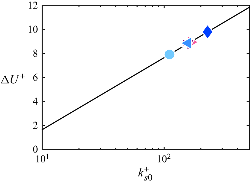
 $k_{s0}^{+}$ for all cases determined by this approach are shown in figure 6. In Group-ks where the effect of
 $k_{s0}^{+}$ is studied,
 $k_{s0}^+$ varies from 111 to 228, which corresponds to a range of
 ${\rm \Delta} U^{+}$ from 7.9 to 9.8.
Hama function,  ${\rm \Delta} U^{+}$, as a function of the inner-scaled equivalent sand grain roughness
 $k_{s0}^+$ for all cases. All symbols are defined in table 1 with the colour indicating
 $Re_{\tau 0}$ or
 $k_{s0}^{+}$, and the solid line is Nikuradse's fully-rough relationship as shown in (3.1).

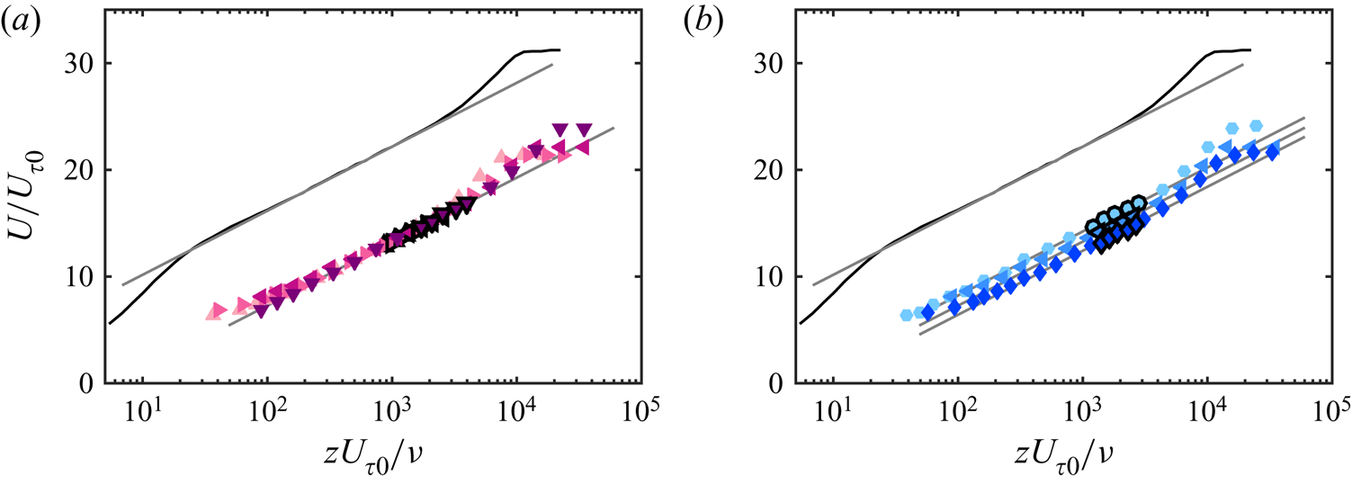
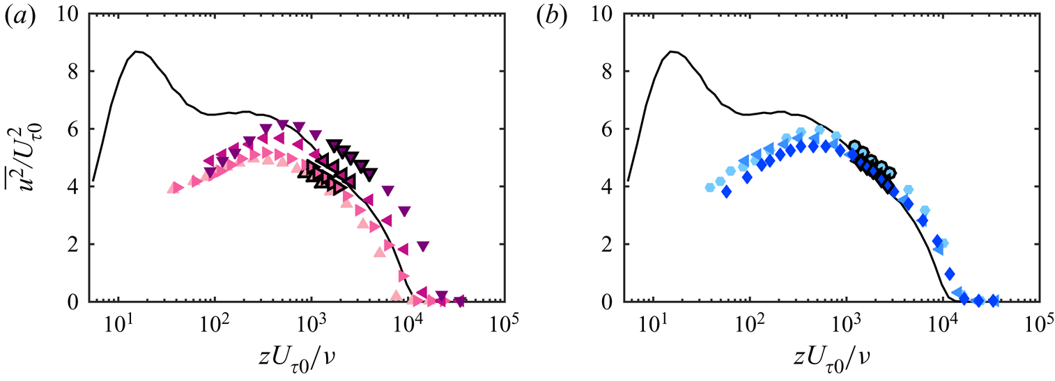
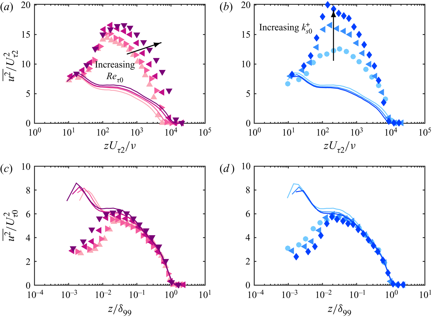
Figures 7 and 8 respectively show the inner-normalised mean streamwise velocity and turbulence intensity profiles of both Group-Re (a) and Group-ks (b) just upstream of the roughness transition at  $\hat {x} = -0.1$ m. As expected, a good collapse of the data in the logarithmic region in figure 7(a) indicates that
 ${\rm \Delta} U^{+}$ (and therefore
 $k_{s0}^{+}$) in Group-Re are closely matched, whereas the vertical shifts in the velocity profile in figure 7(b) correspond to the
 $k_{s0}^{+}$ trend as planned for Group-ks. Similarly the
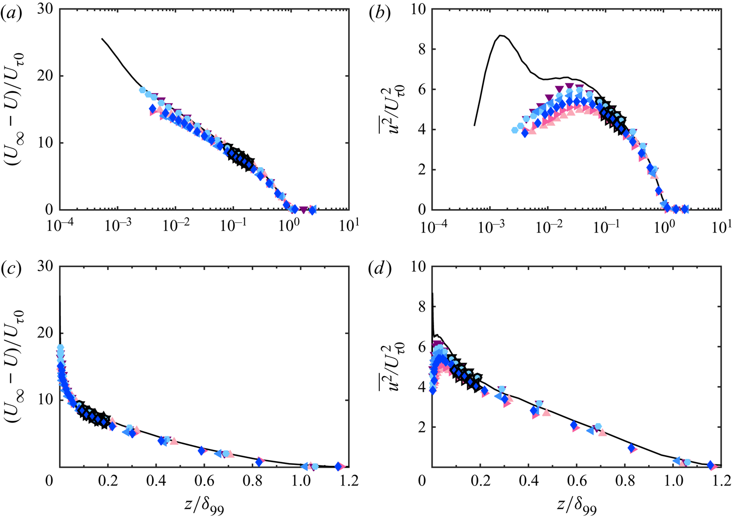
 $Re_{\tau 0}$ trend can be observed in figures 7(a) and 8(a). Townsend's outer-layer similarity hypothesis (Townsend Reference Townsend1976) appears to be nominally satisfied as shown by the outer-normalised profiles for both groups in figure 9, in agreement with previous studies of three-dimensional roughness (for example Flack, Schultz & Shapiro Reference Flack, Schultz and Shapiro2005; Wu & Christensen Reference Wu and Christensen2007; Squire et al. Reference Squire, Morrill-Winter, Hutchins, Schultz, Klewicki and Marusic2016). Overall, these results demonstrate that the rough-wall profiles immediately upstream of the roughness transition exhibit similar behaviours as a turbulent boundary layer developed on a homogeneously rough surface in a quasi-equilibrium state.
Inner-normalised mean streamwise velocity profiles at  $\hat {x} = -0.1$ m from (a) Group-Re and (b) Group-ks. The black line in both figures is a smooth-wall reference profile with
 $Re_{\tau } = 1.0\times 10^{4}$ acquired in the same facility using hotwire anemometry and normalised using the corresponding smooth-wall friction velocity (Marusic et al. Reference Marusic, Chauhan, Kulandaivelu and Hutchins2015). The colour of the symbols indicates (a)
 $Re_{\tau 0}$ and (b)
 $k_{s0}^{+}$, as defined in table 1. Symbols with a black outline represent the extent of the inertial range. These data points are employed in the fit to obtain
 $U_{\tau 0}$. Only every second data point is shown for clarity except in the inertial range.

Inner-normalised streamwise turbulence intensity profiles at  $\hat {x} = -0.1$ m from (a) Group-Re and (b) Group-ks. Legends are the same as in figure 7.

(a) Mean streamwise velocity deficit and (b) streamwise turbulence intensity versus outer-normalised wall-normal distance for both Group-Re and Group-ks. The corresponding plots with a linear  $x$-axis are shown as (c,d). Legends are the same as in figure 7.

4. Skin-friction coefficient
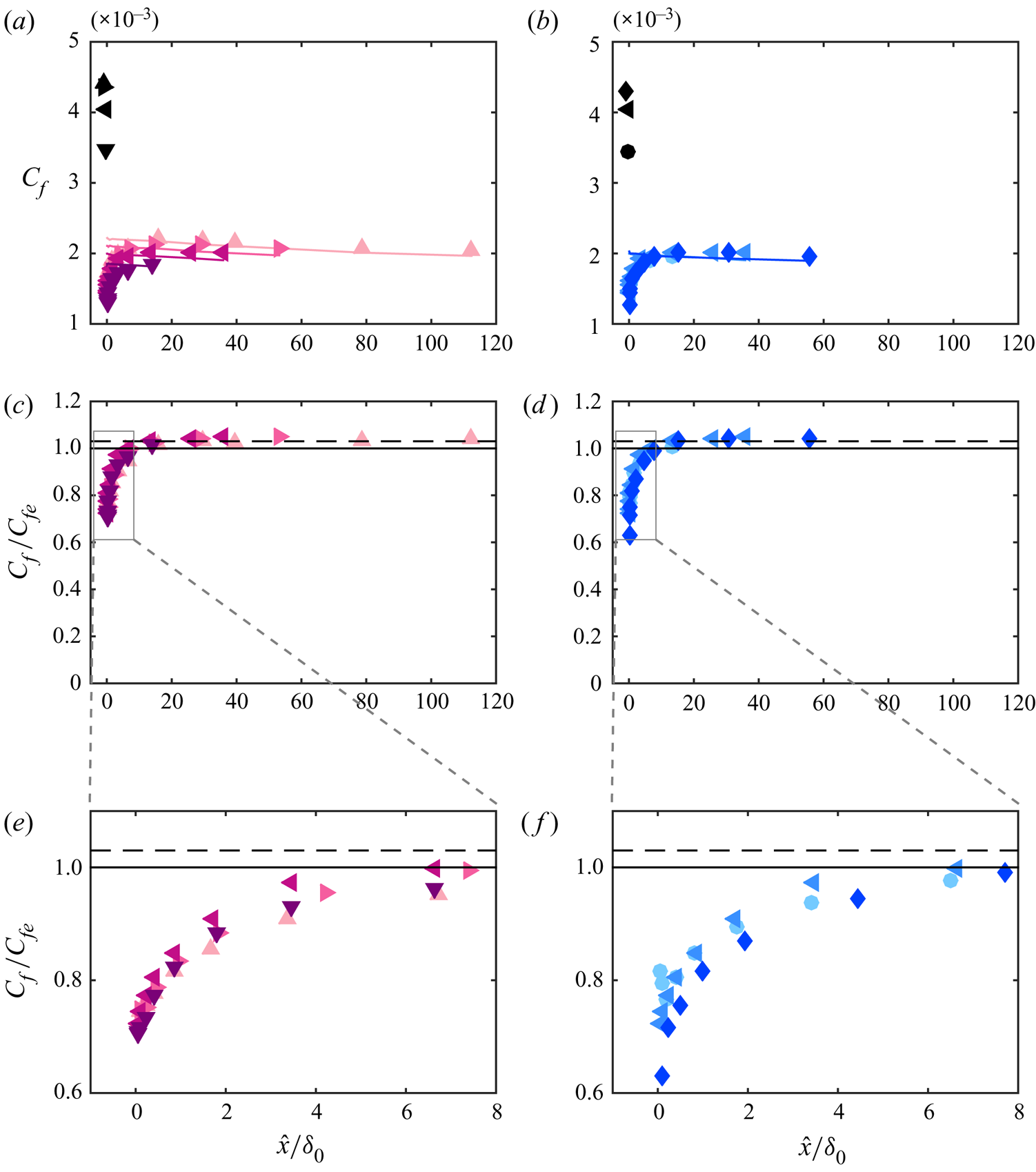
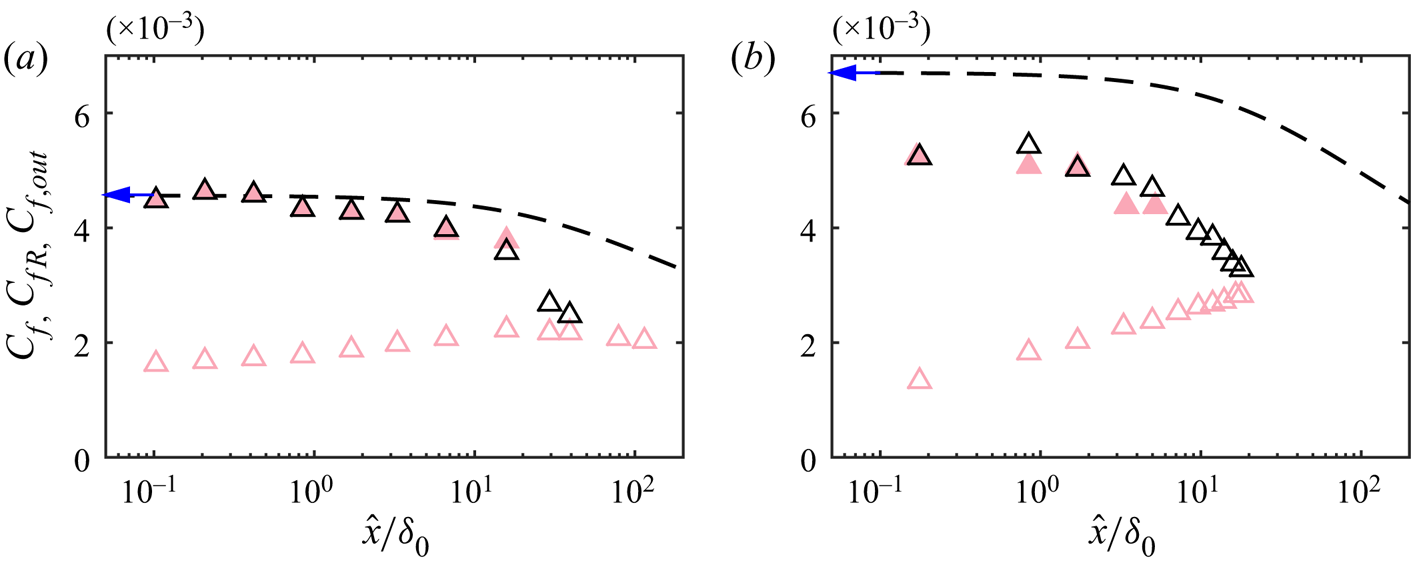
We first examine the recovery of the skin-friction coefficient downstream of the rough-to-smooth change for all cases. Figure 10(a,b) show the evolution of  $C_f$ following the rough-to-smooth transition of Group-Re and Group-ks cases, respectively. Over the smooth surface,
 $C_f$ is measured directly using OFI (shown by the coloured symbols in figure 10a,b), and the reference
 $C_f$ over the rough surface (black symbols) is calculated from the mean velocity profile following the method detailed in § 3. In all cases,
 $C_f$ undershoots the expected equilibrium smooth-wall value (shown by the solid lines) immediately downstream of the roughness transition, then reaches its maximum at
 $\hat {x}/\delta _0\approx 20$ before decreasing gradually farther downstream as dictated by the increasing Reynolds number of the flow. The black symbols show
 $C_f$ on the rough surface just upstream of the surface transition. In all cases there is a three- to five-fold decrease in
 $C_f$ immediately downstream of the transition. When comparing
 $C_f$ between cases in Group-Re, we notice that
 $C_f$ on both rough and smooth surfaces decreases with
 $Re_{\tau 0}$ as evident in figure 10(a). Such a dependence on
 $Re_{\tau 0}$ is expected and is similar to that observed for a turbulent boundary layer on a homogeneous surface (e.g. Nagib et al. Reference Nagib, Chauhan and Monkewitz2007). For Group-ks measurements on the other hand,
 $C_f$ increases with
 $k_{s0}^{+}$ only on the rough surface (as shown by the solid black symbols in figure 10b). The smooth-wall
 $C_f$ from all three cases collapse to a single trend, as these cases have very similar
 $Re_{\tau }$ values on the smooth wall, and the
 $C_f$ of the fully recovered flow is solely determined by the local
 $Re_{\tau }$.
Skin-friction coefficient  $C_f$ versus the fetch
 $\hat {x}$ over the downstream smooth surface scaled by
 $\delta _0$ for (a) Group-Re and (b) Group-ks. The coloured symbols represent OFI measurements on the smooth wall, and the black symbols are obtained from the reference profile over the rough surface. The solid lines show
 $C_{fe}$, the expected equilibrium smooth-wall skin-friction coefficient at every streamwise location. (c,d)
 $C_f$ normalised by its equilibrium value
 $C_{fe}$ for Group-Re and Group-ks, respectively, with the corresponding magnified view of the boxed region shown in (e,f). The colour of the symbols and solid lines indicates
 $Re_{\tau 0}$ and
 $k_{s0}^{+}$ in the left and right column, respectively, as defined in table 1. The solid horizontal line is
 $C_f/C_{fe} = 1$, and the dashed line is
 $C_f/C_{fe} = 1.03$.

The expected equilibrium skin-friction coefficient,  $C_{fe}$, is defined as the skin-friction coefficient that an equilibrium turbulent boundary layer at the same Reynolds number (based on momentum thickness) would have (Hanson & Ganapathisubramani Reference Hanson and Ganapathisubramani2016). The
 $C_{fe}$ is estimated using an empirical relationship obtained from drag balance measurements of a smooth-wall turbulent boundary layer in the same facility (Baars et al. Reference Baars, Squire, Talluru, Abbassi, Hutchins and Marusic2016):
 \begin{equation} C_{fe} = 2\left(\ln \left(Re_{\theta}\right)/0.38+3.7\right)^{{-}2}, \end{equation}
where  $Re_{\theta }\equiv U_{\infty } \theta /\nu$, and
 $\theta$ is the momentum thickness computed locally by integrating the measured mean velocity profile. If the flow has fully recovered to the smooth-wall condition, then
 $C_{f}$ should equal to
 $C_{fe}$. Therefore, it can serve as an indication of the flow recovery. Similar to
 $C_f$ at a large fetch,
 $C_{fe}$ also decreases with increasing
 $Re_{\tau 0}$ (therefore increasing
 $Re_{\theta }$) in Group-Re. As a consequence of the matched
 $Re_{\tau 0}$, Group-ks cases have similar
 $Re_{\theta }$ downstream of the rough-to-smooth change, which leads to the agreement in
 $C_{fe}$ between cases.
The recovery of  $C_f$ towards
 $C_{fe}$ is further examined through the ratio
 $C_f/C_{fe}$ in figure 10(c,d). Immediately downstream of the rough-to-smooth transition,
 $C_f$ is approximately 60 %–80 % of
 $C_{fe}$ for all cases, followed by a quick recovery to
 $C_{fe}$ within approximately
 $20\delta _0$. The data points overshoot
 $C_{f}/C_{fe} = 1$ (the black horizontal line) slightly and then reach a plateau at
 $C_{f}/C_{fe} = 1.03$. This 3 % difference is possibly related to the uncertainty in the data and the empirical relationship (4.1) employed. Regardless, there seems to be little difference between cases in both Group-Re and Group-ks in terms of the
 $C_f$ recovery behaviour when scaled by
 $\delta _0$ and
 $C_{fe}$ in the far field. When normalised by
 $C_{fe}$, as shown in figure 10(c,d), to within the experimental uncertainty,
 $C_f$ evolves as if the flow were in quasi-equilibrium with the smooth wall beyond
 $\hat {x}/\delta _0\approx 20$. Utilising two different types of roughness (grit and mesh), Hanson & Ganapathisubramani (Reference Hanson and Ganapathisubramani2016) achieved a more than five-fold change in
 $k_{s0}^{+}$, and they reported a decrease in the recovering
 $C_f$ with increasing
 $k_{s0}^{+}$. This range of
 $k_{s0}^{+}$ is unfortunately not attainable without physically increasing the equivalent sand-grain roughness
 $k_s$, and we do not observe a trend with
 $k_{s0}^{+}$ in
 $C_f$ as a result of the limited
 $k_{s0}^{+}$ range in this study. For a larger range of
 $k_{s0}^{+}$ (larger perturbation strength
 $|M|$) we would expect to see an influence on
 $C_f$ recovery. However, it is interesting to note that in both studies the full recovery of
 $C_f$ to the smooth-wall value is found at a streamwise fetch of
 $\hat {x}/\delta _0\approx 20$.
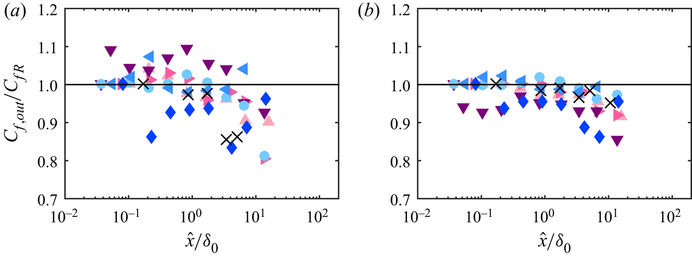
The scatter in  $C_f$ close to the roughness transition between cases appears to be more prominent in Group-ks compared with Group-Re as revealed by the magnified view in figure 10(e,f). As the step height between the roughness crest and the smooth surface
 ${\rm \Delta} H = -1.8\ \mathrm {mm}$ is the same for all cases in both groups, this trend in
 $C_f$ might be dependent on the inner-normalised step height
 ${\rm \Delta} H^{+}$, which increases with
 $k_{s0}^{+}$ (effectively
 $U_{\tau 0}/\nu$) in the current implementation. It has also been shown by OFI measurements using a spanwise line of silicone oil at a comparable Reynolds number that the local distribution of roughness elements can have an effect on
 $C_f$ in the range of
 $\hat {x}/\delta _0<0.4$ (Li et al. Reference Li, de Silva, Baidya, Rouhi, Chung, Marusic and Hutchins2018). This might also be responsible for some of the variation in
 $C_f$ in the extreme near field (
 $0 < \hat {x}/\delta _0 < 0.4$) as the local roughness geometry (at an element scale) on the centreline of the tunnel floor (where the OFI measurements are performed) varies between cases where a different piece of sandpaper is used.
5. Internal boundary layer
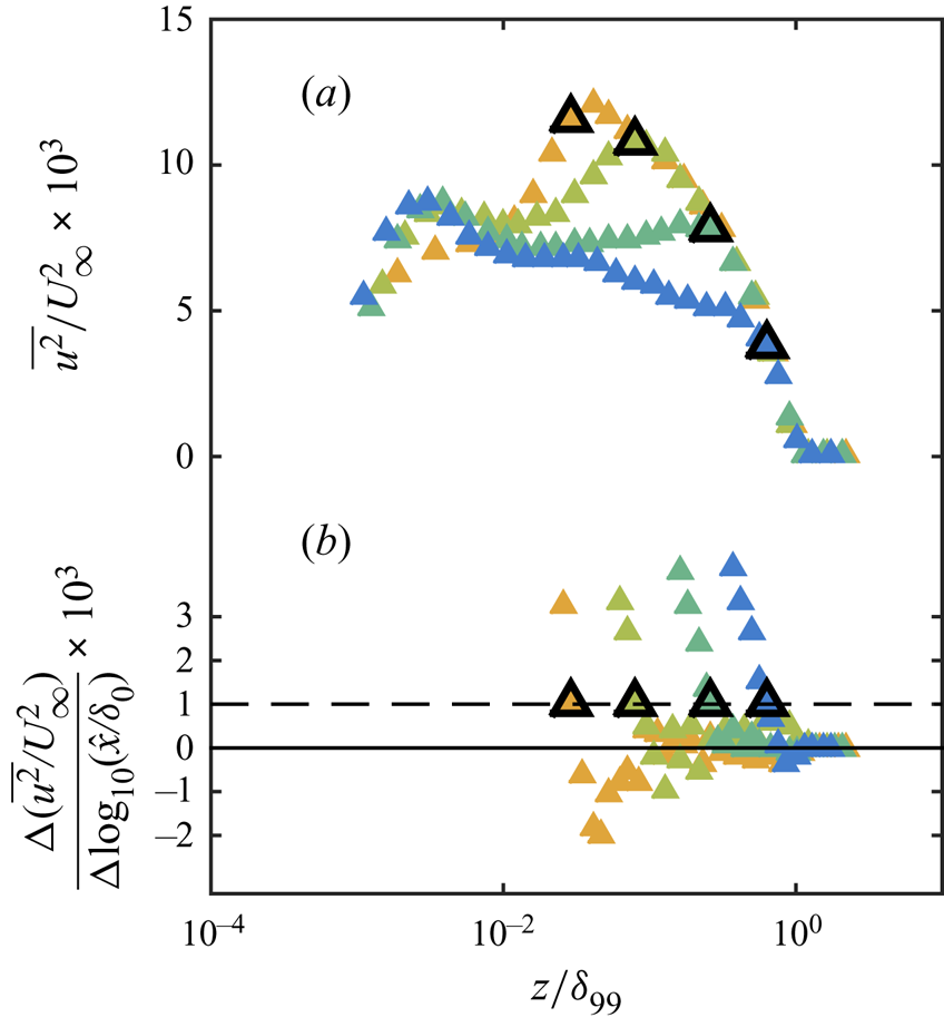
The extent of flow recovery can also be quantified by the growth of the IBL. The IBL height  $\delta _i$ at each streamwise location is calculated based on the difference between the
 $\overline {u^{2}}/U^{2}_{\infty }$ profile at the current location and the neighbouring upstream measurement location, i.e.
 $\delta _i$ is defined as the wall-normal location where
 $\partial (\overline {u^{2}}/U^{2}_{\infty })/\partial x \rightarrow 0$. It is well-known that in a canonical boundary layer with no surface heterogeneity,
 $\overline {u^{2}}$ exhibits outer-layer similarity only when normalised by
 $U_{\tau }^{2}$, and a dependence on Reynolds number presents if the velocity scale
 $U_{\infty }$ is used instead. However, the adequacy of this approach can be justified considering that the largest change of Reynolds number between the neighbouring profiles used to compute
 $\delta _i$ is usually within
 $10\,\%$, and the difference in the Reynolds number is negligible close to the roughness transition. The majority of the measurements are concentrated in this region owing to the logarithmic streamwise spacing employed for these measurements. It has been shown that
 $\delta _i$ determined from the turbulence intensity profile is comparable with the results from the more conventional methods based on the mean velocity profiles (Pendergrass & Arya Reference Pendergrass and Arya1984; Li et al. Reference Li, de Silva, Baidya, Rouhi, Chung, Marusic and Hutchins2019; Rouhi et al. Reference Rouhi, Chung and Hutchins2019a). Here we favour the turbulence intensity approach as the distinction associated with the roughness change is more pronounced in
 $\overline {u^{2}}$ compared with
 $U$ and less subject to small uncertainties in the measurement, resulting in a more robust estimation of
 $\delta _i$. Figure 11 illustrates the process of extracting
 $\delta _i$ from the outer-scaled turbulence intensity profiles. Figure 11(a) shows good collapse in the outer layer with no appreciable Reynolds number trend, and the decrease in the turbulence intensity related to the internal layer growth is much more pronounced compared with the negligible Reynolds number trend. Figure 11(b) shows the difference between two consecutive outer-scaled turbulence intensity profiles
 ${\rm \Delta} (\overline {u^{2}}/U^{2}_{\infty })$ divided by
 ${\rm \Delta} \log _{10}(\hat {x}/\delta _0)$, the difference in the logarithmic fetch of these two streamwise locations. We use this difference to extract the IBL height
 $\delta _i$. In practice, a threshold of
 ${\rm \Delta} (\overline {u^{2}}/U^{2}_{\infty })/{\rm \Delta} \log _{10}(\hat {x}/\delta _0) = 1\times 10^{-3}$ rather than 0 is selected to account for the noise in measurements. Note that there is also a weak Reynolds number trend in
 $\overline {u^{2}}/U^{2}_{\infty }$ profiles with increasing fetch: considering a rough-wall turbulent boundary layer satisfying the outer-layer similarity hypothesis, i.e.
 $\overline {u^{2}}/U^{2}_{\tau } = f(z/\delta _{99})$, the streamwise difference
 ${\rm \Delta} (\overline {u^{2}}/U^{2}_{\infty })/{\rm \Delta} \log _{10}(\hat {x}/\delta _0) =f(z/\delta _{99}){\rm \Delta} C_f/(2{\rm \Delta} \log _{10}(\hat {x}/\delta _0))$, which is around
 $3\times 10^{-4}$ or less. Therefore, with the current approach, the weak Reynolds number trend has insignificant effect on the
 $\delta _i$ results, especially in the near field. To examine the sensitivity of the resulting
 $\delta _i$ to the threshold, we reprocess the data of case Re07ks16 with a threshold of
 $2\times 10^{-3}$. Doubling the threshold leads to an underestimation up to 15 % in
 $\delta _i$ compared with that with a threshold of
 $1\times 10^{-3}$. The exponent of a power-law fit through the data (to be discussed below) is changed from 0.77 to 0.75. In summary, doubling the threshold leads to a smaller
 $\delta _i$, but the general trend of the data remains little changed. This method of extracting
 $\delta _i$ tends to pick up the upper edge of the modified region. In the vicinity of the rough-to-smooth change (
 $\hat {x}/k\lesssim 10$), this method could presumably detect the upper limit of the roughness trailing wake (see figure 1).
(a) Streamwise turbulence intensity of case Re07ks16 normalised by  $U_{\infty }$, plotted against the outer-scaled wall-normal location
 $z/\delta _{99}$. (b) The difference between two consecutive (in
 $x$)
 $\overline {u^{2}}/U_{\infty }^{2}$ profiles close to the edge of the IBL, plotted on the same abscissa. In both figures, shading of the symbols indicates the fetch with the colour scheme detailed in figure 5. The four profiles in this figure are obtained at
 $\hat {x}/\delta _0 = 0.2,0.8,3.4$ and 15.7. Note that turbulence intensity profiles are shown only at every second streamwise location measured for clarity. The symbols with thick black outlines represent the location of the edge of the IBL. The solid horizontal line in (b) is at
 ${\rm \Delta} (\overline {u^{2}}/U_{\infty }^{2})/{\rm \Delta} \log _{10}(\hat {x}/\delta _0) = 0$, and the dashed line shows the threshold
 ${\rm \Delta} (\overline {u^{2}}/U_{\infty }^{2})/{\rm \Delta} \log _{10}(\hat {x}/\delta _0) = 1\times 10^{-3}$.

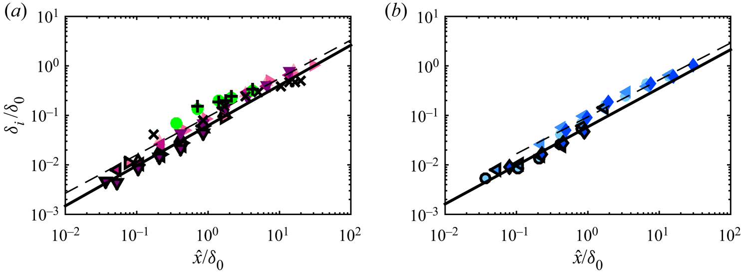
Using the method described above,  $\delta _i$ at various streamwise locations is calculated for all cases and presented in figure 12. Both
 $\delta _i$ and
 $\hat {x}$ are normalised by
 $\delta _0$, the boundary layer thickness at the rough-to-smooth transition. All data points collapse on to a straight line in logarithmic scale with no distinguishable trend with
 $Re_{\tau 0}$ or
 $k_{s0}^{+}$. A power-law fit
 \begin{equation} \delta_i/\delta_{0} = A_0 (\hat{x}/\delta_0)^{b_0} \end{equation}
results in coefficients of  $A_0 = 0.094$ and
 $b_0 = 0.77$ for Group-Re, and
 $A_0 = 0.095$ and
 $b_0 = 0.75$ for Group-ks. This agrees closely with the observations of Bradley (Reference Bradley1968) and Mulhearn (Reference Mulhearn1978), where
 $\delta _i$ is defined as the ‘merging point’ in the mean velocity profile. The growth appears to be more aggressive than
 $\delta _i\propto \hat {x}^{0.43}$ as reported by Antonia & Luxton (Reference Antonia and Luxton1972). The major differences are: in their study, (1)
 $\delta _i$ is defined as the inflection point in the
 $U$ versus
 $z^{1/2}$ plot and (2) the upstream surface is roughened by two-dimensional square ribs instead of sandpaper. In order to further clarify the underlying reason behind the disparity between these two results, we present
 $\delta _i$ estimated from the present dataset using the same definition as used by Antonia & Luxton (Reference Antonia and Luxton1972). The resulting
 $\delta _i$ is shown in figure 12 by symbols with the corresponding shape and colour but with a thick black outline. Note that we only show the data points where
 $\delta _i/\delta _{99}<0.15$ is satisfied to eliminate the contamination from the wake profile in this method. A power-law fit through the data points in each group is also shown in the figure by a thick solid line. The fitting coefficients are
 $A_{0} = 0.062$ and
 $b_{0} = 0.81$ for Group-Re, and
 $A_{0} = 0.059$ and
 $b_{0} = 0.78$ for Group-ks. Thus the
 $\delta _i$ calculated using Antonia and Luxton's definition appears to be lower than the results obtained by thresholding the variance profile. This is expected as the former definition returns the ‘mid-point’ of a dispersed or fluctuating IBL, while the current definition is more likely to pick up its upper limit. Regardless, exponents from the power-law fits of both Group-Re and Group-ks using Antonia and Luxton's definition for
 $\delta _i$ are approximately 0.8, which is very close to the result using the current variance-based definition. In fact, the power-law exponent itself is a very sensitive quantity to assess. The streamwise extent where the fit is performed, the noise and scatter in the data points, and the step height effect at small fetches (see Rouhi et al. Reference Rouhi, Chung and Hutchins2019b, for example) can all affect the resulting power-law exponent. As shown by the green symbols in figure 12(a), the
 $\delta _i$ versus
 $\hat {x}$ trend of Antonia & Luxton (Reference Antonia and Luxton1972) is very similar to that in the present study. Note that in the study by Antonia & Luxton (Reference Antonia and Luxton1972), the data point at
 $\hat {x}/\delta _0 \approx 0.4$ (
 $\hat {x} = 1\ \mathrm {in}$) is omitted from the fit. A fit through all available data points will potentially bring the exponent closer to 0.8. In addition, the black crosses in figure 12(a) are
 $\delta _i$ of the grit case in the study by Hanson & Ganapathisubramani (Reference Hanson and Ganapathisubramani2016), which is also determined following Antonia and Luxton's definition. They are observed to follow the trend in the current data except for the undershoot in the far field, where
 $\delta _i$ is presumably in the wake region. To conclude, the power-law exponents of
 $\delta _i$ determined from both variance and
 $U$ versus
 $z^{1/2}$ profiles are very similar, although the latter gives a slightly lower multiplicative coefficient
 $A_0$ as dictated by the nature of the method. The growth trends of
 $\delta _i$ in the current study are comparable with the past works, including those with a seemingly different power-law exponent. The underlying reason is that the power-law exponent is very sensitive to noise or uncertainty in
 $\delta _i$, especially when the data points are few, or the power law fit is conducted over a limited range of
 $\hat {x}/\delta _0$.
IBL thickness  $\delta _i$ versus the fetch
 $\hat {x}$ over the downstream smooth surface, both normalised by
 $\delta _0$, the boundary layer thickness at the roughness transition (coloured symbols without outlines). The symbols with a thick black outline are
 $\delta _i$ calculated using the same definition as used by Antonia & Luxton (Reference Antonia and Luxton1972). The colour of the symbols indicates (a)
 $Re_{\tau 0}$ and (b)
 $k_{s0}^{+}$, as defined in table 1. The thin dashed line is (5.1), a power-law fit through
 $\delta _i$ calculated from the variance profile using the present method, and the thick solid line is a power-law fit through
 $\delta _i$ calculated using the definition of Antonia & Luxton (Reference Antonia and Luxton1972). For comparison,
 $\delta _i$ reported in the original study of Antonia & Luxton (Reference Antonia and Luxton1972) is shown in (a), where the black pluses and green dots represent
 $\delta _i$ determined as the inflection point in the
 $U$ versus
 $z^{1/2}$ profile and the ‘merging point’ in the neighbouring mean velocity profiles where
 ${\rm \Delta} U=0$, respectively. The black crosses are
 $\delta _i$ determined from the
 $U$ versus
 $z^{1/2}$ profile of the grit case of Hanson & Ganapathisubramani (Reference Hanson and Ganapathisubramani2016).

Based on the fitted power law, the downstream fetch required for the IBL to reach the local  $\delta _{99}$ is estimated to be
 $\hat {x}/\delta _0 = 26.5$, which is at approximately the same location as where the maximum of
 $C_f$ occurs (see figure 10a,b). However, we would like to re-emphasise that here we adopt the definition of the IBL as the region where the flow is modified by the new wall condition, and the flow within the IBL has been shown to be in a non-equilibrium state with the local wall conditions (see Antonia & Luxton Reference Antonia and Luxton1971; Li et al. Reference Li, de Silva, Baidya, Rouhi, Chung, Marusic and Hutchins2019; Rouhi et al. Reference Rouhi, Chung and Hutchins2019a). This implies that even when
 $\delta _i \rightarrow \delta _{99}$ (when the internal layer has grown to the full layer height), the boundary layer may still not be in full quasi-equilibrium with the new wall condition. A complete recovery of all flow statistics to the quasi-equilibrium state is expected at a longer fetch, as will be evidenced in the following sections.
6. Mean streamwise velocity
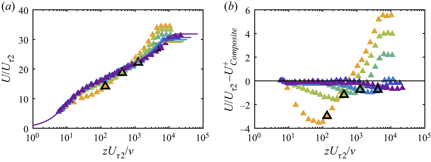
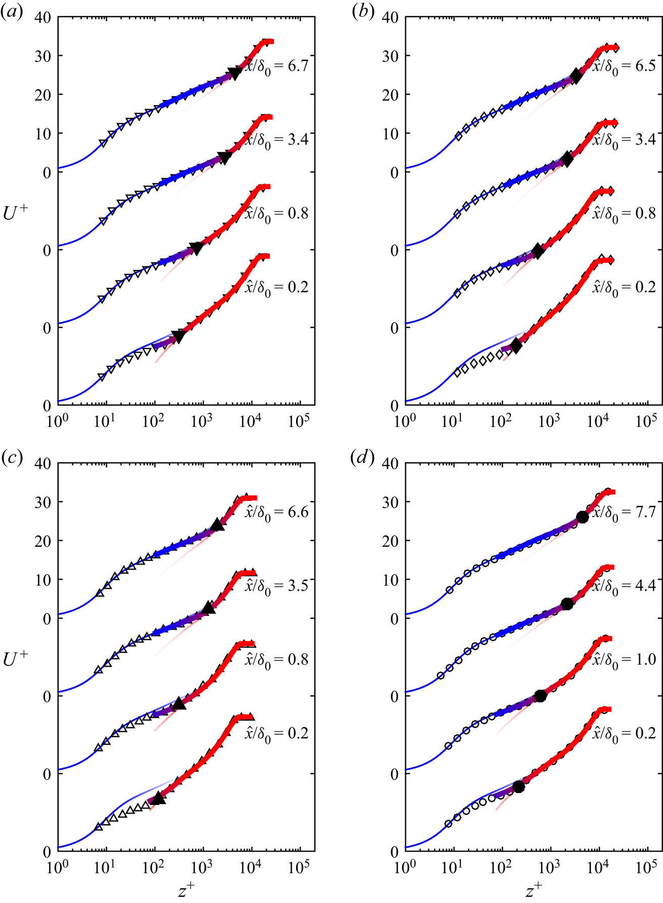
We utilise the hotwire data to further investigate the recovery of the mean flow statistics. We will primarily present the results of case Re07ks16 as it permits the greatest streamwise development downstream of the roughness transition (hence demonstrating the asymptotic trends more clearly); however, very similar trends are observed in other cases and are not shown here for brevity. Mean streamwise velocity profiles normalised by the local  $U_{\tau 2}$ over the smooth wall measured using OFI are shown in figure 13(a). The coloured lines in the figure are composite velocity profiles at matched
 $Re_{\tau }$, following the expression of Chauhan et al. (Reference Chauhan, Monkewitz and Nagib2009). They represent a reference at a quasi-equilibrium state with the smooth surface. The measured mean velocity profile overshoots the corresponding composite profile in the wake region, and this overshoot (the wake strength) diminishes with the downstream fetch as dictated by the recovering
 $C_f$ (see figure 10), approaching the smooth-wall reference. The recovery of the flow at different wall-normal locations occurs at different rates: as shown in figure 13(a), the mean velocity profile in the buffer region conforms to the smooth-wall reference after a short fetch of
 $\hat {x}/\delta _0=3.4$, while it takes
 $\hat {x}/\delta _0\gtrsim 20$ for the wake region to recover.
(a) Inner-normalised mean velocity profile for case Re07ks16. The solid coloured lines are composite profiles computed at matched  $Re_{\tau }$ following Chauhan, Monkewitz & Nagib (Reference Chauhan, Monkewitz and Nagib2009). (b) The difference between the measured mean streamwise velocity
 $U$ normalised by the local friction velocity
 $U_{\tau 2}$ and the composite profile
 $U^{+}_{{Composite}}$ for the same case. In both figures, shading of the symbols changes from yellow to green and then to violet as the fetch increases. The colour scheme is summarised in detail in figure 5. The profiles shown in the figure are obtained at
 $\hat {x}/\delta _0 = 0.2,0.8,3.4,15.7,39.4$ and 112. The symbols with thick black outlines show the location of the IBL (detailed in § 5) in each profile. Note that the mean velocity profiles are shown only at every second streamwise location measured for clarity.

The locations of the IBL in each profile as determined in § 5 are shown by the symbols with thick black outlines. The measured mean velocity profiles exhibit a good collapse with the reference composite profile at  $z^{+}<10$; however, there is a general lack of agreement in the buffer region and beyond, despite the fact that this region is well below the edge of the IBL. This confirms that the flow within the IBL is not in equilibrium with the local wall condition (Antonia & Luxton Reference Antonia and Luxton1972; Ismail et al. Reference Ismail, Zaki and Durbin2018; Li et al. Reference Li, de Silva, Baidya, Rouhi, Chung, Marusic and Hutchins2019; Rouhi et al. Reference Rouhi, Chung and Hutchins2019a). The deviation from the smooth-wall composite profile is better demonstrated by viewing the velocity difference
 $U/U_{\tau 2}-U^{+}_{{Composite}}$ shown in figure 13(b). The difference between the measured profile and the smooth-wall reference persists even beyond
 $\hat {x}/\delta _0>10$ in the logarithmic region (see light blue symbols in figure 13b).
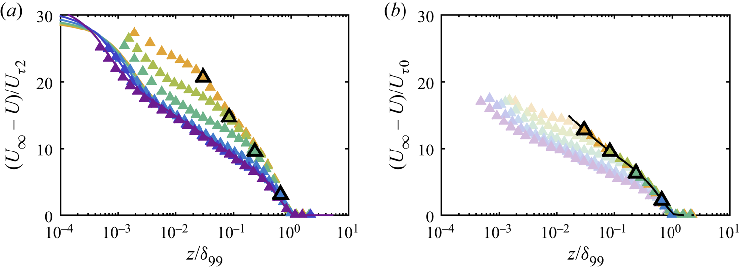
The mean velocity deficit profiles normalised by the friction velocity  $U_{\tau 2}$ obtained locally at the wall are shown in figure 14(a). The corresponding smooth-wall composite profiles at matched
 $Re_{\tau }$ are again shown by coloured lines. A collapse on the smooth-wall reference is observed in the outer layer only at the most downstream locations (at
 $\hat {x}/\delta _0 = 39.4$ and 112, as shown by the dark blue and violet symbols) where the flow has completely recovered to an equilibrium state with the smooth-wall condition. The deficit profiles closer to the step change, however, are above the reference profile, and they gradually relax back to the reference as the fetch increases. The lack of collapse in the inner-normalised velocity deficit suggests an alternative velocity scale in the outer layer above the IBL. We assume the outer-layer velocity scale
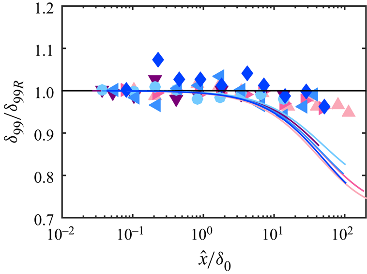
 $U_{\tau ,{out}} = U_{\tau 0}$ as a constant, and present the velocity deficit profiles normalised by this velocity scale in figure 14(b). Under this scaling, the velocity deficit profiles above the IBL collapse reasonably well on the rough-wall reference, which confirms that the flow beyond the IBL scales on the upstream characteristic scales. More details on the evolution of the outer layer can be found in the Appendix A. In essence, for the first few boundary layer thicknesses downstream of the roughness transition, the velocity and length scales in the outer layer evolve with increasing
 $\hat {x}/\delta _0$ in a similar fashion as if the roughness transition did not exist and the upstream roughness extended beyond
 $\hat {x}>0$. Note that the rough-wall reference deficit profile is essentially the same as the smooth-wall deficit profile under outer scaling, as demonstrated in figure 9(a). For the two most downstream locations (dark blue and violet symbols),
 $\delta _i$ has reached
 $\delta _{99}$, therefore no collapse with the rough-wall reference is found under outer scaling.
Mean velocity deficit  $U_{\infty }-U$ for case Re07ks16 normalised by (a)
 $U_{\tau 2}$, the local friction velocity obtained on the smooth wall and (b)
 $U_{\tau 0}$, the friction velocity just upstream on the roughness transition over the rough surface. The abscissa is the outer-scaled wall-normal location
 $z/\delta _{99}$. The coloured lines in (a) are reference smooth-wall composite profiles with
 $Re_{\tau }$ matched at each streamwise measuring location, and the solid black line in (b) is the reference rough-wall hotwire profile obtained in the present study, with the datum adjusted to the smooth surface. The shading of the symbols indicates the downstream fetch, with the specific streamwise locations detailed in the caption of figure 13. Data points within the IBL are shown with a lighter tint in (b) to highlight the outer-layer behaviour. Note that in the two most downstream locations (dark blue and violet symbols),
 $\delta _i$ has already reached
 $\delta _{99}$, therefore the entire profile is shown in the lighter tint and no IBL location is marked.

For figure 14(b), the IBL thicknesses (shown by the symbols with thick black outlines), although determined from the streamwise turbulence intensity profiles, approximately coincide with the location where the mean velocity deficit profile deviates from the rough-wall reference. This is also true for other cases in the current study and the figures are not shown here for brevity. This implies that for the range of  $Re_{\tau 0}$ and
 $k_{s0}^{+}$ investigated, the IBL thickness determined from the mean streamwise velocity and the streamwise turbulence intensity profiles are similar. A similar observation has also been reported by Pendergrass & Arya (Reference Pendergrass and Arya1984) in an experimental study of an internal layer formed over a rough-to-rougher transition, as well as in an open-channel direct numerical simulation (DNS) study with a rough-to-smooth transition (Rouhi et al. Reference Rouhi, Chung and Hutchins2019a) where the intersection of two logarithmic laws in the mean velocity profile coincides with the wall-normal location where the turbulence intensity profile deviates from its upstream counterpart.
7. Blending model of the mean velocity profile
In the seminal work of Elliott (Reference Elliott1958), a theoretical model of a turbulent boundary layer adapting to a step change in the surface condition was developed by evolving an assumed mean velocity profile in the streamwise direction using the momentum equation. The flow both within and above the IBL is modelled by a logarithmic law with the friction velocity chosen as  $U_{\tau 2}$ and
 $U_{\tau 0}$, respectively, representing the stress jump that is assumed to occur at the edge of the IBL. As shown by the experimental data in the previous section, the mean velocity profile above the IBL can be approximated by the upstream rough-wall profile with
 $U_{\tau 0}$ as the velocity scale, while it deviates from the corresponding smooth-wall reference above the equilibrium layer. The deviation of the mean velocity profile from a smooth-wall profile in the IBL has also been previously reported (Antonia & Luxton Reference Antonia and Luxton1971; Garratt Reference Garratt1990; Ismail et al. Reference Ismail, Zaki and Durbin2018; Rouhi et al. Reference Rouhi, Chung and Hutchins2019a; Li et al. Reference Li, de Silva, Baidya, Rouhi, Chung, Marusic and Hutchins2019, for example), demonstrating the necessity of improving the classical mean velocity profile model. Here, we develop a semi-empirical model of the mean velocity profile based on the understanding gained using the present experimental data.
7.1. Description of the model
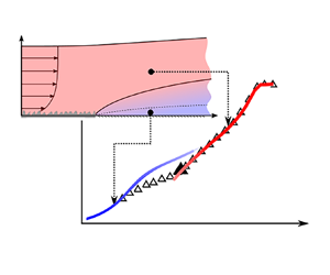
A schematic of the proposed model is illustrated in figure 15. Downstream of a rough-to-smooth change, the flow very close to the wall (within the EL) is expected to have fully adapted to the new wall condition, so it can be approximated by a canonical smooth-wall profile. Above the IBL, the flow is expected to follow the upstream rough-wall scaling and is approximated by a rough-wall profile. We use blue and red colours respectively to represent the completely smooth-wall and rough-wall states of the flow. With an increasing  $z$, we expect the mean flow to gradually transition from the smooth-wall asymptote and be increasingly similar to the rough-wall one, as illustrated by the transition from blue to red in figure 15.
Sketch of a turbulent boundary layer over a rough-to-smooth change, featuring a gradual adjustment of the flow from smooth-wall behaviour (blue) close to the wall to rough-wall behaviour (red) deeper into the flow. The flow is from left to right.

A mathematical description of the qualitative model outlined above is detailed as follows. In the near-wall region where the flow is in full equilibrium with the local smooth wall condition (shown by the blue coloured region in figure 15), the mean velocity distribution satisfies
 \begin{equation} \frac{U(z)}{U_{\tau 2}} = f(z^{+}) \equiv \frac{U_S(z_S)}{U_{\tau S}}, \quad (z\rightarrow 0), \end{equation}
where  $U_{\tau 2}$ is the local friction velocity measured by OFI on the smooth wall,
 $z^{+} = zU_{\tau 2}/\nu$ for the rough-to-smooth profile and
 $z^{+} = z_{S}U_{\tau S}/\nu$ for the smooth-wall reference. The subscript
 $(\cdot )_S$ denotes quantities of the smooth-wall reference. Similarly, above the IBL, the outer-layer similarity is satisfied when normalised by the correct velocity scale, of which
 $U_{\tau 0}$ has been found to be a good approximation when the fetch is not too large (see § 6). The region where the upstream rough-wall scaling is supposed to hold is shown by the red patch in figure 15. The velocity deficit in the outer layer can be expressed as
 \begin{equation} \frac{U_{\infty} - U(z)}{U_{\tau 0}} = g(\eta) \equiv \frac{U_{\infty} - U_{R}(z_R)}{U_{\tau 0}}, \quad (z>\delta_i), \end{equation}
where  $\eta$ is the wall-normal distance normalised by the boundary layer thickness of the corresponding velocity profile, i.e.
 $\eta = z/\delta _{99}$ for the rough-to-smooth profile and
 $\eta = z_{R}/\delta _{0}$ for the rough-wall reference. The subscript
 $(\cdot )_R$ denotes quantities of the rough-wall reference. Note that here the velocity scale is selected as
 $U_{\tau 0}$, the rough-wall friction velocity, for both upstream and downstream mean velocity profiles, as there is no apparent change in the outer-layer velocity scale after the rough-to-smooth change (see § A). Equation (7.2) essentially reduces to
 $U(\eta ) = U_R(\eta )$, therefore a rough-wall velocity profile can be recovered above the IBL (which will include a log and a wake region). As required by (7.2), the applicability of the model relies on an outer-layer similarity above the IBL. For extreme scenarios (such as a very small
 $\delta _0/k$ ratio) where the outer-layer similarity no longer holds, the model would not be expected to work.
In order to combine the two limiting cases described in (7.1) and (7.2), and demonstrate how the recovering profile transitions from the smooth-wall to the rough-wall asymptote as the wall-normal distance increases, we define
 \begin{equation} U^{*+}_{R} = \frac{U_{R}(z_R)}{U_{\tau 2}}, \end{equation}
and plot it against
 \begin{equation} z^{*+}_{R} = \eta\frac{\delta_{99} U_{\tau 2}}{\nu}= \frac{\delta_{99}}{\delta_{0}}\frac{z_R U_{\tau 2}}{\nu} \end{equation}
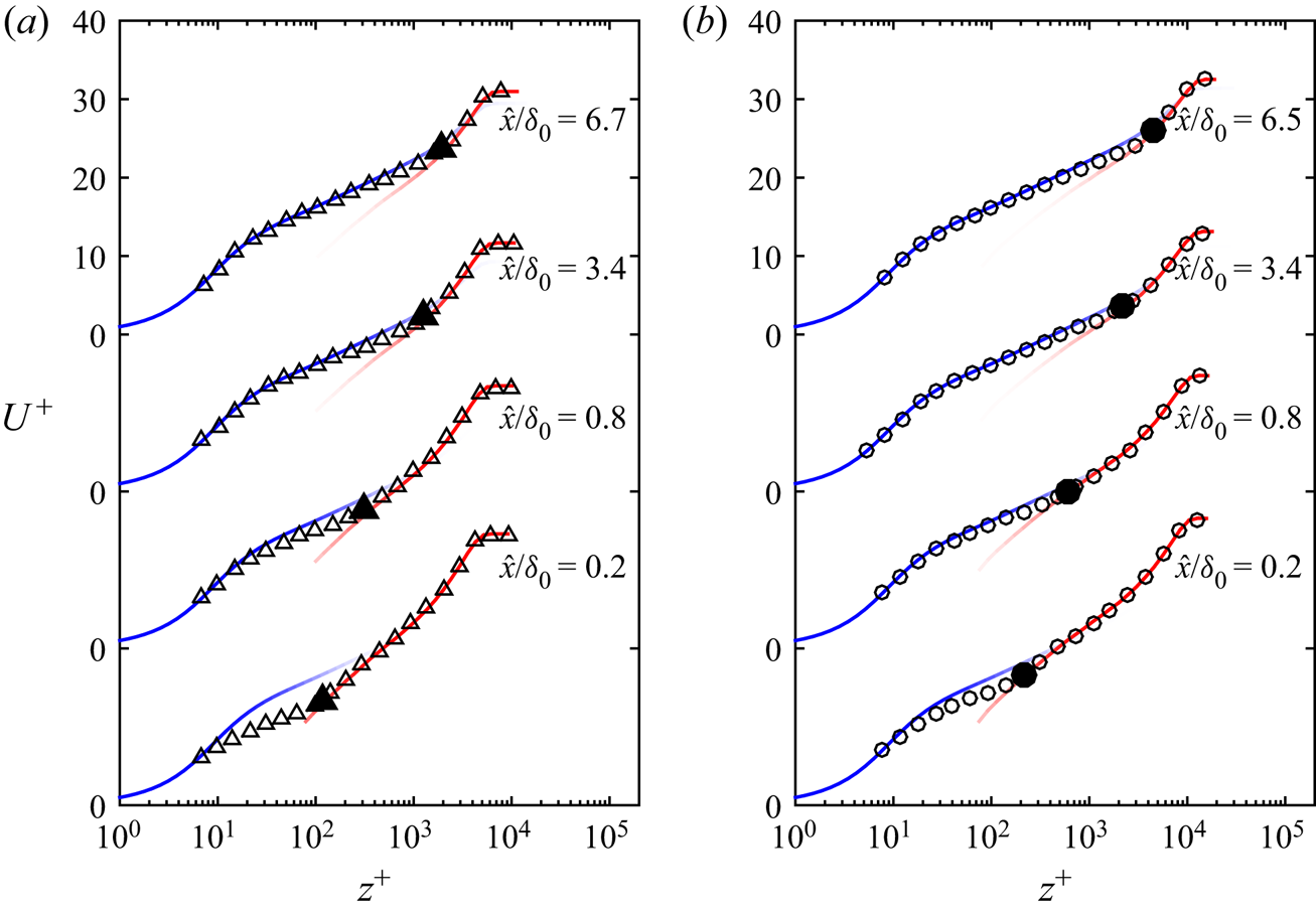
on the inner-normalised mean velocity profiles as shown in figure 16. The  $U^{*+}_{R}$ versus
 $z^{*+}_R$ profile is designed to match the viscous-scaled
 $U^{+}$ versus
 $z^{+}$ profile above the IBL through an assumed outer-layer similarity (7.2), representing the outer layer which is scaled on with the upstream rough-wall velocity scale. The asterisk in the notation is to distinguish it from the conventional inner normalisation where the corresponding friction velocity
 $U_{\tau {R}}$ is used. The smooth-wall reference is chosen as a composite velocity profile (Chauhan et al. Reference Chauhan, Monkewitz and Nagib2009) with the same
 $Re_{\tau }$ as the rough-to-smooth profile, and the rough-wall reference is obtained from the hotwire survey just upstream of the roughness transition at matched flow conditions.
Mean velocity profiles downstream of a rough-to-smooth change normalised by  $U_{\tau 2}$ (empty symbols) compared with the rough-wall and smooth-wall profiles. The blue line is
 $U_S^{+}$ and the red line is
 $U_R^{*+}$. The solid black symbol represents the location of
 $\delta _i$ extracted from the turbulence intensity profile as detailed in § 5. (a) is from case Re07ks16 and (b) is from case Re14ks11.

Without losing generality, we express the recovering mean velocity profile as
 \begin{equation} U^{+} = U_S^{+}E+U_R^{*+}(1-E), \end{equation}
following Krug, Philip & Marusic (Reference Krug, Philip and Marusic2017), who approximated statistics in the wake region of a boundary layer by blending the turbulent and non-turbulent components through a Gaussian distribution of the interface. Here, instead of prescribing a functional form of the blending function  $E(z^{+})$, we aim to obtain that from the measured velocity profiles. At this stage, the only requirement of
 $E(z^{+})$ is that it decreases monotonically from 1 to 0 when
 $z^{+}$ increases from 0 to
 $\delta _{i}^{+}$, corresponding to the limiting cases as the flow fully follows the smooth-wall profile in the vicinity of the wall, and it entirely preserves the upstream rough-wall scaling above the IBL. The EL is implicitly modelled in
 $E(z^{+})$, which will be discussed at the end of this section.
The blending function can be derived by restating (7.5) as
 \begin{equation} E = \frac{U^{+}-U_R^{*+}}{U_S^{+}-U_R^{*+}}. \end{equation}
Here  $U_{S}^{+}$ is the equilibrium smooth-wall composite profile,
 $U_R^{+}$ comes from the measured rough-wall profile upstream of the transition and we have measured
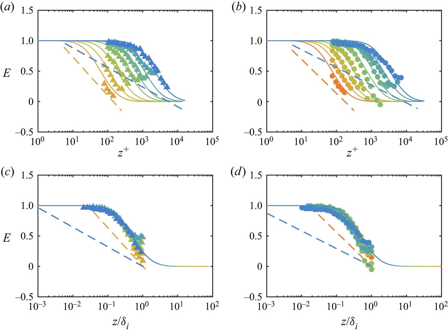
 $U^{+}$ at multiple locations downstream of the transition. The experimentally obtained blending function
 $E(z^{+})$ is shown by the symbols in figure 18 for cases Re07ks16 (a) and Re14ks11 (b) as an example.
The experimentally measured behaviour of  $E$ here appears to be well captured by the cumulative distribution function of a log-normal distribution:
 \begin{equation} E(z^{+};\mu,\sigma) = \frac{1}{2}\left[1-\text{erf}\left(\frac{\ln(z^{+})-\mu}{\sqrt{2\sigma^{2}}}\right)\right], \end{equation}
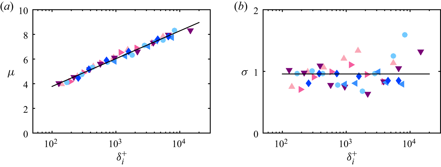
as shown by the solid lines in figure 18. The mean  $\mu$ and standard deviation
 $\sigma$ obtained by fitting (7.7) for all cases are summarised in figure 17. As expected, the averaged location of the flapping interface (captured by
 $\mu$) increases as
 $\delta _i^{+}$ increases with an increasing downstream fetch (figure 17a), while the standard deviation of the flapping interface (
 $\sigma$) appears to remain approximately constant for the entire range. Little
 $Re_{\tau 0}$ or
 $k_{s0}^{+}$ dependence is observed from the data, and a general trend for all cases is found to be
 \begin{equation} \mu = \ln(\delta_i^{+})-0.7,\quad \sigma = 1.0. \end{equation}
The solid coloured lines in figure 18 show the profiles of  $E$ obtained from (7.7) and (7.8a,b), which compare very well with the experimentally determined
 $E$ (shown by the symbols). Subsequently, the recovering mean velocity profile can be obtained by substituting the reconstructed
 $E$ into (7.5). The results are shown by the thick lines with a colour transitioning from blue to red in figure 19, where they are compared with the experimental data (symbols) and the assumed equilibrium profiles (in red and blue). The reconstructed mean velocity profiles are in a better agreement with the experimental data compared with the equilibrium
 $U_S^{+}$ profiles. The improvement is especially notable close to the roughness transition. The modelled velocity profiles of cases Re21ks16 and Re14ks22, which have the largest
 $Re_{\tau 0}$ and
 $k_{s0}^{+}$, respectively, from the current dataset, are also shown in figures 19(c) and 19(d). The model performance remains satisfactory in these extreme cases. The reconstructed mean velocity profile is relatively insensitive to the choice of
 $\sigma$. Varying
 $\sigma$ from 0.7 to 1.5 (which is the range of scatter in figure 17b) leads to less than 3 % change in the reconstructed mean velocity. The uncertainty in
 $U_{\tau 2}$ affects the blending velocity mainly in the near-wall region. In fact, very close to the wall where
 $E\rightarrow 1$, the blending velocity profile is identical to the local smooth-wall reference, therefore the error in the blending velocity profile would simply manifest as scaling the mean velocity with a biased
 $U_{\tau 2}$.
(a) The mean  $\mu$ and (b) standard deviation
 $\sigma$ of all cases obtained by fitting (7.7) to
 $E(z^{+})$ determined experimentally from (7.6). The colour of the symbols indicates
 $Re_{\tau 0}$ or
 $k_{s0}^{+}$ as defined in table 1. Expressions for the solid lines in the figures are given by (7.8a,b).

The blending function  $E$ for (a,c) Re07ks16 and (b,d) Re14ks11. Shading indicates the downstream fetch:
 $\hat {x}$ increases as the colour changes from yellow to blue in each case, as defined in figure 5. The symbols are computed from each hotwire profile from the wall up to the edge of the IBL following (7.6), and the solid lines with corresponding colours represent
 $E$ reconstructed using (7.7) with the parameters given by (7.8a,b). The dashed lines are (7.10) at corresponding streamwise locations, as proposed by Chamorro & Porté-Agel (Reference Chamorro and Porté-Agel2009). (c,d) are the original and reconstructed
 $E$ plotted against
 $z/\delta _i$.

Comparison of the measured (empty symbols) and reconstructed (thick lines with colour transitioning from blue to red) mean velocity profiles downstream of a rough-to-smooth change. The reconstructed velocity profile is obtained using (7.6) and (7.7) with parameters given by (7.8a,b). The blue line is the equilibrium smooth-wall profile  $U_S^{+}$ and the red line is
 $U_R^{*+}$. The solid black symbol represents the location of
 $\delta _i$ extracted from the turbulence intensity profile as detailed in § 5. (a) Re07ks16; (b) Re14ks11; (c) Re21ks16; (d) Re14ks22.

After substituting the fitted expressions (7.8a,b) into (7.7), it is found that the blending function reduces to a self-similar form:
 \begin{equation} E(z/\delta_i) = \frac{1}{2}\left[1-{\rm erf}\left(\frac{\ln(z/\delta_i)+0.7}{\sqrt{2}}\right)\right]. \end{equation}
Here,  $\delta _i$ is the characteristic length scale and
 $E$ is a function of one single variable,
 $z/\delta _i$. The existence of the self-similar behaviour of
 $E$ is further confirmed by plotting the measured
 $E$ against
 $z/\delta _i$. As shown in figure 18(c,d), data from all streamwise locations in both cases collapse on to a single trend that follows (7.9) closely (shown by the solid line). Note that as
 $z/\delta _i$ approaches 1, the denominator
 $U_S^{+}-U_R^{*+}$ in (7.6) becomes increasingly small, which can lead to a higher error and scatter in
 $E$. Nevertheless, the agreement between the measured and reconstructed mean velocity profile is barely affected due to the small difference between
 $U_S^{+}$ and
 $U_R^{*+}$ in this region.
In the existing models in the literature where a wall-normal blending profile is considered, the equilibrium layer thickness  $\delta _e$ is usually prescribed as a fraction of
 $\delta _i$. Abkar & Porté-Agel (Reference Abkar and Porté-Agel2012) used
 $\delta _e/\delta _i = 0.027$ and Ghaisas (Reference Ghaisas2020) found
 $\delta _e/\delta _i = 0.004$ and 0.055 to be optimum for a wind tunnel dataset (Chamorro & Porté-Agel Reference Chamorro and Porté-Agel2009) and a field dataset (Bradley Reference Bradley1968), respectively. These are in good agreement with previous
 $\delta _e$ definitions based on the mean velocity or shear-stress profiles in numerical studies (Shir Reference Shir1972; Rao et al. Reference Rao, Wyngaard and Coté1974; Rouhi et al. Reference Rouhi, Chung and Hutchins2019a). In the context of the blending model,
 $\delta _e$ can also be derived from
 $E$ without any assumption about its dependence on
 $\delta _i$. For instance, by setting a threshold at
 $E=0.99$ (i.e. roughly
 $1\,\%$ difference between
 $U^{+}$ and
 $U_S^{+}$), an equilibrium layer thickness of
 $\delta _e = 0.05\delta _i$ results, and a threshold at
 $E=0.95$ leads to
 $\delta _e = 0.1\delta _i$. Note that the EL thickness determined from either
 $E$ or some other flow statistic profiles is sensitive to the choice of the threshold, especially at a large
 $\hat {x}/\delta _0$ where the recovery is near complete. Therefore, the agreement between these EL thicknesses should only be treated qualitatively.
Chamorro & Porté-Agel (Reference Chamorro and Porté-Agel2009) proposed a similar method to model the non-equilibrium velocity profile with a blending function rearranged to be consistent with the notation in this study as
 \begin{equation} E_c(z^{+}) = 1-\ln\left(\frac{z^{+}}{k_{s0}^{+}\exp(-\kappa A'_{fr})} \frac{U_{\tau R}}{U_{\tau 2}}\right)/\ln\left(\frac{\delta_i^{+}}{k_{s0}^{+}\exp(-\kappa A'_{fr})} \frac{U_{\tau R}}{U_{\tau 2}}\right). \end{equation}
This blending function  $E_c$ at the first and the last streamwise locations is shown in figure 18 by the dashed lines with corresponding colours. Note that the equilibrium smooth-wall and rough-wall profiles were originally modelled by the logarithmic law only, therefore a fair comparison can only be drawn in the expected logarithmic region. A better agreement with the symbols is observed closer to the step change, while the predicted
 $E_c$ falls below the measured data points downstream, resulting in an over-estimation of the contribution from the rough-wall profile during blending.
8. Streamwise turbulence intensity
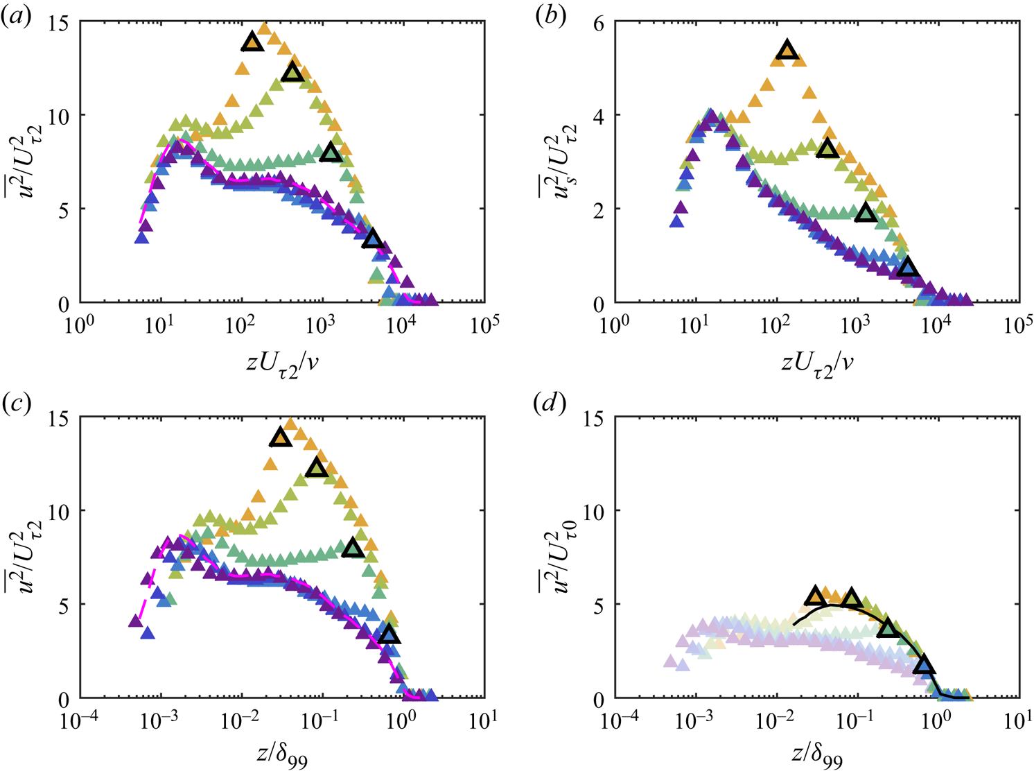
Viscous-scaled streamwise turbulence intensity profiles are shown in figure 20(a) for case Re07ks16. Close to the step change, the peak magnitude of  $\overline {u^{2}}/U_{\tau 2}^{2}$ in the outer layer exceeds the inner peak at
 $z^{+} = 15$ as a result of the highly turbulent rough-wall flow above the IBL, which imposes a footprint onto the near-wall region. The location of the ‘outer peak’ coincides with the edge of the IBL (shown by the bold symbols), and the magnitude of this outer peak decreases with
 $\hat {x}$. A more gradual decreasing trend with
 $\hat {x}$ can also be observed at the inner peak, which eventually reaches the same value as a smooth-wall profile in equilibrium (dashed magenta line). Previously, over a limited range of
 $Re_{\tau 0}$ and
 $k_{s0}^{+}$, we suggested that the collapse in the small-scale energy could be used as a surrogate method of extracting the smooth-wall velocity scale
 $U_{\tau 2}$ in situations where direct measurements in the viscous sublayer are not possible (Li et al. Reference Li, de Silva, Baidya, Rouhi, Chung, Marusic and Hutchins2019). Figure 20(b) shows the small-scale contribution
 $\overline {u^{2}_s}/U_{\tau 2}^{2}$ to the broadband streamwise turbulence intensity. A threshold is selected as
 $1/f^{+} = 200$ (to be detailed in § 9), roughly equivalent to a streamwise wavelength of
 $\lambda _x^{+} = 2000$ at the inner-peak location. Profiles at all streamwise locations collapse well at
 $z^{+}=15$, while the excess energy still presents close to and above
 $\delta _i$ (the IBL location is shown by the symbols with the bold outline). As noted previously, the small-scale contribution recovers almost immediately downstream of a roughness step change (Li et al. Reference Li, de Silva, Baidya, Rouhi, Chung, Marusic and Hutchins2019), and the decreasing trend of the broadband turbulence intensity observed in figure 20(a) at the inner peak is due to the reduction in the footprint of the turbulent motions at larger scales caused presumably by the growth in
 $\delta _i$ with
 $\hat {x}$. This will be discussed more in depth in § 9.
(a) Streamwise turbulence intensity  $\overline {u^{2}}$ profiles and (b) small-scale contribution to the broadband
 $\overline {u^{2}}$ normalised by the local
 $U_{\tau 2}$ and plotted against viscous scaled wall-normal distance. (c,d) are
 $\overline {u^{2}}$ normalised by the local
 $U_{\tau 2}$ and
 $U_{\tau 0}$, respectively, and plotted against outer scaled wall-normal distance. All plots are for case Re07ks16. The symbols with thick black outlines show the location of the IBL (detailed in § 5) in each profile. The shading of the symbols indicates the downstream fetch, with the specific streamwise locations detailed in the caption of figure 13. The dashed magenta line in (a) is a reference smooth-wall hotwire profile with
 $l^{+}=22.7$ measured at
 $Re_{\tau } = 1.0\times 10^{4}$, a Reynolds number matched with the most downstream profile (Marusic et al. Reference Marusic, Chauhan, Kulandaivelu and Hutchins2015). The solid black line in (d) is the reference rough-wall hotwire profile, with
 $z = 0$ shifted downward by
 $|{\rm \Delta} H|$ (the distance between the roughness crest and the smooth wall) to the smooth surface.

The outer ( $z/\delta _{99}$) scaling of the streamwise turbulence intensity profiles with both the local velocity scale (
 $U_{\tau 2}$) and the upstream rough-wall velocity scale (
 $U_{\tau 0}$) is examined in figures 20(c) and 20(d), respectively. These plots can give some indication of the degree of outer layer similarity observed, but a lack of collapse in the near-wall region is enforced by the
 $z/\delta _{99}$ scaling as the abscissa. When normalised by
 $U_{\tau 2}$, the friction velocity obtained locally over the smooth wall,
 $\overline {u^{2}}/U_{\tau 2}^{2}$ downstream of the surface transition is much higher than the smooth-wall reference (shown by the dashed magenta line, which has a viscous-scaled hotwire length of
 $l^{+}=22.7$, comparable with the present dataset), as shown in 20(c). Only for the two most downstream locations (
 $\hat {x}/\delta _0 = 39.4$ and 112, shown by the dark blue and violet symbols) does the outer part of the variance profile scaled in this manner show signs of collapsing to the equilibrium smooth-wall reference. This is presumably because at
 $\hat {x}/\delta _0\geq 39.4$,
 $\delta _i$ has grown close to the edge of the boundary layer, and the entire boundary layer has now almost fully recovered to the smooth wall condition, in consistency with the recovery of mean velocity profiles in figure 14. In figure 20(d), outer-layer similarity between the measurements downstream of the step change and the rough-wall reference (shown by the solid black curve) is observed beyond the IBL, when the upstream friction velocity is chosen as the velocity scale. Note that the dashed magenta line in figure 20(c) and the solid black line in figure 20(d) are expected to collapse under Townsend's assumption of outer-layer similarity, as previously demonstrated in figure 9(b). This is similar to observations made in figure 14 for the mean velocity deficit.
Finally, the effects of  $Re_{\tau 0}$ and
 $k_{s0}^{+}$ on the strength of outer-layer structures are examined by plotting the inner-scaled variance profiles of Group-Re and Group-ks cases at
 $\hat {x}/\delta _0\approx 0.4$ in figures 21(a) and 21(b). Note that the difference in
 $Re_{\tau }$ between Group-ks cases is due to the variation in
 $U_{\tau 2}/U_{\tau 0}$, the ratio of friction velocities across the step change. The variance becomes higher with the increase of
 $Re_{\tau 0}$ and
 $k_{s0}^{+}$. However, within the parameter range in this study, the dependence of the inner-scaled variance on
 $Re_{\tau 0}$ is much less than that on
 $k_{s0}^{+}$. This observation will be revisited in the context of energy spectra in the following section. A collapse in the outer layer is observed in figures 21(c) and 21(d), on the other hand, when the outer length scale
 $\delta _{99}$ and the rough-wall friction velocity
 $U_{\tau 0}$ are used to normalise the profiles, indicating that the outer part of the recovering boundary layer continues to obey outer-layer similarity based on upstream (rough-wall) conditions.
Streamwise turbulence intensity  $\overline {u^{2}}$ at
 $\hat {x}/\delta _0\approx 0.4$ for (a,c) Group-Re and (b,d) Group-ks cases. The top row is normalised by local
 $U_{\tau 2}$ (inner scaling) and the bottom row is normalised by the rough-wall
 $U_{\tau 0}$ and boundary layer thickness
 $\delta _{99}$ (outer scaling). The solid lines are the smooth-wall reference (Marusic et al. Reference Marusic, Chauhan, Kulandaivelu and Hutchins2015; Squire et al. Reference Squire, Morrill-Winter, Hutchins, Schultz, Klewicki and Marusic2016) interpolated to
 $Re_{\tau }$ matched to the corresponding rough-to-smooth profile. The colour of the symbols and lines indicates
 $Re_{\tau 0}$ and
 $k_{s0}^{+}$ in (a,c) and (b,d), respectively, as defined in table 1.

9. Premultiplied energy spectrum
Here, we examine the effect of  $Re_{\tau 0}$ and
 $k_{s0}^{+}$ on the turbulent energy distribution at various wavelengths (i.e. the premultiplied energy spectrum) of flows downstream of the rough-to-smooth transition, especially in light of the large-scale influence in the near-wall region noted in § 8 and by Li et al. (Reference Li, de Silva, Baidya, Rouhi, Chung, Marusic and Hutchins2019).
The premultiplied energy spectrum  $\omega \phi _{uu}/U^{2}_{\tau 2}$ of case Re07ks16 is shown in figure 22, where
 $\omega = 2{\rm \pi} f$ is the angular frequency,
 $f$ is the frequency (corresponding to the wavenumber in the spatial domain),
 $\phi _{uu}$ is the energy spectrum of the streamwise velocity fluctuation (
 $\int _0^{\infty } \phi _{uu}\,\mathrm {d} \omega = \overline {u^{2}}$) and
 $U_{\tau 2}$ is the friction velocity measured from the OFI experiments. The spectrograms are computed from hotwire time-series data. Since the flow is heterogeneous in
 $x$, we refrain from converting the spectrum from the temporal to the spatial domain, which also side-steps uncertainties in convection velocity for rough-wall flows (Squire et al. Reference Squire, Hutchins, Morrill-Winter, Schultz, Klewicki and Marusic2017). The coloured contours are the current rough-to-smooth data, and the white contour lines are interpolated from a reference smooth-wall experimental dataset (Marusic et al. Reference Marusic, Chauhan, Kulandaivelu and Hutchins2015; Squire et al. Reference Squire, Morrill-Winter, Hutchins, Schultz, Klewicki and Marusic2016) at matched
 $Re_{\tau }$, which ensures that the energy diminishes to zero at the same wall-normal height in viscous units in both the rough-to-smooth case and the smooth-wall reference (matched
 $\delta _{99}^{+}$). The coloured contour quite closely follows the white contour lines in the near-wall, high-frequency region of the spectrum, while the difference becomes more noticeable at lower frequencies and with increasing distance away from the wall. Figure 23 shows the difference between the rough-to-smooth spectrum and the reference smooth-wall spectrum, defined as
 \begin{equation} {\rm \Delta} (\omega\phi_{uu}/U_{\tau 2}^{2}) \equiv (\omega\phi_{uu}/U_{\tau 2}^{2})_{R\rightarrow S} - (\omega\phi_{uu}/U_\tau^{2})_{S} \end{equation}
for the downstream locations from  $\hat {x}/\delta _0 = 0.2$ (figure 23a) to 78.7 (figure 23f). Similar to the previous observation (Ismail et al. Reference Ismail, Zaki and Durbin2018; Li et al. Reference Li, de Silva, Baidya, Rouhi, Chung, Marusic and Hutchins2019), the good agreement in the near-wall, small-scale energy spectrum between the rough-to-smooth case and the smooth-wall reference persists at higher
 $Re_{\tau }$ values in the present study. We will refer to this near-wall, high-frequency region where
 ${\rm \Delta} (\omega \phi _{uu}/U_{\tau 2}^{2})$ has reached 0 as ‘the fully-recovered region’. Structures residing above the IBL, which scale on the rough-wall friction velocity
 $U_{\tau 0}$, are over-energised compared with the smaller local
 $U_{\tau 2}$ (the IBL location is marked by the vertical black dashed line in figures 22 and 23). As depicted in figure 23(a–c), these structures leave a ‘footprint’ of excess energy at
 $1/f^{+}\sim O(10^{3})$ in the near-wall region, while the energy distribution at smaller scales is only slightly modified.
Viscous-scaled premultiplied energy spectrum  $\omega \phi _{uu}/U^{2}_{\tau 2}$ as a function of increasing fetch
 $\hat {x}/\delta _0$ from the rough-to-smooth transition. From (a) to (f),
 $\hat {x}/\delta _0 = 0.2,0.8,3.4,15.7,39.4$ and 78.7. The colour contours correspond to the rough-to-smooth case Re07ks16, and the white contour lines are interpolated from a reference smooth-wall experimental dataset to matched
 $Re_{\tau }$. Contour levels are chosen at
 $\omega \phi _{uu}/U^{2}_{\tau 2} = 0$ to 2 with an increment of 0.25. The vertical black dashed line represents the location of
 $\delta _i$. The black plus is at
 $z^{+}=15$ and
 $1/f^{+}=95$ (equivalent to
 $\lambda _x^{+}\approx 1000$). The thick grey dot–dashed lines represent
 $1/f^{+}_{\eta }$, the Kolmogorov time scale. The blue box in (c) is at
 $5<1/f^{+}<90$ and
 $10< z^{+}<30$, showing the region where the spectrum fit is performed.

The difference between the viscous-scaled premultiplied spectrum of Re07ks16 and the smooth-wall reference (matched  $Re_{\tau }$) at streamwise locations corresponding to figure 22. The four black contour lines indicate
 ${\rm \Delta} (\omega \phi _{uu}/U^{2}_{\tau 2}) = 0.25$, 0.5, 0.75 and 1. The vertical dashed black line represents the location of
 $\delta _i$ and the horizontal green dashed line is at
 $1/f^{+} = 2\times 10^{3}$. The black plus is at
 $z^{+}=15$ and
 $1/f^{+}=95$ (equivalent to
 $\lambda _x^{+}\approx 1000$). The thick grey dot–dashed lines represent
 $1/f^{+}_{\eta }$, the Kolmogorov time scale. The blue box in (c) is at
 $5<1/f^{+}<90$ and
 $10< z^{+}<30$, showing the region where the spectrum fit is performed. The blue line is the difference in
 $\phi _{uu}/U_{\tau 2}^{2}$ integrated across all wavelengths.

The fully-recovered region encapsulates turbulence scales from those associated with the near-wall cycle (as marked by the plus symbol in figure 22a) down to the dissipation scales, which can be characterised by the Kolmogorov time scale (Tennekes & Lumley Reference Tennekes and Lumley1972; Pope Reference Pope2000):
 \begin{equation} 1/f^{+}_{\eta} = (\nu/\epsilon)^{1/2}, \end{equation}
where the dissipation rate  $\epsilon$ is estimated from the streamwise energy spectrum as
 \begin{equation} \epsilon = 15\nu\int_0^{\infty}\frac{\omega^{2}}{U^{2}}\phi_{uu}\,\mathrm{d}\frac{\omega}{U}. \end{equation}
The  $1/f^{+}_{\eta }$ is shown in figures 22 and 23 by the thick grey dot–dashed line. The wall-normal extent of the fully-recovered region is initially limited to the buffer region (
 $10< z^{+}<30$) at
 $\hat {x}/\delta _0=0.2$, and gradually expands further away from the wall with the growth of the IBL.
Most previous laboratory measurements only cover a downstream fetch of approximately  $20 \delta _0$ or less, where usually, the flow still has not reached a full recovery to the new wall condition. In the present study, we are able to measure up to
 $120\delta _0$ for case Re07ks16, which enables us to study the recovery of the flow in the far field. A complete recovery of the energy spectrum is achieved at
 $\hat {x}/\delta _0 = 78.7$, as shown in figures 22(f) and 23(f), from which we can estimate that a complete recovery of the energy spectrum can be expected somewhere in the range from
 $39.4\delta _0$ to
 $78.7\delta _0$ downstream of the roughness transition. We lack an intermediate measurement between these locations due to the logarithmic spacing of the streamwise measurement stations. We further examine whether the recovery length remains the same in other cases with different
 $Re_{\tau 0}$ or
 $k_{s0}^{+}$ by compiling the excess energy spectrum contours at several representative streamwise locations into one figure (figure 24), with the
 $x$-coordinate of the centre of each panel as the measurement location. At
 $\hat {x}/\delta _0\approx 15$, all cases have very similar contours of excess energy. The measurement locations become sparse downstream of this point, and there are no measurements beyond this location for Re21ks16 and Re14ks11, the two cases with the longest sandpaper patch. Some excess energy remaining close to the edge of the boundary layer can be observed in Re10ks16, Re14ks22 and Re14ks16 at
 $\hat {x}/\delta _0\approx 40$ (vertical dotted line), while a complete recovery with no distinguishable excess energy is first observed at
 $\hat {x}/\delta _0\approx 80$ (vertical dashed line) in Re07ks16. In summary, from the limited range of
 $Re_{\tau 0}$ and
 $k_{s0}^{+}$ investigated here, no discernible dependence on
 $Re_{\tau 0}$ or
 $k_{s0}^{+}$ in the recovery trends of the excess energy spectrum can be concluded.
The excess energy spectrum of all six cases at various representative streamwise locations. The  $x$-coordinate of the centre of each plot represents the streamwise location where the measurement was obtained. The colour bar is the same as in figure 25. The vertical dotted and dashed lines are at
 $\hat {x}/\delta _0 = 40$ and 80, respectively.

Regardless, the noteworthy feature from these spectra is that it takes a longer fetch downstream for the energy spectrum to relax completely to the smooth-wall state than for the IBL to outgrow the original boundary layer, which is approximately  $26.5\delta _0$ as predicted by extrapolating the power-law fit (5.1). Comparing figures 10 and 23, it appears that, within experimental uncertainty,
 $C_f$ achieves a complete recovery from the roughness transition in a shorter fetch (
 $20\delta _0$) compared with the energy spectrum (
 $40\delta _0$–
 $80\delta _0$). Qualitatively similar observations have been reported by Rouhi et al. (Reference Rouhi, Chung and Hutchins2019a), Ismail et al. (Reference Ismail, Zaki and Durbin2018) and Sridhar (Reference Sridhar2018) in their numerical studies. The streamwise location where
 $C_f$ has reached the complete recovery seems to approximately coincide with the location where the energetic large-scale footprint in the near-wall region vanishes: at
 $\hat {x}/\delta _0 = 15.7$ (figure 23d), this footprint is already becoming very weak for
 $z^{+} < 100$ (marked by the horizontal dashed lines in figure 23).
We further examine the effect of  $Re_{\tau 0}$ and
 $k_{s0}^{+}$ on the recovery behaviour of the energy spectrum utilising both Group-Re and Group-ks. The energy spectra are interpolated to a matched streamwise fetch
 $\hat {x}/\delta _0 = 2$, and summarised in figure 25. We begin by analysing the less complicated Group-ks cases, as shown in figure 25(e–g). Here,
 $\delta _i$ is almost linearly proportional to
 $\hat {x}$ according to (5.1), which implies that both
 $\delta _i U_{\tau 0}/\nu$ and
 $\delta _i/{\delta _{99}}$ are also approximately matched in these Group-ks cases at the matched streamwise location. The excess energy above the IBL is centred around the same location in the frequency domain (similar
 $1/f^{+}$ values), leaving a footprint in the near-wall region as marked by the dashed green lines at
 $1/f^{+} = 2000$. In this study, a higher
 $k_{s0}^{+}$ leads to a higher
 $U_{\tau 0}$ to local
 $U_{\tau 2}$ ratio, so the
 $U_{\tau 0}$-scaled rough-wall structures in the outer layer are more energetic compared with the
 $U_{\tau 2}$-scaled small-scale energy near the wall. Therefore, it is expected that under
 $U_{\tau 2}$ scaling the magnitude of both the outer large-scale motions and their footprints increases with increasing
 $k_{s0}^{+}$, as evidenced by the increasing intensity at a wall-normal location fixed in viscous units (marked by the grey line at
 $z^{+} = 100$) from (e) to (g).
The difference between the viscous-scaled premultiplied spectrum and the smooth-wall reference (matched  $Re_{\tau }$) at
 $\hat {x}/\delta _0=2.0$. (a–d) and (e–g) are Group-Re and Group-ks cases, respectively. The
 $Re_{\tau 0}$ increases from left to right in the first two rows, and
 $k_{s0}^{+}$ increases from left to right in the last row. In each plot, the four black contour lines indicate
 ${\rm \Delta} (\omega \phi _{uu}/U^{2}_{\tau 2}) = 0.25$, 0.5, 0.75 and 1. The vertical dashed black line represents the location of
 $\delta _i$. The vertical grey dotted line shows
 $z^{+} = 100$. The horizontal green dashed line is at
 $1/f^{+} = 2\times 10^{3}$, which serves as a reference of the large-scale footprint locations. The blue curve is the difference in
 $\phi _{uu}/U_{\tau 2}^{2}$ integrated across all wavelengths.

For Group-Re cases at matched  $\hat {x}/\delta _0 = 2$ (figure 25a–d), an increase in
 $\delta _i^{+}$ is expected with an increasing
 $Re_{\tau 0}$, although
 $\delta _i/\delta _{99}$ remains almost constant. With a near constant friction velocity ratio
 $U_{\tau 0}/U_{\tau 2}$, this leads to an almost constant excess energy level in the outer large-scale motions, as evidenced by figure 25(a–d) and also supported by the outer-layer similarity hypothesis above the IBL. As
 $Re_{\tau 0}$ increases, the near-wall footprint is observed to shift to a larger
 $1/f^{+}$ from (a) to (d), while its magnitude decreases slightly. We speculate that the footprinting effect felt in the near-wall region is limited by the increased spatial separation as the large-scale motions are farther away from the wall in viscous units at a greater
 $Re_{\tau 0}$.
To conclude from these observations, the viscous-scaled time period  $1/f^{+}$ of the near-wall footprint from the over-energised large-scale motions increases with
 $Re_{\tau 0}$ while it is little affected by
 $k_{s0}^{+}$. The excess energy in the footprint is found to increase when the large-scale structures in the outer layer are more energised (due to high
 $k_{s0}^{+}$) or closer to the wall in viscous units (due to lower
 $\delta _i^{+}$ which occurs for lower
 $Re_{\tau 0}$ at fixed
 $\hat {x}/\delta _0$).
9.1. Estimating  $U_{\tau 2}$ from the premultiplied energy spectrum

Based on the observation that the energy distribution at the high-frequency end in the near-wall region recovers to the smooth-wall equilibrium state faster than the lower frequencies, Li et al. (Reference Li, de Silva, Baidya, Rouhi, Chung, Marusic and Hutchins2019) previously suggested an alternative method to extract  $U_{\tau 2}$ from the premultiplied energy spectrum when a direct wall-shear stress measurement, such as OFI, is not available. The surrogate method was tested on only one set of data at
 $Re_{\tau 0}=4100$. Here we further examine the validity of this method over a wider range of
 $Re_{\tau 0}$ and
 $k_{s0}^{+}$.
We first provide a brief summary of the method described previously. A rectangular region in the spectrogram plot bounded by the limits  $10< z^{+}<30$ and
 $5<1/f^{+}<90$ is chosen, and the difference between the viscous scaled energy spectra for the rough-to-smooth and the reference smooth cases
 ${\rm \Delta} (\omega \phi _{uu}/U_{\tau 2}^{2})$ is then minimised across this region by varying
 $U_{\tau 2}$. Li et al. (Reference Li, de Silva, Baidya, Rouhi, Chung, Marusic and Hutchins2019) compared the error in the estimation of the spectrum fit method with that from a buffer-region fit of the mean velocity profile, representing conventional methods that assume a canonical or equilibrium mean velocity profile. The proposed spectrum-based technique exhibited much better performance, especially immediately downstream of the roughness transition. Li et al. (Reference Li, de Silva, Baidya, Rouhi, Chung, Marusic and Hutchins2019) defined
 $\epsilon$ as the relative error between the skin-friction coefficient determined from a particular indirect technique and the OFI results as
 \begin{equation} \epsilon \equiv \frac{C_{f}|_{M}-C_{f}|_{OFI}}{C_{f}|_{OFI}}\times 100\,\%. \end{equation}
The subscript  $M$ stands for the method, which can be either the spectrum fit or the buffer-region fit. Li et al. (Reference Li, de Silva, Baidya, Rouhi, Chung, Marusic and Hutchins2019) found that the error of the spectrum fit falls between
 ${\pm }10\,\%$ at all streamwise locations, while an underestimation of over
 $25\,\%$ is observed for the buffer-region fit close to the roughness transition.
In this study we test the efficacy of the surrogate spectral method of estimating  $U_{\tau 2}$ over a much wider range of
 $Re_{\tau 0}$ in figure 26. As shown in (a,b), which compares Group-Re results, the spectrum fit method retains a good agreement with the reference OFI data for all cases, while the buffer-region fit produces an underestimation close to the roughness transition (as noted by Li et al. Reference Li, de Silva, Baidya, Rouhi, Chung, Marusic and Hutchins2019). The spectrum fit method also exhibits similar performance for Group-ks cases, as shown in (c,d). We have previously reported a minimum fetch of
 $5\delta _0$ after the roughness transition before the buffer-region method can be safely used. An even longer fetch (
 $\hat {x}\gtrsim 8h$) is required for the open-channel DNS dataset (which has a much lower
 $Re_{\tau 0}$). For the cases shown in figure 26(a), the error in the buffer-region fit diminishes in a fetch that is typically smaller than
 $2\delta _0$, and the required fetch for reduced error decreases even further as
 $Re_{\tau 0}$ increases. The results indicate that the minimum fetch scales in viscous units rather than
 $\delta _0$ or
 $h$, hence we present
 $\epsilon$ versus
 $\hat {x} U_{\tau 0}/\nu$ in figure 26(b). The results exhibit a much better collapse for the different Reynolds number cases than in figure 26(a) and we observe that a nominally zero
 $\epsilon$ of the buffer-region fit method is observed at
 $\hat {x}U_{\tau 0}/\nu \gtrsim 1.0\times 10^{4}$. The error in the buffer fit method is also seen to increase with increasing
 $k_{s0}^{+}$ in figure 26(d), because the boundary layer is recovering from a greater change.
The error in the estimated  $C_{f}$ relative to the OFI results,
 $\epsilon$, as defined in (9.4). Open symbols represent a buffer region fit and solid symbols are for the spectrum fit. The shaded band covers
 $-10\,\%$ to
 $10\,\%$ on the vertical axis. The first row is for Group-Re cases, and the second row is for Group-ks cases. The colour of the symbols indicates
 $Re_{\tau 0}$ and
 $k_{s0}^{+}$ in the first and second row, respectively, as defined in table 1. The horizontal axis is the fetch normalised by the outer length scale
 $\delta _0$ in (a,c) and the viscous scale in (b,d).

We may conclude that, for a certain  $k_{s0}^{+}$ (and possibly a certain step height), the minimum fetch required before a buffer-region fit can give good wall-shear stress estimates is approximately constant in upstream viscous units. For the buffer-region fit method to be valid, it essentially requires a full recovery of the mean velocity profile within the buffer layer, i.e. the edge of the equilibrium layer should exceed the upper limit of the fitting region. As the upper limit of the buffer region is usually fixed in viscous units, it is expected that the minimum fetch for the equilibrium layer to reach such a height will also be a constant when scaled by viscous units. In fact, the recovery length of the buffer-region fit method can be estimated from the blending function as discussed in § 7. Using the rough approximation
 $\delta _i=0.1\hat {x}$ and a threshold of
 $E=0.95$, the viscous-scaled fetch required for
 $\delta _e^{+}$ to reach the upper limit of the buffer region (i.e. 100 wall units) is found to be
 $\hat {x}U_{\tau 0}/\nu \approx 1.0\times 10^{4}$. Consequently, we can also speculate that a log-region fit to estimate
 $U_{\tau 2}$ (classic Clauser) would require that the equilibrium layer should reach
 $0.15\delta _{99}$, and hence would require a much longer fetch that would scale in
 $\delta _0$.
10. Conclusions
In this study, we present an experimental dataset documenting the evolution of a turbulent boundary layer downstream of a rough-to-smooth surface transition. To redress previously reported uncertainties with  $C_f$ recovery, the skin friction downstream of the transition is measured directly using the OFI technique. In an attempt to unpack the effects of
 $k_{s0}^{+}$ and
 $Re_{\tau 0}$ (which often both vary between studies), the experimental cases are classified into two groups based on their flow conditions. For all Group-Re cases, a nominally constant
 $k_{s0}^{+}\approx 160$ is achieved with
 $Re_{\tau 0}$ ranging from 7100 to 21 000, while a nominally constant
 $Re_{\tau 0}\approx 14\,000$ is achieved for all Group-ks cases with
 $k_{s0}^{+}$ ranging from 111 to 228. Our main findings are summarised as below.
(i) The recovery of
$C_f$ follows a single trend with $\hat {x}/\delta _0$ when normalised by $C_{fe}$ (the skin-friction coefficient expected at the same Reynolds number using the smooth-wall relationship), showing little $Re_{\tau 0}$ or $k_{s0}^{+}$ dependence (figure 10).(ii) A method to extract
$\delta _i$, the IBL height, from the turbulence intensity profile is described. The $\delta _i$ values obtained using this method are compared with the results following the definition of Antonia & Luxton (Reference Antonia and Luxton1971) (which is a commonly used method in the literature), and we show that the present definition leads to a slightly higher $\delta _i$ as it tends to pick up the upper limit of the IBL. The $\delta _i$ computed using both definitions follows a power-law growth trend with increasing development downstream of the transition with an exponent close to 0.8. Little $Re_{\tau 0}$ or $k_{s0}^{+}$ dependence is observed in $\delta _i$, and $\delta _i$ is expected to outgrow the local $\delta _{99}$ at $\hat {x} = 26.5\delta _0$ according to the power law (figure 12).(iii) The mean velocity profile downstream of a rough-to-smooth change is found to undershoot the canonical smooth-wall profile, and it can be modelled by blending the corresponding rough-wall and smooth-wall profiles through a blending function
$E(z)$. This function $E(z)$ can be approximated by an error function with empirically determined parameters, and when $\delta _i$ is selected as the length scale, it also exhibits self-similarity with no dependence on $Re_{\tau 0}$ or $k_{s0}^{+}$ observed within the range of parameters investigated (figure 18).(iv) A complete recovery of the energy spectrum occurs within a fetch between 40 and
$80\delta _0$ for case Re07ks16, longer than the fetch required for $\delta _i$ to outgrow $\delta _{99}$ as predicted by the power-law relation. The recovery length has shown little dependence on $Re_{\tau 0}$ or $k_{s0}^{+}$ when normalised by $\delta _0$ (figure 23).(v) The over-energised inner peak observed in the streamwise turbulence intensity profiles is found to be contributed by the large-scale motion footprints in the near-wall region. The viscous-scaled time period (
$1/f^{+}$) of these footprints increases with $Re_{\tau 0}$ while it is little affected by $k_{s0}^{+}$. The excess energy in the footprint is found to increase when the large-scale structures in the outer layer are more energised (due to high $k_{s0}^{+}$) or closer to the wall in viscous units (due to lower $\delta _i^{+}$ which occurs for lower $Re_{\tau 0}$ at fixed $\hat {x}/\delta _0$) (figure 25).(vi) The spectrum fit method to extract local friction velocity proposed by Li et al. (Reference Li, de Silva, Baidya, Rouhi, Chung, Marusic and Hutchins2019) exhibits a good performance over a wide range of
$Re_{\tau 0}$. For an equilibrium layer with a growth rate similar to the present study, the error in the estimation from a buffer-region fit of the mean velocity profile is considered to diminish after $\hat {x}U_{\tau 0}/\nu \gtrsim 1.0\times 10^{4}$ (figure 26).(vii) The length and velocity scales in the outer layer remain relatively unchanged right after the rough-to-smooth change. Farther downstream, both
$C_{f,\textit{out}}$ and $\delta _{99}$ begin to slowly adapt to the smooth-wall state, presumably as the over-energised large-scale structures in the outer layer decay and are replaced by events that reflect the new surface condition. A noticeable deviation from the rough-wall trend only appears after approximately $10\delta _0$ downstream of the transition (figures 27 and 29).


The boundary layer thickness,  $\delta _{99}$, determined from the measured mean velocity profiles downstream of the rough-to-smooth normalised by
 $\delta _{99R}$, the boundary layer thickness for a homogeneously rough surface. The solid black line is at
 $\delta _{99}/\delta _{99R} = 1$. Reference curves are included for comparison, which are predicted using the von Kármán momentum integral equation assuming that the boundary layer immediately adjusts to a smooth-wall profile with matched
 $\delta _{99}$ right after the rough-to-smooth transition and shown by solid line with a colour corresponding to each case.

To conclude, downstream of a rough-to-smooth change, many statistics of the recovering flow, such as  $C_f$,
 $\delta _i$ and
 $E(z)$, are little affected by
 $Re_{\tau 0}$ and
 $k_{s0}^{+}$ when scaled properly. This observation is meaningful in the application of high-Reynolds-number atmospheric or industrial flows beyond laboratory ranges. In the current study, the range of
 $k_{s0}^{+}$ is limited compared with other studies such as that of Hanson & Ganapathisubramani (Reference Hanson and Ganapathisubramani2016). Hence, a wider range of
 $k_{s0}^{+}$ values needs to be investigated in future works in search of potential
 $k_{s0}^{+}$ effects.
Funding
This research was partially supported under the Australian Research Council's Discovery Projects funding scheme (project DP160103619).
Declaration of interests
The authors report no conflict of interest.
Appendix A. Evolution of the outer layer
Traditionally, studies on the flow downstream of a roughness transition have tended to focus on the thickness of the developing IBL and the local friction velocity. The length and velocity scales in the outer layer are usually assumed to remain constant and the evolution of the outer layer in the streamwise direction is often neglected (for example Elliott Reference Elliott1958; Panofsky & Townsend Reference Panofsky and Townsend1964; Chamorro & Porté-Agel Reference Chamorro and Porté-Agel2009). In addition, the mean velocity profile in the outer layer is often characterised by a logarithmic law only and the boundary layer thickness  $\delta _{99}$ often does not feature in the modelled or assumed profiles. These assumptions may be adequate in a short fetch downstream of the transition, where the recovery of the flow is rapid and the Reynolds number does not change substantially. However, even in a turbulent boundary layer developing on a homogeneous surface in a zero-pressure gradient, the streamwise evolution of the flow leads to an increase in the boundary layer thickness and a decrease in the friction velocity with increasing
 $x$. The decrease in the outer-layer friction velocity scale
 $U_{\tau ,{out}}$ has been shown to be enhanced following a rough-to-smooth change (Hanson & Ganapathisubramani Reference Hanson and Ganapathisubramani2016). Here, utilising the current experimental dataset, the far-field evolution of
 $\delta _{99}$ and
 $U_{\tau ,{out}}$ is investigated and compared with that of a homogeneous rough-wall or smooth-wall boundary layer.
A.1. Boundary layer thickness
The growth of the boundary layer thickness  $\delta _{99}(\hat {x})$ downstream of the rough-to-smooth transition is compared with
 $\delta _{99R}$, the thickness that a boundary layer developing on a homogeneously rough surface would have. Here,
 $\delta _{99R}$ is computed by integrating the von Kármán momentum integral equation (Monty et al. Reference Monty, Dogan, Hanson, Scardino, Ganapathisubramani and Hutchins2016) in the streamwise direction. The ratio
 $\delta _{99}(\hat {x})/\delta _{99R}(\hat {x})$ for all cases is presented in figure 27. This ratio is very close to 1 (shown by the solid black line) in the vicinity of the roughness transition, which suggests that the growth rate of a rough-wall boundary layer thickness is initially sustained after the transition. Farther downstream, a consistent deviation from unity is observed, especially in case Re07ks16 which has the longest fetch on the downstream smooth wall. A
 $\delta _{99}/\delta _{99R}$ ratio smaller than 1 indicates that the boundary layer thickness after a rough-to-smooth change is smaller than its rough-wall counterpart at the same fetch. A reference
 $\delta _{99}/\delta _{99R}$ curve can be further provided assuming that the entire boundary layer immediately adjusts to a smooth-wall mean velocity profile with matched
 $\delta _{99}$ right after the rough-to-smooth transition, which is also computed following the same method of Monty et al. (Reference Monty, Dogan, Hanson, Scardino, Ganapathisubramani and Hutchins2016) and shown by coloured solid lines in figure 27. This is referred to as the ‘immediate-change reference’ in the following text. All data points of the present cases are above the immediate-change reference lines.
A.2. Velocity scale
Elliott's (Reference Elliott1958) model of the developing flow downstream of a rough-to-smooth transition assumes that above the IBL,  $U_{\tau 0}$ (the friction velocity over the upstream rough surface) is the correct velocity scale, which implies that the over-energised outer turbulence continues to reflect the upstream roughness velocity scale, even far downstream of the transition, and does not decay or relax in the downstream.
Hanson & Ganapathisubramani (Reference Hanson and Ganapathisubramani2016) calculated the friction velocity  $U_{\tau ,{out}}$ required to force the collapse of the mean velocity deficit on a smooth-wall reference above the internal layer. They reported that all
 $C_{f,{out}}(\equiv 2U_{\tau ,{out}}^{2}/U_{\infty }^{2})$ values are less than
 $C_{f0}$, the skin-friction coefficient on the upstream rough surface, and it decays in the streamwise direction and approaches (though has not reached) the local smooth wall
 $C_f$ at the last measuring location at
 $\hat {x}/\delta _0 \approx 20$. Data from their original figure 19(a) are reproduced here in figure 28(b) for comparison. The
 $C_{f,{out}}$ for case Re07ks16 computed following the same procedure as of Hanson & Ganapathisubramani (Reference Hanson and Ganapathisubramani2016) is shown in figure 28(a). Note that similar behaviours are observed in all other cases, and are not shown here for brevity. Two definitions of
 $\delta _i$ are tested: the classic one based on the
 $U$ versus
 $z^{1/2}$ profile originally proposed by Antonia & Luxton (Reference Antonia and Luxton1971) and used by Hanson & Ganapathisubramani (Reference Hanson and Ganapathisubramani2016), and the current definition based on the turbulence intensity profile as detailed in § 5. The resulting
 $C_{f,{out}}$ with
 $\delta _i$ computed from these two definitions are shown in figure 28(a) by empty black and solid pink triangles, respectively. In the present study,
 $\delta _i$ is defined as the upper limit of the (assumed) fluctuating rough/smooth interface, while the definition used by Hanson & Ganapathisubramani (Reference Hanson and Ganapathisubramani2016) appears to be closer to the averaged location of the (assumed) fluctuating interface. As
 $\delta _i$ grows and approaches the local
 $\delta _{99}$, the fitting range of the outer layer diminishes and eventually there are not enough data points to perform the regression, making the
 $C_{f,{out}}$ trend in the limit of large
 $\hat {x}/\delta _0$ unattainable. There is little difference between the two
 $C_{f,{out}}$ results except at the last few downstream locations, where the solid pink triangles (with
 $\delta _i$ defined based on the turbulence intensity profile) are absent due to the vanishing of the fitting range as
 $\delta _i$ approaches
 $\delta _{99}$. With Antonia and Luxton's definition of
 $\delta _i$, a larger portion of the velocity profile which has in fact been affected by the new smooth-wall condition is included in the fit, therefore, a distinct decrease presents in
 $C_{f,{out}}$, qualitatively similar to the near collapse in
 $C_{f,{out}}$ and
 $C_f$ at their most downstream station as reported by Hanson & Ganapathisubramani (Reference Hanson and Ganapathisubramani2016).
Skin-friction coefficient  $C_f$ obtained within the IBL and above the IBL via curve fitting for (a) case Re07ks16 and (b) case grit adapted from the study by Hanson & Ganapathisubramani (Reference Hanson and Ganapathisubramani2016). Empty pink triangles in both figures are
 $C_f$ measured in the near-wall region, while empty black and filled pink triangles are
 $C_{f,{out}}$ computed assuming an outer-layer similarity in the mean velocity deficit with
 $\delta _i$ estimated following the method of Antonia & Luxton (Reference Antonia and Luxton1971) and the thresholding approach as detailed in § 5, respectively. The black dashed line is
 $C_{fR}$ of a homogeneous rough-wall boundary layer without the change of surface condition at
 $x_0$ computed by integrating the von Kármán momentum integral equation (Monty et al. Reference Monty, Dogan, Hanson, Scardino, Ganapathisubramani and Hutchins2016), and the blue arrow shows the skin-friction coefficient at the reference upstream rough-wall measurement.

The skin-friction coefficient for a homogeneously rough surface (with the same roughness as the upstream surface)  $C_{fR}(\hat {x})$ is also included for comparison in figure 28 (black dashed line), which is computed through the same streamwise evolution as that employed in § A.1 to obtain
 $\delta _{99R}$. (To predict the corresponding
 $C_{fR}(\hat {x})$ for Hanson and Ganapathisubramani's dataset, we use
 $\varPi _j = 0.71$ as reported for their homogeneous smooth-wall boundary layer. Here
 $k_s$ is calculated from the reported viscous-scaled roughness length
 $z_0^{+}$ of the rough surface, and
 $\kappa = 0.41$ and
 $B = 5.0$ are used in the evolution to be consistent with their choice of the constants. The initial condition of the evolution is adjusted such that the resulting
 $C_{fR}(0)$ matches the reported skin-friction coefficient just upstream of the roughness transition.) Just prior to the surface transition, the
 $C_{fR}(0)$ obtained from the measured upstream rough-wall profile is shown by a blue arrow on the logarithmic abscissa. Figure 28 shows that
 $C_{f,{out}}$ closely follows the predicted value for a homogeneously rough surface in the present dataset, while an immediate decrease in
 $C_{f,{out}}$ compared with its value on the rough wall upstream is reported by Hanson & Ganapathisubramani (Reference Hanson and Ganapathisubramani2016), which can be readily observed in (b). In figure 28(b),
 $C_{f,{out}}$ at the first downstream location is lower than the rough-wall reference
 $C_{fR}(0)$ by
 $22\,\%$. Such a sudden change in the velocity scale in the outer layer challenges the traditional view that the effect of the new surface condition gradually modifies the interior of the flow through the growth of the IBL. Future work is required to further verify the existence of this behaviour and to understand the mechanisms behind it. Certainly, for the present measurements (figure 28a), this effect is not observed.
We further examine the change of  $C_{f,{out}}$ with
 $\hat {x}$ for all cases. Figure 29 shows
 $C_{f,{out}}(\hat {x})$ normalised by
 $C_{fR}(\hat {x})$ for all cases. The
 $C_{f,{out}}$ is computed by assuming an outer-layer similarity in the mean velocity deficit and turbulence intensity profiles in (a) and (b), respectively. If the velocity scale (i.e. rough-wall friction velocity) in the outer layer continues to develop as before without being affected by the rough-to-smooth transition, then
 $C_{f,{out}}/C_{fR}$ should equal 1, as shown by the solid black line. Note that the focus here is on the trend of the streamwise evolution of
 $C_{f,{out}}/C_{fR}$ in the streamwise direction rather than to assess how well the skin-friction coefficient predicted using the von Kármán momentum integral equation matches the measurement on the rough wall. For this reason we divide all the downstream points by
 $C_{f,{out}}/C_{fR}$ at the first downstream measuring station, forcing the points immediately downstream of the transition in figure 29 to 1. This reduces the scatter of the data and facilitates the identification of an overall trend. The correction is usually less than
 $15\,\%$ in (a) and
 $3\,\%$ in (b), presumably indicative of the accuracy with which
 $C_{f,{out}}$ can be determined by the two methods, and it does not show any dependence on
 $Re_{\tau 0}$ or
 $k_{s0}^{+}$.
The  $C_{f,{out}}$ normalised by
 $C_{fR}$, the skin-friction coefficient for a homogeneously rough surface. The
 $C_{f,{out}}$ is calculated by assuming an outer-layer similarity in (a) mean velocity deficit and (b) turbulence intensity profiles. The coloured filled symbols represent cases in the present study, and the black crosses are computed from the dataset of Hanson & Ganapathisubramani (Reference Hanson and Ganapathisubramani2016). The solid black line is
 $C_{f,{out}}/C_{fR} = 1$.

Due to the uncertainty of the measurement and the fitting method,  $C_{f,{out}}$ computed from the mean velocity deficit (figure 29a) exhibits
 ${\pm }10\,\%$ scatter, while a less scattered trend is observed when the streamwise turbulence intensity profile is used (figure 29b). Overall,
 $C_{f,{out}}/C_{fR}$ shows a slightly decreasing trend, and for all cases, it falls below 1 (shown by the solid black line) at
 $\hat {x}/\delta _0\approx 15$, the last streamwise location where
 $C_{f,{out}}$ is attainable. For the homogeneously rough surface,
 $C_{fR}$ decreases in the streamwise direction as the boundary layer grows and the Reynolds number increases. The decreasing trend of the ratio
 $C_{f,{out}}/C_{fR}$ suggests that the velocity scale in the outer layer decreases marginally more aggressively than the Reynolds number trend of
 $C_{fR}$, i.e.
 $C_{f,{out}}/C_{fR}$ decreases slightly faster after a rough-to-smooth change than it would without the roughness transition. The physical interpretation is the production of turbulent energy at the wall decreases after a rough-to-smooth change and, with a reduced supply of turbulent energy, the outer layer cannot sustain a rough-wall friction velocity that is no longer compatible with the new wall condition. Therefore, the velocity scale in the outer layer decreases more aggressively than the Reynolds number trend. The slow decay is presumably indicative of the time scale of the large-scale outer structures through which the boundary layer retains memory of upstream conditions.
Despite the small difference between  $C_{f,{out}}$ and
 $C_{fR}$, this further supports the conclusion in §§ 6 and 8 that the velocity scale in the flow above the IBL is very close to the friction velocity of the rough wall upstream, and may in fact prove to be a reasonable modelling assumption in Elliott's approach.
It should be stressed that the determination of both  $C_{f,{out}}$ and
 $\delta _{99}$ suffer from a degree of uncertainty; however, we still observe a weak trend in both of them where they fall below the corresponding rough-wall value in the far field. The general picture is that when a turbulent boundary layer encounters a rough-to-smooth change, the change is barely felt in the outer layer at first and the flow in the outer layer continues to evolve in the streamwise direction as if the roughness transition was not there. Farther downstream, both
 $C_{f,{out}}$ and
 $\delta _{99}$ begin to slowly adapt to the smooth-wall state, presumably as the over-energised large-scale structures in the outer layer, which retain the memory of the upstream conditions, decay and are replaced by events that reflect the new surface condition. A noticeable deviation from the rough-wall trend only appears after approximately
 $10\delta _0$ downstream of the transition.
Appendix B. Procedure to apply the blending model
Here, we summarise the procedure to generate a velocity profile using the blending model described in § 7. The upstream rough-wall velocity profile, the IBL thickness  $\delta _i$, local friction velocity
 $U_{\tau 2}$ and boundary layer thickness
 $\delta _{99}$ at a certain distance downstream of the rough-to-smooth change are required as inputs to the model. The steps are detailed as follows.
(i) Generate the blending function
$E(z^{+})$ from (7.7) and (7.8a,b).(ii) Generate the smooth-wall limit
$U_S^{+}(z^{+})$, i.e. a composite velocity profile (Chauhan et al. Reference Chauhan, Monkewitz and Nagib2009) with $Re_{\tau } = \delta _{99}U_{\tau 2}/\nu$.(iii) Compute the rough-wall limit
$U_R^{*+}(z_R^{*+})$ following (7.3) and (7.4).(iv) Obtain the final blending velocity profile at the given streamwise location through (7.5).