1. Introduction
Buoyancy-driven turbulent flows occur in many natural phenomena and engineering applications, including astrophysics, earth sciences, inertial confinement fusion and combustion systems. An extensive list of many such examples can be found in the review article by Zhou (Reference Zhou2017a). Often, these flows involve the complex coupling of many physical phenomena such as buoyancy, combustion, multiphase interactions and shocks. Direct numerical simulation (DNS) of turbulent flows is prohibitively expensive and practically impossible for most applications, and flow modelling is necessary to account for the unresolved parts of the flow. To aid the development of such models, various flow physics can be isolated using canonical problems. Such problems afford scientists deeper physical understanding of the flow physics and also function as computationally tractable validation test beds for model development.
The Rayleigh–Taylor instability (Rayleigh Reference Rayleigh1882; Taylor Reference Taylor1950) occurs between fluids of different densities, when the light fluid is accelerated into the heavy by an external pressure gradient. A canonical flow configuration used extensively to study such instabilities is the planar Rayleigh–Taylor (RT) flow configuration. Two fluids of different densities are initially separated by a planar interface in an unstable configuration and accelerated by a constant gravitational force normal to the interface. The RT configuration has been studied extensively, and many of the key contributions are summarized in several review articles. Zhou (Reference Zhou2017a,Reference Zhoub) contains a comprehensive overview of RT-related research, while more focused reviews on theoretical modelling (Abarzhi Reference Abarzhi2010), RT turbulence in the Boussinesq limit (Boffetta & Mazzino Reference Boffetta and Mazzino2017) and experiments (Andrews & Dalziel Reference Andrews and Dalziel2010; Banerjee Reference Banerjee2020) also exist. Finally, Schilling (Reference Schilling2020) summarizes efforts and potential opportunities for integrating simulation, modelling and experiments.
1.1. Rayleigh–Taylor instability
In the canonical RT configuration, a heavy fluid sits atop a light fluid in the presence of a constant acceleration field, such as gravity. The flow is initially stationary, and pure reservoirs of heavy and light miscible fluid are separated by an infinitely thin and flat interface situated at  $x_2=\delta _I$. These initial conditions are
 $$\begin{gather} \rho(t=0,\boldsymbol{x}) = \left\{\begin{array}{@{}ll@{}} \rho_L, & x_2 < \delta_I, \\ \rho_H, & x_2 > \delta_I, \end{array} \right. \end{gather}$$
 $$\begin{gather}\boldsymbol{u}(t=0,\boldsymbol{x}) = 0, \end{gather}$$
where  $\rho$ is the density and
 $\boldsymbol {u}$ the velocity. The subscripts
 $H$ and
 $L$ indicate the properties of the heavy and light fluids, respectively. Gravity acts vertically downwards, i.e.
 $g_i = -g \delta _{2i}$.
In the presence of small perturbations at the interface, RT instabilities develop. Linear stability analysis predicts exponential growth at all wavelengths in the inviscid limit (Rayleigh Reference Rayleigh1882; Taylor Reference Taylor1950), while viscosity (Chandrasekhar Reference Chandrasekhar1955) and diffusivity (Duff, Harlow & Hirt Reference Duff, Harlow and Hirt1962) have been found to inhibit small-scale growth. As perturbations grow, nonlinearities become important and the flow undergoes a transition to turbulence.
1.2. Self-similarity in turbulent Rayleigh–Taylor flows
As the flow transitions to turbulence, it is widely believed that an asymptotic self-similar regime exists. In this regime, Youngs (Reference Youngs1984) observed a quadratic growth of the mixing layer height,  $h \approx \alpha Agt^2$. By applying similarity assumptions to the governing equations, Ristorcelli & Clark (Reference Ristorcelli and Clark2004) derived an equivalent result
 \begin{equation} \dot{h}^2 = 4\alpha A g h, \end{equation}
where  $h(t)$ is a mixing layer height,
 $\dot {h} = {\rm d}h/{\rm d}t$,
 $A = (\rho _H-\rho _L)/(\rho _H+\rho _L)$ is the Atwood number and
 $\alpha$ is a dimensionless growth parameter. Although the relationship
 $\dot {h}^2\propto h$ is valid for any height definition, the specific value of
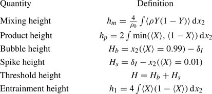
 $\alpha$ depends on the choice of height definition. All height definitions used in this paper are listed in table 1.
Different definitions of the mixing layer height. Here,  $X$ and
 $Y$ are the mole and mass fractions of the heavy fluid;
 $\rho _0= 2\rho _H \rho _L/(\rho _H+\rho _L)$ is a normalization density;
 $\delta _I$ is the initial interface location. All integrals in
 $x_2$ are taken from
 $x_2=-\infty$ to
 $x_2=+\infty$.

Self-similarity in RT flows is typically demonstrated by stationarity in normalized statistics. For example, the growth parameter  $\alpha$ is commonly used as evidence of self-similarity, as are various measures of mixedness (Zhou, Cabot & Thornber Reference Zhou, Cabot and Thornber2016). For planar-averaged quantities that vary along the vertical direction, data from different simulation times should collapse onto each other when normalized suitably. Typically, the vertical coordinate is normalized by the height of the mixing layer
 $h$, and self-similarity has been demonstrated with various height definitions. Velocities can be scaled with
 $\dot {h}$ (e.g. Zhou & Cabot Reference Zhou and Cabot2019) or
 $(gh)^{1/2}$ (e.g. Vladimirova & Chertkov Reference Vladimirova and Chertkov2009). Equivalently, the total kinetic energy of the flow can be scaled by the potential energy loss of the flow (e.g. Cabot & Cook Reference Cabot and Cook2006). These velocity scalings are all consistent, by virtue of (1.3).
This self-similar growth is commonly associated with three conditions that are satisfied by late-time RT flow (Youngs Reference Youngs1984; Cook, Cabot & Miller Reference Cook, Cabot and Miller2004).
(i) In an infinitely large domain, the mixing layer height
 $h(t)$ eventually becomes much larger than any characteristic length scale of the initial interface perturbations $\ell _I$. When $h(t)\gg \ell _I$, the flow loses memory of its initial conditions, and flow structures grow in size solely through the merger of smaller structures (or mode-coupling processes).
(ii) The flow transitions to turbulence, and widening scale separation between the buoyancy-driven large scales and the viscous/diffusive small scales leads to
$h(t) \gg \eta$, where $\eta$ is the Kolmogorov length scale commonly used to characterize the small turbulence scales. An equivalent condition can be stated in terms of the Reynolds number. For RT flow, the mixing layer Reynolds number can be defined as
(1.4)where\begin{equation} Re = \frac{H\dot{H}}{\nu}, \end{equation}$H(t)$ is defined in table 1, $\dot {H} = {\rm d}H/{\rm d}t$ and $\nu$ is the kinematic viscosity. This definition was chosen to be consistent with Cabot & Cook (Reference Cabot and Cook2006), which will be used as a recurring reference for comparison in this paper. For the flow to be turbulent, $Re(t)\gg 1$.(iii) In an infinite three-dimensional domain, when
$h(t) \gg \ell _I,\eta$, the mixing layer evolution is fully characterized by its height and the flow is self-similar. However, in practice, any experiment or simulation must be performed on a domain of a finite size ${\mathcal {L}}$. Obviously, vertical boundaries should be much larger than $h(t)$. Additionally, confinement effects from the lateral domain boundaries also modify the qualitative nature of RT turbulence (Dalziel et al. Reference Dalziel, Patterson, Caulfield and Coomaraswamy2008; Boffetta, De Lillo & Musacchio Reference Boffetta, De Lillo and Musacchio2012a; Boffetta et al. Reference Boffetta, De Lillo, Mazzino and Musacchio2012b). Hence, to approximate RT mixing layer growth in an infinite domain, the third condition for finite-domain RT flows is $h(t)\ll {\mathcal {L}}$.


Summarily, these three conditions can be stated as
 \begin{equation} \ell_I,\eta \ll h(t) \ll {\mathcal{L}}. \end{equation}
The difficulty in satisfying the contradicting requirements of (i) and (iii) is well illustrated by the discrepancies in observed  $\alpha$ values between experiments and simulations (Dimonte et al. Reference Dimonte2004; Boffetta & Mazzino Reference Boffetta and Mazzino2017). Using a bubble height definition, experiments consistently yield
 $\alpha$ values in the range of 0.05–0.08, while simulations produce smaller values of 0.02–0.03. This has been attributed to differences in wavelength content of the initial perturbations. Specifically, Ramaprabhu & Andrews (Reference Ramaprabhu and Andrews2004b) and Mueschke & Schilling (Reference Mueschke and Schilling2009a,Reference Mueschke and Schillingb) simulated RT growth using experimentally measured initial conditions and successfully reproduced larger
 $\alpha$ values comparable to those from experiments. Other numerical studies (Ramaprabhu, Dimonte & Andrews Reference Ramaprabhu, Dimonte and Andrews2005; Banerjee & Andrews Reference Banerjee and Andrews2009; Youngs Reference Youngs2013) have also confirmed that smaller (respectively larger)
 $\alpha$ values are observed when initial perturbations are applied only at the smallest scales (respectively over a wide range of scales). This paper focuses solely on the late-time, infinite-domain limit described by (1.5), also known as the mode-coupling (Ramaprabhu et al. Reference Ramaprabhu, Dimonte and Andrews2005; Youngs Reference Youngs2013) or ‘ideal’ (Zhou Reference Zhou2017a) case. Any subsequent mention of self-similar RT growth in this paper refers specifically to this case.
It is worth clarifying that the typical interpretation of self-similarity in turbulent RT flows does not imply that all quantities are statistically stationary when normalized with a single set of normalization scales. At the large scales, viscosity and diffusivity have no effect, and all large-scale quantities can be normalized by  $A$,
 $g$ and
 $h$. The specific interpretation of self-similarity used in this paper is: (a) all quantities demonstrate statistical stationarity when normalized appropriately; (b) specifically, the large-scale dynamics is buoyancy driven, and the appropriate normalization of the large scales involves length scale
 $h$, and time scale
 $(h/Ag)^{1/2}$.
The relative importance of conditions (i) and (ii) is also an open question. As an RT flow evolves in time, its memory of the initial conditions fades and its Reynolds number increases. Both conditions are consistent with the observation that self-similarity is approached at late times. However, both conditions are intrinsically linked in temporally evolving RT flows and cannot be studied independently. In particular, no minimum threshold Reynolds number has been established for the existence of self-similar RT behaviour, nor is there a framework for assessing how long a given initial condition would take to be sufficiently forgotten.
From a modelling perspective, self-similarity is an assumption utilized by many Reynolds-averaged Navier–Stokes models to reduce the complexity of the RT governing equations (Dimonte & Tipton Reference Dimonte and Tipton2006; Banerjee, Gore & Andrews Reference Banerjee, Gore and Andrews2010a; Morgan & Wickett Reference Morgan and Wickett2015; Schilling Reference Schilling2021). To derive analytical forms of the self-similar fields and calibrate model coefficients, accurate data of high  $Re$ self-similar RT turbulence are required. The challenges associated with such efforts are discussed in Schilling (Reference Schilling2021). Direct numerical simulation has been used to provide modelling insights (Livescu et al. Reference Livescu, Ristorcelli, Gore, Dean, Cabot and Cook2009; Schilling & Mueschke Reference Schilling and Mueschke2010, Reference Schilling and Mueschke2017), but sources of high
 $Re$ self-similar RT data are rare, and it remains questionable if any have reached full self-similarity.
1.3. Rayleigh–Taylor and other related configurations
Due to challenges in imposing suitable initial perturbations, experiments have had limited success in producing self-similar mode-coupling RT turbulence. Direct numerical simulation is a viable, but costly, alternative. Compromising some accuracy for tractability, large eddy simulation (LES) is commonly used in RT studies. Most LES studies use implicit LES (Dimonte et al. Reference Dimonte2004 and references therein) or artificial fluid models (Cook et al. Reference Cook, Cabot and Miller2004); only a few employ explicit subgrid-scale models (Mellado, Sarkar & Zhou Reference Mellado, Sarkar and Zhou2005; Burton Reference Burton2011; Yilmaz Reference Yilmaz2020; Luo et al. Reference Luo, Wang, Yuan, Jiang, Huang and Wang2023). Further, with the exception of Cook et al. (Reference Cook, Cabot and Miller2004) and Luo et al. (Reference Luo, Wang, Yuan, Jiang, Huang and Wang2023), there seems to be limited effort in LES validation with DNS results, perhaps due to the difficulty in obtaining DNS results in the first place. In summary, DNS studies remain critical for the physical understanding of RT turbulence. There have been several DNS of non-Boussinesq RT flows (Cabot & Cook Reference Cabot and Cook2006; Livescu, Wei & Petersen Reference Livescu, Wei and Petersen2011; Cabot & Zhou Reference Cabot and Zhou2013) covering Atwood numbers up to 0.9, but these are costly to repeat for comprehensive parametric studies.
There are multiple reasons for the large computational cost associated with DNS of RT flows. First, the desired high Reynolds number and self-similar flow conditions are often only met near the end of the simulation. Practically, this final state dictates the domain size and grid requirements. Yet, a large fraction of the computational time is spent in the early stages that are significantly less turbulent. Second, it is not possible to obtain multiple data snapshots at a single flow condition due to the time-dependent nature of RT turbulence. While one could choose to obtain temporal statistics over a finite range of Reynolds numbers (e.g. by collecting statistics on similarity variables), this approach would require simulations to be performed to a final Reynolds number larger than the target value. Lastly, although the late-time RT behaviour of interest is independent of initial conditions, the nature and extent of the preceding transition is highly dependent on initial conditions, making it a challenge to plan for an efficient use of computational resources a priori. Much of the cost associated with RT simulations is unavoidable in practice but scientifically redundant.
A temporally growing RT layer, as described in § 1.1, is non-stationary and homogeneous in two directions. A statistically stationary variant that is found in gas tunnel/water channel experiments (Ramaprabhu & Andrews Reference Ramaprabhu and Andrews2004a; Banerjee & Andrews Reference Banerjee and Andrews2006; Mueschke, Andrews & Schilling Reference Mueschke, Andrews and Schilling2006; Mueschke et al. Reference Mueschke, Schilling, Youngs and Andrews2009; Banerjee, Kraft & Andrews Reference Banerjee, Kraft and Andrews2010b; Mikhaeil et al. Reference Mikhaeil, Suchandra, Ranjan and Pathikonda2021) and related simulations (Mueschke & Schilling Reference Mueschke and Schilling2009a) involves the convection of a mixing layer downstream by a uniform flow. While statistical stationarity can enhance the quality of ensemble statistics by providing more flow realizations, the development time of the mixing layer remains constrained by domain size. The two main issues of domain size constraints and sensitivity to initial conditions remain unresolved.
To circumvent these challenges, simplified configurations of varying flavours have been proposed to represent the core of the RT mixing layer (Livescu & Ristorcelli Reference Livescu and Ristorcelli2007; Chung & Pullin Reference Chung and Pullin2010; Carroll & Blanquart Reference Carroll and Blanquart2015), but these studies generate density fluctuations through non-physical source terms or arbitrary initial conditions. The actual source of mean density gradients in RT flow, the two pure fluid reservoirs, is not physically present in any of these configurations – an issue that the present work seeks to rectify. A summary of the differences between these configurations and the current work is presented in table 2.
Rayleigh–Taylor-related configurations and representative studies (#HD: number of homogeneous directions).

1.4. Objectives
This paper proposes a statistically stationary RT configuration, where the mixing layer height is approximately constant, and the boundary conditions are consistent with the temporally growing RT configuration. To achieve statistical stationarity, we solve the RT governing equations in terms of similarity variables, extending an approach by Ruan & Blanquart (Reference Ruan and Blanquart2021) that transforms spatially developing boundary layers into streamwise homogeneous ones. In this case, we transform a temporally evolving flow into a statistically stationary one. We refer to these flow configurations as TRT (for ‘temporally growing RT’) and SRT (for ‘statistically stationary RT’). We expect SRT flow to be representative of self-similar TRT flow, independent of initial conditions, and stationary at all scales. By eliminating the effect of initial conditions, the sensitivity of RT self-similarity to Reynolds number can be studied independently, addressing an open question raised in § 1.2. Additionally, flow stationarity should help bypass many of the computational challenges associated with DNS of TRT flows, as discussed in § 1.3.
This paper is organized as follows. Section 2 details the derivation of the governing equations, and § 3 explains the choice of inputs to these equations. Section 4 addresses numerical implementation and documents the full list of simulation cases performed. The results are divided into two sections. Section 5 demonstrates characteristics of the SRT framework, and § 6 reports insights into RT flow physics that are gathered from SRT simulations. Section 7 compares SRT and TRT configurations from several broad perspectives. Lastly, some concluding remarks are made in § 8.
2. Governing equations
In § 2.1, the governing equations and boundary conditions for a TRT flow are presented. Several integral flow quantities of interest are introduced. Then, the governing equations are transformed through a coordinate rescaling and simplified to the SRT governing equations in § 2.2. Finally, § 2.3 examines the stationary solution of the SRT configuration.
2.1. Temporally growing Rayleigh–Taylor mixing layer
2.1.1. Low-Mach-number Navier–Stokes equations
The low-Mach-number Navier–Stokes equations (NSE) govern the evolution of RT flows. The equations for continuity, momentum and scalar transport are
 \begin{gather} \frac{\partial \rho}{\partial t} + \frac{\partial \rho u_j}{\partial x_j} = 0, \end{gather}
 \begin{gather} \frac{\partial \rho u_i}{\partial t} + \frac{\partial \rho u_i u_j}{\partial x_j} ={-}\frac{\partial p}{\partial x_i} + \frac{\partial \tau_{ij}}{\partial x_j} -\rho g \delta_{2i}, \end{gather}
 \begin{gather} \frac{\partial \rho Y}{\partial t} + \frac{\partial \rho Y u_j}{\partial x_j} = \frac{\partial }{\partial x_j}\left(\rho D \frac{\partial Y}{\partial x_j}\right), \end{gather}
where  $p$ is the hydrodynamic pressure,
 $\tau _{ij}$ the shear stress tensor,
 $Y$ the mass fraction of the heavy fluid and
 $D$ the kinematic diffusivity. The shear stress tensor is defined as
 \begin{equation} \tau_{ij} = \rho\nu\left( \frac{\partial u_i}{\partial x_j} + \frac{\partial u_j}{\partial x_i} - \frac{2}{3}\frac{\partial u_k}{\partial x_k} \delta_{ij} \right), \end{equation}
where  $\nu$ is the kinematic viscosity and
 $\delta _{ij}$ the Kronecker delta.
In the low-Mach-number formulation, the ideal gas equation of state is
 \begin{equation} \rho = \frac{P_0 W}{RT}, \end{equation}
where  $P_0$ is a constant background pressure,
 $W$ the molecular weight of the mixture,
 $R$ the universal gas constant and
 $T$ the mixture temperature. Density differences may arise from the mixing of two fluids of different molecular weights,
 $1/W = Y/W_H + (1-Y)/W_L$, or different temperatures,
 $T = YT_H + (1-Y)T_L$. Substituting either relation into (2.5) leads to the same result: the mixture density is uniquely determined by the mass fraction, i.e.
 \begin{equation} \rho(Y) = \frac{\rho_H \rho_L}{\rho_H- (\rho_H-\rho_L)Y} \quad {\rm or} \quad Y(\rho) = \frac{\rho_H (\rho - \rho_L)}{\rho(\rho_H - \rho_L)}. \end{equation}
2.1.2. Boundary conditions
The flow is statistically homogeneous in the  $x_1$ and
 $x_3$ directions, which can be stated as
 \begin{equation} \frac{\partial \langle {\cdot} \rangle}{\partial x_1} = \frac{\partial \langle {\cdot} \rangle}{\partial x_3} = 0, \end{equation}
where  $\langle {\cdot } \rangle$ denotes any ensemble-averaged quantity of the flow. Computationally, (2.7) is implemented as periodic boundary conditions in
 $x_1$ and
 $x_3$. The boundary conditions representing the two infinite fluid reservoirs are
 $$\begin{gather} \boldsymbol{u}(x_2 \rightarrow \pm \infty) = 0, \end{gather}$$
 $$\begin{gather} \rho(x_2 \rightarrow -\infty) = \rho_L, \quad \rho(x_2 \rightarrow +\infty) = \rho_H, \end{gather}$$
 $$\begin{gather}Y(x_2 \rightarrow -\infty) = 0, \quad Y(x_2 \rightarrow +\infty) = 1. \end{gather}$$
Additionally, the derivatives of  $\boldsymbol {u},\rho$ and
 $Y$ are zero as
 $x_2 \rightarrow \pm \infty$. Evaluating (2.2) in the limit of
 $x_2 \rightarrow \pm \infty$, the boundary conditions for pressure are
 \begin{align} \frac{\partial p}{\partial x_2}(x_2\rightarrow -\infty) ={-}\rho_Lg, \quad \frac{\partial p}{\partial x_2}(x_2\rightarrow +\infty) ={-}\rho_Hg. \end{align}
2.1.3. Integral flow quantities
To track RT layer growth, several integral flow quantities are defined, and their time evolution is derived. First, the change in total mass of the system is considered using
 \begin{equation} \delta_I(t) = \frac{1}{\rho_H-\rho_L} \Bigg(\int^{+\infty}_0 (\rho_H - \langle\rho\rangle )\,{\rm d}\kern0.7pt x_2 + \int^0_{-\infty} (\rho_L - \langle\rho\rangle )\,{\rm d}\kern0.7pt x_2\Bigg). \end{equation}
If the total mass of the system is hypothetically rearranged into two pure fluid reservoirs of  $\rho _H$ and
 $\rho _L$ that are separated by an infinitely thin interface, then
 $\delta _I$ is the vertical location of this interface. Analogous to the displacement thickness in boundary layers,
 $\delta _I$ is a displacement length that measures how much the mass of the system is displaced from one with an initial interface at
 $x_2 = 0$. A positive (upward) shift of
 $\delta _I$ represents mass loss, while a negative shift indicates mass gain.
The time evolution of  $\delta _I$ can be derived from the ensemble-averaged continuity equation, which is written as
 \begin{equation} \frac{\partial \langle\rho\rangle}{\partial t} + \frac{\partial \langle\rho u_2\rangle}{\partial x_2} = 0, \end{equation}
where statistical homogeneity in  $x_1$ and
 $x_3$ has been applied. Taking the time derivative of (2.12), substituting (2.13) and applying the velocity boundary conditions (2.8) results in
 \begin{equation} \frac{{\rm d}\delta_I}{{\rm d}t} = 0. \end{equation}
This implies that mass is globally conserved in a TRT flow.
Next, we consider the mixing height
 \begin{equation} h_m(t) = \frac{4}{\rho_0}\int^{+\infty}_{-\infty} \langle\rho Y(1-Y) \rangle \,{\rm d}\kern0.7pt x_2, \end{equation}
where  $\rho _0 = 2\rho _H\rho _L/(\rho _H+\rho _L)$ is a normalization density chosen to be the harmonic mean of the maximum and minimum densities (it is also the mixture density evaluated at
 $Y=0.5$). Unlike other height definitions (e.g.
 $h_p$,
 $H$) that measure the extent of fluid entrainment,
 $h_m$ measures the extent of fluid mixing;
 $h_m$ can be related to entrainment heights using closure models for the turbulence fluctuations (Zhang et al. Reference Zhang, Ruan, Xie and Tian2020), but this is not generally possible without some simplifications. For additional context, (2.15) is similar to the definition of the total mixed mass in Zhou et al. (Reference Zhou, Cabot and Thornber2016), but with an additional density normalization.
By including density within the averaging operator of (2.15), a simple and physically intuitive expression is obtained for the growth of  $h_m$. To derive this expression, the scalar transport equation, (2.3), is first multiplied by
 $2Y$ and simplified using continuity to get
 \begin{equation} \frac{\partial \rho Y^2}{\partial t} + \frac{\partial \rho Y^2u_j}{\partial x_j} = \frac{\partial }{\partial x_j}\left(\rho D \frac{\partial Y^2}{\partial x_j}\right) + 2\rho D \left(\frac{\partial Y}{\partial x_j}\right)^2. \end{equation}
Then, a transport equation for the local mixed mass,  $m = Y (1-Y)$, is derived by subtracting (2.16) from (2.3). The resulting equation is ensemble averaged to yield
 \begin{equation} \frac{\partial \langle \rho m\rangle}{\partial t} ={-} \frac{\partial \langle \rho m u_2\rangle}{\partial x_2} + \frac{\partial }{\partial x_2}\left\langle \rho D \frac{\partial m}{\partial x_2}\right\rangle + \langle \rho \chi \rangle, \end{equation}
where  $\chi = 2D(\partial Y/ \partial x_j)^2$ is the local scalar dissipation rate. Spatial derivatives in
 $x_1$ and
 $x_3$ are eliminated by homogeneity. Finally, integrating (2.17) over
 $x_2$ yields
 \begin{equation} \frac{{\rm d}h_m}{{\rm d}t} = \frac{4}{\rho_0}\underbrace{ \int_{-\infty}^{+\infty} \langle \rho \chi \rangle \,{\rm d}\kern0.7pt x_2}_{\varPhi_\chi}. \end{equation}
In the derivation of (2.18), the convective and diffusive terms are eliminated because  $m(x_2\to \pm \infty ) = 0$. The remaining term scales directly with the scalar dissipation integral
 $\varPhi _\chi$ and is strictly non-negative. Analytically, (2.18) shows that
 $h_m$ increases monotonically with time as a result of diffusive processes, a result consistent with observations made by Zhou et al. (Reference Zhou, Cabot and Thornber2016) on the total mixed mass.
Finally, the implications of flow self-similarity are considered. For a self-similar TRT flow, all integral flow dynamics can be fully parameterized by a single length scale. This can be any height definition (table 1). Self-similarity implies that these time-varying height definitions vary proportionally to each other. As a consequence,
 \begin{equation} \frac{1}{h_m}\frac{{\rm d}h_m}{{\rm d}t} = \frac{1}{h_i}\frac{{\rm d}h_i}{{\rm d}t}. \end{equation}
2.2. Statistically stationary Rayleigh–Taylor mixing layer
This section details the derivation of a modified set of equations that governs the SRT configuration. This includes a coordinate transformation of the NSE based on its large-scale similarity variables and additional simplifying assumptions.
2.2.1. Transformation of the low-Mach Navier–Stokes equations
We apply a coordinate transformation from  $x_i$ to
 $\xi _i$, which includes a shift by
 $\delta (t)$ followed by a scaling of the vertical spatial coordinate by
 $q(t)$. Velocity is scaled from
 $u_i$ to
 $u_i^*$ using the time derivative of
 $q$. This transformation is stated mathematically as
 $$\begin{gather} s=t, \quad \xi_1 = x_1, \quad \xi_2 = \frac{q_0}{q(t)}[x_2-\delta(t)], \quad \xi_3 = x_3, \end{gather}$$
 $$\begin{gather}u^*_i = u_i \frac{q'_0}{q'(t)}, \quad \frac{\partial p^*}{\partial \xi_i} = \frac{\partial p}{\partial x_i}, \quad Y^* = Y, \end{gather}$$
where  $q_0 = q(t_0)$ and
 $q'_0 = q'(t_0)$ are normalization constants yet to be determined. To simplify notation, primes denote time derivatives, e.g.
 $q'={\rm d}q/{\rm d}t$. The partial derivative operators can be expressed in terms of the rescaled variables as
 \begin{equation} \frac{\partial }{\partial t} =
\frac{\partial}{\partial s} - \left(\frac{q'(t)}{q(t)}\xi_2
+ \frac{q_0}{q(t)}\delta'(t) \right)\frac{\partial
}{\partial \xi_2}, \quad \frac{\partial}{\partial x_i} =
\frac{\partial}{\partial \xi_i} -
\delta_{2i}\left(1-\frac{q_0}{q(t)}\right)\frac{\partial}{\partial
\xi_2}.
\end{equation}
Substituting (2.20)–(2.22) into the low-Mach governing equations, we get
 \begin{equation} \frac{\partial \rho^*}{\partial s} + \frac{\partial \rho^*u^*_j}{\partial \xi_j} = \left(\frac{q'}{q}\xi_2 + \frac{q_0}{q}\delta'\right)\frac{\partial \rho^*}{\partial \xi_2} + H_{c,1}, \end{equation}
 \begin{align} \frac{\partial \rho^* u^*_i}{\partial s} + \frac{\partial \rho^*u^*_i u^*_j}{\partial \xi_j} &={-}\frac{\partial p^*}{\partial \xi_i} + \frac{\partial \tau_{ij}^*}{\partial \xi_j} - \rho^*g \delta_{2i} + \left(\frac{q'}{q}\xi_2 + \frac{q_0}{q}\delta'\right)\frac{\partial \rho^*u^*_i}{\partial \xi_2} - \frac{q''}{q'}\rho^*u^*_i\nonumber\\ &\quad + H_{c,u_i} + H_p + H_g +H_\nu, \end{align}
 \begin{equation} \frac{\partial \rho^* Y^*}{\partial s} + \frac{\partial \rho^* Y^* u^*_j}{\partial \xi_j}= \frac{\partial}{\partial \xi_j}\left(\rho^* D\frac{\partial Y^*}{\partial \xi_j}\right) + \left(\frac{q'}{q}\xi_2 + \frac{q_0}{q}\delta'\right) \frac{\partial \rho^* Y^*}{\partial \xi_2} + H_{c,Y} + H_{D,Y}, \end{equation}
where
 \begin{gather} H_{c,\phi} = \left(1-\frac{q'}{q'_0} \right)\frac{\partial \rho^*\phi^*u_j^*}{\partial \xi_j}+ \frac{q'}{q'_0} \left(1-\frac{q_0}{q}\right)\frac{\partial \rho^*\phi^*u_2^*}{\partial \xi_2}, \quad \text{for } \phi = 1, u_i, \text{ or }Y, \end{gather}
 \begin{gather} H_p = \left(1-\frac{q'_0}{q'} \right) \frac{\partial p^*}{\partial \xi_i},\quad H_g = \left(1-\frac{q'_0}{q'} \right) \rho^*g\delta_{2i}, \end{gather}
 $$\begin{gather} H_\nu = \left(\frac{q_0}{q}-1\right)\frac{\partial \tau_{ij}^{e*}}{\partial \xi_j} + \left(\frac{q_0}{q}-1\right)\frac{\partial }{\partial \xi_2}\left[ \tau_{i2}^* + \left(\frac{q_0}{q}-1\right) \tau_{i2}^{e*}\right], \end{gather}$$
 $$\begin{gather}H_{D,Y} = \Bigg(\frac{q_0^2}{q^2}-1\Bigg) \frac{\partial }{\partial \xi_2}\left(\rho^* D\frac{\partial Y^*}{\partial \xi_2}\right), \end{gather}$$
 $$\begin{gather}\tau_{ij}^* = \rho^* \nu \Bigg( \frac{\partial u^*_i}{\partial \xi_j} + \frac{\partial u^*_j}{\partial \xi_i} - \frac{2}{3}\frac{\partial u^*_k}{\partial \xi_k} \delta_{ij} \Bigg), \end{gather}$$
 $$\begin{gather}\tau_{ij}^{e*} = \rho^*\nu \Bigg( \delta_{2j}\frac{\partial u^*_i}{\partial \xi_2} + \delta_{2i}\frac{\partial u^*_j}{\partial \xi_2} - \frac{2}{3}\frac{\partial u^*_2}{\partial \xi_2} \delta_{ij} \Bigg). \end{gather}$$
Throughout this report, the  $^*$ superscript will be used to distinguish a quantity that is computed in the rescaled
 $(s,\boldsymbol {\xi })$ coordinates from its equivalent definition in physical
 $(t,\boldsymbol {x})$ coordinates. Until this point, no simplifying assumptions have been made. Equations (2.23)–(2.25) are the rescaled NSE (RNSE) and their solution is identical to that of the NSE, as long as the appropriate transformation is applied to the resulting fields. Theoretically, the RNSE can be solved in the rescaled
 $(s,\boldsymbol {\xi })$ coordinate system with
 $q(t) = h_i(t)$ to simulate a rescaled TRT flow with a statistically stationary height. Then, its solution can be mapped onto physical coordinates to represent a traditional TRT flow exactly. However, in a turbulent TRT flow, the range of length scales grows with time. When simulated on a fixed grid, the rescaled Kolmogorov length scale will decrease as
 $\eta /h\sim h^{-9/8}$ (Chertkov Reference Chertkov2003; Ristorcelli & Clark Reference Ristorcelli and Clark2004) and eventually fall below acceptable DNS resolution. There is no computational benefit to simulating the RNSE over the NSE, unless further simplifications are made.
2.2.2. Simplifying assumptions
We proceed to make the following three simplifying assumptions:
(I) The governing equations evaluated at
$\delta (t) = \delta (t_0)$ and $q(t) = q(t_0)$ are valid for a small window of time centred at $t=t_0$.(II) There exist functions
$q(t)$ and $\delta (t)$ such that ensemble-averaged quantities are statistically stationary, i.e. $\partial \langle {\cdot } \rangle /\partial s = 0$.(III) The function
$q(t)$ exhibits self-similar growth as in (1.3):
(2.32)\begin{equation} q'^2 = 4\alpha_q Ag q. \end{equation}


For ease of reference, these assumptions are stated above as a whole, but will be mentioned individually in the following derivation as they arise. Their validity will be assessed in § 5.
Applying assumption (I), (2.23)–(2.25) are evaluated at  $t=t_0$ and simplified to a set of equations that resemble the original NSE, but with additional source terms:
 \begin{gather} \frac{\partial \rho^*}{\partial s} + \frac{\partial \rho^* u^*_j}{\partial \xi_j} = \underbrace{\left(\frac{q_0'}{q_0}\xi_2 + \delta'_0\right)\frac{\partial \rho^*}{\partial \xi_2}}_{S_1}, \end{gather}
 \begin{gather} \frac{\partial \rho^* u^*_i}{\partial s} + \frac{\partial \rho^* u^*_i u^*_j}{\partial \xi_j} ={-}\frac{\partial p^*}{\partial \xi_i} + \frac{\partial \tau^*_{ij}}{\partial \xi_j} - \rho^* g \delta_{2i} \underbrace{+ \left(\frac{q_0'}{q_0}\xi_2 + \delta'_0\right)\frac{\partial \rho^* u_i^*}{\partial \xi_2}}_{S_{u_i}} \underbrace{ - \frac{q_0''}{q_0'}\rho^* u^*_i}_{T_i}, \end{gather}
 \begin{gather} \frac{\partial \rho^* Y^*}{\partial s} + \frac{\partial \rho^* Y^* u^*_j}{\partial \xi_j} = \frac{\partial}{\partial \xi_j}\left(\rho^* D \frac{\partial Y^*}{\partial \xi_j}\right) \underbrace{+\left(\frac{q_0'}{q_0}\xi_2 + \delta'_0\right)\frac{\partial \rho^* Y^*}{\partial \xi_2}}_{S_Y}. \end{gather}
Equations (2.33)–(2.35) are the SRT equations and are no longer equivalent to the NSE; they are only assumed to be valid within a short time window centred about a specified time  $t=t_0$. Section 5.3 discusses this window of validity and provides an estimate of the neglected terms. The SRT equations (in rescaled variables) resemble the full NSE (in physical variables), but with additional terms. The terms
 $S_1$,
 $S_{u_i}$ and
 $S_Y$ arise from the scaling of the
 $x_2$-coordinate and differ only in the transported quantity. They are collectively referred to as
 \begin{equation} S_\phi = \left(\frac{q_0'}{q_0} \xi_2 + \delta'_0\right) \frac{\partial \rho^*\phi^*}{\partial \xi_2} = \left(\frac{1}{\tau_0} \xi_2 + \delta'_0\right) \frac{\partial \rho^*\phi^*}{\partial \xi_2}, \end{equation}
where  $\phi = 1, u_i, Y$ for continuity, momentum and scalar transport equations, respectively. In addition, a time scale,
 $\tau _0 = q_0/q'_0$, is introduced for notational simplicity. In the momentum equation,
 $T_i$ arises from velocity scaling. Using assumption (III), (2.32) can be differentiated in time and divided by
 $2q'^2$ to yield
 $q''/q' = 2\alpha _q Ag/q' = q'/(2q)$. Hence,
 \begin{equation} T_i ={-}\frac{q''_0}{q'_0}\rho^* u^*_i ={-}\frac{1}{2}\frac{q'_0}{q_0} \rho^* u^*_i ={-}\frac{1}{2\tau_0} \rho^* u^*_i. \end{equation}
Based on (2.36) and (2.37), the SRT equations, (2.33)–(2.35), require the specification of two additional parameters: a time scale  $\tau _0$, and a velocity
 $\delta _0'$.
2.2.3. Boundary conditions
Applying the coordinate transformation, (2.20) and (2.21), to (2.8)–(2.10), the boundary conditions in the transformed coordinate system are
 $$\begin{gather} \boldsymbol{u}^*(\xi_2 \to \pm \infty) = 0, \end{gather}$$
 $$\begin{gather}\rho^*(\xi_2 \to -\infty) = \rho_L, \quad \rho^*(\xi_2 \to \infty) = \rho_H, \end{gather}$$
 $$\begin{gather}Y^*(\xi_2 \to -\infty) = 0, \quad Y^*(\xi_2 \to \infty) = 1. \end{gather}$$
In short, the boundary conditions are fully consistent between TRT and SRT configurations.
2.3. Stationary solution
Until now, assumption (II) has not been used. In this section, we assume the existence of a stationary state, and establish how  $\tau _0$ and
 $\delta _0'$ are related to the stationary flow solution. The same integral flow quantities defined in § 2.1.3 are considered here using the SRT equations, and their stationary solutions are presented.
2.3.1. Displacement length
The time evolution of the displacement length (in rescaled variables)
 \begin{equation} \delta_I^*(s) =
\frac{1}{\rho_H-\rho_L} \Bigg(\int^{+\infty}_0 (\rho_H -
\langle\rho^*\rangle )\,{\rm d}\xi_2 + \int^0_{-\infty}
(\rho_L - \langle\rho^*\rangle )\,{\rm d}\xi_2\Bigg),
\end{equation}
is derived in the same way as (2.14). Like  $\delta _I(t)$,
 $\delta _I^*(s)$ is a displacement length that quantifies the location of the mixing layer with respect to
 $\xi _2 = 0$. The ensemble average of (2.33) is
 \begin{equation} \frac{\partial \langle\rho^*\rangle}{\partial s} + \frac{\partial \langle\rho^* u_2^*\rangle}{\partial \xi_2} = \frac{1}{\tau_0}\xi_2\frac{\partial \langle\rho^*\rangle}{\partial \xi_2} + \delta_0'\frac{\partial \langle\rho^*\rangle}{\partial \xi_2}. \end{equation}
We integrate (2.42) in two parts and sum them to get
 \begin{equation} \frac{{\rm d}\delta_I^*}{{\rm d}s} ={-}\frac{1}{\tau_0} \delta_I^* - \delta_0'. \end{equation}
Assuming the existence of a stationary state,  $d\delta _I^*/ds = 0$, and
 \begin{equation} \delta_0' ={-}\frac{1}{\tau_0} \delta_I^*. \end{equation}
Equation (2.44) shows that the displacement length in the stationary state is controlled by both  $\delta _0'$ and
 $\tau _0$. To decouple them, we consider a second integral quantity, the mixing height.
2.3.2. Mixing height
A transport equation for the mixing height
 \begin{equation} h_m^*(s) = \frac{4}{\rho_0} \int^{+\infty}_{-\infty} \langle\rho^* m^* \rangle \,{\rm d}\xi_2, \quad m^* = Y^*(1-Y^*), \end{equation}
is derived from the SRT equations following the same procedure outlined in the derivation of (2.17). The ensemble-averaged transport equation for the local mixed mass is
 \begin{align} \frac{\partial \langle
\rho^* m^*\rangle}{\partial s} ={-} \frac{\partial \langle
\rho^* m^*u^*_2\rangle}{\partial \xi_2} + \frac{\partial
}{\partial \xi_2}\left\langle \rho^* D \frac{\partial m^*}{\partial
\xi_2}\right\rangle + \langle \rho^* \chi^*\rangle +
\left(\frac{1}{\tau_0}\xi_2+\delta'_0\right)\frac{\partial
\langle \rho^* m^*\rangle}{\partial \xi_2},
\end{align}
where  $\chi ^* = 2D(\partial Y^*/\partial \xi _j)^2$. Integrating over
 $\xi _2$ results in
 \begin{equation} \frac{{\rm d}h_m^*}{{\rm d}s} = \frac{4}{\rho_0} \varPhi_\chi^* - \frac{1}{\tau_0}h_m^*, \end{equation}
where  $\varPhi _\chi ^*(s) = \int ^{+\infty }_{-\infty } \langle \rho ^* \chi ^*\rangle \, {\rm d}\xi _2$. In a stationary state,
 ${\rm d}h_m^*/{\rm d}s = 0$, and
 \begin{equation} \frac{1}{\tau_0} = \frac{4 \varPhi_\chi^*}{\rho_0 h_m^*}. \end{equation}
Hence, (2.48) and (2.44) form a set of two equations that relates the parameters  $\tau _0$ and
 $\delta _0'$ with the displacement length
 $\delta ^*_I$ and mixing height
 $h_m^*$ of the SRT flow.
2.3.3. Relationship to temporal Rayleigh–Taylor flow
Based on assumptions (I) and (II) in § 2.2.2, the SRT equations are solved for a statistically stationary flow that is statistically equivalent to self-similar TRT flow at  $t=t_0$. When
 $t=t_0$, the transformations in (2.20) and (2.21) reduce to
 $\boldsymbol {u}^* = \boldsymbol {u}$ and
 $\boldsymbol {\xi } = \boldsymbol {x}$. For these two reasons, any ensemble-averaged SRT quantity
 $\varOmega ^*(\boldsymbol {\xi },\boldsymbol {u}^*)$ is expected to be equal to its TRT equivalent
 $\varOmega (\boldsymbol {x},\boldsymbol {u})$ when evaluated at
 $t=t_0$, i.e.
 \begin{equation} \varOmega^*(\boldsymbol{\xi},\boldsymbol{u}^*) = \varOmega(\boldsymbol{x},\boldsymbol{u},t=t_0). \end{equation}
The TRT definitions introduced in § 2.1.3 are revisited, but evaluated only at  $t=t_0$. Equation (2.18) is evaluated at
 $t = t_0$, related to SRT using (2.49), and compared with (2.48) to yield
 \begin{equation} \left. \frac{1}{h_m}\frac{{\rm d}h_m}{{\rm d}t}\right|_{t = t_0} = \left. \frac{4\varPhi_\chi}{\rho_0 h_m} \right|_{t = t_0} = \frac{4 \varPhi_\chi^*}{\rho_0 h_m^*} = \frac{1}{\tau_0}. \end{equation}
Hence, the SRT parameter  $\tau _0$ corresponds to the time scale that governs the growth of
 $h_m$ of a TRT layer at
 $t=t_0$.
In TRT flow,  $\delta _I$ is constant due to the physical boundary conditions. In SRT flow,
 $\delta _I^*$ is constant by virtue of stationarity. Applying (2.49) to
 $\delta _I$ and substituting (2.44), we get
 \begin{equation} \delta_I(t=t_0) = \delta_I(t=0) = \delta_I^* ={-}\tau_0 \delta'_0. \end{equation}
Together with  $\tau _0$,
 $\delta _0'$ contains information about the initial position of the interface for the equivalent TRT flow. The SRT parameter
 $\delta '_0$ simply shifts the mixing layer. Because the dynamics of a TRT flow is not affected by a spatial shift,
 $\delta '_0$ has no impact on the flow dynamics.
3. Statistically stationary Rayleigh–Taylor flow inputs
The complete SRT equations are defined by (2.33)–(2.35) and require the specification of two parameters,  $\tau _0$ and
 $\delta _0'$. After a statistically stationary state has been reached, we expect (2.44) and (2.48) to be satisfied. There are multiple ways to reach this stationary state through the choice of implementation of
 $\tau _0$ and
 $\delta _0'$; a comprehensive discussion of possible approaches is presented in Appendix A. In this study,
 $\tau _0$ and
 $\delta _0'$ are not prescribed as constant inputs, but vary in time through closure equations with constant inputs
 $\bar {h}_m$ and
 $\bar {\delta }_I$. A brief description of this procedure is presented below.
3.1. Implementation of $\tau _0$ and $\delta '_0$


A constant mixing width,  $\bar {h}_m>0$, is prescribed as an input to the stationarity relation (2.48) such that
 $\tau _0(s)$ is continuously updated as
 \begin{equation} \frac{1}{\tau_0(s)} = \frac{4 \varPhi_\chi^*(s)}{\rho_0 \bar{h}_m}. \end{equation}
Substituting (3.1) into (2.47) gives
 \begin{equation}
\frac{{\rm d}h_m^*}{{\rm d}s} = \frac{4\varPhi_\chi^*}{\rho_0} \left(
1- \frac{h_m^*}{\bar{h}_m} \right).
\end{equation}
Both  $\varPhi _\chi ^*$ and
 $h_m^*$ are positive by definition. This guarantees the relaxation of the instantaneous layer width to the prescribed target value,
 $h_m^*(s) \to \bar {h}_m$, regardless of its initial value. The stationary value of
 $h_m^*$ is determined solely by the choice of
 $\bar {h}_m$.
Analogously, a constant input value for the displacement length,  $\bar {\delta }_I$, is used as an input to (2.44), so that
 $\delta _0'(s)$ is continuously updated as
 \begin{equation} \delta'_0(s) ={-}\frac{1}{\tau_0(s)}{\bar{\delta}_I}. \end{equation}
Equation (2.43) becomes
 \begin{equation} \frac{{\rm d}\delta_I^*}{{\rm d}s} = \frac{1}{\tau_0} (\bar{\delta}_I - \delta_I^*). \end{equation}
Because  $1/\tau _0>0$, (3.4) is a stable equation.
 $\delta _I^*(s)$ relaxes toward a prescribed value
 $\bar {\delta }_I$ that serves as a known reference location at all times once the flow has converged to stationarity. The stationary value of
 $\delta _I^*$ is determined completely by the user input
 $\bar {\delta }_I$.
3.2. Independent non-dimensional inputs
The evolution of SRT flow is governed by (2.33)–(2.35) and the two closure equations (3.1) and (3.3). The SRT equations require the specification of gravity ( $g$) and fluid properties (
 $\rho _H$,
 $\rho _L$,
 $\nu$,
 $D$), while the closure equations require inputs
 $\bar {h}_m$ and
 $\bar {\delta }_I$. Although practically prescribed as an input,
 $\bar {\delta }_I$ is not considered a physical input parameter because it simply shifts the mixing layer and has no dynamical impact.
Additionally, because the SRT equations are solved on a finite domain over long simulation times, there are two key differences in flow inputs between SRT and TRT flow. First, domain dimensions may exert an influence on SRT flow physics. As the large flow length scales grow laterally and approach the size of the domain, the lateral domain width,  ${\mathcal {L}} = {\mathcal {L}}_1 = {\mathcal {L}}_3$, may impact the flow physics. Thus,
 ${\mathcal {L}}$ is considered an independent input parameter. The vertical domain height is simply chosen to be much larger than
 $\bar {h}_m$, such that it has no effect on the flow. Second, while the initial conditions to the SRT simulation (at
 $s=0$) can generally be considered an input, it is assumed that the long-time nature of SRT flow leads to a stationary solution that is independent of initial conditions. This is verified in § 5.2.
Applying the Buckingham Pi theorem on seven independent variables ( $g$,
 $\rho _H$,
 $\rho _L$,
 $\nu$,
 $D$,
 $\bar {h}_m$,
 ${\mathcal {L}}$) and three dimensions (mass, length, time), the flow can be fully defined by four non-dimensional numbers:
 \begin{equation} A = \frac{\rho_H-\rho_L}{\rho_H+\rho_L}, \quad \textit{Sc} = \frac{\nu}{D}, \quad Gr = \frac{Ag\bar{h}_m^3}{\nu^2}, \quad \lambda = \frac{\bar{h}_m}{{\mathcal{L}}}, \end{equation}
where  $A$ is the Atwood number,
 $\textit {Sc}$ the Schmidt number,
 ${\textit {Gr}}$ the Grashof number and
 $\lambda$ the aspect ratio of the mixing layer.
The values of  $A$ and
 $\textit {Sc}$ are determined entirely by fluid properties. The Grashof number
 ${\textit {Gr}}$ approximates the ratio of the large-scale buoyancy forces to the small-scale viscous forces, reflecting the extent of scale separation and turbulence intensity in the flow. While
 ${\textit {Gr}}$ is the input to SRT flow, turbulence intensity is commonly represented in the TRT literature by the Reynolds number, which is an output parameter for both SRT and TRT flow. For a self-similar TRT flow,
 ${\textit {Gr}}$ scales monotonically with
 $Re^2$. This can be shown by invoking
 $\bar {h}_m \approx h^*_m = h_m(t_0)$, substituting (1.3) and assuming the proportionality of large length scales in self-similar flows, i.e.
 \begin{equation} {\textit{Gr}} = \frac{Ag\bar{h}_m^3}{\nu^2} \approx \frac{Agh_m^3}{\nu^2} \propto \frac{h_m^2 \dot{h}^2_m}{\nu^2} \propto \left(\frac{H\dot{H}}{\nu}\right)^2 = Re^2. \end{equation}
For SRT flow, the Reynolds number is defined as
 \begin{equation} Re^* = \frac{{H^*}^2}{\tau_0\nu}, \end{equation}
which is derived by evaluating (1.4) at  $t=t_0$ and relating
 $H$ to
 $\tau _0$ using (2.19) and (2.50). Because
 $Re$ is more commonly used in the TRT literature, comparisons with TRT flow will be presented in terms of
 $Re$. Finally,
 $\bar {h}_m$ and
 ${\mathcal {L}}$ constrain the growth of large-scale structures in the vertical and horizontal directions, respectively. Hence,
 $\lambda$ may affect the size and distribution of flow structures generated in the SRT configuration.
4. Numerical method and simulation cases
4.1. Numerical method
Simulations are performed using the computational solver, NGA (Desjardins et al. Reference Desjardins, Blanquart, Balarac and Pitsch2008). The numerical code solves the conservative-variable formulation of the low-Mach-number NSE with staggered finite difference operators and uses a fractional step method to enforce continuity. The NSE are solved using a second-order semi-implicit iterative midpoint scheme and uses staggering in time between the momentum field and the scalar and density fields. The scalar is advanced first, the density field is updated and the momentum equations are then advanced. The resulting computational framework conserves kinetic energy discretely (i.e. there is no numerical viscosity). While high order of accuracy is available in NGA for the continuity and momentum equations, second-order discretization is selected for the present simulations. The combination of spatial staggering, discrete energy conservation and resolution of the Kolmogorov scales was found to be more important than the order of accuracy in reproducing key statistics (including energy spectra) in DNS of homogeneous isotropic turbulence (Desjardins et al. Reference Desjardins, Blanquart, Balarac and Pitsch2008).
The bounded cubic Hermite polynomial (BCH) (Verma, Xuan & Blanquart Reference Verma, Xuan and Blanquart2014) scheme is used for scalar transport. The BCH scheme was chosen because it ensures scalar boundedness and has less numerical diffusion than other schemes, including weighted essentially non-oscillatory schemes. In particular, Verma et al. (Reference Verma, Xuan and Blanquart2014) found that other bounded schemes require at least twice the spatial resolution to resolve small-scale scalar features as well as BCH. A Courant–Friedrichs–Lewy condition of  ${\rm CFL}\le 0.8$ is imposed for all simulations in the current study. Details on the implementation of the primitive NSE and scalar transport can be found in the original publications. Only the implementation of the additional SRT terms
 $S_\phi$ and
 $T_i$ is addressed below.
The additional terms in the SRT equations include two parameters  $\tau _0$ and
 $\delta '_0$, which are not prescribed as constants but as functions of the evolving flow,
 $\tau _0(Y^*(s,\boldsymbol {\xi }),\bar {h}_m)$ and
 $\delta _0'(\tau _0(s),\bar {\delta }_I)$. They are updated once every timestep using (3.1) and (3.3), respectively. The
 $S_\phi$ terms, defined in (2.36), are computed using the analytically equivalent expression
 \begin{equation} S_\phi = \underbrace{\frac{\partial \rho^* v_s \phi^*}{\partial \xi_2}}_{S_{\phi,f}} - \underbrace{\frac{1}{\tau_0} \rho^* \phi^*}_{S_{\phi,b}}, \end{equation}
where  $v_s = (\xi _2/\tau _0 + \delta _0')$ can be treated as a contribution to the convective velocity from
 $S_\phi$. The first term
 $S_{\phi,f}$ is implemented by applying a pointwise correction of
 $-v_s$ to the
 $u_2^*$ term in the convective term of the respective governing equation. By using the form shown in (4.1), the implementation of
 $S_{\phi,f}$ leverages the stable semi-implicit schemes already developed within NGA. The second term
 $S_{\phi,b}$ is implemented pointwise, as is
 $T_i$ from the momentum equation. Both terms are stabilizing and have much larger relaxation time scales than the simulation timestep – they are expected to be numerically stable. Nonetheless, they are implemented using a semi-implicit treatment to ensure consistency across all terms.
4.2. Simulation cases
Simulations are performed on a three-dimensional rectangular domain. The top and bottom boundaries are implemented as Dirichlet boundary conditions and the lateral boundaries as periodic. All simulations are performed at  $A=0.5$ and
 $Sc = 1$ with constant
 $\nu$ and
 $D$ to enable direct comparisons with the DNS results of Cabot & Cook (Reference Cabot and Cook2006).
The computational grid is centred at the origin with domain lengths  ${\mathcal {L}}_i$ and grid spacing
 $\varDelta _i$. In the horizontal directions,
 ${\mathcal {L}}_1= {\mathcal {L}}_3={\mathcal {L}}$, and
 $\varDelta _1 = \varDelta _3 = {\mathcal {L}}/N_1$, where
 $N_1=N_3$ is the number of grid points in each direction. In all simulations,
 ${\mathcal {L}} = 1$ is fixed. In the vertical direction,
 $\varDelta _2$ varies with
 $\xi _2$. A uniformly spaced (
 $\varDelta _2 = \varDelta _1$) core grid of length
 ${\mathcal {L}}_{2c} = N_{2c}\varDelta _1$ is used to resolve the bulk of the mixing layer (
 $|\xi _2|\le {\mathcal {L}}_{2c}/2$). This core grid region is defined to be 10 % wider than the region that contains the 1 % and 99 % mean mole fraction locations. Outside the core (where
 $|\xi _2|> {\mathcal {L}}_{2c}/2$), the vertical spacing
 $\varDelta _2(\xi _2)$ is stretched with a factor of 1.1. The total domain height satisfies the condition
 ${\mathcal {L}}_2>4{\mathcal {L}}_{2c}$. Additionally,
 $\bar {\delta }_I$ is used to shift the mixing layer so that it lies within the refined core grid. In the vertical direction, the results were verified to be insensitive to a larger domain or core grid region.
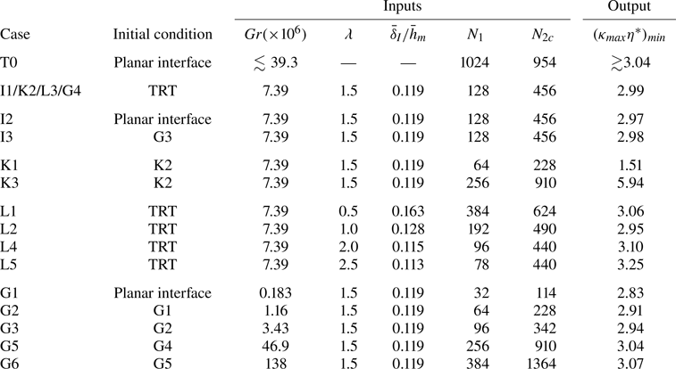
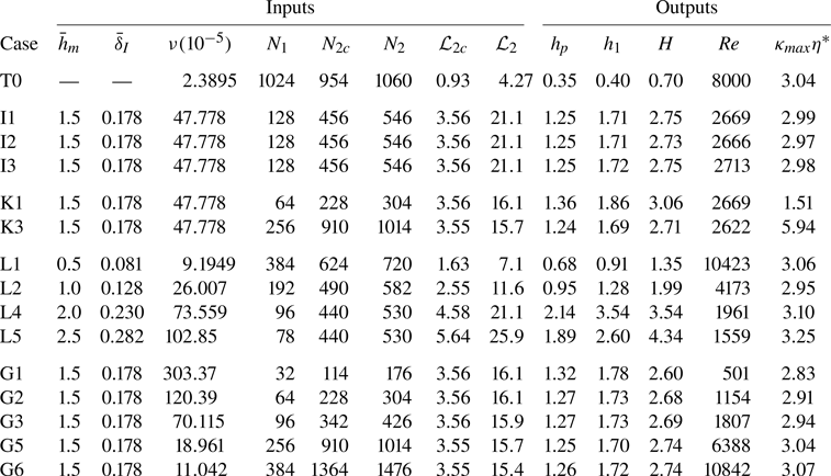
A list of the simulation cases conducted is summarized in table 3 (with more detailed parameters provided in Appendix B). Case T0 simulates the temporal growth of an RT mixing layer using the primitive NSE from an initially perturbed planar interface. Following a similar procedure to Cook et al. (Reference Cook, Cabot and Miller2004), the mass fraction is initialized as
 \begin{equation} Y(\boldsymbol{x}) = \frac{1}{2}\left[ 1 + {\rm erf}\left( \frac{x_2}{\delta_t} + \psi(x_1,x_3) \right)\right], \end{equation}
where the initial thickness of the interface is  $\delta _t = 0.0025{\mathcal {L}}$ and
 $\psi (x_1,x_3)$ is a field of random isotropic perturbations with a Gaussian spectrum centred at
 $\kappa _0=64{\rm \pi} /{\mathcal {L}}$ and standard deviation
 $\sigma _\kappa = \kappa _0/6$. The perturbation field is normalized so that its root-mean-square value is
 $\psi _{rms} = 0.01$. Based on the results from Cabot & Cook (Reference Cabot and Cook2006), both the growth and mixedness parameters seem to settle into their self-similar values by
 $Re = \dot {H}H/\nu \approx 2000$. Separately, the flow may experience lateral confinement effects as the layer height approaches the lateral domain length (Dalziel et al. Reference Dalziel, Patterson, Caulfield and Coomaraswamy2008; Boffetta et al. Reference Boffetta, De Lillo and Musacchio2012a). To minimize these effects, we apply an upper limit of
 $H(t)/{\mathcal {L}} \approx 0.72$, which is deduced from the final simulation time of Cabot & Cook (Reference Cabot and Cook2006) (details are shown in Appendix C). Viscosity and grid parameters are chosen to ensure that a sufficient range of
 $Re(t) \ge 2000$ is well resolved within these
 $H(t)$ limits. Case T0 serves three objectives. First, we validate our numerical framework against other TRT results found in the literature. Second, the self-similar scaling assumption of the SRT equations is verified. Third, T0 is used as a basis for detailed comparisons with subsequent SRT simulations, which differ only in their mathematical framework but maintain consistency in numerical methods, grid resolution, normalizations and flow conditions.
List of simulation cases.

In the remaining cases, the SRT equations are solved. Each of these cases is labelled with a prefix representing the parameter that is varied, i.e. ‘I’ for initial condition, ‘K’ for  $\kappa _{max}\eta ^*$, ‘L’ for aspect ratio
 $\lambda$ and ‘G’ for Grashof number. With the exception of ‘I’ cases, the accompanying number scales with the magnitude of the parameter being studied. Case I1/K2/L3/G4 has multiple labels because it is a part of multiple parametric studies.
The effect of initial conditions on SRT flow is studied using I1–I3. Case I1 is first evolved as a TRT flow from the initial conditions stated in (4.2) with the same perturbation spectrum and initial thickness. Once the target height is reached, the SRT equations are solved. Case I2 is initialized as (4.2) and evolves entirely via the SRT equations. Finally, I3 is initialized by interpolating a fully developed statistically stationary snapshot from G3, an SRT flow of the same height but smaller Grashof number.
Different grid resolutions are considered to examine the effect of numerical errors on the simulation results. Grid resolution is quantified using  $\kappa _{max}\eta ^*$, where
 $\kappa _{max} (\xi _2) = {\rm \pi} /\varDelta _2(\xi _2)$ is the maximum resolved wavenumber, and
 $\eta ^*$ is the Kolmogorov scale, estimated as
 \begin{equation} \eta^*(\xi_2) = \left[\frac{\langle \rho^* \rangle \nu^3}{\langle \rho^* \epsilon^* \rangle}\right]^{1/4}, \quad \langle \rho^*\epsilon^*\rangle = \left\langle \tau^*_{ij}\frac{\partial u^*_i}{\partial \xi_j}\right\rangle. \end{equation}
In SRT flow,  $\kappa _{max} \eta ^*$ varies with
 $\xi _2$, and table 3 provides the minimum values. Grid resolution effects are studied for
 $1.5\lesssim \kappa _{max}\eta ^* \lesssim 6.0$ using K1–K3 and reported in Appendix D. In summary,
 $\kappa _{max} \eta ^*\approx 3$ is deemed sufficient, and is used as a target spatial resolution for all cases. This resolution is also similar to the final time of Cabot & Cook (Reference Cabot and Cook2006).
The final two sets of simulations address the effects of the physical input parameters identified in § 3.2. As discussed,  $A$ and
 $\textit {Sc}$ are not varied. The effect of the mixing layer aspect ratio is studied at constant
 ${\textit {Gr}}$ using simulations L1–L5, corresponding to
 $0.5\le \lambda \le 2.5$. Lastly, the effect of Grashof number is studied at constant
 $\lambda =1.5$ using simulations G1–G6, for Grashof numbers up to
 ${\textit {Gr}} = 1.39\times 10^8$.
5. Results: analysis of SRT framework
In this section, we verify large-scale self-similarity in TRT flow, demonstrate the convergence of SRT flows to stationarity and validate the simplifying assumptions used to derive the SRT equations. The effect of different physical inputs on SRT flow will be studied in § 6. Throughout §§ 5 and 6, comparisons will be made with Cabot & Cook (Reference Cabot and Cook2006) and subsequent analysis of the same dataset (Livescu et al. Reference Livescu, Ristorcelli, Gore, Dean, Cabot and Cook2009; Chung & Pullin Reference Chung and Pullin2010; Zhou & Cabot Reference Zhou and Cabot2019), which may be referred to as the ‘reference’ TRT dataset.
5.1. Temporally growing Rayleigh–Taylor mixing layer
The results from TRT simulation T0 are presented here. In § 5.1.1, different growth regimes of T0 are identified. In § 5.1.2, the data from the self-similar phase are used to validate the scaling assumptions of the SRT equations.
5.1.1. Self-similar growth in TRT
Since TRT flow is non-stationary and homogeneous in the horizontal directions, it is customary to estimate ensemble averages with planar averages, i.e.  $\langle {\cdot } \rangle (t,x_2) = \langle {\cdot } \rangle _{1,3}(t,x_2)$. However, this may result in profiles with significant statistical noise. To mitigate this issue, we leverage self-similar scaling and average results over a small time window,
 $t_1< t< t_2$. Specifically, dimensional data are averaged first in the horizontal directions, then normalized using self-similar scaling, and finally averaged over a small time window. For example, the ensemble-averaged normalized kinetic energy is computed as
 \begin{equation}
\biggl[\frac{\langle \rho u_i^2/2 \rangle}{\rho_0Agh_p}\biggr]_{TRT}\left(t,\frac{x_2-\delta_I}{h_p}\right)
= \left\langle \frac{\langle \rho u_i^2/2 \rangle_{1,3}(t,(x_2-\delta_I)/h_p(t))}{\rho_0Agh_p(t)}
\right\rangle_{t_1\le t\le t_2}.
\end{equation}
The assumed scaling is only valid if the flow is indeed self-similar. In the general case, a small time window is used simply to reduce statistical noise. However, in the self-similar growth regime, larger time windows can be used.
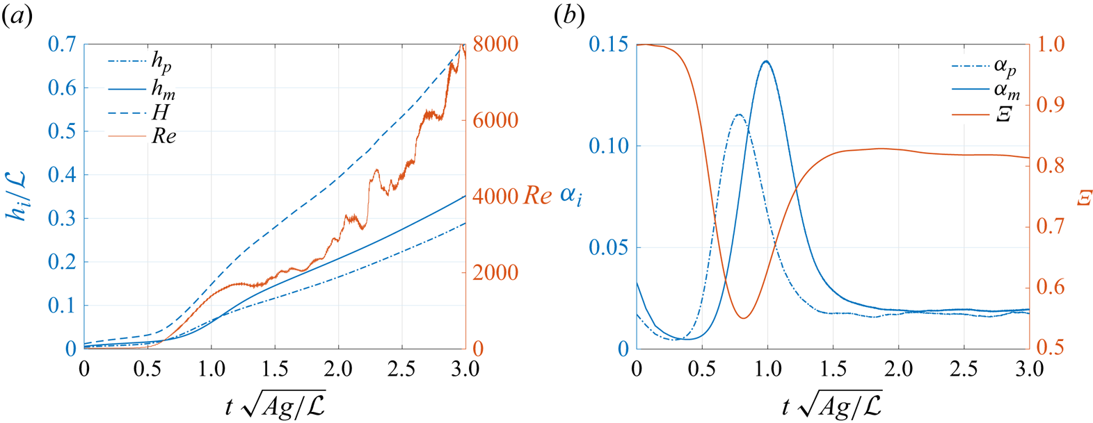
Case T0 is initialized as a perturbed planar interface, and its mathematical description is detailed in § 4.2. Large wavenumber perturbations ( $\ell _I \ll h(t)$) are chosen to encourage late-time self-similar growth that is driven by mode-coupling processes. The time evolution of several quantities derived from the density field is shown in figure 1. Because there is no constant characteristic time scale in TRT, time is non-dimensionalized by
 $({\mathcal {L}}/Ag)^{1/2}$, an arbitrary choice of no physical significance. In figure 1(a), the mixing layer growth is represented by three different height definitions (defined in table 1):
 $h_p$ is the product height that will be used for comparisons with Cabot & Cook (Reference Cabot and Cook2006);
 $h_m$ is the mixing height that will be used as an input parameter to the SRT equations; and
 $H$ is a threshold-based height.
Temporal evolution for TRT-T0: (a) normalized heights and Reynolds number; (b) growth and mixedness parameters. Height definitions are summarized in table 1.

To minimize domain confinement effects, simulations were stopped shortly after  $H(t)/{\mathcal {L}}>0.7$. The height
 $H(t)$ is also used to compute the Reynolds number,
 $Re=H\dot {H}/\nu$. Because
 $H$ is determined from averages over a plane, it is more susceptible to noise than integral height definitions like
 $h_p$ or
 $h_m$. Its time derivative
 $\dot {H}$ is computed using a second-order finite difference in time, which exacerbates statistical noise and contributes to significant fluctuations in
 $Re$. Nonetheless, a growing Reynolds number is clearly observed. The largest
 $Re$ considered in this simulation, attained at
 $t(Ag/{\mathcal {L}})^{1/2} = 3$, is approximately 8000.
The integral heights  $h_p$ and
 $h_m$ from figure 1(a) are normalized using self-similar scaling (1.3) to obtain the growth parameters,
 $\alpha _i = \dot {h}_i^2/(4 A g h_i)$, shown in figure 1(b). The mixedness parameter
 $\varXi$ is defined identically to Cabot & Cook (Reference Cabot and Cook2006) as
 \begin{equation} \varXi =
\frac{1}{h_p}\int^\infty_{-\infty} 2 \langle \min(X,1-X) \rangle \,{\rm d}\kern0.7pt x_2.
\end{equation}
A diffusion-dominated regime is observed for  $t(Ag/{\mathcal {L}})^{1/2} \lesssim 0.2$, where the flow is almost fully mixed at
 $\varXi \approx 1$ and the growth parameter decreases. Subsequently, RT instabilities cause large-amplitude changes in all parameters before the flow transitions to turbulence and reaches quadratic self-similar growth at
 $t(Ag/{\mathcal {L}})^{1/2} \ge 2$. While more sophisticated data analysis techniques can be used to quantify the extent of flow self-similarity (Morgan et al. Reference Morgan, Olson, White and McFarland2017), the self-similar phase in T0 is identified visually by the stationary behaviour of key statistical parameters. This onset of self-similar growth happens at
 $Re \approx 3000$. Although
 $Re \approx 2000$ was identified in § 4.2 as a lower bound for observed self-similarity in Cabot & Cook (Reference Cabot and Cook2006), figure 1(b) shows that this is true for
 $\alpha _p$, but not for
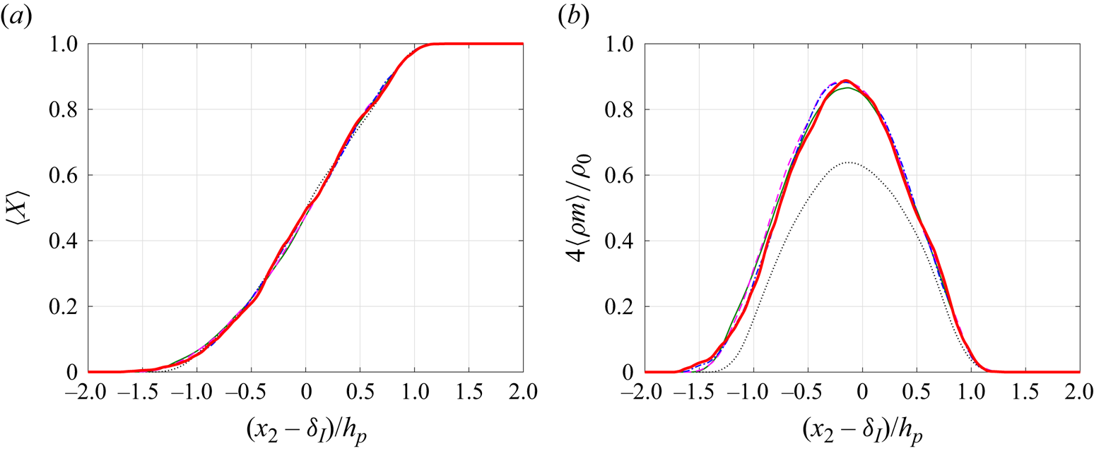
 $\alpha _m$. Indeed, it is well known that not all statistics in TRT flow achieve self-similar behaviour at the same time. Figure 2 shows one-dimensional scalar statistics and further illustrates this: in figure 2(a), the average mole fraction
 $\langle X \rangle$ appears to be converged by
 $t(Ag/{\mathcal {L}})^{1/2} = 1$, while the local mixed mass in figure 2(b) only converges around
 $t(Ag/{\mathcal {L}})^{1/2} = 1.5$.
Temporal evolution for TRT-T0: (a) heavy fluid mole fraction; (b) normalized local mixed mass. Lines represent  $t(Ag/{\mathcal {L}})^{1/2} = 1.0$ (black dotted), 1.5 (green solid), 2.0 (magenta dashed), 2.5 (blue dash-dotted), 3.0 (red thick solid), corresponding to
 $Re \approx 1400$, 1900, 2800, 4400, and 8000, respectively. One-dimensional profiles are first normalized, then averaged over
 $t(Ag/{\mathcal {L}})^{1/2} \pm 0.1$ to reduce statistical variability.

For the purposes of comparison with Cabot & Cook (Reference Cabot and Cook2006) and subsequent SRT results,  $2\le t(Ag/{\mathcal {L}})^{1/2} \le 3$ is taken as the time window where the scalar field exhibits self-similarity. Time averages are calculated over this window to yield
 $\alpha _m = 0.0190$,
 $\alpha _p = 0.0173$ and
 $\varXi = 0.814$. Values of
 $\alpha _p$ and
 $\varXi$ were extracted from figures 4 and 6 of Cabot & Cook (Reference Cabot and Cook2006) and averaged over time for
 $Re>3000$. These values,
 $\alpha _p \approx 0.019$ and
 $\varXi \approx 0.82$, compare well with those obtained from case T0.
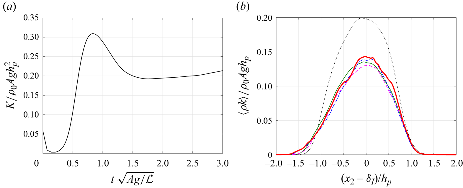
Next, the velocity statistics of T0 are examined. Figure 3(a) shows the time evolution of vertically integrated kinetic energy,  $K = \int ^{+\infty }_{-\infty } \langle \rho k \rangle \,{\rm d}\kern0.7pt x_2$, where
 $k=u_iu_i/2$, while figure 3(b) shows the planar-averaged profiles. Figure 3(a) illustrates that the normalized total kinetic energy has a small positive slope for
 $t(Ag/{\mathcal {L}})^{1/2} \ge 2$, indicating that the velocity statistics of T0 may not be fully self-similar, despite stationarity in
 $\alpha _i$ values. This faster-than-self-similar growth is also observed in the normalized one-dimensional profiles shown in figure 3(b), where the magnitudes continue to increase (albeit slowly) for
 $t(Ag/{\mathcal {L}})^{1/2} \ge 2$.
Temporal evolution of normalized kinetic energy for TRT-T0: (a) vertically integrated; (b) planar averaged. Lines represent  $t(Ag/{\mathcal {L}})^{1/2} =1.0$ (black dotted), 1.5 (green solid), 2.0 (magenta dashed), 2.5 (blue dash-dotted), 3.0 (red thick solid), corresponding to
 $Re \approx 1400$, 1900, 2800, 4400 and 8000, respectively. One-dimensional profiles are first normalized, then averaged over
 $t(Ag/{\mathcal {L}})^{1/2} \pm 0.1$ to reduce statistical variability.

Although T0 does not demonstrate true self-similarity in velocity, the onset of slow growth in normalized kinetic energy aligns with the time window for scalar self-similarity. Hence, the same time window,  $2\le t(Ag/{\mathcal {L}})^{1/2} \le 3$, is used to compute approximately self-similar velocity statistics for subsequent comparisons. Convergence to self-similarity in TRT is a complex issue that depends on the initial conditions and the specific flow statistic considered. It is beyond the scope of this paper to question the existence of true velocity self-similarity in TRT flow. We simply note that T0 exhibits faster-than-self-similar growth in velocity statistics for
 $2\le t(Ag/{\mathcal {L}})^{1/2} \le 3$ and bear this result in mind through subsequent sections.
5.1.2. A priori verification of SRT equations using TRT data
An important objective of the SRT flow configuration is to reproduce TRT flow dynamics. Although the derivation of the SRT equations is informed fundamentally by observations of self-similarity in TRT flow, the statistical equivalence of SRT and TRT flow, stated mathematically as (2.49), has not been demonstrated. Contrary to TRT flow, the time derivative of any ensemble-averaged quantity in a converged SRT flow is zero and is instead replaced by contributions from  $S_\phi$ and
 $T_i$. For (2.49) to hold, the additional SRT terms must, on average, be exactly the negative of the time derivative in TRT flow. We derive the analytical mixed mass and kinetic energy budgets for SRT, assume the validity of (2.49) by evaluating the budget terms from T0 data, and verify that the contributions from
 $S_\phi$ and
 $T_i$ can indeed mimic the time derivative.
In the stationary state, the balance of local mixed mass for SRT can be obtained from (2.46) by setting the time derivative to zero. This is written as
 \begin{equation} 0 ={-} \frac{\partial \langle \rho^* m^*u^*_2\rangle}{\partial \xi_2} + \frac{\partial}{\partial \xi_2}\left\langle \rho^* D \frac{\partial m^*}{\partial \xi_2}\right\rangle + \langle \rho^* \chi^* \rangle + \left(\frac{1}{\tau_0}\xi_2+\delta'_0\right)\frac{\partial \langle \rho^* m^*\rangle}{\partial \xi_2}. \end{equation}
We assume relationship (2.49) and express (5.3) using TRT quantities, leading to
 \begin{equation} 0 = \left[-\frac{\partial \langle \rho mu_2\rangle}{\partial x_2} + \frac{\partial}{\partial x_2}\left\langle \rho D \frac{\partial m}{\partial x_2}\right\rangle + \langle \rho \chi \rangle \right]_{t=t_0} + \left[\frac{1}{\tau_0}(x_2-\delta_I)\frac{\partial \langle \rho m\rangle}{\partial x_2}\right]_{t=t_0}. \end{equation}
The first three terms of (5.4) are precisely the right-hand side of the TRT mixed mass budget shown in (2.17). Their sum is exactly the time derivative of  $\langle \rho m \rangle$. The final term in (5.4) is simplified using relations for
 $\tau _0$ and
 $\delta _0'$ from (2.50) and (2.51). Hence
 \begin{equation} \left[\frac{\partial \langle \rho m\rangle}{\partial t} \right]_{t=t_0} ={-}\left[\frac{\dot{h}_m}{h_m}(x_2-\delta_I)\frac{\partial \langle \rho m\rangle}{\partial x_2}\right]_{t=t_0}. \end{equation}
The SRT term  $S_\phi$ contributes a mixed mass transport term that is exactly the negative of the TRT time derivative at
 $t=t_0$. Both terms of (5.5) are computed from T0 data over the self-similar region, normalized by
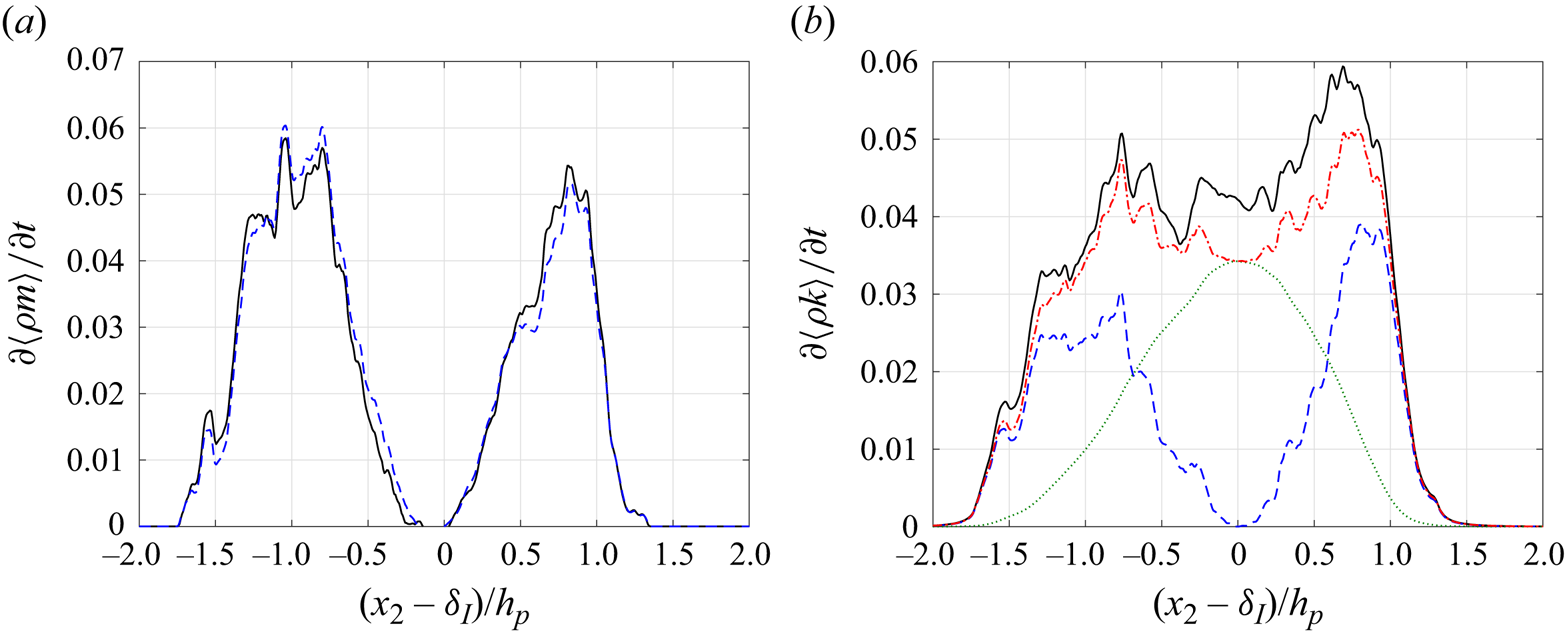
 $\rho _0 (Ag/h_p)^{1/2}$, and shown in figure 4(a). The comparison in figure 4(a) shows that the right-hand side of (5.5) recovers the time derivative of the mixed mass convincingly.
Verification of SRT scaling assumptions using TRT-T0 data, normalized and averaged over  $2.0\le t(Ag/{\mathcal {L}})^{1/2} \le 3.0$. Left-hand side and right-hand side terms from (5.5) and (5.8) are compared. (a) Mixed mass: time derivative (black solid); right-hand side of (5.5) (blue dashed). (b) Kinetic energy: time derivative,
 ${\mathcal {T}}$ (black solid);
 ${\mathcal {T}}_S$ (blue dashed);
 ${\mathcal {T}}_T$ (green dotted);
 ${\mathcal {T}}_S + {\mathcal {T}}_T$ (red dash-dotted).

The same analysis is applied to the kinetic energy budget, which includes contributions from both  $S_\phi$ and
 $T_i$. The TRT kinetic energy budget is derived by multiplying (2.2) by
 $u_i$ and invoking continuity to yield
 \begin{equation} \frac{\partial \langle \rho k \rangle }{\partial t} ={-} \frac{\partial \langle \rho k u_2\rangle }{\partial x_2} - \left \langle u_i \frac{\partial p}{\partial x_i} \right\rangle + \frac{\partial \langle u_i \tau_{i2}\rangle}{\partial x_2} - \left\langle \tau_{ij} \frac{\partial u_i}{\partial x_j}\right\rangle - \langle \rho u_2 \rangle g. \end{equation}
The kinetic energy balance for converged SRT flow can be derived similarly by multiplying (2.34) with  $u^*_i$, and setting the time derivative to zero. This results in
 \begin{align} 0 &={-} \frac{\partial \langle \rho^* k^* u^*_2\rangle }{\partial \xi_2} - \left \langle u_i^*\frac{\partial p^*}{\partial \xi_i} \right\rangle + \frac{\partial \langle u^*_i \tau^*_{i2}\rangle}{\partial \xi_2} - \left\langle \tau^*_{ij} \frac{\partial u^*_i}{\partial \xi_j}\right\rangle- \langle \rho^* {u^*_2} \rangle g \nonumber\\ &\quad + \left(\frac{1}{\tau_0}\xi_2 + \delta'_0\right)\frac{\partial \langle\rho^* k^*\rangle}{\partial \xi_2} - \frac{1}{\tau_0}\langle \rho^* k^*\rangle , \end{align}
where  $k^* = u^*_iu^*_i/2$. After applying assumption (2.49) on (5.7) and substituting (5.6), we get
 \begin{equation} \underbrace{\left[ \frac{\partial \langle \rho k \rangle }{\partial t} \right]_{t=t_0}}_{{\mathcal{T}}(t_0)} = \underbrace{\left[ -\frac{\dot{h}_m}{h_m} (x_2-\delta_I) \frac{\partial \langle\rho k \rangle}{\partial x_2}\right]_{t=t_0}}_{{\mathcal{T}}_S(t_0)} + \underbrace{\left[ \frac{\dot{h}_m}{h_m} \langle\rho k\rangle \right]_{t=t_0}}_{{\mathcal{T}}_T(t_0)}, \end{equation}
where  $\tau _0$ and
 $\delta _0'$ are expressed in terms of
 $h_m$ and
 $\delta _I$ using (2.50) and (2.51). The two terms on the right-hand side of (5.8) represent length and velocity scaling contributions, respectively.
The terms of (5.8) are computed from T0 data, normalized by  $\rho _0(Ag)^{3/2}h_p^{1/2}$, and shown in figure 4(b). Both
 ${\mathcal {T}}_S$ and
 ${\mathcal {T}}_T$ contribute substantially to the estimate of the time derivative, with
 ${\mathcal {T}}_S$ being important near the edges of the mixing layer and
 ${\mathcal {T}}_T$ dominating near the core. The sum of both terms underestimates the time derivative, with a maximum difference of 17 % at
 $x_2\approx \delta _I$. Since the SRT equations are derived on the assumption of self-similarity in velocity, it is not surprising that the SRT terms underestimate the time derivative of T0, a flow that is experiencing faster-than-self-similar velocity growth (see figure 3).
5.2. Stationarity in the SRT configuration
The time evolution of SRT flow is studied using cases I1–I3. These cases have the same  $\lambda =1.5$ and
 ${\textit {Gr}} = 7.4\times 10^6$, but start from different initial conditions, as detailed in § 4.2.
Figure 5(a,b) shows different height definitions that represent the large-scale growth of the mixing layer, while figure 5(c,d) shows the integrated scalar and viscous dissipation, respectively, as representations of the small-scale evolution. In these figures, ensemble averages are estimated with planar averages. After an initial transient, all cases exhibit statistical stationarity in all quantities. Case I1 is initialized with a TRT flow whose mixing height is approximately the input height, hence there are no noticeable changes in any of the quantities computed from I1. Case I2 is initialized as a perturbed flat interface. All quantities in I2 start from small values and grow to their statistically stationary values. Because  $h^*_m$ is actively controlled via the update of
 $\tau _0$ according to closure equation (3.1), it approaches an approximately constant value in a manner consistent with (3.2). In contrast,
 $h^*_p$ responds via the flow dynamics of the SRT equations and oscillates to a greater extent. Case I3 is initialized with an SRT flow of the same height but a smaller
 ${\textit {Gr}}$. The dissipation integrals start from smaller values, but take less than one
 $\tau _0$ to grow to their stationary values. Beyond
 $5\tau _0$, all three signals are indistinguishable. The time-averaged results for
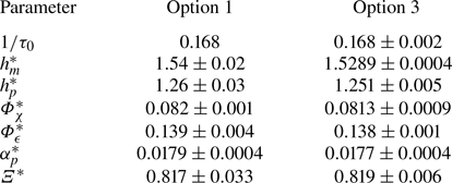
 $s>5\tau _0$ are summarized in table 4, with uncertainties computed using the method presented in Rah & Blanquart (Reference Rah and Blanquart2019). It is clear that the stationary solution does not depend on the initial conditions.
Evolution of normalized (a) mixing height, (b) product height, (c) scalar dissipation integral and (d) viscous dissipation integral for different initial conditions. Insets are zoomed in on early times to highlight differences in the initial transient. The initial conditions used in the SRT cases (I1–I3) correspond respectively to: TRT (red solid); perturbed flat interface (blue dashed); and lower  ${\textit {Gr}}$ SRT (green dash-dotted).

Effect of initial conditions on SRT for  ${\textit {Gr}} = 7.4\times 10^{6}, \lambda = 1.5$.

These results have two practical implications. First, because the initial conditions of an SRT flow do not affect its stationary solution, initializations may be chosen to maximize efficiency without regard for their effect on the final results. Second, leveraging flow stationarity, all ensemble quantities that are extracted from SRT simulations are averaged in both homogeneous directions and time. Each SRT simulation is performed for at least  $50\tau _0$ and statistics are collected after
 $5\tau _0$. Mathematically,
 $\langle {\cdot } \rangle _{SRT} = \langle {\cdot } \rangle _{1,3,s>5\tau _0}$.
5.3. Validity of the SRT equations
Three key assumptions are used in the derivation of the SRT equations. Assumption (III) was verified in § 5.1 through stationarity in  $\alpha (t)$; assumption (II) was verified in § 5.2 through stationarity of all flow quantities in the SRT configuration. In this section, the validity of assumption (I) is assessed. To justify assumption (I), we first propose a candidate for how large this ‘small window of time’ needs to be, then quantify the errors incurred by the SRT simplifications over this time window.
5.3.1. Integral time scale
In § 5.2, it is shown that the flow loses memory of its initial conditions. Stated differently, the flow field loses its time correlation. To quantify how quickly this occurs, temporal autocorrelation functions and integral time scales of several global quantities are computed from I1. These are computed from SRT simulations, as the flow must be statistically stationary and sampled over long times. The temporal autocorrelation function for a general time-varying quantity  $F^*(s)$ is
 \begin{equation} R(\tau) = \frac{\langle {F^*}(s+\tau){F^*}(s)\rangle_s}{\langle {F^*}^2\rangle_s}. \end{equation}
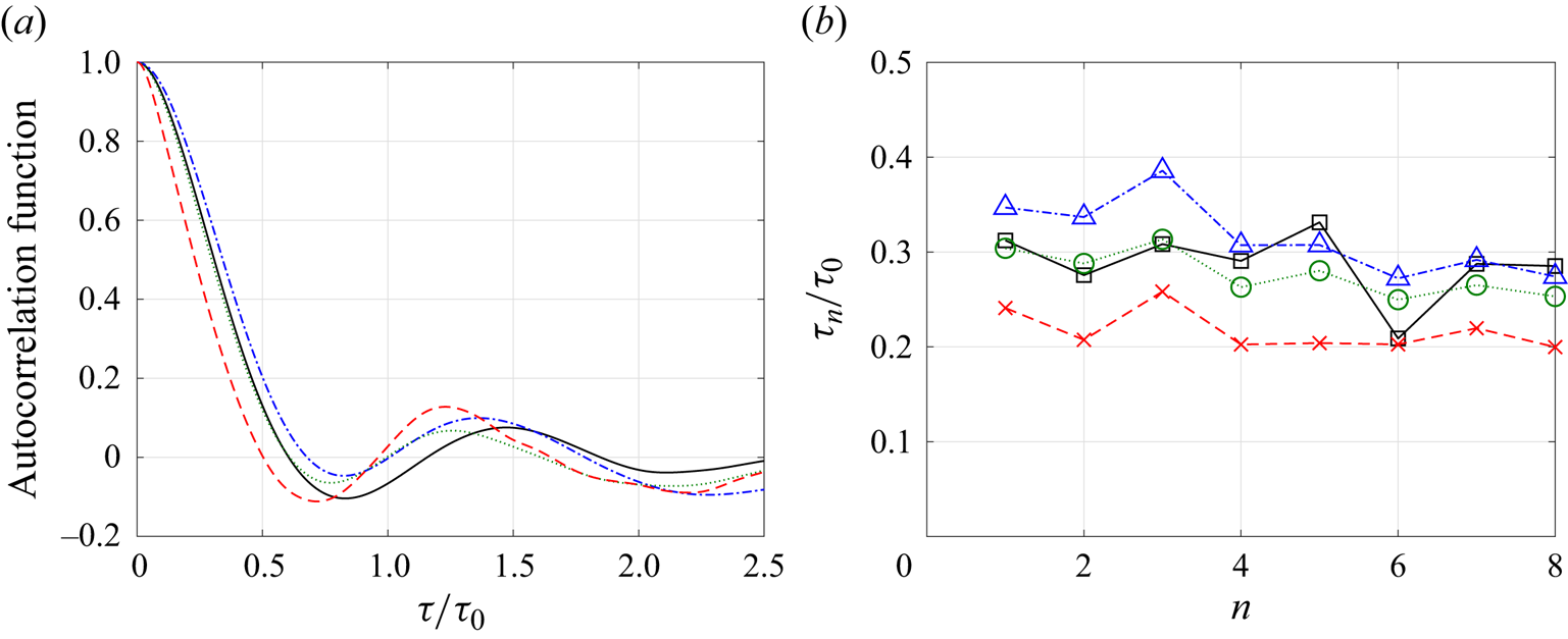
Autocorrelation functions are computed and shown in figure 6(a) for  $F^* = h_p^*,K^*, \varPhi _\epsilon ^*$ and
 $\varPhi _\chi ^*$. All quantities become significantly uncorrelated by
 $\tau \approx \tau _0$. To quantify this more specifically, integral time scales are computed for each of these functions.
(a) Autocorrelation functions from simulation I1 and (b) corresponding integral time scales computed as the integral of  $R(\tau )$ up to the
 $n$th zero crossing. Legend:
 $h_p^*$ (black solid line, squares);
 $K^*$ (blue dash-dotted, triangles);
 $\varPhi _\epsilon ^*$ (green dotted, circles); and
 $\varPhi _\chi ^*$ (red dashed, crosses).

The integral time scale is defined as  $\tau _{int} = \int ^\infty _0 R(\tau ) \,{\rm d}\tau$. Since these time signals (and their autocorrelation functions) have finite lengths,
 $\tau _{int}$ is estimated with an integral up to the
 $n$th zero crossing of the autocorrelation function,
 $\tau _{int}\approx \tau _n$. The integral time scale of each quantity is estimated for varying
 $n$ and shown in figure 6(b). In general,
 $\tau _n$ varies with the choice of quantity and decreases slowly with
 $n$. A conservative upper bound is taken as
 $\tau _{int}\approx 0.4\tau _0$. After
 $\tau _{int}$, flow states become uncorrelated, and a subsequent, independent realization of the flow begins. Hence, the SRT approximations need to be valid for a time window bounded by
 $t_0\pm \tau _{int}/2$.
5.3.2. Error in mixed mass transport and kinetic energy
Recall that the SRT equations are derived from the NSE in § 2.2 through two main steps. The original NSE, (2.1)–(2.3), are first transformed to the rescaled NSE, (2.23)–(2.25), then simplified to the final SRT equations, (2.33)–(2.35), by evaluating them at  $q(t)=q_0$ based on assumption (I). Assessing the validity of assumption (I) is equivalent to quantifying the magnitude of the terms that are neglected even though
 $q\neq q_0$. The SRT errors in mixed mass and kinetic energy transport are estimated by comparing the budget terms evaluated at
 $q(t_0\pm \tau _{int}/2)$ (rescaled TRT) with those at
 $q(t_0)$ (SRT).
First, assumption (III) is used to relate  $q(t_0\pm \tau _{int}/2)/q_0$ to
 $\tau _{int}/\tau _0$. Differentiating (2.32) in time yields
 $q'' = 2\alpha _q A g$, and
 $q^{(n)}=0$ for
 $n>2$. The function
 $q(t)$ can be written as an exact Taylor series, which leads to
 \begin{equation} \frac{q(t_0\pm \tau_{int}/2)}{q_0} = \frac{1}{q_0}\Bigg( q_0 \pm q_0'\frac{\tau_{int}}{2} + q_0''\frac{\tau_{int}^2}{8}\Bigg) = 1 \pm \frac{1}{2}\frac{\tau_{int}}{\tau_0} + \frac{1}{16}\left( \frac{\tau_{int}}{\tau_0}\right)^2. \end{equation}
Substituting  $\tau _{int}/\tau _0 = 0.4$, we obtain
 $0.81\le q/q_0 \le 1.21$.
The SRT errors in mixed mass and kinetic energy budgets are estimated by comparing budgets for the RNSE ( $0.81\le q(t)/q_0 \le 1.21$) and the SRT equations (
 $q=q_0$). The full RNSE budgets and their derivations are found in Appendix E. They are concisely stated as
 \begin{gather} \frac{\partial \langle \rho^* m^* \rangle}{\partial s} ={-} \frac{\partial \langle \rho^* m^*u^*_2\rangle}{\partial \xi_2} + \frac{\partial }{\partial \xi_2}\left\langle \rho^* D \frac{\partial m^*}{\partial \xi_2}\right\rangle + \langle \rho^* \chi^* \rangle + \left(\frac{\xi_2}{\tau_0}+\delta'_0\right)\frac{\partial \langle \rho^* m^*\rangle}{\partial \xi_2} + H_m(t), \end{gather}
 \begin{align}
\frac{\partial \langle\rho^*k^*\rangle}{\partial s} &={-}
\frac{\partial \langle \rho^* k^* u^*_2\rangle }{\partial
\xi_2} - \left \langle u_i^*\frac{\partial {p^*}'}{\partial
\xi_i} \right\rangle + \frac{\partial \langle u^*_i
\tau^*_{i2}\rangle}{\partial \xi_2} - \langle
\rho^*\epsilon^*\rangle - \langle (\rho^*-\langle \rho^*
\rangle) {u^*_2} \rangle g \nonumber\\ &\quad +
\left(\frac{\xi_2}{\tau_0} + \delta'_0\right)\frac{\partial
\langle\rho^* k^*\rangle}{\partial \xi_2} - \frac{\langle
\rho^* k^*\rangle}{\tau_0} + H_k(t).
\end{align}
The first four terms on the right-hand side of (5.11) constitute the full SRT ( $q=q_0$) mixed mass budget. They represent convective transport, diffusive transport, scalar dissipation and the SRT source terms contribution, respectively. The first seven terms on the right-hand side of (5.12) constitute the full SRT kinetic energy budget. They represent convective transport, pressure transport, viscous transport, viscous dissipation, production by buoyancy, and source term contributions from length and velocity scaling, respectively. The final term of each budget equation,
 $H_m$ and
 $H_k$, is the only term that depends on
 $q(t)$, and represents the error of the SRT equations. In figure 7(a,b), these error terms are compared with their corresponding SRT budget terms and shown to be much smaller for both budgets considered. Therefore, they can be neglected without significant impact on the overall flow dynamics.
Comparison of SRT budgets with their  $q(t)$-dependent errors: (a) mixed mass, normalized by
 $\rho _0(Ag/h_p^*)^{1/2}$: convection (red circles); scalar dissipation (green triangles); SRT source term (blue squares); mixed mass diffusion is negligible (not shown). (b) Kinetic energy, normalized by
 $\rho _0(Ag)^{3/2}h_p^{*1/2}$: convection (red circles); viscous dissipation (green triangles); SRT source terms (blue squares); production (orange crosses); pressure transport (magenta solid line, no symbols); viscous transport is negligible (not shown). In both panels, dashed and dotted black lines represent the total error for
 $q/q_0 = 0.81$ and
 $1.21$, respectively.

6. Results: flow physics
Finally, the SRT flow configuration is leveraged to study the effect of various physical inputs. In § 3, four non-dimensional physical inputs were identified. In this section, the Atwood and Schmidt numbers are held constant to facilitate comparisons with Cabot & Cook (Reference Cabot and Cook2006), while the effects of the mixing layer aspect ratio and the Grashof number are presented.
6.1. Effect of mixing layer aspect ratio
The effect of mixing layer aspect ratio,  $\lambda =\bar {h}_m/{\mathcal {L}}$, on SRT is shown qualitatively in figure 8. At all
 $\lambda$ considered, the two reservoirs of pure heavy and light fluid are separated by a highly mixed region that exhibits three-dimensional, random and multiscale features commonly observed in turbulent flows. Consistently, the largest flow structures appear to occupy the entire lateral domain width. For wider (small
 $\lambda$) configurations, sharp interfaces between pockets of heavy and light fluid are evident in many areas, a feature that disappears with enhanced mixing observed in the narrower (large
 $\lambda$) configurations.
Density fields for SRT cases L1–L5 at  ${\textit {Gr}} = 7.4\times 10^{6}$, with increasing mixing layer aspect ratios from left to right:
 $\lambda = 0.5$, 1.0, 1.5, 2.0, 2.5. Images are rescaled to have the same
 $h_m^*$, and non-mixed regions of the flow in the vertical direction are intentionally removed. Blue and red regions correspond to
 $\rho _H$ and
 $\rho _L$, respectively.

The role of the lateral domain size  ${\mathcal {L}}$ is different in TRT and SRT flows. In self-similar TRT flow, Zhou & Cabot (Reference Zhou and Cabot2019) showed that both vertical and horizontal length scales of the flow grow at approximately fixed ratios to the mixing layer height. The TRT flow configuration is solved over a finite time, and domains can be chosen to be sufficiently large (relative to the finite time window) so that they do not affect the flow. Unlike TRT, SRT flow is designed to be simulated over infinitely long times. Vertical growth is restricted by
 $\bar {h}_m$ but lateral growth is not; horizontal length scales can grow continuously until they are constrained by the lateral domain width if there are no other fluid dynamical constraining mechanisms. As lateral length scales approach the size of the domain, the flow physics is affected by the periodic lateral boundaries. In other stationary configurations of both isotropic (Rosales & Meneveau Reference Rosales and Meneveau2005; Dhandapani & Blanquart Reference Dhandapani and Blanquart2020) and buoyant (Chung & Pullin Reference Chung and Pullin2010; Carroll & Blanquart Reference Carroll and Blanquart2015) turbulent flows, integral turbulence length scales have similarly been shown to depend on the domain dimensions.
To quantify this behaviour, additional flow length scales, similar to Zhou & Cabot (Reference Zhou and Cabot2019), are computed. The correlation length  $\varLambda ^*_i$ is defined as the integral of the longitudinal autocorrelation function, i.e.
 \begin{equation} \varLambda^*_i = \int^\infty_0 C_i(r) \,{\rm d}r, \quad C_i(r) = \frac{\langle {u^*_i}' (s,\boldsymbol{\xi} + \boldsymbol{e}_i r) {u^*_i}'(s,\boldsymbol{\xi})\rangle}{\langle {u^*_i}'^2 \rangle}, \end{equation}
with no sum over index  $i$ (where
 $i=1, 2$ or 3), and
 ${u_i^*}' = u_i^* - \langle u_i^*\rangle$. Since the flow is periodic in
 $\xi _1$ and
 $\xi _3$, the horizontal correlation lengths can be defined in terms of their energy spectra as
 \begin{equation}
L^*_i = \left.{\displaystyle\int^\infty_0 \kappa^{{-}1}
E^*_i(\kappa) \,{\rm d}\kappa}\right/{\displaystyle\int^\infty_0
E^*_i(\kappa)\,{\rm d}\kappa},
\end{equation}
where  $E^*_i(\kappa )$ is the two-dimensional spectral energy density of
 $u^*_i$, and
 $\kappa$ is the two-dimensional wavenumber in the horizontal plane. To characterize the layer core,
 $L_1^*$ and
 $L_3^*$ are computed on the
 $\xi _2$-plane closest to
 $\delta ^*_I$. Zhou & Cabot (Reference Zhou and Cabot2019) verified that definitions (6.1) and (6.2) are approximately equivalent, hence,
 $\varLambda ^*_i$ and
 $L^*_i$ can be treated interchangeably in the horizontal directions.
The correlation lengths are shown in figure 9(a,b) as a function of  $\lambda$. The normalized correlation lengths in both the vertical and horizontal directions decrease as the mixing layer aspect ratio is increased. Consistent with visual observations in figure 8, the lateral domain size physically restricts the growth of horizontal length scales in the SRT configuration. A less obvious consequence is that the vertical correlation length also decreases in a similar fashion, despite being normalized by the mixing layer height. Unlike TRT, SRT flow is affected independently by a second large length scale,
 ${\mathcal {L}}$. Hence, a mapping of SRT domain length scales to observed flow length scales is necessary for comparison with TRT.
Effect of mixing layer aspect ratio on normalized (a) vertical and (b) horizontal correlation lengths, (c) growth and (d) mixedness parameters. Red markers represent SRT values at  ${\textit {Gr}}=7.4\times 10^6$; the maximum and minimum values from TRT simulations (
 $Re>3000$) are shown as: T0 (black dashed); reference dataset (Cabot & Cook Reference Cabot and Cook2006; Zhou & Cabot Reference Zhou and Cabot2019) (blue dotted).

Time-averaged TRT values (corresponding to  $Re>3000$) for
 $\varLambda _2$ and
 $L_{1,3}$ are extracted from figure 13 of Zhou & Cabot (Reference Zhou and Cabot2019) and T0. Due to significant statistical variation, these are shown as maximum and minimum values in figure 9. Figure 9(a) shows that
 $\varLambda _2/h_p$ from both TRT sources are well matched by SRT at
 $\lambda =1.5$. Figure 9(b) shows a much larger spread of
 $L_{1,3}/h_p$ values from the TRT data. Arguably, all
 $L^*_{1,3}/h^*_p$ values from the SRT simulations of
 $0.5 \le \lambda \le 2.0$ are within the statistical variation of the two TRT simulations. There are two reasons for this larger statistical variation. First,
 $L_{1,3}$ is computed from spectra on a single plane, it is expected to be less converged than
 $\varLambda _2$, which is computed from an integral over the full domain. Second, in both Zhou & Cabot (Reference Zhou and Cabot2019) and T0, it is observed that
 $L_{1,3}/h_p$ continues to decrease slowly with time. Because the matching of
 $L_{1,3}/h_p$ values is inconclusive, the excellent agreement in
 $\varLambda _2/h_p$ is the main criterion for selecting
 $\lambda =1.5$ as the SRT configuration that corresponds best with TRT growth.
Additionally, supporting evidence of the  $\lambda =1.5$ SRT configuration being an equivalent flow unit to self-similar TRT can be found in the spectra of Cabot & Cook (Reference Cabot and Cook2006). A wavenumber corresponding to the peaks of the vertical velocity and density spectra,
 $k_{peak}$, is extracted from figure 2 of Cabot & Cook (Reference Cabot and Cook2006) and used to estimate an aspect ratio,
 $h_p k_{peak}/2{\rm \pi} \approx 1.2$. This compares well with the value of
 $h_p^*/{\mathcal {L}}\approx 1.25$ for SRT at
 $\lambda = 1.5$. Hence, it appears that the lateral domain width of the SRT configuration may be dynamically equivalent to the most energetic lateral wavelength in TRT flow.
Finally, the effect of the mixing layer aspect ratio is examined in terms of the growth parameter  $\alpha ^*_p$ and mixedness
 $\varXi ^*$. Although SRT is statistically stationary, a growth parameter,
 $\alpha _m^*= \alpha _m (t_0)$, corresponding to a TRT mixing layer at
 $h_m(t_0)$ can be computed using the SRT parameter
 $\tau _0$. Evaluating the definition of
 $\alpha _m$ at
 $t=t_0$, and using (2.50), we can relate the TRT growth parameter to SRT flow quantities with
 \begin{equation} \alpha^*_m = \alpha_m(t_0) = \left. \frac{1}{4Ag} \frac{\dot{h}_m^2}{h_m} \right|_{t=t_0} = \frac{h_m^*}{4Ag} \left( \frac{1}{\tau_0} \right)^2. \end{equation}
It is then corrected for different height definitions using
 \begin{equation} \alpha^*_i = \alpha^*_m \frac{h^*_i}{h^*_m} = \frac{h_i^*}{4Ag} \left( \frac{1}{\tau_0} \right)^2. \end{equation}
The mixedness parameter for TRT is defined in (5.2) and  $\varXi ^*$ has an identical definition, differing only in the coordinate system used. Figure 9(c,d) shows that the SRT values at
 $\lambda =1.5$ match self-similar TRT values from Cabot & Cook (Reference Cabot and Cook2006) and T0 well, verifying that SRT can reproduce TRT flow statistics as long as the correlation lengths are matched.
By matching the statistical flow length scales between SRT and TRT, we identify the SRT configuration with  $\lambda =1.5$ as being representative of self-similar TRT flow (for
 $A=0.5$ and
 $\textit {Sc}=1$). This is verified by good agreement in
 $\alpha _p$ and
 $\varXi$ values. This configuration will be referred to as SRT-1.5 in the subsequent sections.
6.2. Effect of Grashof/Reynolds number
The effect of Grashof number on SRT-1.5 is studied. As discussed in § 3.2,  ${\textit {Gr}}\propto Re^2$ for a self-similar flow, and either quantity can be used to characterize turbulence intensity. Since
 $Re$ is more commonly used in TRT studies, all results are presented in terms of
 $Re$ (defined in (1.4) and (3.7)) for ease of comparison. The * superscript may be omitted when comparing SRT and TRT quantities, as the specific definition should be clear from the context.
The effect of  $Re$ (or
 ${\textit {Gr}}$) on SRT flow is shown qualitatively in figure 10. All cases have the same
 $\bar {h}_m$ and
 ${\mathcal {L}}$. Visually, the largest length scales observed are similar across all Reynolds numbers. Expectedly, the largest vertical scale is constrained by
 $\bar {h}_m$ and the largest horizontal scale is constrained by
 ${\mathcal {L}}$. In contrast, the smallest length scales in the flow decrease noticeably with Reynolds number. Additionally, three-dimensional mixing is observed across all
 $Re$. For small
 $Re$, this mixing primarily manifests through a smearing of the large-scale interfaces via laminar diffusion. For large
 $Re$, this mixing process is driven by the generation of small-scale turbulent structures.
Density fields for SRT cases G1–G6 at  $\lambda = 1.5$ and increasing Reynolds (or Grashof) number from left to right:
 $Re \approx 500$, 1200, 1800, 2700, 6400 and 10 800. Non-mixed regions of the flow in the vertical direction are intentionally removed. Blue and red regions correspond to
 $\rho _H$ and
 $\rho _L$, respectively.

Figure 11 shows the variation of several key parameters with  $Re$ for both SRT and TRT flow. Besides
 $\alpha _p$ and
 $\varXi$, we examine two other parameters,
 $K/\delta P$ and
 $\eta$. The ratio of kinetic-to-potential energy is defined using the vertically integrated kinetic energy
 $K(t)$ and the loss of potential energy relative to the initial state:
 \begin{align} \delta P(t) & = \int^{\infty}_{-\infty} \langle \rho(\boldsymbol{x}, t=0) - \rho(\boldsymbol{x}, t)\rangle g x_2\, {\rm d}\kern0.7pt x_2 \end{align}
 \begin{align} & \approx g\Bigg[\int^{\infty}_0 \langle \rho_H-\rho \rangle x_2 \,{\rm d}\kern0.7pt x_2 + \int^0_{-\infty} \langle \rho_L-\rho \rangle x_2 \,{\rm d}\kern0.7pt x_2 - \frac{\rho_H-\rho_L}{2} \delta^2_I\Bigg]. \end{align}
We compute  $\delta P$ using (6.6), which is exactly equal to (6.5) if the initial interface is assumed to be infinitely thin. The corresponding definitions of
 $K^*$ and
 $\delta P^*$ for SRT are similar, with the appropriate variable substitution. The Kolmogorov length scale
 $\eta$ presented in figure 11(d) is the minimum value of
 $\eta$ found in the mixing layer. It is normalized by the mixing layer height and compared against the expected Kolmogorov scaling.
Comparison of SRT-1.5 with two different sources of TRT as a function of Reynolds number: SRT-1.5 (red squares); TRT-T0 (black points); data extracted from Cabot & Cook (Reference Cabot and Cook2006) (blue solid line). (a) Growth parameter; (b) mixedness; (c) ratio of kinetic to potential energy; (d) normalized Kolmogorov length scale ( $Re^{-3/4}$ line represents Kolmogorov scaling).

Both SRT and TRT approach similar behaviour at high Reynolds numbers. The parameters  $\alpha _p$ and
 $\varXi$ approach statistically stationary values,
 $K/\delta P$ exhibits a slow growth and
 $\eta$ scales in accordance with Kolmogorov scaling. We note that both sets of TRT data predict a lower
 $K/\delta P$ than SRT-1.5 and exhibit slightly faster growth than SRT-1.5 for
 $Re>2000$; it is likely that both TRT simulations have not achieved self-similarity in velocity. This will be addressed in greater detail in § 6.3. While the general high
 $Re$ behaviour between SRT and TRT flow is similar, the manner in which this self-similar state is approached is drastically different. A distinct change in flow regime is observed at
 $Re \approx 2000$ for TRT, corresponding to the onset of self-similar growth discussed in § 5.1.1. In contrast, the values in SRT approach high
 $Re$ behaviour smoothly. Because SRT is independent of initial conditions and enforces self-similar behaviour through timewise recycling, SRT flow decouples memory effects from
 $Re$ effects, leading to the possibility of low Reynolds number self-similar RT mixing.
6.3. Detailed comparisons between SRT and TRT turbulence
In this section, a more detailed comparison of SRT-1.5 and TRT is performed. We first present planar-averaged statistics for G1–G6 to examine  $Re$ effects, then proceed to compare self-similar results from G5, T0 and the Cabot & Cook (Reference Cabot and Cook2006) dataset where available.
It was shown in § 6.2 that the global quantities of both TRT and SRT-1.5 show minimal Reynolds number sensitivity for  $Re \gtrsim 3000$. We compare G5 (
 $Re^*\approx 6400$) and the self-similar region of T0 (
 $3000 \lesssim Re \lesssim 8000$). Statistics from T0 are first normalized, then averaged over this time window. Although the reference dataset has a much larger
 $Re$ range that reaches up to 32 000, we expect the results between all three simulations to compare relatively well after quantities are suitably normalized. One-dimensional profiles are extracted from Livescu et al. (Reference Livescu, Ristorcelli, Gore, Dean, Cabot and Cook2009) when available. Due to the limited number of snapshots presented, an approximate spread corresponding to all data in the range
 $Re>3000$ is shown. This spread represents the maximum and minimum values of the normalized profiles observed at each
 $x_2$ location.
A qualitative comparison of SRT-1.5 and TRT-T0 density fields at  $Re \approx 6400$ is shown in figure 12. Both flow fields look similar, revealing a similar range of length scales and flow features. Movie 1 shows the time evolution for case G5. After the flow evolves from its lower
 ${\textit {Gr}}$ initial state to higher
 ${\textit {Gr}}$ behaviour by
 $s\approx \tau _0$, the flow appears stationary, ergodic and similar to TRT flow. Additionally, we note that the mixing layer aspect ratio for SRT-1.5 is approximately 4 times that of the TRT configuration. For the same
 $Re$, each in-plane direction for SRT flow is 4 times smaller, resulting in a sixteenfold reduction in the total number of grid points. This has obvious computational benefits that will be further discussed in § 7.2.
Comparison of TRT-T0 and SRT-1.5 (G5) density fields for  $Re\approx 6400$. Images are rescaled to have the same
 $h_m$, and non-mixed regions of the flow in the vertical direction are intentionally removed.

The average heavy fluid mole fraction profiles are compared between SRT-1.5 and TRT. Figure 13(a) shows the variation of  $\langle X \rangle$ with Reynolds number for SRT-1.5. These profiles show almost no sensitivity to
 $Re$, even at very low Reynolds numbers. Case G5 is compared with TRT results in figure 13(b). There are minor differences in the shape of these profiles, with both sources of TRT data having slightly extended tails towards the outer edges of the mixing layer. Next, the average local mixed mass is considered. The variation of mixed mass with Reynolds number for SRT-1.5 is shown in figure 14(a). Profile shapes are similar across different
 $Re$. Magnitudes are within 5 % across the entire range and converge smoothly towards high
 $Re$. Figure 14(b) shows that the average local mixed mass of TRT-T0 compares well with SRT-1.5, but with minor deviations at the tails similar to figure 13(b).
Heavy fluid mole fraction. (a) Reynolds number effects on SRT-1.5 at  $Re^* \approx 500$ (red dotted), 1200 (blue dash-dotted), 1800 (magenta solid), 2700 (green dashed), 6400 (thick red solid) and 10 800 (thick black dashed). (b) Comparison of SRT-G5 (red), TRT-T0 (black dashed) and approximate spread from Livescu et al. (Reference Livescu, Ristorcelli, Gore, Dean, Cabot and Cook2009) (blue shaded).

Normalized mixed mass. (a) Reynolds number effects on SRT-1.5 at  $Re^* \approx 500$ (red dotted), 1200 (blue dash-dotted), 1800 (magenta solid), 2700 (green dashed), 6400 (thick red solid) and 10 800 (thick black dashed). (b) Comparison of SRT-1.5 G5 (red) and TRT-T0 (black dashed).

The differences at the outer edges of the mixing layer may be attributed to a deviation from self-similarity in TRT flow. In TRT flow, the outer edges of the mixing layer are characterized by a small number of isolated mushroom-shaped structures with laminar fronts that extend primarily in a single direction (bubbles move up; spikes move down). Examples of these isolated structures are noticeable in the TRT snapshot towards the bottom of figure 12. These structures are most likely to retain some properties of the initial conditions. In contrast, SRT flow retains no memory of the initial perturbations and self-similar mixing is experienced throughout the entire domain.
Next, the normalized planar-averaged kinetic energy is considered. Figure 15(a,b) shows the  $Re$ dependence of SRT-1.5 and a comparison with TRT, respectively. Shapes of kinetic energy profiles are largely similar across
 $Re$ but there appears to be a weak
 $Re$ dependence in the peak magnitudes. In figure 15(b), SRT-1.5 is compared with T0 at a similar Reynolds number. Similar to trends observed in the scalar statistics, SRT-1.5 has shorter tails than T0. Additionally, the peak magnitude is 14 % larger than the corresponding value from T0. Although figure 15(b) compares only G5 with T0, it can be easily compared with figure 15(a) to show that T0 has a lower peak than SRT-1.5 for the entire range of
 $Re$. This is consistent with the smaller values of
 $K/\delta P$ for TRT across all
 $Re >2000$ in figure 11(c). This discrepancy might be attributed to the fact that the SRT equations are designed to enforce velocity self-similarity, but T0 has not in fact reached a state of velocity self-similarity. It was shown in § 5.1 that normalized velocity statistics continue to grow for T0. It is likely that the SRT-1.5 kinetic energy profiles represent an upper limit for TRT and the profiles for TRT may eventually converge to this limit if T0 is simulated for a longer time window.
Normalized kinetic energy. (a) Reynolds number effects on SRT-1.5 at  $Re^* \approx 500$ (red dotted), 1200 (blue dash-dotted), 1800 (magenta solid), 2700 (green dashed), 6400 (thick red solid) and 10 800 (thick black dashed). (b) Comparison of SRT-G5 (red) and TRT-T0 (black dashed).

Finally, we consider the anisotropy of the velocity field using the anisotropy tensor
 \begin{equation} {\mathsf{b}}_{ij} = \frac{\langle \rho u_i u_j \rangle}{\langle \rho u_k u_k \rangle} - \frac{1}{3}\delta_{ij}, \end{equation}
of which, the  ${\mathsf{b}}_{22}$ component is shown in figure 16(a,b). A value of 0 describes isotropic behaviour and a value of 2/3 represents pure one-dimensional vertical flow. Equation (6.7) involves a ratio of velocities, and these approach zero in the reservoirs. Hence, values of
 ${\mathsf{b}}_{22}$ near and beyond the edges of the mixing layer should not be overly scrutinized. Figure 16(a) shows that anisotropy increases toward the outer edges of the mixing layer and decreases with
 $Re$. In the layer core,
 ${\mathsf{b}}_{22}$ converges to approximately 0.27 at high Reynolds number. Although magnitudes differ, profile shapes are similar even at low
 $Re$ and converge smoothly toward high
 $Re$. In figure 16(b), the anisotropy of SRT-1.5 is compared with TRT. Both sources of TRT data have slightly larger values of
 ${\mathsf{b}}_{22}$ compared with SRT-1.5. However, trends are similar and magnitudes are not significantly different. In addition, because the velocity statistics of the TRT simulations may not yet be fully self-similar, it is possible that the anisotropy of the TRT cases could converge to SRT-1.5 values with longer simulation times.
Anisotropy. (a) Reynolds number effects on SRT-1.5 at  $Re^* \approx 500$ (red dotted), 1200 (blue dash-dotted), 1800 (magenta solid), 2700 (green dashed), 6400 (thick red solid) and 10 800 (thick black dashed). (b) Comparison of SRT-G5 (red), TRT-T0 (black dashed) and approximate spread from Livescu et al. (Reference Livescu, Ristorcelli, Gore, Dean, Cabot and Cook2009) (blue shaded).

6.4. Higher-order statistics
To verify that the SRT framework preserves the spatial structure of RT turbulence, two-point statistics are considered. Two-dimensional spectra  $E_i(\kappa )$ are computed using SRT-G5 data at
 $x_2 = \delta _I$ (or
 $\xi _2 = \delta ^*_I$), where
 $E_i(\kappa )$ is the two-dimensional spectral energy density of
 $u_i$, and
 $\kappa$ is the two-dimensional wavenumber in the horizontal plane. The spectrum for vertical velocity is
 $E_2$, and the spectrum for horizontal velocity is computed as
 $(E_1+E_3)/2$. Equivalent spectra are computed from TRT-T0 for a similar
 $Re\approx 6400$ and both sets of data are compared in figure 17(a). The SRT and TRT spectra show good agreement throughout the entire range of scales. Consistent with Cabot & Cook (Reference Cabot and Cook2006), an inertial range resembling Kolmogorov
 $\kappa ^{-5/3}$ scaling is observed in the
 $E_2$ spectrum, but not in the horizontal directions. The smallest wavenumber in the SRT spectra is approximately four times as large as that of TRT, due to the difference in domain sizes. The smallest wavenumber in SRT flow corresponds exactly to the most energetic wavenumber of TRT flow. This observation is not a coincidence; the SRT configuration acts as a minimum flow unit for RT turbulence, and this will be discussed in § 7.1.
Spectra comparison between TRT-T0 and SRT-G5 at  $Re\approx 6400$ on horizontal plane
 $x_2\approx \delta _I$. (a) Two-dimensional spectra for vertical and horizontal velocities: TRT
 $E_2$(black solid); TRT
 $(E_1+E_3)/2$ (black dashed); SRT
 $E^*_2$ (blue circles); SRT
 $(E^*_1+E^*_3)/2$ (red squares). (b) Anisotropy spectra: TRT (black dashed); SRT (red solid); and approximate spread from Chung & Pullin (Reference Chung and Pullin2010) at
 $Re \approx 32\,000$ (blue shaded).

The structure of the small scales is further examined using the anisotropy spectrum
 \begin{equation} B_i(\kappa) = \frac{E_i}{E_1+E_2+E_3}-\frac{1}{3}, \end{equation}
and computed from SRT-G5 and TRT-T0 data. The two spectra are shown in figure 17(b), alongside an approximate spread of the equivalent spectrum for the Cabot & Cook (Reference Cabot and Cook2006) dataset that is found in figure 13 of Chung & Pullin (Reference Chung and Pullin2010). All three sets of data seem to suggest an increase in anisotropy in the dissipation range towards the smaller scales, albeit with some differences in magnitudes. The values from SRT-G5 are bounded by those of TRT-T0 and the reference data, verifying that SRT flow reproduces similar spectra to TRT flow. Differences in the two sets of TRT results may be related to initial conditions and/or Reynolds number, but it is difficult to conclude without further study.
Finally, we verify that SRT flow can also capture localized, irregular behaviour by comparing its intermittency characteristics with TRT flow. A procedure similar to Boffetta et al. (Reference Boffetta, Mazzino, Musacchio and Vozella2009) is used. In one dimension, the  $p$th-order longitudinal velocity structure function is
 \begin{equation} S_p(r) = \langle (u_i(x_i+r) - u_i(x_i))^p \rangle. \end{equation}
These are computed at  $x_2\approx \delta _I$ using
 $u_1(x_1)$ and
 $u_3(x_3)$, and averaged over the plane in both horizontal directions. The structure functions for
 $p=$ 2, 4 and 8 are shown in figure 18(a).
(a) Longitudinal velocity structure functions for  $p=$ 2 (circles), 4 (triangles) and 8 (plus signs) for SRT-G5 at
 $\xi _2=\delta ^*_I$. Symbols represent SRT data and dashed lines correspond to the scaling exponents
 $3\zeta _p/p = 1.0$, 0.97 and 0.84, respectively. (b) Relative scaling exponents computed using the ESS method based on their deviation from
 $S_3(r)$: SRT-G5 (red squares); TRT-T0 (black circles); data from Boffetta et al. (Reference Boffetta, Mazzino, Musacchio and Vozella2009) (blue crosses); Kolmogorov's four-fifth law (dashed green line); assumed
 $\zeta _3=1$ (filled symbol).

Turbulence intermittency can be quantified by computing the scaling exponents,  $S_p(r)\propto r^{\zeta _p}$, from the data. A deviation of
 $\zeta _p$ from
 $p/3$ is commonly considered evidence of turbulence intermittency (Anselmet et al. Reference Anselmet, Gagne, Hopfinger and Antonia1984; Meneveau & Sreenivasan Reference Meneveau and Sreenivasan1987). However, obtaining these scaling exponents requires power-law fitting over the limited inertial ranges that are found in the current simulations. The extended self-similarity (ESS) procedure from Benzi et al. (Reference Benzi, Ciliberto, Tripiccione, Baudet, Massaioli and Succi1993) is used to overcome this issue. The premise of this procedure is that the dissipation range can also be used in the power-law fitting after it is normalized by the third-order structure function. In doing so,
 $\zeta _3=1$ is assumed.
The computed relative scaling exponents are shown in figure 18(b) for both SRT-G5 and TRT-T0, and the respective fits are reflected in figure 18(a) for comparison with the original SRT structure functions. The scaling exponents from SRT-G5 and TRT-T0 show good agreement, suggesting that SRT flow is able to capture a similar level of intermittency that is present in TRT flow. Although Boffetta et al. (Reference Boffetta, Mazzino, Musacchio and Vozella2009) studied the RT configuration at a much lower Atwood number (in the Boussinesq approximation), the scaling exponents are extracted from figure 4 of their study and shown in figure 18(b) for comparison purposes. There is little difference between all the results compared, suggesting that Atwood number may not affect the scaling exponents of the structure functions significantly.
7. Discussion
In § 7, a comparison of the TRT and SRT frameworks is considered from two broad perspectives. First, the physical relationship between SRT and TRT flows is explored in § 7.1. Then, the computational benefits of the SRT configuration are discussed in § 7.2.
7.1. Minimal flow unit for self-similar RT turbulence
The results reviewed in § 6 suggest that the SRT configuration with  $\lambda =1.5$ represents a minimal flow unit for self-similar TRT turbulence in the mode-coupling limit. The idea of a ‘minimal flow unit’ has mostly been used in the context of wall-bounded turbulence (Jiménez & Moin Reference Jiménez and Moin1991; Hamilton, Kim & Waleffe Reference Hamilton, Kim and Waleffe1995; Hsieh & Biringen Reference Hsieh and Biringen2016), and is extended analogously to the RT configuration here. This flow unit is considered ‘minimal’ because the
 $\lambda =1.5$ domain isolates a single unit of the largest energetic structures present in self-similar RT turbulence, as illustrated by the spectra in figure 17(a).
The relatively high aspect ratio SRT minimal flow unit proposed here is not a contradiction to existing findings regarding the effect of lateral confinement on TRT flow (Dalziel et al. Reference Dalziel, Patterson, Caulfield and Coomaraswamy2008; Boffetta et al. Reference Boffetta, De Lillo and Musacchio2012a). In TRT flow,  ${\mathcal {L}}_{TRT}$ is a fixed physical domain. In contrast,
 ${\mathcal {L}}_{SRT}$ is a simulation domain that is always scaled by the height of the mixing layer, and unrelated to any physical domain in the TRT sense. As
 $s\rightarrow \infty$, flow structures in the SRT configuration have a tendency to fill out the lateral domain while maintaining a statistically stationary height. Flow stationarity is expected only after the onset of lateral confinement effects. The SRT minimal flow unit leverages the expected lateral confinement effects to select the aspect ratios of RT flow structures and ‘recycles’ them at a constant aspect ratio. In the context of a self-similar TRT flow, many statistically equivalent realizations of
 $\lambda =1.5$ units are tiled horizontally (figure 19). Each of them can be imagined to be expanding at constant aspect ratio, interacting and merging with other neighbouring units to form larger
 $\lambda =1.5$ units. In a finite-domain TRT set-up, these units grow in size and eventually experience confinement effects as
 $h_m(t) \sim {\mathcal {L}}_{TRT}$. Because
 ${\mathcal {L}}_{SRT}$ scales with
 $h_m$, the SRT configuration preserves the aspect ratio of these flow units and shields them from any such physical confinement effects, effectively simulating RT turbulence in an infinitely large physical domain.
Illustration of the relationship between SRT-1.5 and a finite-domain TRT flow: at an earlier time,  $t_1$, TRT can be represented as a large number of small SRT units of
 $\lambda =1.5, {\textit {Gr}} ={\textit {Gr}}_1$. There is sufficient scale separation (
 ${\mathcal {L}}_{TRT} \gg {\mathcal {L}}_{SRT}$) to allow for constant aspect ratio growth; at late times, fewer and larger SRT units of
 ${\textit {Gr}}_2>{\textit {Gr}}_1$ fit within the finite TRT domain. As
 ${\mathcal {L}}_{SRT}$ approaches
 ${\mathcal {L}}_{TRT}$, lateral confinement effects begin to modify the nature of RT turbulence.

The SRT-1.5 flow unit represents a theoretical limit at which all memory of initial conditions has been lost, and the physical domain is infinite. Any TRT simulation has to be done on a finite domain over finite time, and it remains questionable if any existing TRT simulation in the literature (as large as they already are) has achieved ‘true’ mode-coupling self-similarity, particularly in velocity statistics. The SRT-1.5 configuration is not a substitute for TRT simulations in all scenarios, especially when the initial conditions or finite-domain effects are of specific interest. It is a configuration for studying late-time self-similar TRT behaviour, and does so using the smallest possible domain.
7.2. Computational benefits
Lastly, we address the computational benefits that are associated with the SRT configuration.
At a given Reynolds number, the computational cost for one timestep at one grid point is marginally higher in the SRT flow configuration. The evaluation of  $\tau _0(s)$,
 $\delta _0'(s)$ and the associated source terms increases the computational time by <1 %. The temporal resolution requirements for both the TRT and SRT configurations are similar. By computing
 $S_\phi$ using (4.1), all additional terms are either evaluated semi-implicitly or are stabilizing at large time scales. Time resolution is determined by the convective CFL condition, which is comparable between SRT and TRT, given the similarity in velocity statistics. The small penalty associated with the computation of the additional SRT terms is far outweighed by the benefits listed below:
(i) Reduced domain size: for the same layer height, the SRT minimal flow unit identified in § 6.1 requires a lateral domain width that is approximately one-fourth that of the TRT simulation reported in Cabot & Cook (Reference Cabot and Cook2006), which translates to a sixteenfold reduction in the total number of grid points for an equivalent flow condition. Granted, due to the smaller number of grid points in each snapshot, multiple snapshots will be required to reach a similar level of statistical convergence. However, memory requirements are significantly reduced and there is greater flexibility in storage and analysis of the data.
(ii) Independence of initial conditions: each TRT simulation has to be initialized from a perturbed flat interface and evolved over its full time history. Unlike TRT flow, SRT flow has been shown in § 5.2 to be insensitive to initial conditions. Hence, thoughtful flow initialization strategies, such as using an existing turbulent simulation of a different
$Re$ as an initial condition, can speed up convergence to the target flow state.(iii) Convergence of ensemble statistics: when simulating TRT flow on a finite domain, self-similarity only develops after an initial transient, and the flow eventually experiences lateral confinement effects. There is a limited time window (if any) for the collection of self-similar TRT statistics. The number of statistical samples can only be increased by using a larger domain or by performing multiple realizations of the same simulation. In contrast, SRT flow is stationary and ergodic. A single flow configuration can theoretically be simulated over infinite time on the same grid to generate an infinite number of realizations, guaranteeing converged estimates of ensemble statistics.
(iv) Reduced
$Re$ requirements for self-similar RT turbulence: finally, self-similar turbulence can be observed robustly at a much lower Reynolds number in SRT flows than in TRT flows. The effects of initial conditions and Reynolds number are intrinsically linked in TRT flow. In contrast, the SRT configuration encourages self-similar behaviour and decouples the two effects, yielding unique statistically stationary solutions defined entirely by $A$, $\textit {Sc}$, ${\textit {Gr}}$ and $\lambda$. This is true even at low $Re$ (or ${\textit {Gr}}$). Additionally, the results in § 6 show that low $Re$ SRT turbulence is qualitatively similar to high $Re$ cases and approaches the high $Re$ limit in a smooth, monotonic fashion. This property makes the SRT configuration a highly scalable test bed for the development of turbulence models for buoyancy-driven flows.


8. Conclusion
Inspired by the observed self-similar behaviour of RT mixing layers, a coordinate transformation was applied to the low-Mach-number NSE to obtain a new set of equations in the rescaled coordinate system. The rescaled governing equations, referred to as the SRT equations, are valid in the vicinity of a fixed time. These equations resemble the original NSE but contain two sets of additional terms; one arises from rescaling of the vertical coordinate and takes a similar form in the continuity, momentum and scalar equations; the second arises from rescaling of velocities and only appears in the momentum equation.
Using the SRT equations, we demonstrated that self-similar TRT turbulence in the mode-coupling limit can be simulated in a statistically stationary manner, circumventing many of the computational challenges typically associated with temporally growing simulations. A minimum flow unit for self-similar RT turbulence (SRT-1.5) was identified, which reveals the underlying structure of such flows. The results from SRT-1.5 match well with TRT simulations, and differences can likely be attributed to the non-self-similar nature of the TRT simulations considered. We propose that SRT-1.5 generates RT turbulence at a theoretical limit corresponding to complete flow self-similarity. This may otherwise only be achieved through TRT simulations with longer times and larger grids than any existing simulation.
Supplementary movie
Supplementary movie is available at https://doi.org/10.1017/jfm.2024.1104.
Acknowledgements
The authors acknowledge the Texas Advanced Computing Center (TACC) at The University of Texas at Austin for providing computational resources that have contributed to the research results reported within this paper. URL: http://www.tacc.utexas.edu.
Funding
This material is based upon work supported by the National Science Foundation under Grant No. 2422513.
Declaration of interests
The authors report no conflict of interest.
Appendix A. Implementation of SRT inputs
The complete SRT equations are defined by (2.33)–(2.35) and require the specification of two parameters  $\tau _0$ and
 $\delta _0'$. After a statistically stationary state is reached, we expect (2.44) and (2.48) to be satisfied. In this section, we outline several options for how this stationary state can be reached through different ways of implementing
 $\tau _0$ and
 $\delta _0'$.
A.1. Choice of $\tau _0$: stability of $h_m^*$


The options for implementing  $\tau _0$ are summarized in figure 20. Option 1t uses a prescribed constant
 $\bar {\tau }_0$ as input to the SRT equations. Both options 2t and 3t use (2.48), with option 2t enforcing instantaneous stationarity, and option 3t driving the flow toward a stationary state at a particular mixing height. We examine the stability of the stationary solution using the
 $h_m^*$ time-evolution equation.
(i) Constant
$\tau _0$ as direct input (option 1t): when a constant value, $\bar {\tau }_0 >0$, is used directly as an input to (2.33)–(2.35), the time evolution of $h_m^*$ can be derived by substituting $\tau _0 = \bar {\tau }_0$ into (2.47) to yield
(A1)Because\begin{equation} \frac{{\rm d}h_m^*}{{\rm d}s} = \frac{4}{\rho_0} \varPhi_\chi^* - \frac{1}{\bar{\tau}_0} h_m^*. \end{equation}$\bar {\tau }_0$ and $h_m^*$ are both positive by definition, the last term on the right-hand side of (A1) is a relaxation term that stabilizes $h_m^*$. $\varPhi _\chi ^*$ is positive by definition, hence the first term is destabilizing. The overall stability of $h_m^*$ depends on the relative scaling of both terms on the right-hand side. In general, this is dependent on the flow physics.(ii) Enforcing instantaneous stationarity (option 2t): the second option uses the stationarity relation derived in § 2.3 to enforce
${\rm d}h_m^*/{\rm d}s = 0$ at all times. This is achieved by updating $\tau _0(s)$ continuously based on (2.48) as
(A2)Because stationarity is satisfied at all times,\begin{equation} \frac{1}{\tau_0(s)} = \frac{4\varPhi_\chi^*(s)}{\rho_0 h_m^*(s)}. \end{equation}$h_m^*$ is completely determined, at least analytically, by its initial state and can only be changed by re-initializing the flow. Moreover, while stationarity is satisfied analytically, it may not be satisfied numerically. Errors may accumulate and $h_m^*$ may drift from its initial value.(iii) Constant mixing height as input (option 3t): finally, option 3t uses a constant mixing width,
$\bar {h}_m>0$, as input to the stationarity relation such that $\tau _0(s)$ is continuously updated as
(A3)Substituting (A3) into (2.47) gives\begin{equation} \frac{1}{\tau_0(s)} = \frac{4 \varPhi_\chi^*(s)}{\rho_0 \bar{h}_m}. \end{equation}(A4)Both\begin{equation} \frac{{\rm d}h_m^*}{{\rm d}s} = \frac{4\varPhi_\chi^*}{\rho_0} \left( 1- \frac{h_m^*}{\bar{h}_m} \right). \end{equation}$\varPhi _\chi ^*$ and $h_m^*$ are positive by definition. This guarantees the relaxation of the instantaneous layer width to the prescribed target value, $h_m^*(s) \to \bar {h}_m$, regardless of its initial state.


Options for implementing  $\tau _0$. Quantities with an overbar (circled) are prescribed constant inputs.

Option 3t is chosen as the input method because it guarantees stability and affords the user flexibility to prescribe a target mixing height that is independent of initial conditions. Practically, an input length scale  $\bar {h}_m$ is also preferred to an input time scale
 $\bar {\tau }_0$ because
 $\bar {h}_m$ can be easily compared with computational (e.g. grid, domain size) and physical length scales (e.g. Kolmogorov scale, other height definitions) when setting up the simulation.
A.2. Choice of $\delta '_0$: stability of $\delta _I^*$


The options for implementing  $\delta _0'$, illustrated in figure 21, are analogous to the ones for
 $\tau _0$. We examine the stability of the stationary solution using the
 $\delta _I^*$ time evolution equation.
(i) Constant
$\delta '_0$ as direct input (option 1d): one way to implement $\delta _0'$ is to use a constant input $\bar {\delta }_0'$ directly with the SRT equations. Equation (2.43) becomes
(A5)Because\begin{equation} \frac{{\rm d}\delta_I^*}{{\rm d}s} ={-}\frac{1}{\tau_0} \delta_I^* - \bar{\delta}_0'. \end{equation}$1/\tau _0 >0$, this is a stable equation and
(A6)The parameter\begin{equation} \delta_I^*(s) \rightarrow - \bar{\delta}_0'\tau_0(s). \end{equation}$\tau _0(s)$ is, in general, a time-varying quantity. Hence, $\delta _I^*(s)$ converges to a time-varying quantity in the statistically stationary state.(ii) Enforcing instantaneous stationarity (option 2d): a second option is to enforce stationarity in
$\delta _I^*$ instantaneously using (2.44) such that ${\rm d}\delta _I^*/{\rm d}s = 0$ for all time, i.e.
(A7)The considerations against option 2d are the same as those for option 2t.\begin{equation} \delta'_0 (s) ={-}\frac{1}{\tau_0}{\delta_I^*(s)}. \end{equation}(iii) Constant displacement length as input (option 3d): as a third option, we use a constant value for the displacement length,
$\bar {\delta }_I$, as input to (2.44), i.e.
(A8)Equation (2.43) becomes\begin{equation} \delta'_0 ={-}\frac{1}{\tau_0}{\bar{\delta}_I}. \end{equation}(A9)\begin{equation} \frac{{\rm d}\delta_I^*}{{\rm d}s} = \frac{1}{\tau_0} (\bar{\delta}_I - \delta_I^*), \end{equation}


which is a stable equation that guarantees  $\delta _I^*(s) \rightarrow \bar {\delta }_I$.
Options for implementing  $\delta '_0$. Quantities with an overbar (circled) are prescribed constant inputs.

Both options 1d and 3d are analytically stable, and enable the mixing layer to be shifted without re-initialization. With option 1d,  $\delta _I^*(s)$ (and hence the total mass) fluctuates in the stationary state. Hence, option 3d is preferred because
 $\delta _I^*(s)$ relaxes to a constant target value that serves as a known reference location for all times.
A.3. Equivalence of implementation options
The choice of implementation does not affect the final result. To demonstrate this, two simulations are compared. Case I1O3 (also I1/K2/L3/G4) is performed using option 3, and a second simulation I1O1 is performed using option 1. Case I1O3 takes  $(\bar {h}_m,\bar {\delta }_I,)$ as inputs and computes
 $(\tau _0(s),\delta _0'(s))$ as outputs, while case I1O1 takes
 $(\tau _0,\delta _0')$ as inputs, and computes
 $(h_m^*(s),\delta _I^*(s))$ as outputs. To verify their equivalence, the time-averaged values of
 $\tau _0(s)$ and
 $\delta _0'(s)$ from I1O3 are used as inputs to I1O1. The time evolution of each of these four quantities is shown in figure 22. For option 3,
 $(h_m^*(s),\delta _I^*(s))$ approach near-constant values consistent with (A4) and (A9), while
 $(\tau _0(s),\delta _0'(s))$ oscillate. For option 1,
 $(\tau _0,\delta _0')$ are constants (as prescribed), and
 $(h_m^*(s),\delta _I^*(s))$ oscillate. These observations are consistent with the time-evolution equations presented in §§ A.1 and A.2.
Comparison of option 1 (blue dashed) and option 3 (red solid). (a) Mixing layer height; (b) SRT time scale parameter; (c) displacement length; (d) SRT translation velocity parameter.

Despite differences in the timewise behaviour of these particular quantities, the ensemble-averaged results from options 1 and 3 are identical to each other, within statistical uncertainty. These are summarized in table 5. There is a unique solution for ensemble-averaged SRT flow, that is controlled by two additional parameters. These can be height  $h^*_m$ and position
 $\delta _I^*$, or time scale
 $\tau _0$ and drift
 $\delta _0'$. Prescribing either set of inputs maps the other to this unique state, resulting in equivalent flows that are independent of how the simulation is implemented.
Comparison of ensemble-averaged results between options 1 and 3.

Appendix B. Detailed simulation parameters
In § 3.2, seven physical inputs ( $g, \rho _H, \rho _L, \nu, D, \bar {h}_m, {\mathcal {L}}$) and four independent dimensionless groups (
 $A, \textit {Sc}, {\textit {Gr}}, \lambda$) were identified. Hence, three of the seven input parameters can be arbitrarily chosen. In our simulations, these are
 $g = \rho _H = {\mathcal {L}}=1$. The remaining four inputs are determined from the choice of
 $A=0.5$,
 $\textit {Sc}=1$,
 ${\textit {Gr}}$ (varied) and
 $\lambda$ (varied). Specific input values and some intermediate outputs are presented in table 6, which serves as an extension to table 3.
Detailed simulation parameters. The T0 outputs are approximate values at the end of the simulation.

Appendix C. Determination of aspect ratio limit for TRT simulation
In TRT simulation T0, the mixing layer aspect ratio (in terms of  $H/{\mathcal {L}}$) is compared with a threshold value to limit lateral confinement effects. This threshold value is deduced from the final simulation time of Cabot & Cook (Reference Cabot and Cook2006). However,
 $H/{\mathcal {L}}$ was not directly reported and had to be derived from other reported parameters. The ratio
 $H/{\mathcal {L}}$ can be expanded as
 \begin{equation} \left(\frac{H}{{\mathcal{L}}}\right)^3 = \frac{1}{2} \left(\frac{H}{h_p}\right) \left(\frac{H\dot{H}}{\nu} \right)^2 \Bigg(\frac{\dot{h}_p}{\dot{H}}\Bigg)^2 \Bigg(\frac{4Agh_p}{\dot{h}_p^2} \Bigg) \Bigg(\frac{\nu^2}{2Ag\varDelta_1^3} \Bigg) \left(\frac{\varDelta_1}{{\mathcal{L}}}\right)^3. \end{equation}
The input computational parameters are quoted explicitly as  ${\textit {Gr}}_\varDelta = (2Ag\varDelta _1^3)/\nu ^2 = 1$, and
 $N = {\mathcal {L}}/\varDelta _1 = 3072$. For a self-similar flow, we assume
 $\dot {H}/\dot {h}_p \approx H/h_p$. The self-similar parameters are
 $\alpha _p = \dot {h}_p^2/(4Agh_p)\approx 0.02$ (extracted from their figure 4) and
 $H/h_p\approx 2.4$ (reported). At the end of the simulation,
 $Re = H\dot {H}/\nu \approx 32 000$. Substituting these values into (C1), we find
 $H/{\mathcal {L}}\approx 0.72$ at the end of the simulation.
Appendix D. Effect of grid resolution on SRT flow
To assess the effects of grid resolution, a parametric sweep of  $\kappa _{max}\eta ^* \approx 1.5, 3, 6$ was conducted for constant
 ${\textit {Gr}}$ and
 $\lambda$ using K1–K3. Table 7 summarizes the results, and shows that grid resolution has an impact on the output values that exceeds the statistical uncertainty.
Effect of grid resolution on SRT for  ${\textit {Gr}} = 7.4\times 10^{6}, \lambda = 1.5$.

Specific attention is placed on  $h^*_m$ because it has a known analytical solution. While (3.2) implies that
 $h^*_m = \bar {h}_m$ in the stationary state, this is not satisfied numerically. The relative deviation of
 $h^*_m$ from its input value is presented in figure 23. Here,
 $h^*_m$ is consistently larger than
 $\bar {h}_m$ and converges towards
 $\bar {h}_m$ with increased resolution. This error can be attributed to numerical diffusion, which exists in any bounded scalar transport scheme. One may mimic the impact of the numerical diffusion
 $D_{num}$ by multiplying the molecular diffusion
 $D$ by a factor
 $(1+D_{num}/D)$. Specifically, (2.47) becomes
 \begin{equation} \frac{{\rm d}h_m^*}{{\rm d}s} \approx \frac{4}{\rho_0} \left(1 + \frac{D_{num}}{D}\right)\varPhi_\chi^* - \frac{1}{\tau_0}h_m^*. \end{equation}
Because  $1/\tau _0$ is updated via (3.1), (D1) becomes
 \begin{equation} \frac{{\rm d}h_m^*}{{\rm d}s} \approx \frac{4\varPhi_\chi^*}{\rho_0} \left(1 + \frac{D_{num}}{D} - \frac{h_m^*}{\bar{h}_m} \right), \end{equation}
and the stationary solution can be written as
 \begin{equation} \frac{D_{num}}{D} \approx \frac{h_m^*-\bar{h}_m}{\bar{h}_m}. \end{equation}
Effect of grid resolution on the deviation of  $h^*_m$ from prescribed input,
 $\bar {h}_m$. For reference, dashed lines have slopes corresponding to second-order (green) and third-order (orange) accuracy.

Hence, the relative error in  $h^*_m$ can provide an estimate for the numerical scalar diffusion present in the flow. Comparing the errors with the reference slopes in figure 23, the error in
 $h_m^*$ exhibits second-order convergence. This is consistent with the order of accuracy of the BCH scheme (Verma et al. Reference Verma, Xuan and Blanquart2014). The BCH scheme was chosen for scalar transport precisely for its reduced numerical diffusion, yet, the numerical diffusivity observed at conventional DNS resolution is significant. Specifically, at
 $\kappa _{max}\eta ^* = 1.5$, numerical diffusion is estimated to be 14 % of physical diffusion. This is expected to be worse with other bounded scalar transport schemes that have larger numerical diffusion. As the grid resolution is increased to
 $\kappa _{max}\eta ^* = 3$, this value is reduced to smaller than 2 %. Taking into account both results from table 7 and figure 23,
 $\kappa _{max}\eta ^* = 3$ is assessed to be sufficient for this study.
Appendix E. Mixed mass and kinetic energy budgets for rescaled TRT flow
E.1. Mixed mass transport in rescaled TRT flow
The ensemble-averaged mixed mass transport equation for rescaled TRT flow (as opposed to SRT flow) is derived in the same way as (2.46), but starting with the full rescaled scalar equation (2.25), instead of the SRT equation (2.35). All ratios involving  $q$,
 $q'$ and
 $q''$ can be written in terms of
 $q/q_0$ using assumption (III), such as
 \begin{align} \frac{q'}{q'_0} = \left(\frac{q}{q_0} \right)^{1/2}, \quad \frac{q'}{q} = \frac{q'}{q'_0}\frac{q'_0}{q_0}\frac{q_0}{q} = \frac{1}{\tau_0}\left(\frac{q_0}{q}\right)^{1/2}, \quad \frac{q''}{q'} = \frac{1}{2}\frac{q'}{q} = \frac{1}{2\tau_0}\left(\frac{q_0}{q}\right)^{1/2}. \end{align}
The mixed mass transport equation derived from the RNSE is
 \begin{align} \frac{\partial \langle \rho^* m^* \rangle}{\partial s} &={-} \frac{\partial \langle \rho^* m^*u^*_2\rangle}{\partial \xi_2} + \frac{\partial }{\partial \xi_2}\left\langle \rho^* D \frac{\partial m^*}{\partial \xi_2}\right\rangle + \langle \rho^* \chi^* \rangle + \left(\frac{\xi_2}{\tau_0}+\delta'_0\right)\frac{\partial \langle \rho^* m^*\rangle}{\partial \xi_2}\nonumber\\ &\quad + H_{c,m} + H_{D,m}+H_\chi+H_{S,m} , \end{align}
where the first four terms on the right-hand side represent convective transport, diffusive transport, scalar dissipation and the SRT source terms contribution, respectively. These four terms constitute the full SRT ( $q=q_0$) mixed mass budget. The additional
 $q(t)$-dependent error terms associated with each of these terms are
 $$\begin{gather} H_{c,m} ={-}\Bigg[\Bigg(\frac{q_0}{q}\Bigg)^{1/2}-1\Bigg] \frac{\partial \langle\rho^* m^*u^*_2\rangle}{\partial \xi_2}, \end{gather}$$
 $$\begin{gather}H_{D,m} = \Bigg[\Bigg(\frac{q_0}{q}\Bigg)^2-1\Bigg] \frac{\partial}{\partial \xi_2}\left\langle \rho^* D \frac{\partial m^*}{\partial \xi_2}\right\rangle, \end{gather}$$
 $$\begin{gather}H_{\chi} = \Bigg[\Bigg(\frac{q_0}{q}\Bigg)^2-1\Bigg] \langle \rho^*\chi^{e*}\rangle, \quad \chi^{e*} = 2D\left(\frac{\partial Y^*}{\partial \xi_2} \right)^2, \end{gather}$$
 $$\begin{gather}H_{S,m} = \Bigg[\Bigg(\frac{q_0}{q}\Bigg)^{1/2}-1\Bigg] \left(\frac{\xi_2}{\tau_0} +\delta_0'\right)\frac{\partial \langle\rho^* m^*\rangle}{\partial \xi_2}. \end{gather}$$
The sum of these error terms is written as  $H_m$ in § 5.3.2. Each term is estimated by assuming that the ensemble averages of the rescaled quantities are constant in time and approximated by SRT flow, i.e. the dominant source of error in time originates from the variation of
 $q(t)/q_0$.
E.2. Kinetic energy transport in rescaled TRT flow
A similar procedure is used to derive the kinetic energy transport equation for the full RNSE. To isolate dynamical pressure effects from the hydrostatic head, pressure is decomposed into a hydrostatic component and a fluctuating component  ${p^*}'$ such that
 $\partial p^*/ \partial \xi _i =\partial {p^*}'/\partial \xi _i - \langle \rho ^*\rangle g \delta _{2i}$. The RNSE kinetic energy budget is
 \begin{align} \frac{\partial
\langle\rho^*k^*\rangle}{\partial s} &={-} \frac{\partial
\langle \rho^* k^* u^*_2\rangle }{\partial \xi_2} - \left
\langle u_i^*\frac{\partial {p^*}'}{\partial \xi_i}
\right\rangle + \frac{\partial \langle u^*_i
\tau^*_{i2}\rangle}{\partial \xi_2} - \langle
\rho^*\epsilon^*\rangle - \langle (\rho^*-\langle \rho^*
\rangle) {u^*_2} \rangle g\nonumber\\ &\quad +
\left(\frac{\xi_2}{\tau_0} + \delta'_0\right)\frac{\partial
\langle\rho^* k^*\rangle}{\partial \xi_2} - \frac{\langle
\rho^* k^*\rangle}{\tau_0}\nonumber\\ &\quad + H_{C,k} + H_{p,k} + H_{\nu,k}
+ H_\epsilon +H_{\mathcal{P}} + H_{S,k} +
H_{T,k}, \end{align}
where the first seven terms on the right-hand side represent convective transport, pressure transport, viscous transport, viscous dissipation, production by buoyancy and source term contributions from length and velocity scaling, respectively. The remaining  $q(t)$-dependent error terms are
 $$\begin{gather} H_{c,k} ={-}\Bigg[\Bigg(\frac{q_0}{q}\Bigg)^{1/2}-1\Bigg] \frac{\partial \langle\rho^* k^*u_2^*\rangle}{\partial \xi_2}, \quad H_{p,k} ={-}\Bigg[\Bigg(\frac{q_0}{q}\Bigg)^{1/2}-1 \Bigg] \left \langle u_i^*\frac{\partial p^*}{\partial \xi_i} \right\rangle, \end{gather}$$
 $$\begin{gather}H_{\nu,k} = \left[\frac{q_0}{q}-1 \right] \left[\frac{\partial \langle u^*_i(\tau_{i2}^*+\tau_{i2}^{e*})\rangle}{\partial \xi_2} + \left(\frac{q_0}{q}-1\right)\frac{\partial \langle u^*_i\tau_{i2}^{e*}\rangle}{\partial \xi_2} \right], \end{gather}$$
 $$\begin{gather}H_{\epsilon} ={-}\left[\frac{q_0}{q}-1 \right] \left[\left\langle \tau_{i2}^* \frac{\partial u_i^*}{\partial \xi_2} + \tau_{ij}^{e*}\frac{\partial u_i^*}{\partial \xi_j}\right\rangle + \left(\frac{q_0}{q}-1\right)\left\langle \tau_{i2}^{e*} \frac{\partial u_i^*}{\partial \xi_2} \right\rangle \right], \end{gather}$$
 $$\begin{gather}H_{\mathcal{P}} ={-}\Bigg[\Bigg(\frac{q_0}{q}\Bigg)^{1/2}-1\Bigg] \langle(\rho^*-\langle \rho^* \rangle)u_2^*g\rangle, \end{gather}$$
 $$\begin{gather}H_{S,k} = \Bigg[\Bigg(\frac{q_0}{q}\Bigg)^{1/2}-1\Bigg] \left(\frac{1}{\tau_0}\xi_2 +\delta_0'\right)\frac{\partial \langle\rho^* k^*\rangle}{\partial \xi_2}, \quad H_{T,k} ={-}\Bigg[\Bigg(\frac{q_0}{q}\Bigg)^{1/2}-1\Bigg] \frac{\langle\rho^* k^*\rangle}{\tau_0}. \end{gather}$$
The sum of these error terms is written as  $H_k$ in § 5.3.2. Similar to the mixed mass budget, we approximate that all
 $t$-dependent errors are dominated by
 $q(t)/q_0$.