From a business cycle perspective, numerous researchers have investigated drivers of the Great Depression, but we are far from agreement and do not have an answer even to a simple question: Was the Great Depression driven by technology shocks or non-technology shocks? Proponents of real-business-cycle (RBC) models, Harold Cole and Lee Ohanian (Reference Cole and Ohanian1999) and Timothy Kehoe and Edward Prescott (Reference Kehoe and Prescott2008), find that, from 1929 to 1933, technology regress measured by standard total factor productivity (TFP) series explains much of observed falls in output in their models. This finding seems surprising, given that many other economists assert the driving role of non-technology shocks: financial system collapse (Bernanke Reference Bernanke1983), higher uncertainty (Romer Reference Romer1990), and tight monetary policy (Bordo, Erceg, and Evans Reference Bordo, Erceg and Evans2000). In contrast, many researchers regard technology improvements as a driver of the recovery. The RBC models of Cole and Ohanian (Reference Cole and Ohanian1999) and Kehoe and Prescott (Reference Kehoe and Prescott2008) predict that technology improvements over the recovery phase cause large increases in employment that return output rapidly to trend. Stephen Cecchetti and Georgios Karras (1994) and Michelle Alexopoulos and Jon Cohen (Reference Alexopoulos and Cohen2009), who use vector autoregression (VAR) models, also find that technology or supply shocks played an important role in the recovery. At the same time, some emphasize the important role of monetary or inflation-expectation channel (Temin and Wigmore Reference Temin and Wigmore1990; Romer Reference Romer1992; Eggertsson Reference Eggertsson2008, Reference Eggertsson2012).
Interest in technology shocks during the Great Depression is not limited to the business cycle literature. From a historical perspective, technology growth in the whole Great Depression period is given prominence by Alexander Field (Reference Field2003, Reference Field2006) who argues that technology improvements over the period 1929–1941 were fastest in the U.S. history. This is especially startling in light of a more than 20-percent fall in gross domestic product from 1929 to 1933. This claim is based on his study of John Kendrick's (Reference Kendrick1961) TFP series and a variety of microeconomic case studies and his results are comprehensively documented in his book (Field, Reference Field2012).
A difficulty in assessing existing studies on pre-WWII technology change is the lack of a reliable measure of historical technology change.Footnote 1 Cole and Ohanian (Reference Cole and Ohanian1999) and Field (Reference Field2003, Reference Field2006, Reference Field2012) use Kendrick's (Reference Kendrick1961) TFP series, which is adjusted partially for reallocation effects arising from input movements across industries, but not for varying input utilization, increasing returns to scale, and imperfect competition. Kehoe and Prescott's (Reference Kehoe and Prescott2008) TFP series is adjusted for none of these factors. While there exists a TFP measure “purified” by Susanto Basu, John Fernald, and Miles Kimball (2006) for the post-WWII period, no such TFP measure exists for the pre-WWII period. The purpose of this article is to construct a new historical measure of technology change and use the new measure to reassess the role of technology change over the Great Depression.
I propose a modified version of Basu, Fernald, and Kimball's (Reference Basu, Clarida, Frankel, Giavazzi and West2006) approach. Using instruments such as monetary and oil shocks, Basu, Fernald, and Kimball (Reference Basu, Clarida, Frankel, Giavazzi and West2006) estimate industry-level production functions, where explanatory variables consist of hours worked per employee as a proxy for unobserved input utilization, in addition to total hours worked, capital stock, and intermediate inputs. They estimate industry technology changes as residuals and aggregate those by industry shares in total value added to measure technology changes in the whole economy. Their approach cannot be directly applied to pre-WWII data, where there are neither industry-level, long-run, annual data for output or inputs, nor aggregate time-series data for intermediate inputs. I also argue that Basu, Fernald, and Kimball's (Reference Basu, Clarida, Frankel, Giavazzi and West2006) instruments appear to work only in post-WWII data. To address these data issues, I use Kendrick's (Reference Kendrick1961, Reference Kendrick1973) data for output and inputs aggregated by industry shares in total value added, follow Basu's (Reference Basu1996) strategy and assume Leontief technology between valued added and intermediate inputs, and suggest new instruments that effectively work in pre-WWII data. The spirit is similar to the work of Robert Inklaar, Herman de Jong, and Reitze Gouma (Reference Inklaar, de Jong and Gouma2011), who propose their own adjustments, though I critically examine their adjustments in this article.
My purified TFP series that covers the period 1892–1966 indicates that, on average, technology improvements continued during the downturn. The large TFP declines found by Cole and Ohanian (Reference Cole and Ohanian1999) and Kehoe and Prescott (Reference Kehoe and Prescott2008) are fully explained by declines in input utilization. Hence, their finding for the driving role of technology regress in the downturn appears to be the result of mismeasurement. The pace of technology improvements from 1934 to 1941 was rapid at 3.4 percent per year on average and more than double of the pre-WWII average of 1.6 percent. Over the whole Great Depression period (1930–1941), average technology growth was 2.8 percent per year, reflecting the rapid technology improvements in the recovery period, and higher than in any other pre-WWII decades. Thus, Field's claim that technology improvements were fastest in the Great Depression period is confirmed: It is robust to the measurement problems in Kendrick's (Reference Kendrick1961) series.
I also evaluate the adequacy of Cole and Ohanian (Reference Cole and Ohanian1999) and Kehoe and Prescott's (Reference Kehoe and Prescott2008) model selection. Their standard parameterizations of frictionless RBC models imply that output and inputs increase immediately after a technology improvement. Basu, Fernald, and Kimball (Reference Basu, Clarida, Frankel, Giavazzi and West2006) show that such prediction is not consistent with post-WWII data by finding that output changes little and inputs fall on impact in response to the technology improvement. I find that macroeconomic responses to the technology improvement in the pre-WWII period are very similar to their results. Thus, the standard RBC model has a difficulty in explaining pre-WWII business cycles as well as post-WWII ones.
MEASURING PRE-WWII TECHNOLOGY CHANGE
Basu, Fernald, and Kimball (Reference Basu, Clarida, Frankel, Giavazzi and West2006) propose a novel approach to adjusting a standard TFP series for unobserved changes in capital utilization and labor efforts, increasing returns to scale, imperfect competition, and reallocation effects. Here I briefly explain how I modify their approach for application to pre-WWII data. The derivation of my regression equation is fully shown in the Online Appendix.
Basu, Fernald, and Kimball's (Reference Basu, Clarida, Frankel, Giavazzi and West2006) regression equation for industry i is as follows:

where dy is the logarithmic growth rate of gross output, dx is the sum of capital stock growth and total hours growth weighted by those shares in gross output, dh is hours-per-worker growth, and dm is intermediate inputs growth. The parameter g is the degree of returns to scale and s M is the share of intermediate inputs in gross output.Footnote 2 Hours-per-worker growth, dh, is a proxy for unobserved changes in both labor efforts and capital utilization.Footnote 3 Basu, Fernald, and Kimball (Reference Basu, Clarida, Frankel, Giavazzi and West2006) solve a representative firm's cost-minimization problem and show that there is a proportional relationship between those. They estimate equation (1) using post-WWII data for each industry, identify industry technology changes, dz i , as residuals, and aggregate those by industry shares in total value added to measure technology changes in the whole economy.
Basu, Fernald, and Kimball's (Reference Basu, Clarida, Frankel, Giavazzi and West2006) approach is not directly applicable to pre-WWII data due to limited data availability. Given the constraints, I estimate the following equation for the whole private nonfarm sector rather than each industry:

where dv is value added growth and dx v is the sum of capital stock growth and total hours growth weighted by those shares in value added. Technology changes are identified as residuals, dz. There are the following two novelties in this equation.
Firstly, because long-run, annual data for gross output and intermediate inputs in the pre-WWII period are not available, I eliminate those by using the Divisia definition of gross output,  and assuming Leontief technology for intermediate input use, which means that intermediate inputs are used in strict proportion to value added (i.e., dm
i
= dv
i
). Assuming Leontief technology follows Basu (Reference Basu1996), who eliminates unobserved inputs from his regression equation by exploiting the fact that value added is produced with unobserved inputs as well as observed inputs.Footnote
4
I apply the same assumption to eliminate intermediate inputs, exploiting the fact that I can use hours worked per employee as the proxy for unobserved inputs.
Secondly, since industry-level, long-run, annual data for capital stock and hours worked in the pre-WWII period are not available, I use aggregate input growth data that Kendrick (Reference Kendrick1961, Reference Kendrick1973) constructs by aggregating industry-level input growth data with industry shares in value added.Footnote 5 Aggregate hours-per-worker-growth data are constructed by using data for hours worked and employees reported by Kendrick (Reference Kendrick1961, Reference Kendrick1973) for the whole economy and for some industries (mining, manufacturing, and transportation). While the use of the aggregate data implies that I ignore a part of reallocation effects, which arise from industry parameters being different from γ v and β v , the estimated technology series is adjusted for the other reallocation effects that arise from input movements across industries with different marginal products, because the industry shares reflect marginal products. Ohanian (Reference Ohanian2001) independently estimates the reallocation effects during the downturn of the Great Depression by using the U.S. Bureau of Census's sectoral data and concludes that Kendrick's (Reference Kendrick1961) adjustments are adequate.
DATA AND INSTRUMENTS
I estimate equation (2) for the private nonfarm sector using Kendrick's (Reference Kendrick1961, Reference Kendrick1973) input and output data reported for the period 1892–1966.Footnote 6 Kendrick (Reference Kendrick1961, Reference Kendrick1973) computes his own TFP series with those data, using

The difference between this article's “purified” Solow residuals and Kendrick's (Reference Kendrick1961, Reference Kendrick1973) TFP series is represented by

where dz is redefined as the sum of the residual series and the constant term. The difference between dz and dTFP arises solely from the fact that I make adjustments for increasing returns to scale, unobserved input utilization, and intermediate inputs. The time period here and in Kendrick (Reference Kendrick1961, Reference Kendrick1973) overlaps that of Basu, Fernald, and Kimball (Reference Basu, Clarida, Frankel, Giavazzi and West2006) for the years 1949–1966. Thus, I can evaluate the effects of my adjustments by comparing correlation with Basu, Fernald, and Kimball's (Reference Basu, Clarida, Frankel, Giavazzi and West2006) series between my series and Kendrick's (Reference Kendrick1961, Reference Kendrick1973) series.
Since input growth is potentially correlated with technology shocks, Basu, Fernald, and Kimball (Reference Basu, Clarida, Frankel, Giavazzi and West2006) use oil price changes, identified monetary policy shocks, and defense spending as instruments. Unfortunately, the first two are unlikely to be valid instruments for estimating pre-WWII technology shocks. As John Shea (Reference Shea1993) argues, oil price changes are a valid instrument for the post-WWII decades partly because they resulted from political disputes between the United States and the Organization of Petroleum Exporting Countries (OPEC) and were likely to be exogenous with respect to output. However, OPEC did not exist until 1959. Indeed, in the first stage regression for this article's sample period 1892–1966, where the dependent variable was observed input growth, dx v , and the explanatory variables included oil price increases, the parameter estimate on the oil price increases was positive and statistically significant, suggesting that the pre-WWII oil price shock did not work as a negative supply shock.Footnote 7 It is also difficult to identify monetary policy shocks that have a meaning common across pre-WWII periods. The start of the operation of the Federal Reserve in 1914 means that the institutional setting for monetary policy was different between pre- and post-1914 periods. A change in the Federal Reserve's monetary policy measure also makes it difficult to evaluate their monetary policy stance in the pre-WWII period.Footnote 8 Hence, I propose using gold production shocks and permanent non-technology shocks as instruments for estimating pre-WWII technology change.
The U.S. gold production is an appropriate instrument for two reasons. Firstly, the period 1892–1966 includes the classical gold standard period (1821–1914) and gold production during that time affected output and inflation through changes in gold stock.Footnote 9 Secondly, gold production was affected by a sequence of chance discoveries of new gold (Rockoff Reference Rockoff, Bordo and Schwartz1984; Barsky and de Long Reference Barsky and Bradford de Long1991; Eichengreen and McLean Reference Eichengreen and McLean1994). To minimize the contamination of gold production with endogenous changes, I regress gold production on the lags of gold production, real gross domestic product (GDP), and the relative price of gold for the period 1892–1966 and take the residuals from this regression as gold production shocks.Footnote 10
The identification of permanent non-technology shocks as my second instrument follows Shingo Watanabe (Reference Watanabe2012). Jordi Galí (Reference Galí1999) identifies technology shocks by assuming that they are the sole source of permanent variations in labor productivity. However, as suggested by Neville Francis and Valerie Ramey (Reference Francis and Ramey2005), Galí and Pau Rabanal (Reference Galí, Rabanal, Gertler and Rogoff2005), and Jonas Fisher (Reference Fisher2006), non-technology shocks such as capital tax changes might be mislabeled as technology shocks under the Galí methodology, because they too could have permanent effects on labor productivity. Watanabe (Reference Watanabe2012) proposes to identify such permanent non-technology shocks by the long-run restriction that they are the sole source of permanent variations in the nominal investment-output ratio. In standard theoretical models, technology shocks cannot affect the nominal investment-output ratio permanently: (1) neutral technology improvements increase real investment and real output permanently by the same amount, leaving the relative price of investment to consumption unchanged, and (2) investment-specific technology improvements increase the real investment-output ratio and decrease the real investment price permanently and those changes completely offset each other. In contrast, permanent non-technology shocks can affect the nominal investment-output ratio permanently because such shocks affect the real investment-output ratio permanently, leaving the steady-state real investment price unchanged.Footnote 11 I identify permanent non-technology shocks by estimating a three-variable SVAR model consisting of the first differences of the nominal investment-output ratio, labor productivity, and hours worked per capita.Footnote 12
Variables in year t are used as instruments for year t. The first-stage regression shows that the instruments have high relevance.Footnote 13
RESULTS
This section reports estimation results. First, I give parameter estimates and compare the estimated technology series with Kendrick's (Reference Kendrick1961, Reference Kendrick1973) TFP series and Basu, Fernald, and Kimball's (Reference Basu, Clarida, Frankel, Giavazzi and West2006) series. Second, I demonstrate the historical fluctuations of technology with a special focus on the Great Depression period. Third, I check the robustness of the results to an alternative measure of pre-WWII output.
Estimates and Summary Statistics
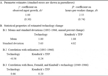
In part A of Table 1, I give the estimated coefficients on observed input growth and hours-per-worker change. Both are statistically significant. The coefficient on observed input growth, γ v , is 1.00. Since omitting hours-per-worker growth raised the estimate to 1.82 (not shown in the table), correcting for variable utilization makes increasing returns (suggested by high γ v if any) much less plausible. Basu, Fernald, and Kimball (Reference Basu, Clarida, Frankel, Giavazzi and West2006) show a similar finding for the post-WWII economy.
PARAMETER ESTIMATES AND PROPERTIES OF ESTIMATED TECHNOLOGY CHANGE

Notes:
Standard errors are heteroskedasticity- and autocorrelation-robust (calculated with RATS command of ROBUSTERRORS, LAGS=3, and LWINDOW=NEWEYWEST). Mean technology growth is calculated with residuals from the regression, plus a constant term.
Sources:
See the text.
Part B documents some statistical properties of this article's technology series, comparing with Kendrick's (Reference Kendrick1961, Reference Kendrick1973) TFP. Perhaps surprising, the standard deviation of my series is larger than Kendrick's, despite the adjustments for varying input utilization. This comes from the negative correlation of technology change with utilization at the aggregate level, which reduces the variance of TFP.Footnote 14 Indeed, as shown in the next row, my technology series has a negative correlation of –0.56 with hours-per-worker growth as a proxy for utilization, while Kendrick's (Reference Kendrick1961, Reference Kendrick1973) TFP series has a positive correlation of 0.24. Such negative correlation is also found by Basu, Fernald, and Kimball (Reference Basu, Clarida, Frankel, Giavazzi and West2006) for the post-WWII period and suggests that this article's adjustments of pre-WWII technology series for non-technology factors are effective. The final row shows more clearly the effectiveness of the adjustments. In the overlapping sample period of 1949–1966, my technology series has a correlation of 0.66 with Basu, Fernald, and Kimball's (Reference Basu, Clarida, Frankel, Giavazzi and West2006) series, while Kendrick's (Reference Kendrick1961, Reference Kendrick1973) TFP series has an insignificant correlation at 0.20.
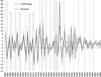
In Figure 1, I plot both this article's technology growth, which is measured by the residual series plus a constant term from the regression, and Kendrick's (Reference Kendrick1961, Reference Kendrick1973) TFP growth.Footnote 15 The figure shows large and persistent differences between the two series in the midst of the Great Depression contraction (1930–1932) and in an expansion phase following the start of WWII (1939). The differences come from adjustments for large fluctuations in utilization in those periods.
TECHNOLOGY CHANGE AND KENDRICK'S TFP GROWTH

Technology Change during the Great Depression
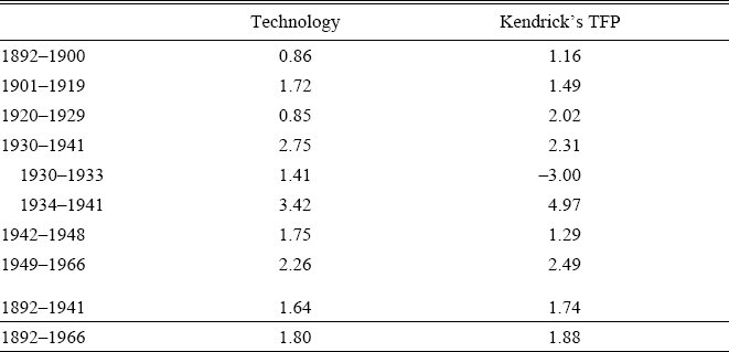
Table 2 displays the average technology growth rates, again with Kendrick's (Reference Kendrick1961, Reference Kendrick1973) TFP growth rates. The cut-off of each period between 1901 and 1948 follows Field (Reference Field2003, Reference Field2006, Reference Field2012), with the exception of subperiods in the 1940s, which he does not study.
AVERAGE ANNUAL TECHNOLOGY GROWTH AND TFP GROWTH

Notes:
Percent. Technology growth is calculated with residuals from the regression, plus a constant term.
Notes:
See the text.
Kendrick's (Reference Kendrick1961, Reference Kendrick1973) TFP recorded a historically large drop of –3 percent per year in the period 1930–1933. Such technology regress indicated by standard TFP series explains the large fall in output from 1929 to 1933 in Cole and Ohanian (Reference Cole and Ohanian1999) and Kehoe and Prescott's (Reference Kehoe and Prescott2008) standard neoclassical growth model. In contrast, my measure of technology shows that technology improvements continued at the pace of 1.41 percent per year over the same time period and it is difficult to attribute the cause of the Great Depression to technology regress.
In the recovery period 1934–1941, technology improvements accelerated to 3.42 percent per year. As a result, the average pace of technology improvements over the whole Great Depression period was 2.75 percent per year and higher than in any comparable periods in 1892–1966. This result supports Field's (Reference Field2003, Reference Field2006, Reference Field2012) argument that the period 1929–1941 was most technologically progressive in the U.S. economic history.
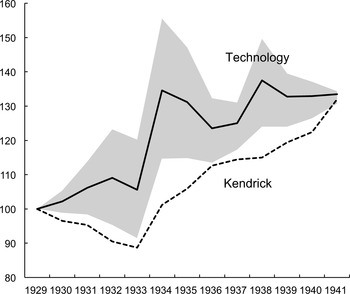
Figure 2 plots my technology series and Kendrick's TFP series during the Great Depression. While Kendrick's TFP declined by 12 percent between 1929 and 1933, the level of technology continued to increase between 1929 and 1932 before dropping in 1933, with a cumulative increase between 1929 and 1933 of 5.6 percent. The difference between the two series is statistically significant. Because the estimated coefficient on observed input growth, γ v , is 1.00, equation (4) implies that this difference is almost fully attributable to input utilization variations (multiplied by the coefficient β v , which reflects other adjustments as seen in the Online Appendix). Even at the lower bound of the confidence interval of technology series, falls in the first two years of the Great Depression are small. It appears unlikely, therefore, that technology regress triggered the downturn.
TECHNOLOGY AND KENDRICK'S TFP DURING THE GREAT DEPRESSION

In contrast, technology improvements accelerated in 1934 and are likely to have contributed to the recovery. Field (Reference Field2003, Reference Field2006, Reference Field2012) reviews a variety of microeconomic case studies and argues that the technical advances that occurred across the U.S. economy during the Great Depression era were successfully exploited in later periods, implying that the technology improvements had permanent effects on output. More subtle are the effects in the short run. The theoretical prediction varies depending on model specification, as summarized in Basu, Fernald, and Kimball (Reference Basu, Clarida, Frankel, Giavazzi and West2006). On the one hand, standard parameterizations of frictionless RBC models, as in Cole and Ohanian (Reference Cole and Ohanian1999) and Kehoe and Prescott (Reference Kehoe and Prescott2008), predict immediate increases in inputs and output in response to the technology improvements. On the other hand, with real inflexibilities due to habit persistence and investment adjustment costs, inputs fall and output changes little on impact because the expansion of demand is slow. Sticky price models without the Taylor rule predict the same: unchanged real balances resulting from the combination of unchanged money supply and sticky prices keep aggregate demand unchanged initially.Footnote 16 In a later section, I empirically study the short-run effects of a technology shock in the pre-WWII period using my technology series in a VAR model.
Robustness to Alternative Output Data
Nathan Balke and Robert Gordon (Reference Balke and Gordon1989) argue that the quality of Kendrick's (Reference Kendrick1961) gross national product (GNP) data is low especially for the period before 1909 and construct a new pre-WWII GNP series using unexploited data for non-commodity output and consumer prices. I now check the robustness of the baseline results by reflecting Balke and Gordon's (Reference Balke and Gordon1989) adjustments in Kendrick's (Reference Kendrick1961) private nonfarm output series and re-estimating equation (2) with the adjusted output series.Footnote 17
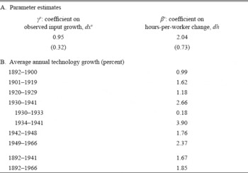
The upper part of Table 3 shows the results from the estimation. The estimated coefficient on observed input growth is 0.95 and similar to the baseline estimate of 1.00 shown in Table 1. The coefficient on hours-per-worker growth remains statistically significant. The lower part of Table 3 shows average technology growth calculated with the re-estimated parameters. Technology growth was 0.18 percent per year in the period 1929–1933 and 3.90 percent per year in the period 1934–1941. Hence, the baseline results of no technology regress in the downturn phase of the Great Depression and rapid technology improvements in the recovery phase are robust to the alternative measurement of output.Footnote 18
ADJUSTING PRE-1909 OUTPUT DATA

Notes:
Standard errors are heteroskedasticity- and autocorrelation-robust (calculated with RATS command of ROBUSTERRORS, LAGS=3, and LWINDOW=NEWEYWEST). Technology growth is calculated with residuals from the regression, plus a constant term.
Sources:
See the text.
COMPARISON WITH EXISTING STUDIES
This article is closely related to the work of Inklaar, de Jong, and Gouma (Reference Inklaar, de Jong and Gouma2011) and Ohanian (Reference Ohanian2001), who also study technology change during the Great Depression. Inklaar, de Jong, and Gouma (Reference Inklaar, de Jong and Gouma2011) propose their own approach to estimating pre-WWII technology change, while Ohanian (Reference Ohanian2001) examines several non-technology factors potentially driving TFP change during the Great Depression. This section compares my approach and results to those in these previous articles.
Inklaar, de Jong, and Gouma's (Reference Inklaar, de Jong and Gouma2011) Approach to Estimating Technology Change
Inklaar, de Jong, and Gouma (Reference Inklaar, de Jong and Gouma2011) estimate technology change in manufacturing industries in the period 1919–1939 with biennial data. The important difference between Inklaar, de Jong, and Gouma (Reference Inklaar, de Jong and Gouma2011) and this article is that this article estimates technology change for the private nonfarm economy while they do so only for the manufacturing sector, which accounted for around 20 percent of national income in the 1920s and 1930s.Footnote 19 Methodologically, contrary to their assertion that they follow Basu, Fernald, and Kimball (Reference Basu, Clarida, Frankel, Giavazzi and West2006) and Basu (Reference Basu1996), they do not do so in some important aspects and the reliability of their technology measure is unclear.
An essential part in Basu, Fernald, and Kimball's (Reference Basu, Clarida, Frankel, Giavazzi and West2006) approach is to use hours worked per worker as a proxy for unobserved input utilization, based on their finding of a theoretical foundation for a proportional relationship between the two variables. Inklaar, de Jong, and Gouma (Reference Inklaar, de Jong and Gouma2011) do not follow them and use intermediate inputs as a proxy for unobserved input utilization, asserting that such treatment is in the spirit of Basu (Reference Basu1996). However, Basu (Reference Basu1996) uses intermediate inputs as a proxy for total value added, which is produced by observed inputs as well as unobserved input utilization. Thus, Inklaar, de Jong, and Gouma (Reference Inklaar, de Jong and Gouma2011) do not follow even Basu (Reference Basu1996). Moreover, their linking unobserved input utilization directly with intermediate inputs is not theoretically valid.Footnote 20 Another difference between Basu, Fernald, and Kimball (Reference Basu, Clarida, Frankel, Giavazzi and West2006) and Inklaar, de Jong, and Gouma (Reference Inklaar, de Jong and Gouma2011) is that Basu, Fernald, and Kimball (Reference Basu, Clarida, Frankel, Giavazzi and West2006) estimate industry-level regression equations and aggregate industry technology changes by industry shares in total value added in order to adjust for reallocation effects, while Inklaar, de Jong, and Gouma (Reference Inklaar, de Jong and Gouma2011) do not do so. Instead, Inklaar, de Jong, and Gouma (Reference Inklaar, de Jong and Gouma2011) estimate a production function with panel industry data. Problematically, they calculate their technology measure as differences between total value added growth and the cost-share-weighted sum of industry input growth, the latter of which is multiplied by their increasing-returns-to-scale estimate. The increasing-returns-to-scale estimate comes from the panel data regression that gives an equal weight to each industry and does not reflect differences across industries in the share in total value added.
In addition, contrary to this article's decision, Inklaar, de Jong, and Gouma (Reference Inklaar, de Jong and Gouma2011) use oil price changes as one of their instruments, justifying their choice by the fact of the frequent use of the oil price changes as an instrument for post-WWII data. However, their results from a first stage regression are similar to what I found: the parameter estimate on the oil price changes is positive and indicates that the pre-WWII oil price change did not work as the negative supply shock.Footnote 21 Given the difference in the property of the oil price shock between the pre- and post-WWII periods, the validity of their choice of the oil price changes as the instrument is unclear.
Despite the small sector coverage and some potential methodological problems, Inklaar, de Jong, and Gouma (Reference Inklaar, de Jong and Gouma2011) reach the same conclusion as found here: technology regress is not likely to have triggered the Great Depression. This may, however, be partly due to coincidence. In the Online Appendix, I reproduce their technology series and show that their series and my series are different in the sign of change in many periods.Footnote 22
Ohanian's (Reference Ohanian2001) Analysis of Productivity Falls during the Great Depression
Ohanian (Reference Ohanian2001) and this article investigate the source of productivity falls during the downturn phase of the Great Depression (1929–1933) from a similar viewpoint. Ohanian (Reference Ohanian2001) concludes that the contribution of non-technology factors to an 18-percent decrease in Kendrick's (Reference Kendrick1961) TFP (of the national economy) is only 5-percentage points, which consist of 3-percentage point contribution of increasing returns to scale and 2-percentage point contribution of the mismeasurement of factor inputs.
The main source of differences in the evaluation between the two articles is the evaluation of varying input utilization. One possible reason for Ohanian's (Reference Ohanian2001) undervaluation is his non-adjustment for labor efforts, which may have had a relatively large contribution to the TFP decrease, reflecting labor shares. A second possibility is Ohanian's (Reference Ohanian2001) rough evaluation of the negative impact of declines in capital utilization, which is based on Timothy Bresnahan and Daniel Raff's (Reference Bresnahan and Raff1991) report that the number of active manufacturing establishments fell one-third between 1929 and 1933.Footnote 23 In contrast, I econometrically control my technology series for varying input utilization by following Basu, Fernald, and Kimball's (Reference Basu, Clarida, Frankel, Giavazzi and West2006) approach.
DYNAMIC RESPONSES TO TECHNOLOGY IMPROVEMENTS
So far I have evaluated Cole and Ohanian (Reference Cole and Ohanian1999) and Kehoe and Prescott's (Reference Kehoe and Prescott2008) technology-driven Great Depression hypothesis from the viewpoint of the adequacy of their productivity measurement and shown that their measure is lacking. Another approach is to evaluate the adequacy of their use of the standard RBC models in studying the Great Depression. As discussed above, the standard RBC model predicts immediate increases in output and inputs in response to the technology improvements, while sticky price models and models with real inflexibilities do not. If the economy was described by the latter models, technology change would be less able to trigger the downturn and the recovery. Indeed, Galí (Reference Galí1999) and Basu, Fernald, and Kimball (Reference Basu, Clarida, Frankel, Giavazzi and West2006) find in post-WWII data that hours worked decrease in response to a positive technology shock and argue that this finding is inconsistent with the standard RBC model's prediction. I apply a similar exercise to pre-WW II data.
I now estimate a near-VAR model, where the first equation regresses the log level of my technology series, z t , on z t –1 and the second equation regresses the log level of a variable of interest, j t , on j t –1, z t , and z t–1 . The log level of technology is the cumulated growth rate of technology. The lag selection criteria, AIC, BIC, or both, favor one lag in all regressions. I choose 1914–1941 for the sample period so as to have the results unaffected by the change in the institutional setting of monetary policy with the start of formal operation of the Federal Reserve in 1914.
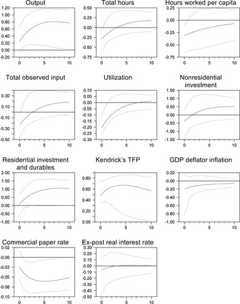
Figure 3 displays impulse responses to 1-percent shock to the technology series.Footnote 24 What I find is that the response of output is not statistically significant on impact, and then becomes larger and statistically significant. Hours worked, hours worked per capita, total observed input, and utilization all fall on impact and then increase through the ten-year horizon. The impact responses of output and inputs are very similar to the post-WWII responses found by Basu, Fernald, and Kimball (Reference Basu, Clarida, Frankel, Giavazzi and West2006). Thus, the standard RBC model, where output and inputs increase in response to technology improvements, is consistent neither with post-WWII short-run business cycle fluctuations nor with pre-WWII ones. The initial response of non-residential fixed investment and that of residential investment and durable consumption are statistically insignificant and might be explained by a real inflexibility model. The commercial paper rate, which is an available historical series of the short-term interest rate, falls significantly, but the real rate measured with one-period ahead GDP deflator inflation does not fall significantly. Monetary accommodation in response to a positive technology shock is not found in this article's pre-WWII data.
IMPULSE RESPONSES TO A POSITIVE TECHNOLOGY SHOCK

The results for output and inputs suggest that the use of the standard RBC model is not adequate for studying the role of technology change in pre-WWII business cycles. The insignificant response of output on impact may suggest that the technology improvements during the Great Depression, as indicated by this article's technology series, contributed to the recovery with a lag. Given that output began to increase in 1933, it may be more likely that the recovery was triggered by non-technology shocks such as inflation expectation shocks advocated by Peter Temin and Barrie Wigmore (Reference Temin and Wigmore1990) and Gauti Eggertsson (Reference Eggertsson2008, Reference Eggertsson2012).
CONCLUSION
Standard productivity measures indicate large fluctuations in technology during the Great Depression. This article's new measure of technology change, controlled for aggregation effects, varying input utilization, non-constant returns, and imperfect competition, does not indicate technology regress such that could trigger the downturn.Footnote 25 In contrast, rapid technology improvements appear to have contributed to the recovery, maybe with a lag. Average technology growth over the whole Great Depression period was higher than in any other pre-WWII decades.
This article's results suggest the importance of the purified TFP measure in studying the role of technology change in business cycles. Temin (Reference Temin2008, Reference Temin2009) criticizes Cole and Ohanian (Reference Cole and Ohanian1999) and Kehoe and Prescott's (Reference Kehoe and Prescott2008) exercises for providing little guidance in answering why productivity fell so sharply. Such debate loses importance, since this article's new measure, on average, suggests almost no technology regress during the Great Depression. In contrast, this article's finding for the recovery supports the idea that technology improvements contributed to the recovery and the quantitative importance of those is worth investigating. Potentially it is important to take into account that the U.S. economy faced the zero nominal interest rate bound in the recovery phase of the Great Depression (Eggertsson Reference Eggertsson2008, Reference Eggertsson2012). The effects of a permanent rise in the technology level can become large in such economic environment, because interest rates do not rise. A recently growing literature on how macroeconomic shocks affect the economy at the zero nominal interest rate might shed a new light on the role of technology improvements in the recovery period of the Great Depression.Footnote 26
Appendix: Data Sources
Output, Total Hours Worked, and Capital Stock
Data for output, hours, and nonresidential capital stock in the private nonfarm sector are from Kendrick (Reference Kendrick1961, Reference Kendrick1973). Data from the former is linked to ones from the latter in 1948.
Aggregate Hours Per Worker
Data for aggregate hours per worker as a proxy for utilization are constructed by aggregating data for hours per worker for mining, manufacturing, transportation, and the other sectors. Data for hours and employment are from Kendrick (Reference Kendrick1961, Reference Kendrick1973). Data for the other sectors are computed by subtracting data for the three industries from data for the whole private nonfarm sector. The aggregation uses industry shares in national income, reported in the U.S. Department of Commerce (1958) for the period 1929–1957. The 1929 share is used for the period 1893–1929, the average share of 1930–1937 is used for the 1930–1937 period, the average share of 1938–1947 is used for the 1938–1947 period, and the 1957 share is used for the 1948–1966 period. Following Basu, Fernald, and Kimball (Reference Basu, Clarida, Frankel, Giavazzi and West2006), I detrend log hours-per-worker series with Laurence Christiano and Terry Fitzgerald's (Reference Christiano and Fitzgerald2003) band pass filter to remove trend and make the series have zero mean. I drop frequency components of 50 years and more. The parameter estimates are robust to using Hodrick-Prescott filter or first differences for the detrending.
Gold Production
Data for gold production are from Christopher Schmitz (Reference Schmitz1979).
Hours Worked Per Capita
Data for hours worked for the private nonfarm sector, which are used for calculating hours worked per capita to study the impulse response, are same as explained above. Data for hours worked for the total economy, which are used for calculating hours worked per capita to estimate permanent non-technology shocks, are constructed by splicing data published by the Bureau of Economic Analysis (BEA) for the period from 1948 to Kendrick's (Reference Kendrick1961) data. Population series is obtained from the Council of Economic Advisors (2010) for the post-1940 period. This series includes resident population aged 16 and over and armed forces overseas. This series is spliced to the series of resident population aged 15 and over obtained from the U.S. Census Bureau (2010) for the period 1900–1939. The number of armed forces overseas during WWI from the U.S. Department of Commerce (1975) is added to the data for 1918. The resultant series is spliced to series of total resident population from the U.S. Department of Commerce (1975) for the period 1889–1900.
Labor Productivity
Output series for numerator is constructed by splicing data for real GDP published by the BEA for the period from 1929 to Balke and Gordon's (Reference Balke and Gordon1989) data for real GNP. Data for hours worked in the total economy for denominator are same as previously explained.
Nominal Investment-Output Ratio
The nominal investment-output ratio series from 1901 is calculated by dividing the BEA's series of investment in private and government nonresidential fixed assets with the BEA's GDP series, which is extended back to 1901 by using Balke and Gordon's (Reference Balke and Gordon1989) nominal GNP series. I calculate the nominal investment-output ratio series in the period 1889–1909 mainly by using Robert Gallman's annual national product series from Paul Rhode (Reference Rhode2002). Rhode (Reference Rhode2002) states that “Gallman's number are among the best we have for the nineteenth century,” though Gallman's data were not constructed for analysis as annual series. The investment series is Gallman's series of the capital formation in manufactured producers' durables plus Gallman's gross new construction series minus the private nonfarm residential building series from the U.S. Department of Commerce (1975). The output series is the sum of Gallman's national product and inventory change series minus Gallman's series of changes in foreign claims. The ratio of the two series is spliced to the nominal investment-output ratio series from 1901 by using the 1901–1909 average of the latter relative to that of the former.
Nonresidential Investment, Residential Investment, and Consumer Durable Goods
Data for those are published by the BEA. The series for residential investment and consumer durable goods are aggregated by using the chain-type Fisher formula.
GDP Deflator
BEA's GDP deflator series for the period from 1929 is spliced to Balke and Gordon's (1989) GNP deflator series.
Commercial Paper Rates
Data for commercial paper rates are from NBER Macroeconomy Database.