FORECASTING PRESIDENTIAL ELECTIONS IN THE UNITED STATES

In “The State of Presidential Election Forecasting,” R.J. Jones (Reference Jones2008) provides an exhaustive review of 13 methods that have been previously used to predict US presidential elections. According to Michael Lewis-Beck (Reference Lewis-Beck2005), unlike others, only statistical estimation (forecasting) methods using economic and sociopolitical data are based on a real theory of voting.

Sigelman (Reference Sigelman1979), Lewis-Beck and Rice (Reference Lewis-Beck and Rice1982), Rosenstone (Reference Rosenstone1983), and Lewis-Beck and Rice (Reference Lewis-Beck and Rice1984) built the first statistical political economy models aimed at forecasting US elections. Among these, Rosenstone's pooling model, whose unit of study is the state, is exceptional. Following Rosenstone, two more pooling models were built: Holbrook's in 1991 and Campbell's in 1992. However, state-based models are still neglected; in the last 2008 Pollyvote survey, aggregated models were still dominant.

Our political economy model (PEM) is part of this state-based “family” but adds partisan dynamics at the state level, similar to the first political economy pooled time series models built for the 2002 French presidential election (Jérôme and Jérôme-Speziari Reference Jérôme and Jérôme-Speziari2001; Jérôme, Jérôme-Speziari, and Lewis-Beck Reference Jérôme, Jérôme-Speziari and Lewis-Beck2003).

Our PEM uses data for subnational units and then aggregates these subnational predictions to create an overall prediction. Using subnational data, our forecasting approach differs from all other models in the US forecasting literature (exceptions are previously mentioned). Our approach has the potential to substantially improve predictive accuracy insofar as local context matters for shaping beliefs about the economy and past performance of political actors.

First, we start with a search for the most significant explanatory variables to be included in our model. Next, we estimate voting patterns at the state level; then we switch to aggregate state-by-state predictions in terms of Electoral College vote share to predict the winner of the 2012 US presidential election.

WHY TAKE INTO ACCOUNT POLITICAL AND ECONOMIC DATA AT THE STATE LEVEL?

Pooling data obviously helps increase the number of observations in the dataset as well as the degrees of freedom; thus, we can expect the model to perform better. A larger number of observations also guarantees a minimization of biases due to aggregation effects. In addition, we use the so-called saving properties of aggregation so errors could be balanced. Pooling also allows for research into the “dynamics of change” (Baltagli Reference Baltagli1995). It also allows us to discern and to measure effects that are difficult to identify when either purely cross-sectional or purely longitudinal methods are used in isolation from each other. Finally, this approach allows us to come closer to studying behavior on the individual level.

In the United States, voting behavior has a territorial component. Because the US presidential election is normally decided by the Electoral College vote, there is a journalistic emphasis on studying the expected voting behavior of the “swing states.” American politician Tip O'Neill used to say, “All politics is local.” If local economic and social conditions, affect voters' electoral choices in a given geographic area, then we can improve our predictive accuracy at the national level by using pooled time series voting models that make use of state and regional data.

Sometimes long-term consistencies exist in voting behavior in particular geographic regions, but these are rarely immutable. Furthermore, local effects, like national effects, are triggered by factors such as changes in economic conditions, and, in the extreme, changes in local economic conditions can lead to outward or inward migration (Tiebout Reference Tiebout1956). Some states are stable in their ideology, whereas others are very unstable. Given these state-by-state idiosyncrasies, our vote function must reflect the evolution of “partisan domination” through time and space. To achieve this, we built two partisan representation indexes reflecting states' partisan particularities. For this purpose, we distinguish between the entire period under study (1952–2008) and the period 1980–2008 when significant partisan changes occurred in US politics.

From 1952 to 2008, Republicans were dominant in 12 out of 50 states (plus Washington, DC) (Alaska, Arizona, Idaho, Indiana, Kansas, Montana, Nebraska, North Dakota, Oklahoma, South Dakota, Virgina, and Wyoming); this means that Republicans have a long-term electoral base of 72 electoral votes (EVs), or 13.4% of the total EVs. If we perform the exact same calculation for Democrats,Footnote ² we find a long-term electoral base of 43 EVs, or 8% of the total EV (Hawaii, Maryland, Massachusetts, Minnesota, Rhode Island, and Washington, DC). These unassailable states are considered to be electoral strongholds for each party.

However, some states are “swing states” or states that realign over time (see Merrill, Grofman, and Brunell Reference Merrill, Grofman and Brunell2008), such that both Democrats and Republicans profit from what we call a “new domination” since 1980. For Democrats, this potential new domination can be seen in California, Connecticut, Delaware, Iowa, Illinois, Maine, Michigan, New Jersey, New York, Oregon, Pennsylvania, Vermont, Washington, and Wisconsin, which translates into 213 EVs, or 39% of the total EVs. For Republicans, their potential new domination may appear in Alabama, Arizona, Georgia, Kentucky, Louisiana, Mississippi, Missouri, North Carolina, South Carolina, Tennessee, Texas, and Utah, which amounts to 137 EVs, or 25.5% of the total EVs. We must highlight that the Republicans' gains are mostly in the southern states (except Missouri and Utah), where they have captured “southern Democrats.” Finally, six states remain without strong partisan domination, and they represent 48 EVs, or 9% of the total EVs.

A STATE-BY-STATE POLITICAL ECONOMY FORECASTING MODEL FOR US PRESIDENTIAL ELECTIONS

Models built on vote functions are based on a theory of governmental responsibility (Key Reference Key1966). Vote functions offer an explicative model of voters' choices and preferences and provide a model of votes for an incumbent based on political and economic performances. Vote functions need to include “good” political and economic variables side-by-side to gain stability (Nannestad and Paldam Reference Nannestad and Paldam1994). In addition, pure economic vote functions (see Fair Reference Fair1978) are regularly underspecified and lead to significant errors when these are used in electoral forecasting. Thus, Rosenstone (Reference Rosenstone1983, 45) argues that an aggregated voting model that keeps only one of the above-mentioned possibilities could not explain why citizens change their vote from one election to the other.

Next, we include the structural model from which we compute the ordinary least squares (OLS) regression estimates, along with the operationalization of the variables from 1980–2008 in the 50 American states plus Washington, DC (N = 408):

$$ \displaylines{ {\rm INCV}_{i,t} = C + \Delta {\rm UL}_{i,t - n} + {\rm PJA}_{t - n} + {\rm LPD}_{i,t - n} \cr + {\rm Politics and Institutions}_{i,t - n} \cr + {\rm President's Local Strongholds}_{i,t - n} \cr + {\rm Local Electoral Peculiarities}_{i,t - n} + {\rm Error} \cr} $$

The dependent variable INCV_i,t measures the vote share in the ith state (i = 1,…,51) and for the tth time period (t = 1980, 1984,…,2008) going to the ruling political party. The incumbent president was a Democrat in 1980, 1996, and 2000 and was a Republican in 1984, 1988, 1992, 2004, and 2008.

For the explanatory variables, the first variable (ΔU) is the change in the local (i.e., state-level) unemployment rate from the month after the president was elected to the month prior to the next presidential election. A positive change in state unemployment should cost the incumbent a portion of his vote share. The second variable is the Gallup President's Job Approval (PJA), at a national level, six months before the election. For the outgoing majority candidate, the higher the president's popularity is, the higher the electoral premium. However, the impact of popularity should not be the same and depends on whether the incumbent is seeking a second term or not. Thus, PJA2 is the president's popularity when he is seeking a second term (and 0 otherwise). PJA0 is the President's Job Approval when the incumbent is not running for a second term. Following the above discussion, the third variable, Local Partisan Domination (LPD), takes into account the characteristics of the partisan cycle in each state. LPD is divided into two local partisan domination variables, one named LPD5208 to code states having significant partisan domination since 1952 and another one called LPD8008, or “new domination” since 1980, which includes recent southern Republican strongholds. More precisely, for each state during the 1952–2008 period, LPD5208 gives the rate of success for each party when this rate exceeded 85%Footnote ³ for the Republicans and 61% for the Democrats (this variable takes a 0 value otherwise). When the ideology of the state is the same as the incumbent, it carries a “+” sign; otherwise, it carries a “−” sign. This means that an incumbent will be rewarded by states that are ideologically similar and punished by states that are ideologically dissimilar. The LPD8008 variable was constructed in the same way, except that the rate of success is calculated for 1980–2008.

Some other explanatory variables used to build the econometric model deal with politics and institutions (i.e., the electoral weight of independent candidates), the president's electoral strongholds (i.e., measuring home state advantage), and local electoral peculiarities such as scores usually deviating from the standard (Democrats in Washington, DC, for instance). The specification of these variables whose estimated coefficients are not used to forecast the 2012 election is described in the appendix.

EMPIRICAL RESULTS

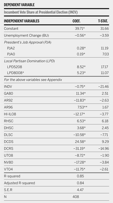
Overall, if one focuses on the main variables, the aforementioned US presidential vote model gives good statistical results (see table 1). This model explains 85% of the variance, and all the coefficients are statistically significant (t-ratios at 0.05, two-tailed) except AR96 t-ratio at 0.10.

Table 1

2012 US Presidential Election Political Economy Model Pooled Time Series 50 States and DC (1980–2008)

^a Including Southern Republican new Strongholds

* Significance at a 1% level (two-tails)

** Significance at a 5% level (two-tails)

The standard error of regression (SER) is 4.47. This means that each estimated score in each state has to be interpreted with a ±4.47 error margin. Furthermore, all of the coefficients for the explanatory variables in the presidential vote function (for incumbents) have the expected signs.

Among the variables kept for forecasting, we underline the fact that the constant provides an estimate for the incumbent's electoral base of 39.71% of the long-run vote share. On average, a one-point rise in the unemployment rate costs the incumbent 0.56% of the votes in a given state. In case of a second term, a 50% approval score yields 14% more votes. However, in the case of new candidate (from the incumbent's same party), a popularity score of 50% for the president yields only 9.50% more votes.

The outgoing majority on average gains 8.52%, depending on the party's historical strength in a particular state (LPD5208). Conversely, in such strongholds, the opposition candidate suffers a 8.52% electoral disadvantage. In what we call “new partisan domination” states (LPD8008) measured between 1980 and 2008, the outgoing majority on average gains 5.23% in their strongholds, while the opposition candidate suffers a 5.23% electoral loss.

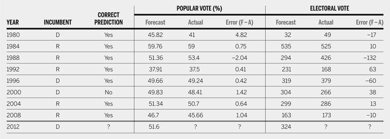
To see if we can trust this model, we can test it through electoral “backcasting” for previous elections. The observed and forecasted aggregated electoral results for the incumbent are displayed in table 2. Except for 2000, both electoral and popular votes are adequately predicted and the winner is correctly determined.

Table 2

Ex-Post Forecasts Accuracy

FORECASTING, SCENARIOS, AND DISCUSSION

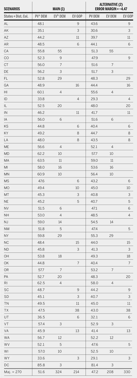
The 2012 preelection values have been plugged into the model to predict the popular votes in each state. Table 3 shows the incumbent state-by-state vote share forecasts according to two scenarios. The first one, our main scenario (column 1), is based on economic (change in unemployment) and political (Obama's approval job rate) factors available in June 2012. Our second scenario (column 2) hypothesizes that Barack Obama may be threatened by an “anti-Obama” referendum similar to what befell Nicolas Sarkozy in France. This specific case aims at measuring indirectly what would happen if concerns not accounted for in our model, such as the unpopularity of health-care reform or a “racial cost” (see Lewis-Beck, Tien, and Nadeau Reference Lewis-Beck, Tien and Nadeau2010), were to have a deep and negative impact on Obama's vote share. To simulate this, we have imputed a −4.47 percentage points error margin to the incumbent's forecasted votes issued from our main scenario.

Table 3

State-by-State Political Economy Model 2012 Forecast (Sept. 2012) Popular Votes and Electoral Votes for Democrats

^a PV: Popular Vote; ^bEV: Electoral Vote

With regard to the main scenario, the forecasting model (launched to predict 2004 and 2008 elections) gives an absolute majority for the Democrats with 51.6% of the popular votes (−1.2% compared with 2008) and 324 EVs (−39 compared with 2008). This simulation shows a slight increase in popular vote (+0.4) from our previous forecast calculated in August 2011. However, one can observe a near status quo regarding the electoral vote.

Thus, if the elections were held in September 2012, the Democrats would obtain a majority of the popular votes in 27 states (−2 compared with 2008). According to the forecast, the Republicans would regain two of its southern strongholds that it lost in 2008: North Carolina (15 EVs) and Virginia (13 EVs). To this, we can also add a victory in Indiana (11 EVs). However, Republicans would lose West Virginia (5 EVs).

How do we explain this result? Basically, after peaking at 10% in October 2009, the unemployment rate has been decreasing and has stabilized at around 8.2% in May and June (compared to 7.8% when Obama took office). This evolution enables the Democrats to resist in most of their historical and “new” strongholds. In addition, the incumbent president's credibility is still rather high (46.4% were satisfied with his performance in March 2012, Gallup USA Today), compared with George W. Bush's approval rating in March 2007 (when 33% were satisfied). Translating this into votes, this means on average an electoral gain of 3.9Footnote ⁴ points per state compared with George W. Bush's situation at the same time.

However, if we uniformly apply a −4.47 point error margin to Democrats in each state to measure factors not accounted for in our explanatory variables, we find that Mitt Romney could pull off a backdoor victory in the 2012 election with 330 EVs and 52.8% of the vote share. First, this result shows that Obama's lead is rather fragile if an “anything but Obama” strategy dominates. Second, this simulation shows that nine states, Colorado, Florida, Illinois, Nevada, New Hampshire, New Mexico, Ohio, Pennsylvania, and West Virginia, could be decisive. Among them, four states (Florida, Illinois, Ohio, and Pennsylvania) account for 87 EVs.

If the likelihood of an “anti-Obama” referendum turns out to be smaller than expected, is there a baseline in terms of popularity and unemployment to guarantee a second term for the incumbent in November? Ceteris paribus, according to our calculations, if the unemployment rate exceeds 9.4% in September on the national level (e.g., a + 1.2 point change in unemployment on average) and if Barack Obama's job approval falls to 39%, then Mitt Romney would mathematically win 274 EVs and 51.1% of the popular vote. Moreover, the Republicans would win Colorado, Illinois, Nevada, New Mexico, Pennsylvania, and West Virginia.

Now a question arises: with five months remaining until the next election, will the European debt crisis and weakening growth worldwide significantly change Barack Obama's chances of victory? Notwithstanding extenuating circumstances or external and unforeseen shocks, one can doubt it, and the Democrats should have a second term in the White House. However, as our state-by-state model shows, the Democrats will have to keep an eye on Florida, Illinois, Ohio, and Pennsylvania to maximize their chances of reelection.