Thirty States join in making next Tuesday their election day—a number unprecedented, save, of course, in Presidential years. … [They] now by law regularly hold their elections for State officers and Congressmen on the Tuesday next after the first Monday in November.
… [T]he advantages of uniformity are incontestable. The exaggerated and unreasonable influence of the September-voting States upon the October-voting States, and of these in turn upon the November-voting States, has for many years been notorious. It is, of course, absurd that elections in one part of the country, which may have turned on special causes, should influence all the rest of the Union.
… We see no good reason why it should not be not only almost but altogether uniform.Footnote 1
I. Introduction
“The first Tuesday after the first Monday in November”—by this simple rule, Americans organize 435 congressional election contests into one simultaneous collective event. Many—including not a few political scientists—treat this scheduling requirement as though it were an enduring feature of American political history, perhaps even one of the Framers' constitutional stipulations. In fact, the historical pattern is richer and more variegated. For much of the country's first hundred years, diversity, not uniformity, was a defining feature of the congressional election schedule. The non-synchronous character of this first American scheduling regime manifested itself in two especially critical ways. First, non-synchronicity within states separated congressional and presidential elections in time, creating a host of problems for political parties, from the challenges of multiple mobilization efforts, to the difficulties of ensuring a unified party vote across federal elections that could be separated by several months. Second, non-synchronicity across states in congressional elections meant that legislative races unfolded sequentially over time, exposing these predominantly local contests to distinctive interstate contagions—not unlike contemporary presidential primaries—with unexpected partisan showings in early state races helping to shape outcomes in subsequent state contests.
A brief description of the 1848 congressional elections will highlight the distinctiveness of this period and help motivate the discussion that follows. In point of fact, the 1848 electoral season actually extended a full fifteen months. Arkansas, Illinois, Iowa, and Missouri went first in the cycle, with elections scheduled for 7 August 1848. Louisiana and Mississippi closed the season with elections held on 5 November 1849, less than a month before the start of the new Congress.Footnote 2 In between these contests, elections in the remaining twenty-five states were scheduled on fourteen additional calendar dates.
In a campaign season so ordered in time, early elections were political laboratories of sorts, and their outcomes could easily influence party strategies in subsequent races. To continue our example, Whig congressional strategists in 1848 hoped to parlay popular support for their presidential candidate, the popular military general Zachary M. Taylor, into control of the House of Representatives. In early state races, Whig candidates emphasized nonpartisanship, issue avoidance, and the trumpeting of U.S. martial glory—a strategy smartly tailored to fit the qualities of the Whig presidential candidate. This strategy, however, was quickly adjudged a failure in state congressional races, neither attracting Democratic defectors nor energizing the Whig Party faithful. However with so much of the campaign season still to go, Whigs could discard this strategy; and they did, subsequently hammering away at local issues, sharpening party differences, “and condemning rather than courting Democrats.”Footnote 3
The dynamics of this elongated election season were more complicated still. In the course of a fifteen-month-long congressional cycle, different national and sectional issues could swirl in and out of state races as exogenous political shocks invaded the public sphere. Both slavery extension and war were hot button issues in 1848. Southern Whig candidates might be pressed by Democrats to defend more aggressively their region's “peculiar institution” or U.S. involvement in the 1846 Mexican-American War. Northern Whig contenders, on the other hand, might find it just as necessary to condemn that same war or sharpen their antislavery bona fides (especially in those districts where the Free Soil Party was running strong).
Finally, in a system where state politicians controlled the election calendar, the organization of the congressional season was bound to reflect their changing political needs. Consequently, the nineteenth-century congressional schedule was far from static. In fact, in 1848, critical new changes were already beginning to take shape. Over the next twelve years, the profound sectional polarity seizing the nation would insinuate itself into the basic structure of the congressional election season. Many northern states, first slowly, and then with greater frequency, would coalesce on the first Tuesday after the first Monday in November (hereafter 1T/1M) as the date on which to hold their elections to Congress. Southern states, on the other hand, would intensify their long-standing preference for odd-year congressional elections, typically scheduling them several months after the presidential season had concluded. Only in 1872 would Congress finally make the 1T/1M rule binding on all states, though it would still be a number of years before full compliance was actually accomplished.
In this article, I examine the impact of nineteenth-century election scheduling on party electoral performance. The institutional features of the nineteenth-century electoral calendar make them unique in American political history. My central focus is on the sequential structure of the congressional election season. This little-studied facet of American politics was endemic to House contests for the first seventy-five years of constitutional government. Because partisan competition to control the House of Representatives stretched over many months, these contests can fruitfully be studied in a manner similar to that employed by students of the modern presidential primary system.Footnote 4 In both, the welter of individual state laws governing election scheduling renders matters of timing—when state elections are held—and sequence—the distinctive interstate political effects generated by that temporal ordering—integral to the rhythms of the electoral season.
I will demonstrate that interstate “political contagion” was a distinctive feature of congressional elections between 1828 and 1874, an artifact of the era's temporally fragmented electoral calendar. Specifically, I will present both qualitative and quantitative evidence to support the claim that early party victories in state congressional races influenced the vote in subsequent state contests, and did so in a manner benefiting the previous party victor. I will also offer statistical evidence to suggest that while sequential presidential elections (1828–1844) never exhibited the same kind of political contagion manifested in the congressional sphere, an interstate contagion effect did find its way into non-federal contests, like the race for governor.
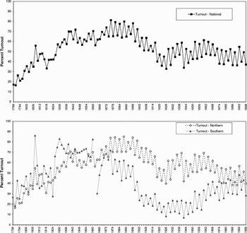
The formal synchronization of congressional elections on 1T/1M in the 1870s fundamentally altered the politics of congressional elections. In removing this sequentially-induced political dynamic from play, this new scheduling regime simultaneously coupled and uncoupled these local contests from supra-local political forces, exposing them with full force to coattail effects in presidential election years, while rendering them more insular affairs at midterm. In this fashion, the new national uniformity in federal election scheduling helped foster the now familiar rhythm of “surge and decline” in congressional elections, which also emerged between 1872 and 1876, and which remains today a hallmark of American congressional elections (see Figure 1).
The Presence of “Surge and Decline in Congressional Elections, 1788–1998.”

This article is organized into two parts. The first examines the trend toward 1T/1M in congressional election scheduling and briefly considers some of the historical forces driving change over time. Following this, I turn to the politics of sequential congressional elections between 1828 and 1874, focusing specifically on the inter-temporal properties distinctive to this era's scheduling regime. In particular, I present both anecdotal and systematic evidence for the presence of interstate political contagion in congressional elections. Statistical tests for contagion effects in sequential presidential and gubernatorial elections are also conducted. A conclusion follows.
II. TOWARD 1T/1M: HISTORICAL FORCES AND INSTITUTIONAL CHANGE
The electoral fragmentation characteristic of America's first scheduling regime was a natural expression of the Founding ethos of federalism and states' rights. Conversely, the movement toward 1T/1M in congressional elections, it seems, was intimately tied to the increasing nationalization of American politics over the course of the nineteenth century. That trend started in 1848, given initial impetus by the federal law of 23 January 1845 mandating 1T/1M in presidential elections. Political elites in Washington justified the 1845 law as an attack on a distinctive form of political corruption. Sequential presidential elections, it was argued, gave organized gangs of “repeaters” both motive and opportunity to ferry across interstate lines and cast multiple votes for their party's presidential candidate.Footnote 5 Interstate uniformity in election schedules removed this element from play, bringing with it a heightened confidence in the integrity of the presidential selection process. In the end, congressional elections were left outside the reach of the 1845 law, even though repeating (or “colonizing”) posed problems in these contests as well.Footnote 6 Still, individual sets of contiguous states remained free by law to synchronize their congressional elections voluntarily and thereby curb this special form of corruption.
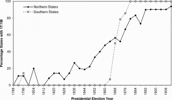
The 1845 presidential 1T/1M law provided a focal point around which future scheduling changes might coalesce, and is therefore an important first step in understanding the convergence on 1T/1M in congressional elections. Likewise, the problem of colonizing in state congressional races also provided a clear motive for change.Footnote 7 However, other striking patterns remain submerged in the standard corruption narrative. In particular, as Figure 2 shows, prior to the Civil War, the movement of congressional elections onto 1T/1M was exclusively a Northern phenomenon. While the reasons remain murky, it is clear that the synchronization of presidential and congressional elections on 1T/1M was attractive to Northern states but not so to Southern states—a pattern that invites questions regarding the role antislavery politics might have played in driving this bifurcated scheduling arrangement. Indeed, it was only in the aftermath of the Civil War and the Republican Party's Reconstruction efforts that Southern states would first come to adopt 1T/1M.Footnote 8 A second pattern worth noting is that the movement to 1T/1M in Northern congressional elections was gradual. In 1848, three years after the passage of the presidential law, only four Northern states—New York, New Jersey, Michigan, and Wisconsin—were employing the 1T/1M rule in congressional elections.Footnote 9 That number grew to six states in 1852, eight in 1856, and ten in 1860, expanding almost in tandem with the Northern antislavery movement.
Percentage of Northern and Southern States Scheduling 1T/1M Elections for Congress, 1788–1912.

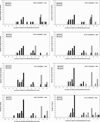
Figure 3 depicts graphically the deepening sectional polarity in antebellum election calendars. While within-section variation is always discernible, it is clear that a broad Northern preference for scheduling presidential-year congressional contests prior to the presidential contest was gradually replaced with synchronization on 1T/1M. On the other hand, a long-established Southern tradition of holding presidential-year congressional elections in the off-year, long after the national presidential contest had concluded, grew substantially more uniform, though the Southern calendar never coalesced around a single date as it did in the North. To date, I have found no direct evidence to suggest that sectional politicians coordinated their electoral calendars to advance shared interests, like those that coalesced around the slavery question. Nevertheless, it is hard to ignore the fact that congressional elections were riding presidential coattails in the North; in the South, on the other hand, wider effort was made to decouple and thus insulate congressional elections from the contagion of the presidential contest.
Sectional Polarization in Congressional Election Scheduling, 1832–1860.

In the end, whatever factors propelled the move toward uniformity in federal election scheduling, by 1872—the year Congress first mandated the 1T/1M rule in congressional elections—about half of all northern states and three-quarters of all southern states were already holding such contests. In that sense, the 1872 federal law simply ratified and extended a growing trend at the state level. However, additional momentum in support of scheduling uniformity was also conditioned, as the New York Times told its readers, by the “exaggerated and unreasonable influence” of early-voting states upon the later-voting states.”Footnote 10 Such considerations were raised explicitly in the course of the 1871 congressional debate to adopt the 1T/1M rule in congressional elections. Massachusetts Republican Benjamin Butler, who sponsored the amendment that became the 1872 1T/1M law, explicitly argued that the absence of a uniform election date gave some states (and some political parties) undue electoral advantages.
Unless we do fix some time at which, as a rule, Representatives shall be elected, it will be in the power of each state to fix upon a different day, and we may have a canvas going on all over the Union at different times. It gives some states undue advantage. It gives some parties undo advantage. … I agree that … the elections in Vermont and the elections in California in September … have a great influence on the other elections. I agree also that Indiana, Ohio, and Pennsylvania, by voting in October, have an influence. But what I contend is that that is an undue advantage, that it is a wrong.Footnote 11
Political corruption was a second consideration that fueled the national move to 1T/1M, though even this concern cannot be divorced fully from the electoral dynamics of interstate contagion. The widely known effects of early-state results on later-voting states fueled partisan efforts to ensure an appropriate outcome in the early states—sometimes by any means possible. As the New York Times again observed,
Few things … have done more to encourage bribery, fraudulent registry, repeating, and mob violence at the polling-booths than the want of uniform State election days. We do not now see quite so much eagerness as formerly in this respect. As has been said, several of the States which used to vote earlier in the year, disgusted with the hard experience of being made annual battle-grounds for the whole Union, have joined the November fold.Footnote 12
In the end, it is perhaps surprising that, in 1880, the South, which for so long had resisted the trend, came first into full compliance with the national 1T/1M law. Rogan Kersh suggests that in the new post-Reconstruction political order, quick Southern compliance was a symbolic gesture of national reunification.Footnote 13 Be that as it may, by 1888 the last populous Northern state had also come into the fold (Ohio), though Oregon, Vermont, and Maine continued to buck the trend: in the case of the first two states, noncompliance persisted until 1910 and 1914 respectively; in the case of the latter, compliance was not secured until 1960.Footnote 14
III. POLITICAL CONTAGION IN SEQUENTIAL CONGRESSIONAL ELECTIONS, 1828–1874
In this section, I offer additional historical material to support the claim that interstate “political contagion” was a well-understood phenomenon in nineteenth-century congressional elections. Contemporaneous observers regularly discussed the political implications of early-state election outcomes for later-state voting patterns. The sequential nature of these contests was held to inject a distinctive political current into the period's legislative races, one that favored the party that emerged victorious in early-state contests. Students of the modern sequential presidential primary system refer to this inter-temporal electoral dynamic as “momentum” or the “bandwagon effect.”Footnote 15 The structural similarity of these elongated congressional seasons suggests a similar role for interstate contagion in these temporally-unfolding House contests.
A Model of Contagion in Congressional Elections
What is political contagion? How is it created? How is it transmitted in sequential congressional elections? As used here, political contagion refers to an electoral stimulus of interstate origin. It is generated when an unexpected change in relative party performance in state i at time t-1 stimulates vote change in the same partisan direction in state k at time t. By “unexpected change,” I mean a departure from normal partisan voting patterns characteristic of a state's electoral politics. By “normal partisan voting patterns,” I mean some baseline expectation for current party performance predicated on knowledge of prior state-voting patterns.
The interstate transmission of political contagion in nineteenth-century congressional elections operated something as follows: Unexpected election outcomes in early-voting states—those outcomes adjudged significantly larger or smaller than conventional expectations—invited sustained post-election discussion, prognostication, and general ballyhoo by political professionals and other partisan elites in later-sequence states. Newspapers and other periodicals of the day were the central institutional transmission belts, connecting out-of-state election results to in-state voters soon to go to the polls. These journalists, mostly (though not always) partisan, fed their readers a heavy diet of election “horse-race analysis”—who was ahead, who was behind, who was coming up fast, and who was crossing the finish line first in recently concluded races. Suggestive of this is the following 1848 headline from one Whig newspaper, the Norwalk Huron Reflector:
OCTOBER ELECTIONS
Whig Victories in
OHIO
GEORGIA
FLORIDA
DELAWARE
MARYLAND
PENNSYLVANIA
A shout from the Alleghenies—the Whig
Avalanche in motion!Footnote 16
As Election Day approached, voters in later-voting states—especially those whom modern political science has termed “low-information voters”—consumed this horse-race information regarding the relative showing of the parties in previous state contests. This information, in conjunction with the strength of standing partisan attachments, helped form the basis for the congressional vote, with some subset of voters reassessing their partisan commitments in a manner favorable to the recently victorious party.
As the preceding paragraph indicates, I am suggesting an explicit affinity between nineteenth-century sequential congressional elections and our contemporary sequential presidential primary system. That said, there are important differences as well. A critical difference is the place that party holds in my analysis—both as an organization and as a voter attachment. In presidential primaries, individual candidates are the unit of interest. It is they who compete across a battery of states for bound delegates to the national party convention. In that setting, candidate party attachments wash out of the analytic frame. By contrast, my analysis requires parties to be both present and strong to make the analogy to modern presidential primary system work. It is the presence of organized parties that provides unit continuity across discrete contests involving otherwise unique candidates and contexts, allowing electoral performance in one state to impact electoral performance in another. In this regard, I would expect this model to perform less well—even assuming sequential scheduling—in contexts such as contemporary U.S. congressional elections, where career legislators with candidate-centered electoral organizations and assorted incumbency advantages make these contests much more heavily personalized affairs.Footnote 17 However, the model sketched here offers a decidedly more comfortable fit for the so-called “party period” of nineteenth-century America, when party-controlled nominations, resources, and campaign themes—as well as the party-controlled print media—ensured that party organizations would be front-and-center in the public's evaluative frame at election time.Footnote 18
A related point of difference is that because modern presidential primaries are internal party affairs, partisan cues—a low-cost source of information regarding candidate differences—are systematically denied to voters in primary elections. Indeed, in part it is the absence of these partisan cues that makes presidential primaries “low information affairs” and helps account for contagion effects in these campaigns, as rational voters use election victories in early-voting states as a ready means to assess relative candidate quality in current races. At first glance, this could not be more different from the historical setting in which sequential congressional elections unfolded in the United States. In the first place, of course, the elections of interest here were general elections, not primaries. As such, partisan differences were clear, upfront, and readily accessible to voters. Second, these differences mattered. In the period under investigation, strongly partisan voting behavior predominated at election time. Turnout was high and ticket splitting was low. Indeed, factors such as these should have operated generally to immunize voters against the effects of interstate political contagion, as strong partisans in upcoming elections would have resisted signals radiating from previous contests that ran counter to their partisan predispositions.
The “Floating Vote” and the Transmission of Interstate Political Contagion
Strong partisans did resist political contagion emanating from early elections. However, even in the heyday of “the party period” there existed a sizable population of voters with shallow partisan moorings. It was the existence of this body of unattached voters that fueled the dynamics of interstate contagion in nineteenth-century congressional elections.Footnote 19 In the vernacular of the day these voters were called “floaters”—“an element of the mass of voters,” as one politician put it, “which is not permanently attached to either side[.]”Footnote 20 To regular watchers of politics, “the floating vote” was a “well understood and well recognized element” of national election dynamics.Footnote 21 Contemporaneous accounts regularly describe floaters as politically apathetic; as more interested in candidate popularity than platforms or principles; and, in terms of their balloting preferences, as prone to gravitate toward the party that emerged victorious in the early-voting states.Footnote 22 Consider the 1868 remarks of the New York Times in assessing the bandwagoning behavior expected to result in “October states” as a consequence of the election verdict in “September states”:
The Republican victories in Vermont and Maine, which struck the keynote of the canvass, have had a powerful effect. They will especially work on the floating vote in the great October elections. There are always thousands of voters who take so little positive interest in politics, or else are so uncertain in their own minds as to hold off from expressing an opinion until the last moment—and then they vote to win.Footnote 23
On the basis of these early showings, the Times concluded, the Republican Party would go into the later-voting states “with the matchless advantage of prestige. The doubtful, as well as the faithful, will rally to its standard.”Footnote 24 Similarly, in observing this same election sequence, the Nation predicted that, as a result of the September elections in Maine and Vermont, “Pennsylvania has become safer than she was a week ago, and is probably Republican, in October, by from five to ten thousand majority.”Footnote 25
It was this propensity of floaters to side with the recently victorious party that forced the press and other party elites to watch closely the outcome of early-state contests. In 1872, calculating the impact of an August Republican victory in North Carolina upon floaters in later-voting states, the New York Times worried that poor communications infrastructure in that war-torn Southern state would leave inadequate time for that result's full effect to be felt in the September states. But it predicted its full impact would be manifest in October.
… [I]n Vermont and Maine very little time remains for the North Carolina election to have its proper effect, and it is reserved for Pennsylvania and Indiana to receive the chief benefits of the splendid figures of the old North state. It is undeniable that in all the States there is a large floating vote which does good only when it has the opportunity of following a good example, because it goes with the party which seems to have the better prospects. The result in North Carolina shows beyond cavil that the Republican Party is far stronger than its opponents and just so fast and so far as this fact is brought to the knowledge of the people will the floating vote become Republican.Footnote 26
The New York Times and the Nation were far from alone in acknowledging the impact of early election results on the disposition of floaters in the later-voting states. The Round Table similarly observed in 1868,
Eight state elections will be held … between this time and that of the great event in November … . The state elections will probably to a considerable extent influence each other, the floating vote always running more or less with the prevalent tide.Footnote 27
Likewise, the Gettysburg Compiler made the following electoral calculation regarding the impact of the upcoming October 1864 elections on floaters residing in the November states:
[I]f the October elections can be carried, the majority will be more than double in November. There is always a floating vote which goes with the strongest party. By success in the first election, we will secure this vote for the second, and if the elections are carried … by barely one thousand, we can count upon a majority of twenty thousand … in November.Footnote 28
Finally, Philip Quilibet, writing for The Galaxy in 1876, posited “two sorts of ‘independent’ voters who obey the injunction to ‘cast off the shackles of party’.” “One sort,” Quilibet wrote, “vote without reference to who will win, while the other vote with direct reference to who will probably win.” It was this later independent—the floater—who came in for closer scrutiny. Quilibet identified three potential motivations to account for the bandwagoning behavior of this floating element. First, he offered, many were likely driven by the possibility of material gain. This group felt “that should they need to ask for a business favor, to have voted for the ‘ins’ would be useful.” Others, he conjectured, were motivated by what modern political science has called “solidary benefits.” These voters, as Quilibet put it, “like to rejoice with the victors after an election, instead of sulking with the vanquished.” Finally, other floaters, he surmised, were likely driven by status and esteem considerations; that is, “they may get a reputation for good judgment by always forecasting the winning side.”Footnote 29
Writing in 1878, the New York Times once again remarked on the phenomenon of the floating vote, observing that “at all times there is a considerable body of people who have no interest in politics or parties or persons, equal to their desire to be on the winning side.” This was why, it concluded, “the elections of September and October sometimes have an exaggerated influence in November.” But just how large was the floating element in the nineteenth-century electorate? While it is difficult to tell with any precision—careful and dispassionate analysis is hard to come by in the party era—we can at least take quick note of some of the figures the partisan press kicked around. For example, the floating vote in Indiana in 1888 was estimated to be roughly six percent.Footnote 30 This figure, while not insubstantial, was considerably more conservative than most other estimates put forward. In California, in 1858, for example, the figure was set at roughly twenty percent,Footnote 31 while it was calculated to be as high as twenty-five percent in some Georgia counties in 1847.Footnote 32 Finally, one national estimate of the floating vote in 1864—the high point of Civil War—put the figure at “one-fifth of the entire vote of the United States.”Footnote 33
We can lament the absence of systematic data on the floating vote; likewise, we can no doubt assume the unreliability of most of the anecdotal estimates noted in print. What is clear from the available sources, however, is that contemporaneous observers of American politics perceived partisan bonds in the party era to be much less than fully encompassing of the voting-age population. More importantly, they saw this floating element in the electorate as readily swayed by partisan trends in early-state races, and as being sufficiently large in number to affect the partisan outcome in later states—especially in closely balanced contests. So much was this the case that partisan politicians in later-voting states often found themselves compelled to divert scarce campaign resources from in-state uses to aid their party in the early-voting states. The effects of political contagion were such that outcomes in early states could not wholly be left to chance. “Tidewatchers”—as one analyst called floaters—required that “‘tidal waves’ [be] prepared for them[.]” That is, “disproportionate and desperate efforts must be made to sweep the earlier elections for their effect on the later.”
“We must put our money into North Carolina,” or “Maine,” or “Ohio,” say the managers of later elections, “for there is where our battle will be decided.” They send on their money, their pamphlets, their orators, and are fastidious if they do not also send a few voters.Footnote 34
Reports of early electoral tides did not necessarily have to be accurate to have their intended effect. In 1838, the New Bedford Mercury warned its readers of “the tactics of the enemy,” condemning fraudulent accounts of election results in early-voting states by Whig newspapers in the later-voting states. In the Mercury's estimation, the aim of the opposition was “to influence the floating voters that are to be found to a greater or less degree in all communities, whose only aim is to be on the stronger side, no matter whether the principles of the party they espouse be right or wrong.”Footnote 35 Likewise, in 1847, the Democratic New Hampshire Patriot and State Gazette condemned “foolish lying” by the opposition press in its publishing of fraudulent returns. The paper accused its partisan opponents of announcing victory in early-voting states “before the result could be known,” and “generally adher[ing] to that claim long after they knew the contrary was the fact.” It insisted, “it is well known that they have made up and circulated false returns of elections in others States to influence our own.”Footnote 36 Still a third newspaper, the Pittsfield Sun, in 1848, also warned its readers to “Look out for False Returns!”
Let our friends beware of the election returns sent off from States which have voted, and from this city, into states especially which are yet to vote, as some of our opponents may essay the same game which they attempted to play in 1844, by sending into distant states unfavorable returns for the democratic party, for the purpose of influencing what is styled the floating voters.Footnote 37
Finally, in 1876, the Racine Argus harangued its Republican opponents for attempts to create “political capital by sending the most exaggerated dispatches with regard to the result of the election on Tuesday of last week.” As it explained to its readers,
It is an established fact that the Associated Press concern has been controlled by that party for years, and is used by them to further their corrupt purposes. It is well known that there is a certain class of voters who cast what is called the floating vote. This vote is generally controlled by which ever party happens to be in the ascendency [sic]. This fact accounts for the extravagant results claimed by the Republicans and furnished to the daily press by the Association.… The people should be on the watch and not be gulled by them and their pretenses.Footnote 38
IV. A STATISTICAL ESTIMATION OF THE CONTAGION EFFECT
Data and Method
It is one thing to accept at face value both the remarks and the strategic behavior of historical actors regarding the operation of interstate political contagion in nineteenth-century congressional elections; it is quite another to have independent and systemic confirmation for contagion's empirical operation. In this section, I pose the question, were contemporaneous elites correct in their assumptions regarding key dynamics in the era's congressional elections? To test for the presence of a contagion effect in that period's sequential contests, I employ a time-series cross-sectional (TSCS) data set comprised of statewide congressional voting returns. TSCS data are characterized by periodic observations (e.g., biennial congressional elections) on fixed units (e.g., states). Elite observers of nineteenth-century American politics consistently employed states as their unit of analysis in discussing the dynamics of political contagion. As my main intention is to confirm or refute the electoral claims of these historically-situated actors, I have followed their lead, and, in the examination to come, I will also employ the individual state as my unit of analysis.
To measure the effects of political contagion I utilize statewide data on congressional Democratic vote shares and information on the recorded dates of election contests. Statewide congressional returns were obtained from Jerrold Rusk's A Statistical History of the American Electorate.Footnote 39 Data on congressional election dates are found in Michael Dubin's United States Congressional Elections, 1788–1997.Footnote 40 The years 1828 and 1874 will mark the temporal bounds of my analysis. As 1828 marks the emergence of the mass political party in the United States, it therefore also marks the beginning of modern American party politics. As noted earlier, it is the presence of organized national parties that allows me to posit the presence of a single set of combatants across otherwise diverse electoral venues. The analysis closes in 1874 because this was the last election year before 1876, the year Congress had designated for states to comply with the 1T/1M rule. By 1880, all the southern states had fallen into line with the new federal requirement, while most politically significant northern states took only a bit longer. As noted earlier, 1884 was the last congressional election year in which a major state (Ohio) stood outside this new electoral regime. After this date, only Maine, Oregon, and Vermont remained outside the system.Footnote 41
TSCS data are subject to statistical problems of panel heteroscedasticity and autocorrelation.Footnote 42 Left uncorrected, OLS estimates using TSCS data may produce biased standard errors, skewing the interpretation of the results. Following Nathaniel Beck and Jonathan Katz's approach, I employ OLS regression with panel-corrected standard errors to address problems of panel heteroscedasticity, along with a lagged dependent variable to correct for serial correlation.Footnote 43
Variables
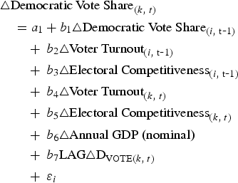
My dependent variable measures change in the normal Democratic vote share in state k at time t. The theoretically-central independent variable measures change in the normal Democratic vote share in state i at time t-1.Footnote 44 The causal relationship between political contagion and a current set of congressional voters can thus be expressed in the following manner:

For each of these variables, change is calculated by subtracting a state's current Democratic vote share from its six-year (three-Congress) prior moving average. For the principal independent variable, deviation from a state's average Democratic vote share (i.e., its departure from the mean) is used as a proxy for the level of unexpectedness generated by the party's prior electoral performance. The larger the difference, the more dramatic and unanticipated the outcome is assumed to be. For the dependent variable, departure from the mean is a measure of the contagion effect produced by that prior performance. All other things being equal, the greater the deviation produced in the prior election, the larger I expect the size of the contagion effect to be.
Several additional explanatory variables are also included to control for competing sources of vote change. Variations in both voter turnout and electoral competitiveness can directly impact the relative vote shares of party contestants. For this reason, I have included measures of change in turnout levels and change in electoral competitive margins for both the current state contest (state k) and for the prior state in the electoral sequence (state i). The turnout variable is a proxy for party mobilization efforts, while competitiveness is used as a measure of the interest and excitement generated by a given contest.Footnote 45 Change is once again estimated as the difference between the current value of each variable and its six-year prior moving average. One additional variable, change in the yearly level of nominal gross domestic product (GDP), was included to capture the influence of changing economic conditions on the partisan vote.Footnote 46 The full regression model is given below.
Equation 1.
Further Issues in Modeling the Interstate Transmission of Political Contagion
Finally, it seems reasonable that three additional factors helped to condition the dissemination of interstate contagion in nineteenth-century congressional elections. First, the level of contagion in a given race was likely affected by the temporal proximity of any two sequential election dates. All other things being equal, the longer the period of elapsed time between two congressional contests, the weaker the transmission of contagion should have been; an electoral outcome occurring months before the next election should exert far less influence than one occurring only days or weeks earlier. Second, the level of contagion was likely conditioned by the spatial proximity of two sequential elections. Especially in the early years of my data set, prior to the advent of the telegraph, information moved more slowly across states. The closer two states were to each other geographically, the more rapidly contagion could spread, which was essential if their election dates also happened to be closely fixed in time. In addition, shared state boundaries are often a proxy for shared interests, attachments, and identities. Thus, all things being equal, the contagion effect of an unexpected party performance in New Jersey's congressional races should exert a greater influence in neighboring New York than in more distant states like Minnesota, Louisiana, or California. Finally, sectionalism was an indelible feature of nineteenth-century American politics. It seems plausible therefore that political contagion arising from a dramatic showing in Virginia's congressional elections would be felt with much greater force in Tennessee or Texas than in Pennsylvania or Iowa. The same proposition should hold true for elections in Northern states.
Regression Results
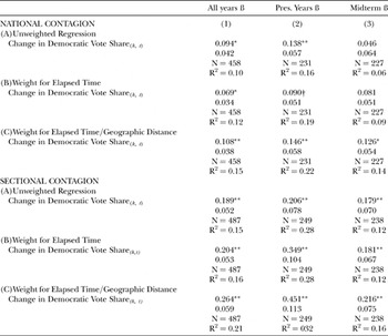
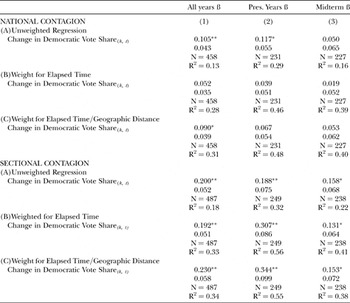
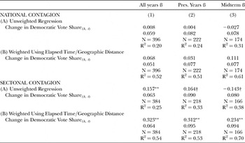
Tables 1, 2, and 3 report the results of my regression analysis. Respectively, the results in each table represent an increasingly stringent test of the political contagion hypothesis. Table 1 presents results based on Equation 1. Table 2 adds an additional set of controls for fixed panel effects by state, while Table 3 controls for both fixed panel effects and fixed time effects by congressional year. Passing the hurdles imposed by each additional test should increase confidence in the robustness of the results reported.
Contagion in Sequential Congressional Elections, 1828–1874

a) OLS regression with panel-corrected standard errors (Stata 7 SE). ** = p < .01; * = p < .05; † = p < .1.
b) Dependent variable is the change in Democratic congressional vote share, estimated as difference between current vote and 3-Congress moving average.
c) Additional explanatory variables were included in the regression analysis, but are not reported above. See page 191 for full specification.
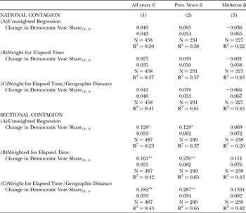
Contagion in Sequential Congressional Elections,1828–1874 (with Fixed Effects by State)

a) OLS regression with panel-corrected standard errors (Stata 7 SE). ** = p < .01; * = p < .05; † = p < .1.
b) Dependent variable is the change in Democratic congressional vote share, estimated as difference between current vote and 3-Congress moving average.
c) Additional explanatory variables and fixed effects indicators were included in the regression analysis, but are not reported above. See page 191 for full specification.
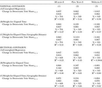
Each table presents estimates for both national and sectional contagion effects.Footnote 47 These estimates are arranged in a single nine-cell matrix: Columns 1, 2, and 3 report coefficients for (1) all years in the data set, (2) presidential years only, and (3) midterm years only; Rows A, B, and C report coefficients for (A) unweighted regression estimates, (B) estimates weighted for the time elapsed in days between two sequential election dates, and (C) estimates weighted for both elapsed time and the geographic distance between two sequential election dates (operationalized as the number of states at time t-1 sharing contiguous borders with a given state at time t). I restrict the tabular presentation of findings to those coefficients that measure the causal influence of interstate contagion on the congressional vote. I have no theoretical expectations regarding other explanatory variables and the vote, so this format will help focus attention squarely on those issues directly under consideration.
Contagion in Sequential Congressional Elections,1828–1874 (with Fixed Effects by State and CG Year)

a) OLS regression with panel-corrected standard errors (Stata 7 SE). ** = p < .01; * = p < .05; † = p < .1.
b) Dependent variable is the change in Democratic congressional vote share, estimated as difference between current vote and 3-Congress moving average.
c) Additional explanatory variables and fixed effects indicators were included in the regression analysis, but are not reported above. See page 191 for full specification.
The findings arrayed in Column 1 of Table 1 indicate the presence of both national and sectional contagion effects on current vote shares. These findings are robust across rows; that is to say, the results do not depend on the presence or absence of the weights. The results further reveal sectional contagion effects at twice the magnitude of national effects. That section trumps nation in this instance makes intuitive sense, given that the period in question is almost coextensive with the years in which slavery, Civil War, and Reconstruction dominated American politics. In the unweighted sectional model, a 10-percentage-point change in the Democratic vote share in state i at time t-1 yields a contagion effect of 1.9 points in current congressional races—a swing in the two-party vote of almost 4 points. The use of weights to account for the effects of elapsed time and geographic proximity increases the substantive power of the contagion effect in theoretically predicted ways. With these factors accounted for, a 10-percentage-point change in the Democratic vote share in state i at time t-1 yields a contagion effect of 2.6 points in current congressional races—a swing in the two-party vote of more than 5 points.
Table 1 also indicates that political contagion exerts a substantially more powerful effect on the congressional vote in presidential election years than in midterm years. I will take up this finding a little bit later in the analysis. For now, several things are worthy of note. First, each of the coefficients in Columns 2 and 3 of the sectional model are statistically significant, providing a robust set of findings for sectional contagion's presence in both presidential and midterm years. Second, presidential contagion effects in Table 1 are always larger than midterm effects, with the magnitude of that difference increasing with the application of weights for elapsed time and geographical proximity. Here a 10-point change in the Democratic vote share yields a sectional contagion effect of 4.5 points in presidential years and 2.2 points in the off-years—a swing in the two-party vote of 9 and 4.4 points respectively.
Additional Tests of Robustness
The results in Table 1 provide initial evidence for a significant contagion effect in nineteenth-century congressional elections. As an additional test of the robustness of these findings, Table 2 reproduces this analysis but includes a set of controls for fixed effects by state. Substantively, this accounts for the criticism that these initial results are unduly influenced by the distinctive institutions, politics, and culture of each state.
The estimates contained in Table 2 differ in significant ways from those in Table 1. Most importantly, they show the sectional contagion model to be substantially more robust than the national model, though the unweighted coefficients for “all years” and “presidential years” in the latter model remain statistically significant and resilient in their substantive values. In addition, the sectional model continues to produce comparatively larger substantive effects, whether the comparison in question is between the no-fixed-effects model in Table 1 or the national fixed-effects model in Table 2. Looking first at the unweighted regression, a 10-point change in Democratic fortunes at time t-1 yields a 2-point sectional contagion effect for all years in the data set, 1.9 points in presidential years, and 1.6 points in off-years. Once again, the addition of temporal and geographical weights significantly improves the performance of the sectional model, with a 10-point change in the prior Democratic vote share producing a 2.3 point sectional contagion effect for all years in the data set, 3.4 points in presidential years—a swing of just under 7 percentage points—and 1.5 points in off-years.
All in all, this second test strengthens our confidence in the sectional contagion model. Table 3 presents one last check on the robustness of our findings. This table again reports results based on the initial regression model, but with controls this time for both fixed panel effects and fixed time effects by congressional year. Each two-year congressional election cycle is its own unique political mix, owing to the waning and waxing of domestic political issues, the ups and downs of the economy, and the oscillating intrusions of international affairs. Table 3 controls for these effects.
The first thing to note in Table 3 is the lack of evidence that remains for a national contagion effect. While most of the coefficients retain their expected direction, they are uniformly small and statistically insignificant. The addition of temporal and spatial weights does nothing to improve the performance of the contagion variable in the national model. The sectional effect, by comparison, continues to perform well. Taking account of elapsed time and geographical proximity, a 10-point change in the Democratic vote share yields a contagion effect of 1.8 points for all years in the data set, 2.9 points in presidential years—a swing of almost 6 percentage points—and 1.3 points in off-years, underscoring once again the seeming importance of the presidential context to the contagion effect.
As an additional check on these findings, I reran the analysis presented in Table 3, substituting congressional election returns drawn from a similar forty-four year time period but generated long after the nationwide implementation of 1T/1M (1944–1998). I then imposed the same sequential election schedule used in the original analysis on the new data (1828–1872). To make the analysis comparable, I confined my analysis to the same set of states found in the original data. Put simply, the idea was that, if a similar “contagion effect” could be generated using congressional returns from states subject to a uniform election schedule, then there would be grounds for doubting the validity of my principal findings.Footnote 48
As Table 4 shows clearly, the results of this test were uniformly negative. In each case, contagion coefficients were substantially smaller and often in the wrong direction. Moreover, in no instance did these coefficients achieve accepted conventional confidence levels of p < .05. These findings were consistent across the variety of controls utilized for national/sectional effects, presidential year/off-year effects, or weighted/unweighted effects. In sum, the sequential election data for 1828 through 1872 yielded substantively significant and statistically valid contagion effects that could not be replicated using data drawn from a period of scheduling uniformity long after the imposition of 1T/1M.
Contagion in Congressional Elections, 1944–1998 (with Full Fixed Effects)

a) OLS regression with panel-corrected standard errors (Stata 7 SE). † = p <.1.
b) Dependent variable is the change in Democratic congressional vote share, estimated as difference between current vote and 3-Congress moving average.
c) Additional explanatory variables and fixed effects indicators were included in the regression analysis, but are not reported above. See page 191 for full specification.
A Digression on the Influence of Presidential Elections on Congressional Contagion: Ballot-Induced or Nationalized Context?
The very pronounced contagion effect discernable in presidential years requires closer consideration. Given the relative magnitude of the effect, it is worth considering why contagion is more pronounced in these election periods than in midterm periods. There are two possible explanations: (1) the climate surrounding presidential elections increased the salience of Congress as a national policymaking institution, thereby deemphasizing the local character of individual district contests and enhancing the interstate context in which contagion thrived; or (2) “contagion” was little more than an institutional artifact of the election process itself—a function of both the prevalence of the party-strip ballot and the tendency of voters to choose their ballots on the basis of partisan preferences in the marquee (i.e., presidential) contest. In an era before official state-printed ballots, each party had the responsibility for printing their own election ballots and distributing them to supporters at the polls.Footnote 49 Each ballot listed only that party's nominees for the offices being contested. It was therefore institutionally difficult (though not impossible) to split one's ticket. By this explanation then, the perception of contagion arose not from the unexpected results of a prior congressional campaign; rather, it was an institutionally-forced presidential coattail effect—a residual effect of the ballot choice for president in the current election period.
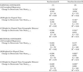
One approach to answering this question requires one to separate out synchronized from non-synchronized elections in this period. If even some portion of “congressional contagion” in presidential years is actually a ballot-induced residuum of the choice for president, it should be discernable by comparing levels of contagion found in each set of states. Voters in states that held both congressional and presidential elections on 1T/1M would have had only one ballot through which to express their partisan preferences for these two federal offices. If the top of the ticket drove the choice of party strips in presidential years—and if that partisan choice differed enough from a voter's normal congressional predilections—the effect might present itself as an “unexpected” change in partisan vote shares for the congressional office. However, if congressional contagion is found to be stronger in the non-synchronized states, then the contagion effect can be more plausibly linked to the heightened national awareness induced by the presidential election context.
Table 5 presents the results of this inquiry. It arranges findings in a manner similar to Tables 1, 2, 3, and 4, save that columns here represent states with synchronous and non-synchronous federal election schedules. In the interest of space, only the results of the full fixed-effects model are reported. Table 5 clearly demonstrates that there is no evidence for “ballot-induced contagion” in presidential years. In both national and sectional models, contagion coefficients in these states are almost never statistically significant; and they are never in the expected direction. All the evidence for the operation of congressional contagion in presidential election years is confined to the non-synchronized states. In the national model, the contagion coefficient is always significant. Unexpectedly, the sectional effect just misses statistical significance at p < .1 in the unweighted model (p = .12), though both weighted sectional models continue to perform well, indeed outperforming the national model effect substantively.
Contagion in Sequential Congressional Elections, 1828–1872: Presidential Years Only (with Full Fixed Effects)

a) OLS regression with panel-corrected standard errors (Stata 7 SE). ** = p < .01;* = p < .05; † = p < .1.
b) Dependent variable is the change in Democratic congressional vote share, estimated as difference between current vote and 3-Congress moving average.
c) Additional explanatory variables and fixed effects indicators were included in the regression analysis, but are not reported in the table above. See page 191 for full specification.
Why is there no evidence for a contagion effect in states with synchronized federal elections? While any answer here must be tentative, I suspect that presidential coattail effects, which are strengthened under conditions of uniform scheduling, might have acted as a countervailing effect on the vote and dampening the measurable effects of contagion. Additional research into this question is needed.
Was Interstate Contagion Confined to Congressional Elections?
Finally, how generalized was this contagion effect in nineteenth-century American elections? Was interstate political contagion peculiar to congressional elections or did it intrude into other electoral realms? I conclude this analysis by briefly taking up these questions.
There are solid reasons to suspect that congressional contagion constituted only one manifestation of a broader period pattern. This expectation is founded on the fact that the sequential character of the congressional election season was not peculiar to the congressional venue. Indeed, in this age of federalism and states' rights, non-synchronous interstate election schedules predominated among the major offices (i.e., the presidential, congressional, and gubernatorial offices) most likely to obtain regional and national attention.
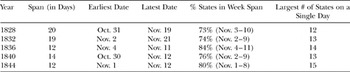
Initially, I turned to presidential elections as the most likely source of the contagion effect. However, the organization of presidential elections militated against the development of interstate contagion, even before they were synchronized nationally in 1848. If we exclude the pre-Jacksonian, pre-partisan era as sui generis, there are only five presidential election periods in which to test.Footnote 50 Additionally, the temporal organization of these five election periods was radically more compressed than congressional seasons, with contests most often occurring within a span of two to three weeks, typically in November. As Table 6 makes clear, between 1828 through 1844, the average number of days between the first and last state presidential contest date averaged only fifteen days. Moreover, this already short time span actually exaggerates the degree of temporal separation in presidential elections. Indeed, within this time frame, the percentage of states holding their presidential elections within the space of a single week averaged a full 77 percent, with the bulk of these scheduled for the same day. Replication of the congressional analysis for presidential elections (not presented here) yields results consistent with the claim that scheduling compression worked actively against the development of a contagion effect in this venue—much as frontloading has been shown to retard the development of momentum in modern presidential primaries—a dampening effect likely compounded by the still rudimentary transportation and communications technologies of the early nineteenth century.
Compression in Presidential Election Scheduling, 1828–1844

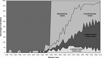
Gubernatorial elections turn out to be a more promising environment in which to test for contagion effects. Like congressional elections, gubernatorial contests remained largely non-synchronized across states through much of the nineteenth century; indeed, they remained so for a substantially longer period of time than their congressional counterparts did. Figure 4 tracks the percentage of states by year that held gubernatorial elections on the first Tuesday after the first Monday in November (of even years). The figure compares that rate with those found for both presidential and congressional elections. It shows that even by as late as 1914, only about 60 percent of the states (twenty-eight of forty-eight by my estimation) had coalesced around that date, as opposed to more than 90 percent of all congressional elections and 100 percent of all state presidential contests.
Percentage of States Holding Elections on the First Tuesday After the First Monday in November (by elective Office).

As gubernatorial elections are even more decidedly local affairs than congressional elections, evidence for an interstate contagion effect here would constitute important supplementary evidence of the political significance of sequential structure on nineteenth century American politics. Indeed, findings by the historian Peter H. Argersinger regarding state legislative contests are suggestive of the importance Populist Party elites placed on the results of early-voting states for their influence in later-voting states.
The People's Party National Executive Committee decided in June to campaign extensively in Kentucky and Ohio where full state tickets were to be elected. . . . Kentucky in particular was vital to Populist hopes, for its election occurred in August, and a good showing there would presumably influence the later elections in Ohio, Iowa, and Nebraska. But if a good showing would encourage the People's party, many feared that the reverse would also be true. … [One] Populist campaigner admitted that the effort to poll a large vote in Kentucky was being made “in order to show members of the party in the Northwest that the Third party movement was taking hold in the South, as well as in that locality.” He declared, moreover, that “the future growth of the party depended largely upon the results in Kentucky,” because a failure there would give the movement “a black eye, and it would demoralize the party's strength in the West.”
Led by John G. Otis and M. W. Wilkins, Kansas Populists actively organized the People's party in Kentucky.Footnote 51
While this is not the place for a full examination of these issues, a brief replication of our prior analysis in this gubernatorial context is at least suggestive of contagion's broader applicability to the era's sequentially-structured electoral politics. The explanatory model used to generate these findings is identical to that used earlier (Equation 1. Data on gubernatorial election dates between 1828 and 1860 were obtained from Michael Dubin's United States Gubernatorial Returns, 1776–1860.Footnote 52 For the years 1861 through 1874, I relied upon annual state election calendars regularly published in the Tribune Almanac and Political Register. Data on gubernatorial returns were likewise found in Dubin and ICPSR no. 7757 (Candidate and Constituency Statistics in the United States, 1788–1990). The dependent variable remains the same (change in the normal Democratic vote share of state k at time t); the key independent variable likewise remains unaltered (change in the normal Democratic vote share state i at time t-1). Additional explanatory variables once again include a lagged dependent variable, change in turnout and competitiveness (both for the current and the last election period), and change in nominal GDP. The time period was held constant (1828–1874) to facilitate comparisons with the results of the congressional contagion analysis. Separate tests were once again run on models with no fixed effects, fixed effects by state, and fixed effects by state and time period.
Table 7 reports only the results of the more stringent full fixed-effects model. Overall, the patterns show a striking consistency with those reported in Tables 1, 2, and 3. Once again, the national contagion model shows no detectable causal relation between prior and current party performance. The unweighted contagion coefficients are uniformly insignificant, both substantively and statistically. By contrast, there is clear evidence of a sectional contagion effect along lines observed earlier. Once again, much of this appears to be the result of the presidential election climate, which though statistically weaker than the coefficient for “all years” in the unweighted model, is still significant at p < .1. More unexpectedly, in light of previous findings, contagion's substantive impact appears to be slightly larger here than in the congressional data set. Here, a 10-point change in prior Democratic gubernatorial fortunes results in a 1.6-point contagion effect in current gubernatorial races. Evidence is lacking for a gubernatorial contagion effect in those time periods coinciding with the congressional midterm cycle, at least when attention is limited to the estimates of the unweighted regression test. Indeed, in this instance, while the midterm coefficient is statistically significant at p < .1, it is not in the expected direction. However, when weights are again applied to account for the combined effects of temporal and spatial distance between election periods, the midterm contagion effect again assumes its theoretically-expected relationship to changes in the Democratic vote share, attaining statistical significance at p < .01.
Contagion in Sequential Gubernatorial Elections, 1828–1874 (Full Fixed Effects Model)

a) OLS regression with panel-corrected standard errors (Stata 7 SE). ** = p < .01; * = p < .05; † = p < .1.
b) Dependent variable is the change in Democratic congressional vote share, estimated as difference between current vote and 3-Congress moving average.
c) Dummy variables for state and time-period effects were included in the regression, but are not reported in the table above.
V. Conclusion
The study of America's non-synchronous nineteenth-century scheduling regime offers more than a history lesson for political scientists. It suggests the broad contours of a fresh research agenda for students of American politics, with implications for those immersed in diverse fields like elections and voting behavior, political party operations, legislative and presidential behavior, and American political development.
First, to summarize my main findings: I have found only modest evidence for the presence of a political contagion effect in nineteenth-century congressional elections when its interstate transmission is modeled as a national phenomenon. However, evidence is substantially stronger for a sectional contagion effect in both presidential and midterm congressional cycles, though the evidence for the latter effect is not as robust as the former. In addition, the application of weights to account for both the time elapsed between election dates and the geographic distance between state contests consistently improves the substantive and statistical power of the sectional contagion model, and it does so in theoretically expected ways. This indicates strongly that the temporal and spatial structure of the sequential cycle itself had important supplemental effects on the level of contagion experienced in nineteenth-century congressional elections. The absence of a contagion effect in the highly compressed environment of presidential elections was shown to be consistent with this claim. Finally, I presented evidence indicating that this nineteenth-century contagion effect was not confined to congressional elections, but also found its way into other sequentially-structured electoral realms, such as gubernatorial elections.
What about future research? A focus on election scheduling regimes could provide leverage on a range of theoretically interesting questions. For example, for students of political parties and mass electoral behavior, such a focus might provide additional insight into the relationship between electoral rules and voter turnout. As Richard Boyd and others have noted, multiple mobilization efforts by political parties divert resources and reduce participation among peripheral voters—ironically, those most dependent on partisan mobilization drives to make it to the polls.Footnote 53 Applied to the nineteenth-century context of this article, several questions are raised. Did state parties that mobilized supporters only once to vote in federal elections bring a substantially higher percentage to the polls than those saddled with multiple mobilization efforts? Or additionally, among the non-synchronous states, did variations in the temporal proximity of congressional and presidential elections further affect voter turnout levels? That is, was turnout progressively depressed as a congressional election was set one month, three months, six months, or more out from that season's presidential contest? Was state congressional turnout affected by whether it was set before or after the presidential election? Finally, did on-year congressional turnout in the non-synchronous states mirror off-year levels, or was there a presidential-year turnout bump regardless of whether the presidential contest was actually on the ballot?
On a different track, the multiplication of ballots caused by non-synchronous elections likely aggravated partisan electoral efforts in still another ways. It provided nineteenth-century American voters with an easy means to split their tickets in federal contests. It is sometimes argued that split-ticket voting in federal elections became structurally possible to a significant degree only with the advent of the secret ballot.Footnote 54 Prior to this, the party-strip ballot format rigidly induced straight party voting. However, once we recognize that nineteenth-century congressional and presidential elections were regularly separated in time—thus institutionalizing the use of separate ballots in the making of one's choices for president and House—it becomes clear that the opportunity to split one's ticket was much more prevalent in nineteenth century America than is currently accounted for in the literature. One easily-tested question is whether in fact voters in the non-synchronous states actually availed themselves of this opportunity, or whether the bonds of party—or, alternatively formulated, whether disciplined party mobilization drives and organized surveillance at the polls—militated against the possibility of splitting one's ticket to any significant degree.
In the area of congressional studies, important new work cognizant of nineteenth-century scheduling practices has already yielded insights. Erik Engstrom and Samuel Kernell argue persuasively that the timing of presidential and House races within states, along with other state electoral laws had a systematic impact on the size of presidential coattails and thus on the number of legislative seats won or lost by the president's party.Footnote 55 State electoral calendars thus had a significant impact on the partisan control of Congress. Still, additional questions remain. For example, did legislative party majorities target early states in the electoral season with legislation, spending, government contracts, patronage, and the like, all in an effort to generate a contagion effect advantageous to that party? Or, following Jonathan Katz and Brian Sala's lead, did congressional careerism gain an early foothold in states where separation in time from the presidential vote allowed incumbent legislators the leeway to cultivate a personal vote?Footnote 56 Still further questions suggest themselves: How did non-synchronous scheduling affect internal legislative dynamics? Did sequential scheduling in congressional elections affect the scheduling of bills in Congress? Were legislative votes timed to influence early elections and generate interstate contagion? How did the elongated temporal rhythm of the congressional election season affect legislative party discipline?Footnote 57
Finally, each of these issues is linked to deeper historical questions about the sources and developmental consequences wrought by American scheduling regime change. How did the new national uniformity in federal election calendars and the disappearance of sequential elections alter the mobilization strategies of organized groups and social movements seeking access to political elites? Who gained power and who lost it under the new rules, and with what political ramifications? What impact did an increasingly synchronized electoral calendar have on the evolving organizational characteristics of American political parties, the country's representative institutions, and the nineteenth-century patronage state? Each was deeply enmeshed in the incentives and rhythms of nineteenth-century electoral politics; perhaps not coincidentally, each began to experience changes to its basic organizational structure in tandem with the national adoption of the 1T/1M rule.Footnote 58
In all, a host of fresh perspectives on American electoral behavior, party operations, and institutional development are opened up to view once scholars become cognizant of the specific historical character of this unique nineteenth-century U.S. scheduling regime.