INTRODUCTION
In agricultural ecosystems, the organic matter cycle is impaired due to continuous crop harvesting and enhanced decomposition processes, related to conventional agricultural practices. The decrease in soil organic matter reduces soil fertility and enhances erosion and desertification, particularly in the Mediterranean area (Geeson et al. Reference Geeson, Brandt and Thornes2002; Fernández et al. Reference Fernández, Plaza, García-Gil and Polo2009; González-Ubierna et al. Reference González-Ubierna, Jorge-Mardomingo, Carrero-González, de la Cruz and Casermeiro2012). In recent years, compost amendment of agricultural soils has been adopted in order to improve soil physico-chemical and biological properties, recovering soil fertility of degraded agricultural ecosystems (Garcia-Gil et al. Reference Garcia-Gil, Plaza, Soler-Rovira and Polo2000; Albiach et al. Reference Albiach, Canet, Pomares and Ingelmo2001; Whalen et al. Reference Whalen, Hu and Liu2003; Bastida et al. Reference Bastida, Kandeler, Hernández and Garcia2007; Iovieno et al. Reference Iovieno, Morra, Leone, Pagano and Alfani2009). Moreover, compost production is particularly attractive as a way to reduce the organic waste landfill disposal or incineration and the consequent environmental impacts. Compost application has been shown to increase the soil organic matter content and nutrient availabilities, to enhance soil microbial activity and to improve a variety of soil physical and chemical properties. However, in order to obtain positive agronomic effects and ensure an environmentally safe use of compost, its chemical quality (Doelsch et al. Reference Doelsch, Masion, Cazevieille and Condom2009), the quantities and dynamics of nutrients (Baldantoni et al. Reference Baldantoni, Leone, Iovieno, Morra, Zaccardelli and Alfani2010b ) and potential pollutants (Baldantoni et al. Reference Baldantoni, De Nicola and Alfani2010a ) should be monitored. The presence of pollutants in compost, depending on starting material characteristics and processing methods, represents a potential threat because pollutants can alter soil ecosystems and enter food webs. The fate of heavy metals in soils treated with compost has been widely investigated (Smith Reference Smith2009), but long-term dynamics of organic contaminants also need to be considered (Petersen et al. Reference Petersen, Henriksen, Mortensen, Krogh, Brandt, Sorensen, Madsen, Petersen and Grøn2003; Cai et al. Reference Cai, Mo, Wu and Zeng2008; Baldantoni et al. Reference Baldantoni, De Nicola and Alfani2010a ). Indeed, compost application could not only be a source of organic pollutants in agricultural soils, but could also promote degradation of some types (Kästner & Mahro Reference Kästner and Mahro1996; Puglisi et al. Reference Puglisi, Cappa, Fragoulis, Trevisan and Del Re2007), such as polycyclic aromatic hydrocarbons (PAHs), by improving the soil environment for the microbial community and enhancing its decomposing activity (Semple et al. Reference Semple, Reid and Fermor2001). Despite the amount of available data, a whole model for the relationships among compost application and the dynamics of the soil properties has never been developed. Most of the knowledge on these topics, indeed, derives from the analysis of simple bivariate relationships that do not consider the effects of multiple interacting variables. Although it is possible to build useful models for the dynamics of the soil properties following compost amendment using conventional multivariate techniques, this approach is not tailored to test and describe structural relationships of cause and effect (Shipley Reference Shipley2004). As a consequence, the derived models could lack ecological significance while still being useful as descriptive and predictive tools. In order to derive models that are faithful representations of the ecological interactions among the studied parameters, it is thus necessary to include the notion of causality into the analyses, through different analytical methods relying on graph theory.
Path analysis can be used both for confirmatory model testing and for exploratory model building, and Shipley (Reference Shipley2000a ) has given an in-depth description of the main techniques of path analysis including the use of structural equation models and d-sep tests for confirmatory analysis. Both these strategies have advantages and drawbacks: while the exploratory methods derive the most probable causal structure easily and powerfully from the data, the confirmatory approach allows testing of different hypotheses and thus inferences to be drawn about the underlying processes of the causal structure. Among the techniques used to test causal hypotheses, the structural equation model (Shipley Reference Shipley2000a ) has many advantages over the d-sep tests (Shipley Reference Shipley2000a , Reference Shipley b , Reference Shipley2003, Reference Shipley2004), such as the possibility of including unmeasured variables and undirected co-variances in the models, as well as the availability of many reliable software to perform the analyses. However, the structural equation model is a maximum-likelihood technique that gives asymptotic estimates; therefore, it suffers the heavy drawbacks of requiring a very large minimum sample size and in assuming multivariate normality of the data as well as linearity of the functional link between the variable pairs. The d-sep tests overcome these limitations by relying on the graph theoretic notion of d-separation (Pearl & Verma Reference Pearl, Verma, Forbus and Shrobe1987; Geiger et al. Reference Geiger, Verma and Pearl1990; Geiger & Pearl Reference Geiger and Pearl1993; Pearl Reference Pearl2000) that holds independently of the distributional properties of each variable and the functional form of the equations linking the variables in the models (Shipley Reference Shipley2004). Moreover, the d-sep tests, relying on tests of conditional independence, usually require small minimum sample size and allow the choice of different tests to account for the distributional properties of the variables and the functional links among them.
Since many hypotheses on the structural relationships among the soil property dynamics following compost amendment are available from the literature, it is possible to theoretically derive a set of causal hypotheses to be tested. With the aim of developing a causal model for the dynamics of soil organic matter, nutrients, PAHs and microbial activities in relation to compost applications, the present paper followed this approach by testing (with the d-sep tests) a set of hypotheses using the dataset of a 3-year experiment on compost amendment of an agricultural soil in Southern Italy (Iovieno et al. Reference Iovieno, Morra, Leone, Pagano and Alfani2009; Baldantoni et al. Reference Baldantoni, De Nicola and Alfani2010a , Reference Baldantoni, Leone, Iovieno, Morra, Zaccardelli and Alfani b ).
MATERIALS AND METHODS
Experimental stations and laboratory analyses
The field trials were carried out in a typical intensive agricultural system in Southern Italy (40°34′N, 14°58′E, 65 m asl), whose soil is classified as a Clay Gleyc Luvisol (FAO 1998). The field was divided, according to a randomized block design, in plots (10×7 m each) amended with 0, 15, 30 and 45 t/ha (dry matter) of compost, with three replications for each compost dose. The certified quality compost, according to Italian law, was incorporated annually in spring, from 2002 to 2005, into the first 20–25 cm of soil with a rototiller (Lombardini LDA97, Reggio Emilia, Italy).
Annually, 8–9 months after compost application, soil samples (0–20 cm depth) were collected from each plot, sieved (2 mm) and stored at 4 °C until biological analyses, oven-dried at 75 °C for organic matter and element analyses, or air-dried for PAH analyses.
Organic matter content was estimated using loss on ignition (4 h, 550 °C) with a Nabertherm Controller B170 oven. A brief description of the methods applied to measure the other variables used in the models is reported below; further details are given in Baldantoni et al. (Reference Baldantoni, De Nicola and Alfani2010a , Reference Baldantoni, Leone, Iovieno, Morra, Zaccardelli and Alfani b ) for element and PAH concentrations and in Iovieno et al. (Reference Iovieno, Morra, Leone, Pagano and Alfani2009) for microbial activities.
Owing to the large number of chemical elements measured, a preliminary screening was required in order to reduce the complexity of the causal models. Only the elements that showed the largest variation over the 3 years of the study (as total or available concentrations) among the compost doses were selected for inclusion in the models. Based on such criteria, potassium (K) and zinc (Zn) available concentrations, analysed using flame atomic absorption spectrometry on soil extracts obtained according to the Goldberg & Farini (Reference Goldberg and Farini1994) and the Lindsay & Norvell (Reference Lindsay and Norvell1978) methods, respectively, were selected.
Respiration, considered as a proxy of microbial activity, was chosen for inclusion in the models rather than specific enzymatic activities. Otherwise, several respirometric tests have been used to investigate the effects of compost on degradation of organic contaminants (Hupe et al. Reference Hupe, Lüth, Heerenklage and Stegmann1996; Sayara et al. Reference Sayara, Borrás, Caminal, Sarrá and Sánchez2011). Soil microbial respiration was measured using GC as CO2 concentration in the head space of sealed vials, after incubation of soil samples (48 h, 25 °C) in darkness.
In order to keep the models as simple as possible, the PAH concentrations were reported as total PAHs. Total PAH (sum of naphthalene, acenaphthylene, acenaphthene, fluorene, phenanthrene, anthracene, fluoranthene, pyrene, benzo[a]anthracene, chrysene, benzo[b+k]fluoranthene, benzo[e]pyrene, benzo[a]pyrene, perylene, indeno[1,2,3-c,d]pyrene, dibenzo[a,h]anthracene and benzo[g,h,i]perylene) concentrations were detected using GC–MS on soil samples extracted by sonication in a mix of dichloromethane:acetone (1 : 1=v:v).
d-sep tests
According to Shipley (Reference Shipley2009), the steps in performing the confirmatory path analysis through the d-sep tests are the following:
-
– Express the hypothesized causal relationships between the variables in the form of a directed acyclic graph (DAG).
-
– List each of the k pairs of variables in the graph that do not have an arrow between them.
-
– For each of the k pairs of variables (X i , Xj ), list the set of other variables, {Z} in the graph that are direct causes of either X i or X j . The pair of variables (X i , Xj ) along with its conditioning set {Z} define an independence claim (X i , Xj )|{Z}, and the full set of the k independence claims defines the basis set B U.
-
– For each element in this basis set, obtain the probability, p k , that the pair (X i , Xj ) is statistically independent conditional on the variables Z.
-
– Combine the k probabilities using the equation:
 $$C = - 2\sum\limits_{i = 1}^k {{\rm ln(}p_i )} $$
and compare the resulting C value to a χ 2 distribution with 2k degrees of freedom. Reject the causal model if the C value is unlikely to have occurred by chance.
In relation to the complexity of the model, the analyses can require the test of many independence claims, their number in the basis set B U being calculated as follows (Shipley Reference Shipley2009):
 $$N = \displaystyle{{V!} \over {2(V - 2)!}} - A$$
where V is the number of variables (i.e. vertex) and A the number of direct interactions (i.e. arrows) in the causal model. Manually testing such a number of conditional independence claims and aggregating the results, while giving the researcher the full control of the analysis, is a time-consuming and error-prone practice. To avoid the accumulation of accidental errors during the analyses and to allow a high analytical throughput, a computer script (‘cpa’) was then developed (available from the authors and in the ‘cpa’ package at the CRAN website http://cran.r-project.org/). The R programming language (R Development Core Team 2013) was chosen due to the availability of many reliable functions to perform the statistical analyses, its capability to easily handle matrices and the current authors’ familiarity with it. Another package (‘ggm’; Marchetti et al. Reference Marchetti, Drton and Sadeghi2012) for the R programming environment with functions to perform the d-sep tests is available at the CRAN website. However, the cpa and the ggm packages implement the above-mentioned algorithm differently, the most important difference being the way in which the conditional independence claims are tested. Indeed, while the ‘shipley.test’ function of the ggm package performs a Pearson's partial correlation test, the cpa function performs a least square regression, as detailed below. Due to the need to calculate the covariance matrix in the shipley.test function, the presence of missing data imposes the deletion of entire rows in the data matrix, and thus reduces the degrees of freedom for all the conditional independence tests. In contrast, cpa handles missing data by removing only the rows in the matrices of the models that contain them. As a consequence, the sample size and the degrees of freedom are reduced by the presence of missing data only in the models involving variables that contain them, preserving a greater sample size for all the others. This feature indirectly improves the statistical power of the Fisher's C test performed by cpa over that of ggm by preserving a greater power for part of the conditional independence tests. In addition, the calculation of the Akaike Information Criterion (AIC) statistic (according to Shipley Reference Shipley2013) is already implemented in cpa, as well as the structured regressions for each direct path. Indeed, since the demonstration that the Fisher's C statistic is a maximum-likelihood estimate (Shipley Reference Shipley2013), it is possible to calculate the AIC or its version corrected for small sample sizes (AIC c ) for any model, according to the equations:
 $${\rm AIC} = C + 2K,$$
 $${\rm AIC}_c = C + 2K\left( {\displaystyle{n \over {n - K - 1}}} \right),$$
where C is the Fisher's C, K the total number of parameters associated with each path model and n the total number of observations in the data matrix. Owing to the differences mentioned above, a comparison of the Fisher's C statistic obtained using the two software packages was performed.
Software description
The cpa script, with a simple T cl /T k graphical interface, accepts as input files the data matrix, the list of variables (V) in the model and the list of direct interactions (A), expressed as vectors of two variables, ordered as A i =(parent i , child i ). The program searches for all pairs of variables (X i , Xj ) that do not share an arrow between them and lists the pairs in a dataset (B). All direct causes of each variable in each pair are then searched using the A list and stored in vectors {Z i } inside a list. Tests of conditional independence are then performed by regressing X j on X i plus the set of conditioning variables {Z i } using the function ‘lm’ of the stats package and each test is stored in a list (T). The choice of the lm function was driven by the non-hierarchical structure of the data and by the small number of observations per variable in the dataset, insufficient to perform non-parametric (form free) regressions. Other parametric models, such as nonlinear or polynomial regressions, were also avoided due to the difficulties in automatically selecting a parametric function and in deriving the parameters needed to calculate the null probability for each test of conditional independence. Partial P i values of X i are extracted with the ‘summary.lm’ function, stored in a vector of length k, and used to calculate the C value according to Eqn (1). The C value is compared to a χ 2 distribution with 2k degrees of freedom and the model is accepted if P C >α, for α=0·05. The AIC of the model is calculated according to Eqn (4), where the total number of parameters is calculated as the sum of the number of parameters estimated for each structural equation (K i ). Due to the modelling of the structural equations as multiple linear models with an intercept, K i is calculated as the number of independent variables plus 2 (the intercept and the residual error). Finally, each structural equation is fitted with the observational data and the results are stored in a list (T dc ). The C, P C and AIC values are eventually printed out along with an informative message, and the list of conditional independence tests T, the dataset B U, with the calculated P i value for each independence claim and the list of the fitted structural equations T dc , are stored for researcher control of the results.
RESULTS
Data set description
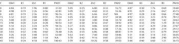
The dataset, reported in Table 1, consisted of 12 observations (three replicates for each compost dose) and 16 variables, with two missing data.
Dataset used for the analyses (three replicates for each compost dose)

C, compost dose (t/ha); OM, organic matter content (g/100 g DW); K, available K concentration (mg/g DW); Zn, available Zn concentration (μg/g DW); R, soil microbial respiration (μg CO2/g DW/h); PAH, polycyclic aromatic hydrocarbon concentrations (ng/g DW). Variables are numbered sequentially according to the year they refer to (first, second or third); NA, not available.
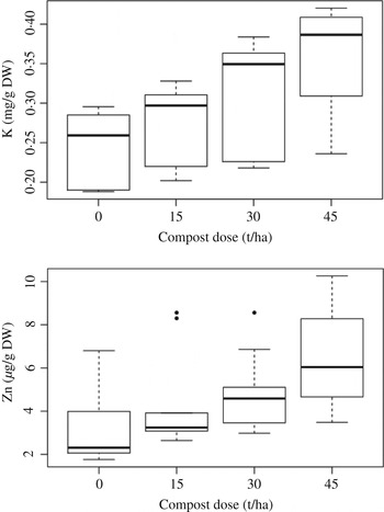
The available concentrations of K and Zn were chosen to be included in the models because of their wide variations along the compost doses (Fig. 1). Soil organic matter content was weakly affected by compost amendments during the years of experimentation (Table 1). Available K and Zn concentrations as well as microbial respiration increased with a dose-related effect, showing the largest increases in the second year for K and in the third for Zn and respiration (Table 1). The PAH concentrations increased after the first compost amendment, particularly in 45 t/ha plots. In the second year, PAH concentrations showed a further increase in the soils amended with 15 and 30 t/ha, whereas a decrease was found in 45 t/ha plots. In the third year, a general decrease in PAH concentrations was found in all the amended plots, especially in 30 and 45 t/ha, with values lower than in 0 t/ha plots (Table 1).
Available K and Zn (in the 3 years of the study) relationships with compost dose. Boxes indicate the interquartile ranges, bold lines the medians and circles the outliers.

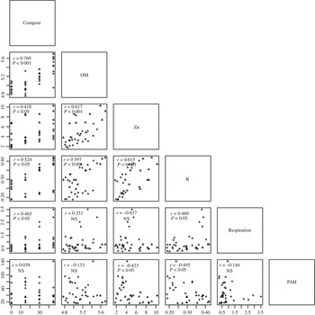
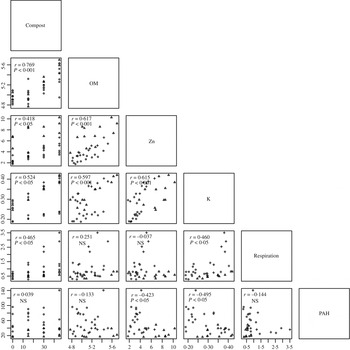
Figure 2 shows the bivariate trends between the six variables considered in the present study that, within each year, were mostly linear.
Scatter plot data semi-matrix of compost doses (t/ha), organic matter (g/100 g DW) content, available K (mg/g DW) and Zn (μg/g DW) concentrations, microbial respiration (μg CO2/g DW/h) and PAH (ng/g DW) concentrations in the 3 years of the study (circles: first year, triangles: second year, cross-hairs: third year). Pearson's correlation coefficient and the associated probability are also reported for each bivariate relationship; NS, not significant.
Model descriptions
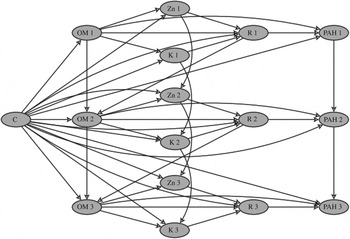
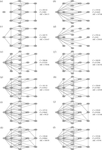
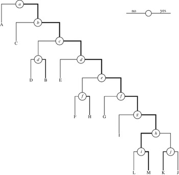
Thirteen hypothetical models were expressed as DAGs and analysed for compatibility with the observational data using the d-sep test approach. Since many of the causal hypotheses developed led to the formulation of feedback loops, and thus to cyclic graphs not suitable for the d-sep test analysis, the time dependency of the models was made explicit by splitting each variable into three other variables, each referring to one of the 3 years of the experiment. Based on the observed patterns and the current knowledge of the processes related to compost amendments, it was possible to develop the model (M) in Fig. 3. In this model, it was hypothesized that compost amendments directly influence all the other variables; the organic matter in turn influences the availability of K and Zn, as well as the respiration and the concentration of PAHs. Soil respiration influences the organic matter content in the following year and the PAH concentrations in the same year. In addition, it was supposed that in the second and third years the organic matter content, the K and Zn available fractions and the PAH concentrations depend on their values in the previous year. In Fig. 4, there are null or alternative hypotheses in respect of some relationships supposed in the DAG represented in Fig. 3. A classification tree for these models, based on ten criteria, is given in Fig. 5, showing the logical relationships among them and the directions in the model space that minimize the AIC. In particular, graphs (a) and (b) of Figs 4 and 5 represent the null hypotheses that the compost amendments do not influence any other variable and that there is no influence among the years, respectively. In graph (c), compost amendments influence the dynamics of the other variables through affecting the organic matter content only, while in graphs (d)–(h) the hypothesis expressed in (d), i.e. compost is a direct cause of all the other variables and no relationships among these are present, is progressively relaxed. Graph (i) lacks the relationship between respiration in each year and organic matter content in the following one, whereas in graphs (j) and (k) two alternative hypotheses about the influence of the microbial respiration on the PAH concentrations through the years are expressed. Finally, model (l) lacks the direct interactions between the organic matter content and the PAHs in each year.
Model (M) describing the most probable (Fisher's C statistic=112·74, P=0·9861, AIC=84·74) explanation of the causal relationships among the six variables considered in this study. C, compost dose (t/ha); OM, organic matter content (g/100 g DW); Zn, available Zn concentration (μg/g DW); K, available K concentration (mg/g DW); R, soil microbial respiration (μg CO2/g DW/h); PAH, polycyclic aromatic hydrocarbon concentrations (ng/g DW). Variables are sequentially numbered according to the year they refer to (first, second or third).

Alternative hypotheses explaining the causal relationships among the six variables considered in the present study. Fisher's C statistic (C), the probability (P) and the AIC for each model are also reported on the right side. C, compost dose (t/ha); OM, organic matter content (g/100 g DW); Zn, available Zn concentration (μg/g DW); K, available K concentration (mg/g DW); R, soil microbial respiration (μg CO2/g DW/h); PAH, polycyclic aromatic hydrocarbon concentrations (ng/g DW). Variables are sequentially numbered according to the year they refer to (first, second or third).

Classification tree for the models in Figs 3 (M) and 4 (A–L). To each node is associated one of the following criteria (indicated by small letters), a positive answer moves to the right and a negative one to the left; thick lines indicate the directions that minimize the AIC. (a) Compost influences other variables; (b) compost directly influences all the other variables; (c) temporal relationships exist; (d) inter-variable relationships exist; (e) OM influences other variables; (f) nutrients influence other variables; (g) respiration influences OM; (h) respiration influences PAHs in the following year; (i) OM influences PAHs; (j) respiration influences PAHs in the same year.

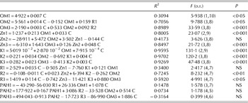
The graph in Fig. 3 had the highest P-value among the developed DAGs, whereas graphs (a) and (c) (Fig. 4) had the lowest. Graphs (d)–(h) showed increasing P-values, according to their complexity, and graphs (i)–(l) (Fig. 4), approximated, in relation to their probability, the results obtained from model M (Fig. 3). The basis set for the model in Fig. 3, together with the null probabilities for each independence claim, is reported in Appendix A. Only four out of the 74 multiple linear models employed to test the relative conditional independence statements had P<0·05, indicating conditional association between the involved variables. The lowest AIC value (84·74) was obtained for the DAG of Fig. 3, whereas the highest ones pertained to the models in Fig. 4 (a–c), showing values about three-fold higher. Since it had the highest probability and the lowest AIC, model M was chosen as the best representation of the ecological processes that follow compost amendment. The structural equations implied by this model were then derived and the fitting results are reported in Table 2. Since the relationships between each pair of variables were mostly linear (Fig. 2), and to avoid overfitting of the data, the structural regressions were modelled as multiple linear models. Despite the agreement of model M with the observational data, five structural regressions were not significant. In particular, the respiration in the first year, the Zn concentration in the second year and the PAH concentrations in each of the 3 years cannot be predicted based on the chosen causal structure.

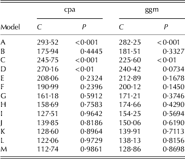
The data provided in Table 3 highlighted that the results obtained with the cpa package were similar to those obtained using the ggm package, although the latter tended to produce more conservative results, above all for the more complex models.

DISCUSSION
There are many alternative causal hypotheses that are able to explain the observed data; however, considering the probability of each model and their AICs, the causal process expressed by model M is probably the best representation of the causal relationships linking the considered variables. Both the software packages employed, moreover, produced the highest probability for this model, ensuring the reliability of this result. As detailed below, the developed model confirms most of the fragmented knowledge on the effects of compost application in agricultural soils and, in addition, represents an integrated model of the interactions among the considered parameters. In evaluating the strength of each causal interaction in the model, some useful information can be revealed by comparison with the other hypotheses. In particular, compost amendment is probably the most important determinant for the dynamics of the other variables, since its exclusion (model A) led to the smallest probability (P=5·03×10−7) and the highest AIC among the 13 DAGs developed. Equally, the influence of compost amendment through the changes in the organic matter alone (model C) is not sufficient to obtain a significant model, indicating that compost application is directly responsible for the dynamics of available K and Zn, of microbial respiration and of PAH concentrations. Numerous studies have demonstrated an increase in the organic matter content and nutrient availabilities in agricultural soils following compost amendments (Weber et al. Reference Weber, Karczewska, Drozd, Licznar, Licznar, Jamroz and Kocowicz2007; Castro et al. Reference Castro, Nas and De las Heras2009; Nayak et al. Reference Nayak, Patel, Ramakrishnan, Mishra and Samantaray2009; Diacono & Montemurro Reference Diacono and Montemurro2010), so compost is widely employed in restoration of agricultural soils (Ros et al. Reference Ros, Hernandez and García2003). The increase in soil nutrient availabilities following compost amendment (Wong et al. Reference Wong, Ma, Fang and Cheung1999), however, is not only an organic matter-mediated effect, through the changes in the exchange complexes (Zheljazkov & Warman Reference Zheljazkov and Warman2004), but also a direct effect of compost nutrient contents (Pinamonti et al. Reference Pinamonti, Stringari, Gasperi and Zorzi1997; Soumaré et al. Reference Soumaré, Tack and Verloo2003). Similarly, soil microbial activity can also be enhanced by compost amendment (Nayak et al. Reference Nayak, Patel, Ramakrishnan, Mishra and Samantaray2009; Diacono & Montemurro Reference Diacono and Montemurro2010) through the addition of both decomposable substrates and exogenous microorganisms (Garcia-Gil et al. Reference Garcia-Gil, Plaza, Soler-Rovira and Polo2000). Moreover, the increase in nutrient availabilities after compost application is also reported to produce beneficial effects on soil microbial activity (Borken et al. Reference Borken, Muhs and Beese2002).
Other pivotal relationships in the model are those among the organic matter content, the available K and Zn concentrations, the microbial respiration and the PAH concentrations, since their complete exclusion (model D) led to rejection of the model. The increase of inter-relationships among the above-mentioned variables in models E–H, in contrast, lowers the AIC of the models, increasing the likelihood of the causal hypotheses they represent. This finding was not unexpected, since the tight relationships among the above-mentioned variables are widely reported in the literature.
The interactions of organic matter content and respiration through the years, as well as nutrient and PAH concentrations, are also important: their complete exclusion (model B), while determining an acceptable model, largely decreases its significance in relation to the most probable model (model M). The inclusion or exclusion of: (i) the direct interactions between the organic matter content and the PAH concentrations (model L), (ii) the interactions between respiration in each year and the organic matter content in the following year (model I) and (iii) the changes in the temporal relationships between the respiration and the PAH concentrations (models J and K), determine slight deviations from the best model, indicating that all these relationships could be of marginal importance in determining the observed patterns.
Other useful information for evaluating the strength of each direct path is revealed by the structural equations reported for the best model. In particular, the model explains a great percentage of the variance in the concentrations of K and Zn (with the exception of the second year) and in the organic matter content, indicating that their dynamics are determined to a great extent by the hypothesized causal process. For the latter parameter, it is worth mentioning the increase in fitting performance from the first to the third year, probably indicating that the processes described by the model increase in strength after subsequent compost additions. However, respiration and, even more, PAH concentrations are poorly predicted by the model, suggesting that other causes of variation can determine their dynamics. A decrease in organic pollutant concentrations following soil compost amendment was often observed (Puglisi et al. Reference Puglisi, Cappa, Fragoulis, Trevisan and Del Re2007; Haritash & Kaushik Reference Haritash and Kaushik2009). It was generally attributed to the enhanced microbial activity as a consequence of carbon and energy sources and nutrient inputs as well as amelioration of soil physical properties (Hupe et al. Reference Hupe, Lüth, Heerenklage and Stegmann1996; Scelza et al. Reference Scelza, Rao and Gianfreda2007; Haritash & Kaushik Reference Haritash and Kaushik2009; Yang et al. Reference Yang, Zhang, Xue, Lu and Tao2011). The sequestration of organic pollutants by soil organic matter (Kästner & Mahro Reference Kästner and Mahro1996; Sweetman et al. Reference Sweetman, Valle, Prevedouros and Jones2005) may also decrease the measurable PAH concentrations (Scelza et al. Reference Scelza, Rao and Gianfreda2007), their bioavailability and thus their toxicity (Weissenfels et al. Reference Weissenfels, Klewer and Langhoff1992; Gandolfi et al. Reference Gandolfi, Sicolo, Franzetti, Fontanarosa, Santagostino and Bestetti2010). For these reasons, compost is widely employed to improve the bioremediation of PAH contaminated soils (Sayara et al. Reference Sayara, Borrás, Caminal, Sarrá and Sánchez2011). An interaction between the organic matter content and the PAH concentrations is considered in the best model, but, as described above, it determines only a slight increase in the probability of the causal structure.
For the proper evaluation of the current findings, the limited sample size available for the analyses should also be considered. This aspect, while challenging for the analyses, reduces the statistical power of the tests and could limit the power to detect some interactions and the modelling of nonlinear relationships. It is possible, indeed, that some of the supposed interactions, such as those involving the respiration and the PAHs, were not properly evaluated due to the few observations available and the constraints on using only linear models. It is even possible, in addition, that some of the models failed to be rejected due to the low statistical power of the employed tests. A similar situation may pertain to the models with the lowest probability, but it is unlikely to affect the overall results appreciably. Indeed, while the confidence on the models with the lowest probability must remain quite modest, the high probability and reduction in AIC of the best model give sufficient confidence to consider it as a good representation of the described ecological interactions. Despite the limitations, the model developed was able to provide a useful descriptive, and partly predictive, tool for the understanding of the complex effects of repeated compost amendments on soil properties.
Massimo Zaccardelli performed the field trials. Daniela Baldantoni, Flavia De Nicola and Paola Iovieno performed the laboratory analyses. Alessandro Bellino and Daniela Baldantoni developed the software and the causal hypotheses, tested the models and wrote the text with the contribution of Anna Alfani, Flavia De Nicola and Paola Iovieno. Anna Alfani coordinated the work.