



1. Introduction
The air–sea interface mediates the global climate system by regulating the transport of mass, momentum and energy between the atmosphere and the ocean. This exchange is driven by a myriad of fluid-dynamic processes spanning multiple scales, including sea spray, boundary-layer turbulence, buoyant plumes and both surface and internal waves (Sullivan & McWilliams Reference Sullivan and McWilliams2010). Among these, wind-induced surface fluctuations, commonly known as wind waves, are ubiquitous and determine the hydrodynamic roughness of the marine environment. Despite nearly a century of extensive theoretical, experimental and numerical investigations, the underlying mechanisms of wind–wave interactions remain incomplete. The intense, two-way coupling between the turbulent airflow and the compliant water surface imposes severe analytical and numerical challenges, leaving the precise dynamics of wave growth and evolution an enduring problem in environmental fluid mechanics.
The historical trajectory of wind-wave generation research is anchored by three foundational theories. Jeffreys (Reference Jeffreys1925) pioneered the separation sheltering hypothesis, which posits that airflow separates over sharp wave crests, creating an asymmetric surface pressure distribution that transfers energy to the waves. Decades later, Phillips (Reference Phillips1957) and Miles (Reference Miles1957) revolutionised the field with two complementary frameworks. Phillips (Reference Phillips1957) demonstrated that the initial, linear stage of wave growth is driven by the resonance of turbulent atmospheric pressure fluctuations with the water surface. Subsequently, the exponential growth stage is governed by the Miles shear-flow instability mechanism (Miles Reference Miles1957), in which energy is transferred via wave-induced normal pressure ascribed to a critical layer where the mean wind speed matches the wave phase speed. Together, these pivotal mechanisms establish the classic paradigm of wind-wave inception and growth, distinguishing between external turbulent pressure resonance and self-excited shear instability.
To quantify and validate these theoretical mechanisms, extensive experimental and numerical investigations have focused on turbulent flows over both stationary and moving wavy boundaries (Zilker et al. Reference Zilker, Cook and Hanratty1977; Zilker & Hanratty Reference Zilker and Hanratty1979; Hudson et al. Reference Hudson, Dykhno and Hanratty1996; Sullivan et al. Reference Sullivan, McWilliams and Moeng2000; Yang & Shen Reference Yang and Shen2010; Druzhinin et al. Reference Druzhinin, Troitskaya and Zilitinkevich2012; Akervik & Vartdal Reference Akervik and Vartdal2019; Zhang et al. Reference Zhang, Wang and Liu2022a
,
Reference Zhang, Wu, Liu and Wangb
). Over a stationary wavy wall, flow separation induces a highly non-uniform pressure distribution that mimics the sheltering mechanism proposed by Jeffreys. For flows over a moving wavy boundary, a comparable aerodynamic coupling occurs where waves extract momentum from the wind through the correlation between wave-coherent pressure and the surface slope – a process macroscopically quantified as form drag (Akervik & Vartdal Reference Akervik and Vartdal2019). Although the momentum exchange at this compliant interface remains intricate, evaluating the energy flux offers a more direct path to assessing wave growth. Theoretical formulations dictate that the net energy transferred to the substrate results from the integrated work done by both normal pressure and tangential viscous stress against the wave orbital velocity, as illustrated in figure 1. For surface gravity waves, the spectral energy density is traditionally expressed as a function of the angular frequency
 $\omega$
and propagation direction
 $\sigma$
(Komen et al. Reference Komen, Cavaleri, Donelan, Hasselmann, Hasselmann and Janssen1994; Grare et al. Reference Grare, Peirson, Branger, Walker, Giovanangeli and Makin2013), given by
 \begin{align} E(\omega ,\sigma )=\frac 12\rho _wg\iint {a^2(\omega ,\sigma )}\,{\rm d}\omega\,{\rm d}\sigma , \end{align}
where
 ${\rho }_{w}$
is the water density,
 $g$
is the acceleration due to gravity and
 $a$
is the wave amplitude. The variation of
 $E$
controls the development of surface waves, which can be described by the wave energy conservation equation:
 \begin{align} \frac {{\rm d}E}{{\rm d}t}={{S}_{\textit{in}}}+{{S}_{nl}}-{{D}_{d}}, \end{align}
where
 $S_{\textit{in}}$
stands for the wind energy input,
 $S_{nl}$
represents the nonlinear wave–wave interactions that redistribute energy across the spectrum and
 $D_d$
signifies the energy dissipation mediated by wave breaking and viscous effects.
Sketch of the work rate exerted by wind stress on the surface wave velocity at (a) the windward side and (b) the leeward side. The decomposition is shown in the wave-following curvilinear coordinate system.

Figure 1. Long description
A diagram of the work rate exerted by wind stress on the surface wave velocity. Panel A: The windward side. The diagram shows a wavy boundary with wind blowing from left to right. The wave is depicted with a curvilinear coordinate system. Key components include the wind stress (τ), the wave-coherent pressure (p), and the surface wave velocity (u_s and w_s). Arrows indicate the direction of these forces and velocities, with red arrows representing the wind stress and blue arrows representing the surface wave velocity. The diagram illustrates how wind stress and pressure interact with the wave at the windward side. Panel B: The leeward side. Similar to Panel A, this diagram shows the interaction of wind stress, pressure, and surface wave velocity but at the leeward side of the wave. The same color coding and arrow directions are used to represent the forces and velocities. The diagram highlights the aerodynamic coupling and the process of momentum exchange between the wind and the wave, which contributes to wave growth and form drag.
As illustrated in figure 1, we consider the wind flow over a propagating wave with a sinusoidal profile
 $\eta$
and phase speed
 $c$
. The energy input term,
 $S_{\textit{in}}$
, representing the rate of work done by the atmospheric surface stress on the compliant water surface, is defined as
 \begin{align} {{S}_{\textit{in}}}=\boldsymbol{\tau }\boldsymbol{\cdot }{{\boldsymbol{u}}_{s}}, \end{align}
where
 $\boldsymbol{\tau }$
is the surface stress vector and
 ${\boldsymbol{u}}_{s}$
is the surface velocity vector. In a wave-following orthogonal curvilinear coordinate system, the surface stress is naturally decomposed into the tangential viscous stress
 ${{\tau }_{\nu }}=\boldsymbol{\tau }\boldsymbol{\cdot }\boldsymbol{t}$
and the pressure stress
 $p=\boldsymbol{\tau }\boldsymbol{\cdot }\boldsymbol{n}$
, where
 $\boldsymbol{t}$
and
 $\boldsymbol{n}$
are the unit tangent and unit normal vectors of the free surface, respectively. Consequently, (1.3) can be expressed as
 \begin{align} {{S}_{\textit{in}}}={{\tau }_{\nu }}{{u}_{s}}+p{{w}_{s}}, \end{align}
where
 ${u}_{s}$
and
 ${w}_{s}$
represent the tangential and normal surface velocity components, respectively.
To leading order in wave steepness
 $ak$
, Buckley et al. (Reference Buckley, Veron and Yousefi2020) demonstrated that the normal surface velocity
 $w_s$
reduces to the vertical orbital velocity, yielding
 $w_s\sim c\eta _x$
. More recently, Wu et al. (Reference Wu, Popinet and Deike2022) noted that the tangential surface velocity
 $u_s$
encompasses both the wave-induced horizontal orbital velocity
 $u_o$
and the surface drift velocity
 $u_d$
. While
 $u_d$
sustains the mean shear flow, only
 $u_o$
contributes to the net wave growth. For a linear monochromatic wave
 $\eta =a\sin [k(x-ct)]$
, the surface orbital velocity scales as
 $u_o=akc \sin [k(x-ct)]$
(Yang & Shen Reference Yang and Shen2010, Reference Yang and Shen2017). Furthermore, Cao & Shen (Reference Cao and Shen2021) emphasised the spatial characteristics of the wave-induced streamwise air velocity
 $\tilde {u}$
(where the tilde denotes a wave-induced quantity, as detailed in § 2.3). Imposing the kinematic boundary condition at the undulating interface yields
 $\tilde {u}=akc\sin (kx)$
at the surface, confirming that the streamwise orbital motion is in phase with the wave elevation. It follows that
 $u_o\sim \tilde {u}$
at the interface. Therefore, the mean work rate (noting that the overline represents ensemble averaging, as discussed in § 2.3) directed into waves (excluding the contribution into wave drift) can be expressed as
 \begin{align} {{\overline {S}}_{\textit{in}}}=\overline {{{\tau }_{\nu }}{u_o}}+\overline {p{{\eta }_{x}}c}=\overline {{{\tau }_{\nu }}\tilde {u}}+\overline {{{\tau }_{p}}c}={{\overline {S}}_{\nu }}+{{\overline {S}}_{p}}, \end{align}
where
 $\overline {S}_\nu$
and
 $\overline {S}_p$
denote the wind input energy through viscous and pressure stresses, respectively. Thus, the mean wind stress acting directly on waves can be expressed as
 ${{\overline {\tau }}_{w}}={{{{\overline {S}}}_{\textit{in}}}}/{c}$
. Equation (1.5) aligns with established experimental and numerical frameworks for isolating the energy flux driving wave coherent motion (Grare et al. Reference Grare, Peirson, Branger, Walker, Giovanangeli and Makin2013; Buckley et al. Reference Buckley, Veron and Yousefi2020; Wu et al. Reference Wu, Popinet and Deike2022). Historically, wave growth has been predominantly attributed to pressure-induced energy transfer (Donelan et al. Reference Donelan, Babanin, Young, Banner and McCormick2005; Yang & Shen Reference Yang and Shen2010; Hara & Sullivan Reference Hara and Sullivan2015), reinforcing the classic paradigm that form drag dictates wave amplification while viscous stress merely drives wave drift. However, laboratory measurements by Buckley et al. (Reference Buckley, Veron and Yousefi2020) demonstrated that tangential viscous stress provides a non-negligible direct energy contribution to the wave field. Furthermore, two-phase air–water simulations by Wu et al. (Reference Wu, Popinet and Deike2022) revealed that this viscous energy input is strongly modulated by the wave age, conventionally parametrised by the ratio of the wave phase speed to the characteristic wind velocity. Particularly in small-wave age, typical of high-wind conditions, a pronounced discrepancy emerges between the total wind energy input and that predicted solely by form drag. These insights underscore the necessity of incorporating tangential viscous effects to accurately predict the evolution of young, wind-driven waves.
In the aforementioned studies, phase averaging has been instrumental in extracting the coherent structural features of turbulent airflow over wavy topographies. Nevertheless, a mechanistic synthesis that directly couples these aerodynamic structures with deterministic water-wave dynamics remains limited. Under the conventional idealisations of incompressible, inviscid and irrotational flow, wind-forced wave fields are typically modelled by appending a surface pressure distribution to the classic Euler equations. For instance, Zdyrski & Feddersen (Reference Zdyrski and Feddersen2020) employed a multiple-scale asymptotic expansion to integrate Miles- and Jeffreys-type pressure profiles into the evolution of intermediate- and deep-water nonlinear waves. Concurrently, Maleewong & Grimshaw (Reference Maleewong and Grimshaw2022) formulated a fully nonlinear deep-water air–sea model to explore wave-group evolution via a forced nonlinear Schrödinger framework. To incorporate weak dissipation, alternative approaches invoke quasi-potential flow systems derived from the incompressible Navier–Stokes equations via a Helmholtz decomposition (Kharif et al. Reference Kharif, Kraenkel, Manna and Thomas2010; Dosaev et al. Reference Dosaev, Troitskaya and Shrira2021). For example, Dosaev et al. (Reference Dosaev, Troitskaya and Shrira2021) parametrised wind energy input and viscous decay using surface pressure fields to elucidate the profile asymmetry of non-breaking gravity–capillary waves. Despite these mathematical advances, existing potential and quasi-potential frameworks inherently neglect the vortical component of the velocity field – and by extension, the stream function – associated with the tangential viscous stress imparted by the wind. As underscored in the preceding discussion, this tangential traction is non-negligible under strong wind conditions. Consequently, a more rigorous water-wave model that concurrently integrates normal pressure, tangential viscous stress and interior rotationality is imperative. We note that Maleewong & Grimshaw (Reference Maleewong and Grimshaw2024) recently extended the Miles framework to incorporate water depth, bottom friction and a parametrised surface air stress. Motivated by these developments, the present study establishes a fully nonlinear water-wave system forced by both wind pressure and tangential viscous stress, implementing an advanced, simulation-validated aerodynamic model. Utilising multi-scale asymptotic expansions alongside fully nonlinear conformal-mapping numerical simulations, we systematically analyse the modulation of wave growth rates, phase shifts and nonlinear profile deformations (skewness and asymmetry) under intense wind forcing.
When analysing wind-driven wave dynamics, selecting an appropriate surface pressure model is essential. Two classic paradigms are the frameworks proposed by Jeffreys and Miles, conventionally expressed as
 \begin{align} {{p}_{\kern-1pt J}}=s\rho {{U}_{\!f}^{2}}{{\eta }_{x}}\quad \text{and}\quad {{p}_{M}}=\left (\overline {\alpha } +\text{i}\overline {\beta }\right )\rho U_{\!f}^{2}k\eta _a , \end{align}
where the subscripts
 $J$
and
 $M$
refer to the Jeffreys and Miles pressure profiles, respectively,
 $s$
represents the sheltering parameter,
 $\overline {\alpha }$
and
 $\overline {\beta }$
are two empirical dimensionless constants (detailed in § 3.2),
 $\rho$
denotes the air density and
 $U_{\!f}$
is the reference wind velocity. The Miles mechanism is typically favoured for gently sloping waves or weak winds (Tian & Choi Reference Tian and Choi2013), whereas the Jeffreys sheltering mechanism becomes dominant for steep, strongly forced waves (Touboul & Kharif Reference Touboul and Kharif2006). As pointed out by Zdyrski & Feddersen (Reference Zdyrski and Feddersen2020), the analytical simplicity of the Jeffreys formulation provides significant advantages for asymptotic analysis. Consequently, Maleewong & Grimshaw (Reference Maleewong and Grimshaw2024) approximated the Miles forcing by omitting the
 $\overline {\alpha }$
component, resulting in a slope-coherent pressure
 $p\propto \eta _x$
that inherently prescribes a fixed phase shift of
 $\pi /2$
relative to the wave elevation. However, this rigid phase-locking fails to capture the dynamic variations in the pressure phase shift observed in the two-phase air–water simulations of Wu et al. (Reference Wu, Popinet and Deike2022), which demonstrated that the phase shift evolves with wave age rather than remaining static. This variable phase behaviour is further supported by the numerical and experimental findings of Kihara et al. (Reference Kihara, Hanazaki, Mizuya and Ueda2007), Druzhinin et al. (Reference Druzhinin, Troitskaya and Zilitinkevich2012) and Husain et al. (Reference Husain, Buckley, Yousefi, Veron and Sullivan2019), which corroborate the experimental range of
 $(\pi /2, \pi )$
identified by Donelan et al. (Reference Donelan, Babanin, Young and Banner2006) and Grare (Reference Grare2009). In the Miles formulation,
 $\eta _a$
represents the analytic signal of the free-surface profile, defined for a real function
 $f(x)$
as
 $f(x)+\mathrm{i}\mathcal{H}[f](x)$
, where
 $\mathcal{H}$
denotes the Hilbert transform. Under this framework, the Miles profile shifts each spatial harmonic by a uniform phase angle of
 $\tan ^{-1}(\overline {\beta }/\overline {\alpha })$
(Zdyrski & Feddersen Reference Zdyrski and Feddersen2020). Motivated by the need to generalise this phase-shifting behaviour while accommodating wave-age dependence, the present study introduces a generalised pressure formulation:
 \begin{align} p=r\rho U_{\!f}^{2}k\eta (kx+2\pi {{\varphi }_{p\eta }},t), \end{align}
where
 $r$
is a dimensionless constant and
 $2\pi {{\varphi }_{p\eta }}$
denotes the phase shift of the wind pressure. For a linear, monochromatic wave, (1.7) seamlessly encompasses both classical models: it recovers the standard Miles profile for a specific choice of constants, and yields the Jeffreys profile when
 $2\pi \varphi _{p\eta }=\pi /2$
. For fully nonlinear wave fields, however, crucial mathematical distinctions emerge between these formulations, which can be elucidated by considering a weakly nonlinear Stokes wave expansion:
 \begin{align} \eta (x,t)=a_1\text{e}^{{i}(kx-\omega t)}+a_2\text{e}^{2{i}(kx-\omega t)}+\cdots , \end{align}
which demonstrates that each harmonic is shifted by the same phase in
 $p_M$
, whereas in our formulation (1.7), the phase shift scales with the wavenumber of each component. Furthermore, the Jeffreys forcing is excluded from the definition of (1.7) even when
 $2\pi \varphi _{p\eta }=\pi /2$
, a structural difference that is readily apparent from the Stokes expansion (1.8). To evaluate the fidelity of this formulation, we numerically simulate turbulent flow over a moving, wavy boundary to analyse the phase shift in the wind pressure. The numerical model is rigorously validated against existing experimental and numerical data, establishing its accuracy for predicting wind–wave interactions.
Beyond wind-wave dynamics, wave-shape variation represents another critical facet of wind–wave interactions, with wide-ranging marine applications. In ocean engineering, resolving wave shapes is essential for quantifying wave impacts, whereas in remote sensing, it underpins the estimation of radar altimetry modulation (Jackson Reference Jackson1979; Huang et al. Reference Huang, Long, Tung, Yuan and Bliven1983). Wave-shape characteristics are commonly quantified by third-order statistical moments, specifically skewness and asymmetry (Hasselmann Reference Hasselmann1962), which reflect the vertical and horizontal symmetry of the wave profile, respectively (Longuet-Higgins Reference Longuet-Higgins1982). Early field observations by Cox & Munk (Reference Cox and Munk1956) documented the statistical distributions of sea-surface slopes under varying wind conditions using sun-glitter photography. Subsequently, Longuet-Higgins (Reference Longuet-Higgins1982) explored potential mechanisms generating slope skewness, identifying the front–back asymmetry of individual waves, arising from a phase shift in the bound second harmonic, as a primary factor. However, viscous damping alone was found insufficient to produce a phase shift large enough to account for the observed skewness. Although subsequent field observations (Zapevalov & Garmashov Reference Zapevalov and Garmashov2021), laboratory measurements (Hatori Reference Hatori1984; Leykin et al. Reference Leykin, Donelan, Mellen and McLaughlin1995; Jha Reference Jha1997; Feddersen & Veron Reference Feddersen and Veron2005) and fully coupled two-phase numerical simulations (Deike et al. Reference Deike, Pizzo and Melville2017; Hao & Shen Reference Hao and Shen2019) have firmly established these wave-shape variations, existing studies rely heavily on empirical linear regressions or phase-averaged fields to capture macroscopic features. Direct theoretical frameworks that systematically predict the relationship between wave-shape parameters and wind-wave conditions (e.g. wave slope and wave age) remain sparse. Consequently, developing a predictive theoretical framework is essential to bridge this gap.
The present study develops a comprehensive theoretical framework for surface wave evolution under wind forcing, incorporating both normal wind pressure and tangential viscous stress. Following the decomposition methodology of Dias et al. (Reference Dias, Dyachenko and Zakharov2008), we re-derive the modified water-wave equations by splitting the velocity field into irrotational and solenoidal components, thereby retaining the critical effects of viscous dissipation and rotationality neglected in inviscid formulations. To close the system, turbulent flows over a translating wavy boundary are numerically simulated to quantify the phase shifts and magnitudes of the aerodynamic pressure and shear stress. Based on this modified system, asymptotic expansions are applied to derive theoretical wave profiles. Furthermore, the fully nonlinear wave evolution is captured numerically using a time-dependent conformal mapping technique. Finally, we theoretically construct the third-order statistical moments – namely skewness and asymmetry – providing a direct mechanistic bridge to existing field observations and laboratory measurements.
The remainder of the paper is organised as follows. Section 2 presents the characterisation of wind pressure and tangential viscous stress obtained from numerical simulations of turbulent flow over a moving wavy boundary. The mathematical formulation and theoretical derivation of the wind-induced water-wave system, along with its asymptotic solutions, are detailed in § 3. Section 4 describes the numerical method based on the time-dependent conformal mapping technique. Simulation results, theoretical analyses and related discussions are provided in § 5. Finally, concluding remarks are summarised in § 6.
2. Predetermination of wind stress form
This section describes the formulation of the wind force model, which accounts for both normal wind pressure and tangential viscous stress. The model parameters are extracted from numerical simulations of turbulent flow over a moving wavy boundary. To assess the fidelity of the wind-stress formulation, the numerical results are rigorously validated against established experimental and numerical benchmarks. Crucially, the moving-mesh simulations presented herein serve as a diagnostic framework for quantifying wind-forcing characteristics, thereby providing the essential physical closure required for the quasi-potential nonlinear wind-wave model detailed in § 3.
2.1. Numerical simulation of turbulent flow in a moving frame
The key to understanding wind-driven waves is determining wind pressure and tangential viscous stress. To anticipate the wind forces, we first examine the turbulent flow over a prescribed moving wavy boundary. The wave profile is described as
 $\eta (x,y,t)=a\cos (k(x-ct))$
, where
 $a$
is the wave amplitude,
 $k={2\pi }/{{{\lambda }_{x}}}$
stands for the wavenumber (
 ${\lambda }_{x}$
is the wavelength in the direction of wave propagation) and
 $c$
is the phase velocity. A moving frame is introduced by incorporating the mesh motion equation into the three-dimensional incompressible Navier–Stokes equations:
 \begin{align} \frac {\partial ({{u}_{i}}-{{u}_{w,i}})}{\partial {{x}_{i}}}=0, \\[-28pt] \nonumber \end{align}
 \begin{align} \frac {\partial {{u}_{i}}}{\partial t}\bigg | _{\vartheta }+({{u}_{\kern-1pt j}}-{{u}_{w,j}})\frac {\partial {{u}_{i}}}{\partial {{x}_{\kern-1pt j}}}=-\frac {1}{\rho }\frac {\partial p}{\partial {{x}_{i}}}+\nu \frac {{{\partial }^{2}}{{u}_{i}}}{\partial {{x}_{\kern-1pt j}}\partial {{x}_{\kern-1pt j}}}+\varPi {{\delta }_{1i}}, \\[0pt] \nonumber \end{align}
where
 $({{x}_{1}},{{x}_{2}},{{x}_{3}})=(x,y,z)$
(with tensor notation
 $i$
the
 $i$
th component) respectively denote the streamwise, spanwise and vertical coordinates,
 $({{u}_{1}},{{u}_{2}},{{u}_{3}})=(u,v,w)$
represent the corresponding velocity components and repeated indices are implicitly summed over. Here,
 $p$
is the pressure,
 $\varPi$
is the external force transformed as a pressure gradient driving the flow,
 ${\delta }_{1i}$
is the Kronecker delta with
 ${{\delta }_{11}}=1$
and
 ${{\delta }_{12}}={{\delta }_{13}}=0$
,
 $\nu$
is the kinematic viscosity and
 $\rho$
is the fluid density. In contrast to equations in a stationary coordinate frame, mesh motion introduces a time-dependent change in the velocity within the new coordinate frame
 $\vartheta$
. This change is independent of both the Lagrange and Euler coordinate systems. Furthermore, the mesh motion adds the velocity vector of the moving coordinate frame
 ${{\boldsymbol{u}}_{w}}=({{u}_{w,1}},{{u}_{w,2}},{{u}_{w,3}})$
to the nonlinear terms. The motion of the moving mesh can be described by the diffusion equation, which governs the grid point displacement:
 \begin{align} K\frac {{{\partial }^{2}}{{D}_{w,j}}}{\partial {{x}_{i}}\partial {{x}_{i}}}=0,\quad \text{for}\quad j=1,2,3, \end{align}
where
 $({{D}_{w,1}},{{D}_{w,2}},{{D}_{w,3}})$
represent the displacement components for the
 $w$
th grid point in the streamwise, spanwise and vertical directions, respectively. The diffusive coefficient, denoted as
 $K$
, is related to the position of the grid point and is defined as
 $K=l^{-w}$
, where
 $l$
is the average distance from the wall to each grid point, specifically the inverse distance. Given the moving wave motion at the wall boundary, the velocity vector of the moving grid point can be expressed as
 ${{u}_{w,i}}={(D_{w,i}^{t+\Delta t}-D_{w,i}^{t})}/{\Delta t}$
. The mesh velocity is also incorporated into (2.1). By rewriting (2.2) in the integral form, we obtain
 \begin{align} \frac {{\rm d}}{{\rm d}t}\int _{V}{\rho \boldsymbol{u}\,{\rm d}V}+\oint _{S}{\rho \boldsymbol{n}\boldsymbol{\cdot }(\boldsymbol{u}-{{\boldsymbol{u}}_{w}})\boldsymbol{u}\,{\rm d}S}=-\oint _{S}{\rho \boldsymbol{n}\boldsymbol{\cdot }{{\boldsymbol{Q}}_{\boldsymbol{u}}}\,{\rm d}S}+\int _{V}{{{S}_{\boldsymbol{u}}}\,{\rm d}V}, \end{align}
where
 $V$
is the control volume and
 $S$
is the closed surface bounding the volume,
 $\boldsymbol{u}$
is the fluid velocity vector and
 ${\boldsymbol{u}}_{w}$
is the velocity vector of the control volume,
 ${\boldsymbol{Q}}_{\boldsymbol{u}}$
is the volume source and
 ${S}_{\boldsymbol{u}}$
is the surface source and
 $\boldsymbol{n}$
is the unit normal vector pointing outward on the boundary surface of the volume (Jasak & Tukovic Reference Jasak and Tukovic2006). Applying a second-order finite-volume discretisation to (2.4) yields
 \begin{align} \frac {{{({{\rho }_{P}}{{\boldsymbol{u}}_{P}}{{V}_{P}})}^{t+\vartriangle t}}-{{({{\rho }_{P}}{{\boldsymbol{u}}_{P}}{{V}_{P}})}^{t}}}{\vartriangle t}+\sum \limits _{\!f}{{{\rho }_{\!f}}(F-{{F}_{S}}){{\boldsymbol{u}}_{\!f}}}=-\sum \limits _{\!f}{{{\boldsymbol{S}}_{\!f}}\boldsymbol{\cdot }\rho {{\boldsymbol{Q}}_{\boldsymbol{u}}}}+{{S}_{u}}{{V}_{P}}, \end{align}
where the subscript
 $P$
represents the grid point, the subscript
 $f$
denotes the value on the face,
 $V_P$
is the volume of grid
 $P$
,
 $F={{\boldsymbol{S}}_{\!f}}\boldsymbol{\cdot }{{\boldsymbol{u}}_{\!f}}$
stands for the fluid flux with
 ${{\boldsymbol{S}}_{\!f}}=\boldsymbol{n}{{S}_{\!f}}$
and
 $F_S$
represents the mesh motion flux. In contrast to the momentum equation, which does not account for mesh motion, a new term, the ‘mesh motion flux’, has been introduced. This term must adhere to the law of space conservation, which implies that the mesh motion flux is determined by the rate of change in grid volume:
 \begin{align} \frac {{\rm d}}{{{\rm d}}t}\int _{V}{{{\rm d}}V}-\oint _{S}{\boldsymbol{n}\boldsymbol{\cdot }{{\boldsymbol{u}}_{w}}\,{{\rm d}}S=0}\quad \Longrightarrow \quad \frac {V_{P}^{t+\Delta t}-V_{P}^{t}}{\Delta t}-\sum \limits _{\!f}{{{F}_{S}}}=0, \end{align}
where the meanings of the symbols are consistent with those in (2.4) and (2.5). It is important to ensure that (2.6) is satisfied at each time step. Additionally, the mesh motion flux
 $F_S$
is determined by the volume swept by the moving surface during the current time step rather than by the mesh velocity
 ${\boldsymbol{u}}_{w}$
. This approach helps to prevent errors that could arise from interpolating the mesh motion velocity from the grid centre to the face centre. For more details, see Appendix A. It is also worth mentioning that significant contributions to the numerical simulations of turbulent flow over a moving wavy boundary have been made by Lian Shen and his collaborators, as well as Peter Sullivan and his group, through the use of curvilinear transformations (Sullivan et al. Reference Sullivan, McWilliams and Moeng2000, Reference Sullivan, Edson, Hristov and McWilliams2008; Shen et al. Reference Shen, Zhang, Yue and Triantafyllou2003; Yang & Shen Reference Yang and Shen2010, Reference Yang and Shen2017; Husain et al. Reference Husain, Buckley, Yousefi, Veron and Sullivan2019; Cao & Shen Reference Cao and Shen2021). This transformation to a wave-following (curvilinear) coordinate system offers several advantages for problems involving wave surfaces. It ensures conservation properties, accuracy of fluxes and proper representation of boundary conditions. In this study, we utilise the finite-volume method with mesh motion, along with the OpenFOAM solver, to perform numerical simulations. The numerical framework incorporates an arbitrary Lagrangian–Eulerian description within its moving-mesh module. This description reformulates the governing equations into a conservative form relative to mesh motion. As noted by Jasak & Tukovic (Reference Jasak and Tukovic2006), the spatial conservation of fluxes due to mesh motion must be maintained. In the moving-mesh method, the computational mesh is adjusted to conform to the boundary shape, which is updated at each time step of the transient simulation. The prescribed motion of the boundaries dictates the movement of all points within the mesh. However, the primary challenge in handling variable-geometry cases is maintaining the quality of the mesh. Poor mesh quality may introduce errors, limiting the handling of complex, largely deformed mesh motions. As noted by Tukovic & Jasak (Reference Tukovic and Jasak2012), a significant drawback of moving-mesh methods is that they are usually restricted to interfaces that undergo only moderate deformation and maintain constant topology. In cases where large interface deformations or changes in topology are required, some form of global or local remeshing is necessary. Since this study focuses on small-amplitude moving waves, we provide a detailed description of the numerical scheme and the handling of the deformed moving mesh in Appendix A. Furthermore, we include a careful comparison with previous numerical results of turbulent flow over moving wave boundaries, using the curvilinear transformation, to ensure the validity of this method for the current problem. Specifically, we solve the full Navier–Stokes equations in a moving reference frame without any additional modelling. To accurately capture the flow process, we aim to enhance the grid resolution to an acceptable level. In the current solver, the convection terms in the momentum equations are discretised using a second-order upwind difference scheme to account for the velocity gradient (see Appendix A for more details). Furthermore, a second-order backwards implicit scheme is employed for time stepping. The finite-volume method, based on the standard pressure–velocity coupling approach and the PIMPLE algorithm, is used to solve the governing equations (Gatin et al. Reference Gatin, Vukcevic, Jasak and Rusche2017; Gimenez et al. Reference Gimenez, Aguerre, Idelsohn and Nigro2019). Before solving the pressure–velocity coupled equations, we correct the face fluxes. After correcting the pressure, the face velocity vector is updated accordingly. These two steps ensure flux consistency throughout the simulation.
2.2. Simulation configuration
We applied an external force to drive turbulent flow, which was effectively converted into a pressure gradient to maintain a bulk velocity of
 \begin{align} {{U}_{0}}=\frac {\iint {U{\rm d}x\,{\rm d}z}}{\iint {{\rm d}x\,{\rm d}z}}, \end{align}
where
 $U$
represents the instantaneous velocity. The Reynolds number was determined to be
 ${Re}={{{U}_{0}}{{\lambda }_{x}}}/{\nu }\approx 7300$
, with the corresponding friction Reynolds numbers
 $ \textit{Re}_{\tau }={{{u}_{\tau }}{{\lambda }_{x}}}/{\nu }$
presented in table 1. To calculate the friction velocity
 $u_{\tau }$
, we followed the methodology outlined by Bopp (Reference Bopp2018), which involves extrapolating turbulent shear stress from the outer layer. This approach is based on the principle that total wind stress can be expressed as the sum of turbulent, wave-coherent and viscous stresses in the outer layer. It allows us to isolate the turbulent stress, assuming that the wave-coherent and viscous stresses in the outer layer are negligible. In this study, we considered five wave slopes,
 $ak=0.12$
, 0.13, 0.15, 0.2 and 0.25, which meet the criteria for small-amplitude water waves. The wave age ranges from
 ${c}/{{{u}_{\tau }}}=1.00$
to
 ${c}/{{{u}_{\tau }}}=3.89$
. The size of the computational domain was defined as
 $ (2{{\lambda }_{x}},{{\lambda }_{x}},0.5{{\lambda }_{x}} )$
, which has been verified to be sufficiently large based on the two-point spatial correlation. The total number of grid points is
 ${{N}_{x}}\times {{N}_{y}}\times {{N}_{z}}=251\times 126\times 76$
, with dimensionless grid scales using the wave-following curvilinear coordinates
 $(\xi ,\zeta )=(x,( {z-\eta }/{H_h}))$
, where
 $\eta$
represents the wave elevation and
 $H_h$
denotes the height of the physical domain, as shown in table 1. We note that Komen et al. (Reference Komen, Camilo, Shams, Geurts and Koren2017) conducted tests on turbulent channel flow. Their results, which employed a 9-grid resolution, were found to be consistent with previous direct numerical simulation (DNS) findings for mean velocity, root-mean-square velocity and the budget terms of mean turbulent kinetic energy. The dimensionless grid scales in the streamwise, spanwise and vertical directions are given by
 $(\Delta {{x}^{+}},\Delta {{y}^{+}},\Delta {{z}^{+}})=(9,4.5,4.5)$
, with the first layer in the vertical direction set at
 $\varDelta z_{w\textit{all}}^{+}=0.25$
, where the ‘+’ sign indicates normalisation by the viscous scale. The current grid scales, as shown in table 1, are defined by
 $(\Delta {{\xi }^{+}},\Delta {{y}^{+}},\Delta \zeta _{b}^{+})\sim (5,5,0.5)$
, with the subscript ‘
 $b$
’ referring to the first layer of the bottom boundary, similar to the grid resolution used by Komen et al. (Reference Komen, Camilo, Shams, Geurts and Koren2017). The Kolmogorov scale
 ${\eta }_{K}$
is defined by
 ${{\eta }_{K}}={{\nu }^{{3}/{4}}}{{\epsilon }^{{-1}/{4}}}$
, where
 $\epsilon$
is the dissipation of turbulent kinetic energy. Assuming the wavelength,
 $\lambda _x$
, as a characteristic length scale, we can approximate
 $\epsilon \approx {u_{\tau }^{3}}/{\lambda _x}$
. With the current settings of
 ${{\lambda }_{x}}=0.1$
,
 ${{u}_{\tau }}\approx 0.0059{-} 0.0078$
and
 $\nu =1.1\times {{10}^{-6}}$
, we find that
 ${{\eta }_{K}}\approx 0.0007{-}0.0009$
, leading to
 $\varDelta \xi =\Delta y=0.0008\approx 0.89{{\eta }_{K}}{-} 1.14{{\eta }_{K}}$
. Since the grid points in the vertical direction are concentrated near the bottom boundary, the maximum grid spacing occurs at the upper boundary, denoted as
 $\varDelta {{\zeta }_{u}}\approx 0.0018\approx 2{{\eta }_{K}}{-} 2.57{{\eta }_{K}}$
, where the subscript ‘
 $u$
’ refers to the grid at the upper boundary. However, by considering the wavelength
 $\lambda _x$
as a characteristic length scale, we acknowledge that the turbulent flow is mainly influenced by wave motion. In scenarios involving turbulent flow over a slowly moving wavy boundary, such as those driven by strong wind forces, we reference the experimental findings by Yousefi et al. (Reference Yousefi, Veron and Buckley2020b
), which indicate that typical turbulent structures are predominately found within a height of
 $kz={2\pi z}/{{{\lambda }_{x}}}\approx 1$
(or a height characterising the wind-wave boundary layer). Thus, we can define the characteristic length scale as
 ${{{\lambda }_{x}}}/{2\pi }$
. Upon re-evaluation using the same parameters, we find that
 ${{\eta }_{K}}\approx 0.00046{-}0.00056$
. Consequently, we have
 $\varDelta \xi =\Delta y=0.0008\approx 1.43{{\eta }_{K}}{-} 1.74{{\eta }_{K}}$
and the maximum grid space in the vertical direction is
 $\varDelta {{\zeta }_{u}}\approx 0.0018\approx 3.21{{\eta }_{K}}{-} 3.91{{\eta }_{K}}$
. The first layer along the vertical direction is
 $\varDelta {{\zeta }_{b}}\approx 0.0001\approx 0.179{{\eta }_{K}}{-} 0.218{{\eta }_{K}}$
. These approximations meet the typical second-order accuracy requirements for DNS of turbulent channel flow. However, we assert that the turbulent flow over a moving wavy boundary is more complicated than that of a turbulent channel flow. The estimation is based on the Kolmogorov scale approximation; therefore, we provide more detailed results in Appendix B, which outline the ratio of the grid size to the Kolmogorov scale. To validate the wind forces obtained from our numerical simulations, we compare our results with those from previous experiments and simulations, as discussed in §§ 2.3, 2.4 and 2.5. In addition to the grid convergence validation presented in § 2.3, we also include a comparison of results for the case where the wave slope is
 $ak=0.25$
across different mesh resolutions (refer to Appendix B). For our computations, periodic boundary conditions were imposed in both the streamwise and spanwise directions. The bottom wall was modelled with a wavy motion to represent a moving-wall boundary, while a slip-wall condition was utilised for the upper wall. Table 1 provides detailed parameters of the simulation configuration, along with some resolved quantities, including the dimensionless height of the wave boundary layer denoted as
 $\delta _{w}^{+}={{{u}_{\tau }}}/{k\nu }$
and the height of the Stokes layer given by
 ${{\delta }_{s}}=\sqrt {{2\nu }/{ck}}$
.
Parameter settings. We consider five wave slopes in this study:
 $ak=0.12, 0.13, 0.15, 0.2, 0.25$
, which fall within the slow-wave regime, corresponding to a wave age of
 $1.00{-} 3.89$
. The bulk Reynolds number is
 ${Re}={U_0}{\lambda _x}/\nu \approx 7300$
, where
 $U_0$
is the bulk velocity and
 $\lambda _x$
is the wavelength, and the corresponding friction Reynolds number is
 $ \textit{Re}_{\tau }={u_{\tau }}{\lambda _x}/{\nu }=455{-} 710$
, where
 $u_{\tau }$
is the friction velocity. The grid space normalised by the viscous scale in streamwise, spanwise and the first layer in the vertical direction is approximately
 $(\Delta {{\xi }^{+}},\Delta {{y}^{+}},\Delta \zeta _{b}^{+} )\approx (5, 5, 0.5)$
, where
 $(\xi ,\zeta )=(x,( {z-\eta }/{H_h}))$
represents the wave-following coordinate frame (
 $\eta$
is the wave elevation and
 $H_h$
is the height of the physical domain). The normalised thickness of the wave boundary layer
 $\delta _{w}^{+}={{{u}_{\tau }}}/{k\nu }$
and the Stokes layer
 ${{{\delta }_{s}}{{u}_{\tau }}}/{\nu }$
are also shown, where
 ${{\delta }_{s}}=\sqrt {{2\nu }/{ck}}$
.

Table 1. Long description
A table comparing parameter settings for different cases. The table has 11 rows and 7 columns. The columns are labeled as case, ak, c/uτ, (Δξ+, Δy+, Δz+b), δ+w, δs uτ/v, and Reτ. The rows are labeled with case identifiers from S1 to S11. Each row provides specific values for the parameters listed in the columns. Row 1: case S1, ak 0.12, c/uτ 3.89, (Δξ+, Δy+, Δz+b) (4.30, 4.30, 0.54), δ+w 85.60, δs uτ/v 6.64, Reτ 538. Row 2: case S2, ak 0.12, c/uτ 3.82, (Δξ+, Δy+, Δz+b) (4.30, 4.30, 0.54), δ+w 85.60, δs uτ/v 6.70, Reτ 538. Row 3: case S3, ak 0.13, c/uτ 3.69, (Δξ+, Δy+, Δz+b) (4.45, 4.45, 0.55), δ+w 88.61, δs uτ/v 6.93, Reτ 557. Row 4: case S4, ak 0.13, c/uτ 2.37, (Δξ+, Δy+, Δz+b) (4.45, 4.45, 0.56), δ+w 88.61, δs uτ/v 8.65, Reτ 557. Row 5: case S5, ak 0.15, c/uτ 3.43, (Δξ+, Δy+, Δz+b) (4.79, 4.79, 0.59), δ+w 95.42, δs uτ/v 7.46, Reτ 600. Row 6: case S6, ak 0.15, c/uτ 2.00, (Δξ+, Δy+, Δz+b) (3.64, 3.64, 0.45), δ+w 72.34, δs uτ/v 8.51, Reτ 455. Row 7: case S7, ak 0.15, c/uτ 1.00, (Δξ+, Δy+, Δz+b) (3.64, 3.64, 0.45), δ+w 72.34, δs uτ/v 12.03, Reτ 455. Row 8: case S8, ak 0.20, c/uτ 3.28, (Δξ+, Δy+, Δz+b) (5.01, 5.01, 0.63), δ+w 99.72, δs uτ/v 7.80, Reτ 627. Row 9: case S9, ak 0.25, c/uτ 2.89, (Δξ+, Δy+, Δz+b) (5.68, 5.68, 0.71), δ+w 113.00, δs uτ/v 8.84, Reτ 710. Row 10: case S10, ak 0.25, c/uτ 2.01, (Δξ+, Δy+, Δz+b) (5.63, 5.63, 0.70), δ+w 112.07, δs uτ/v 10.55, Reτ 701. Row 11: case S11, ak 0.25, c/uτ 1.53, (Δξ+, Δy+, Δz+b) (4.77, 4.77, 0.60), δ+w 94.87, δs uτ/v 11.15, Reτ 596.
2.3. Numerical verification
Wave motion plays a significant role in complex momentum transport alongside turbulent winds. To better describe wave motion, a wave-phase averaging method can be used to capture the disturbances caused by waves. The instantaneous velocity can be decomposed as (Hussain & Reynolds Reference Hussain and Reynolds1970)
 \begin{align} u\left ( x,z,t \right )=\langle u\left ( \varphi ,z \right )\rangle +{u}'\left ( x,z,t \right )=\overline {u}(z)+\tilde {u}\left ( \varphi ,z \right )+{u}'\left ( x,z,t \right ), \end{align}
with
 \begin{align} \langle u\left ( \varphi ,z \right )\rangle =\underset {N\to \infty }{\mathop {\lim }}\,\frac {1}{N}\sum \limits _{n=0}^{N-1}{u\left ( \varphi +2n\pi ,z \right )}, \\[-28pt] \nonumber \end{align}
 \begin{align} \overline {u}(z)=\underset {M\to \infty }{\mathop {\lim }}\,\frac {1}{M}\sum \limits _{m=0}^{M-1}\left\langle {u\left ( \varphi +\frac {2\pi m}{M},z \right )}\right\rangle \! , \\[0pt] \nonumber \end{align}
where
 $\tilde {u} (\varphi , z )$
is the wave-induced velocity (here
 $\varphi$
is the phase), determined by the difference between phase-averaged velocity
 $\langle u (\varphi , z )\rangle$
and ensemble-averaged velocity
 $\overline {u} ( z )$
, and
 ${u}' ( x,z,t )$
represents the turbulent fluctuating velocity.
To ensure that the computational domain is sufficiently large, we evaluate the two-point spatial correlation coefficient. The time series of velocity fluctuations is collected after the turbulence has developed. Figure 2 illustrates that the two-point spatial correlation coefficients decrease to negligibly small values, which indicates that the domain is adequately sized. Additionally, in our previous work on turbulent channel flow over stationary two- and three-dimensional wavy walls under the same Reynolds number conditions (Zhang et al. Reference Zhang, Wang and Liu2021, Reference Zhang, Wang and Liu2022a
,Reference Zhang, Wu, Liu and Wang
b
, Reference Zhang, Wang, Wu, Wang and Liu2023), we established the same domain dimensions in the streamwise and spanwise directions. The correlation coefficients in those studies were also found to be negligibly small, further supporting the adequacy of the domain size used in this research. In addition, we expanded the computation domain from the original dimensions of
 $ ( x,y,z )= ( 2{{\lambda }_{x}},{{\lambda }_{x}},0.5{{\lambda }_{x}} )$
to the enlarged dimensions of
 $ ( x,y,z )= ( 4{{\lambda }_{x}},2{{\lambda }_{x}},0.5{{\lambda }_{x}} )$
. Figure 3 compares turbulent statistics between these two cases, including phase-averaged streamwise and vertical velocities, turbulent kinetic energy and Reynolds shear stress. Our analysis reveals no significant differences between the two domains. The averaged flow remains confined to the scale of one wavelength. We also plotted the vertical profiles of these statistics, as shown in figure 4. The mean velocity, turbulent kinetic energy and Reynolds shear stress for the original domain closely match those of the enlarged domain. Therefore, we conclude that the domain size is large enough for the current settings. It is noteworthy that elongated streaks and secondary motions are intrinsic features of wind-wave dynamics, significantly influencing the momentum and energy exchange at the air–sea interface. As emphasised in § 3, the present study focuses on developing a nonlinear wind-wave model within a two-dimensional framework. To bridge this dimensional gap, the generalised wind-force model is derived by spanwise-averaging the three-dimensional numerical results. A detailed discussion on the role of three-dimensional vortical structures in turbulent momentum transport is provided in Appendix C. Nevertheless, while our wind-forcing formulations implicitly account for the mean effects of three-dimensional turbulence, the subsequent wave evolution in §§ 3 and 5 remains constrained to a two-dimensional framework. Consequently, the model does not resolve three-dimensional wave dynamics, such as oblique modes and directional spreading, thus representing an idealised mechanistic scenario rather than fully developed three-dimensional wind-wave turbulence. Despite these inherent limitations, the validations in this section – along with those in §§ 2.4 and 2.5 – substantiate the rationality and reliability of the proposed wind-force model within the defined scope of this research.
The two-point velocity spatial correlation coefficient at
 ${\zeta {{u}_{\tau }}}/{\nu }\approx 80$
along the streamwise (a) and spanwise (b) directions.

Comparisons of turbulent statistics, including (a,e) phase-averaged streamwise velocity, (b,f) phase-averaged vertical velocity, (c,g) turbulent kinetic energy and (d,h) Reynolds shear stress, are made between the enlargement domain case (a–d) and the original domain case (e–h).

Figure 3. Long description
Panel A: A heat map representing the phase-averaged streamwise velocity for the enlargement domain case. The x-axis is labeled x/λx and the y-axis is labeled kz. The color scale ranges from 0 to 1.2, with lighter colors indicating higher velocities. The heat map shows a gradient with higher velocities at the top and lower velocities at the bottom, following the contour of the wavy boundary. Panel B: A heat map representing the phase-averaged vertical velocity for the enlargement domain case. The x-axis is labeled x/λx and the y-axis is labeled kz. The color scale ranges from -0.1 to 0.1, with lighter colors indicating positive velocities and darker colors indicating negative velocities. The heat map shows alternating regions of positive and negative velocities along the wavy boundary. Panel C: A heat map representing the turbulent kinetic energy for the enlargement domain case. The x-axis is labeled x/λx and the y-axis is labeled kz. The color scale ranges from 0 to 0.05, with lighter colors indicating higher kinetic energy. The heat map shows regions of higher kinetic energy near the peaks and troughs of the wavy boundary. Panel D: A heat map representing the Reynolds shear stress for the enlargement domain case. The x-axis is labeled x/λx and the y-axis is labeled kz. The color scale ranges from 0 to 0.012, with lighter colors indicating higher shear stress. The heat map shows regions of higher shear stress near the peaks and troughs of the wavy boundary. Panel E: A heat map representing the phase-averaged streamwise velocity for the original domain case. The x-axis is labeled x/λx and the y-axis is labeled kz. The color scale ranges from 0 to 1.2, with lighter colors indicating higher velocities. The heat map shows a gradient with higher velocities at the top and lower velocities at the bottom, following the contour of the wavy boundary. Panel F: A heat map representing the phase-averaged vertical velocity for the original domain case. The x-axis is labeled x/λx and the y-axis is labeled kz. The color scale ranges from -0.1 to 0.1, with lighter colors indicating positive velocities and darker colors indicating negative velocities. The heat map shows alternating regions of positive and negative velocities along the wavy boundary. Panel G: A heat map representing the turbulent kinetic energy for the original domain case. The x-axis is labeled x/λx and the y-axis is labeled kz. The color scale ranges from 0 to 0.05, with lighter colors indicating higher kinetic energy. The heat map shows regions of higher kinetic energy near the peaks and troughs of the wavy boundary. Panel H: A heat map representing the Reynolds shear stress for the original domain case. The x-axis is labeled x/λx and the y-axis is labeled kz. The color scale ranges from 0 to 0.012, with lighter colors indicating higher shear stress. The heat map shows regions of higher shear stress near the peaks and troughs of the wavy boundary.
Comparisons of (a) mean velocity, (b) turbulent kinetic energy and (c) Reynolds shear stress profiles are made between the enlargement domain case (black line with circle symbols) and the original domain case (red line).

Next, we verify grid convergence by comparing the mean streamwise velocity, turbulent kinetic energy (TKE) and Reynolds shear stress (RSS) (normalised by the friction velocity) between the high-grid-resolution (HGR) and super-high-grid-resolution (SHGR) cases. In both cases, we set
 $ak=0.13$
and
 ${c}/{{{u}_{\tau }}=2.37}$
. The number of grid points for HGR is
 ${{N}_{x}}\times {{N}_{y}}\times {{N}_{z}}=251\times 126\times 76$
, while for SHGR it is
 ${{N}_{x}}\times {{N}_{y}}\times {{N}_{z}}=401\times 201\times 151$
. The normalised grid scales by viscous scale are
 $(\Delta {{\xi }^{+}},\Delta {{y}^{+}},\Delta \zeta _{b}^{+})=(4.45,4.45,0.55)$
for HGR and
 $(\Delta {{\xi }^{+}},\Delta {{y}^{+}},\Delta \zeta _{b}^{+})=(2.78,2.78,0.55)$
for SHGR. Figure 5 demonstrates that the velocity and high-order turbulent statistics for HGR align well with SHGR, indicating that the grid resolution for HGR has already achieved convergence.
Grid convergence tests: a comparison between cases HGR and SHGR for (a) the ensemble-averaged streamwise velocity and (b) the ensemble-averaged TKE and RSS. The black lines are the results of HGR, while the red lines are the results of SHGR.

Finally, to verify the numerical model, we conducted simulations for cases corresponding to the experimental research by Yousefi et al. (Reference Yousefi, Veron and Buckley2020a
,Reference Yousefi, Veron and Buckley
b
), referred to as case S3, and to the numerical investigations by Yang & Shen (Reference Yang and Shen2010, Reference Yang and Shen2017), referred to as case S10. Additionally, we included numerical studies (Sullivan et al. Reference Sullivan, McWilliams and Moeng2000; Akervik & Vartdal Reference Akervik and Vartdal2019; Zhang et al. Reference Zhang, Huang and Xu2019; Cao & Shen Reference Cao and Shen2021; Hao et al. Reference Hao, Cao and Shen2021; Esteghamatian et al. Reference Esteghamatian, Katz and Zaki2022) to validate the second-order statistics. Figure 6(a) illustrates a typical logarithmic law of velocity normalised by friction velocity, which is observed in the turbulent boundary layer near the wall. The velocity results from our simulations are in good agreement with both the experimental and numerical findings. Figure 6(b) presents the vertical profile of viscous stress, normalised by
 $\rho u_{\tau }^{2}$
, which aligns well with previous results of Yousefi et al. (Reference Yousefi, Veron and Buckley2020a
,Reference Yousefi, Veron and Buckley
b
). In this context, the viscous stress is calculated using
 ${{\tau }_{\nu }}=\mu [ ({{u}_{z}}+{{w}_{x}} )+2{{\eta }_{x}} ({{w}_{z}}-{{u}_{x}} ) ]$
, where
 $\mu$
is the dynamic viscosity, and the subscripts
 $x$
and
 $z$
denote the gradient in the corresponding direction. In later discussions, we clarify that the viscous stress is normalised by
 $\rho u_{\tau }^{2}$
, which allows us to substitute dynamic viscosity
 $\mu$
with kinematic viscosity
 $\nu$
. It is important to note that in the numerical simulations, the pressure calculated is actually
 ${p}/{\rho }$
. This means we only need to specify the kinematic viscosity parameter, while the density parameter remains unspecified.
Comparisons between the current study (indicated by red symbols and lines) and experimental results of Yousefi et al. (Reference Yousefi, Veron and Buckley2020a
,Reference Yousefi, Veron and Buckley
b
) (EXP,
 $ak=0.13$
,
 $c/u_{\tau }=3.69$
) as well as numerical outcomes for (a) streamwise velocity profiles, (b) viscous stress, (c) RSS, (d) wave-induced shear stress and (e,f) RSS profiles. The numerical results are from Yang & Shen (Reference Yang and Shen2017) (DNS1,
 $ak=0.25$
,
 $c/u_{\tau }=2$
), Yang & Shen (Reference Yang and Shen2010) (DNS2,
 $ak=0.1$
,
 $c/u_{\tau }=2$
), Sullivan et al. (Reference Sullivan, McWilliams and Moeng2000) (DNS3,
 $ak=0.1$
,
 $c/u_{\tau }=3.9$
), Akervik & Vartdal (Reference Akervik and Vartdal2019) (
 $ak=0.1$
,
 $c/u_{\tau }=4$
,
 $ \textit{Re}_{\tau }=200$
– rectangles, and
 $ \textit{Re}_{\tau }=950$
– circles), Cao & Shen (Reference Cao and Shen2021) (
 $ak=0.15$
,
 $c/u_{\tau }=3.46$
and
 $ \textit{Re}_{\tau }=867$
), Zhang et al. (Reference Zhang, Huang and Xu2019) (
 $ak=0.1$
,
 $c/u_{\tau }=7.25$
and
 $ \textit{Re}_{\tau }\approx 3456$
) and Hao et al. (Reference Hao, Cao and Shen2021) (
 $ak=0.14$
,
 $c/u_{\tau }=7.7$
and
 $ \textit{Re}_{\tau }=2000$
). We also present the results of turbulent channel flow over a hyperelastic-compliant wall as reported by Esteghamatian et al. (Reference Esteghamatian, Katz and Zaki2022).

Figure 6. Long description
Panel A: A line graph shows streamwise velocity profiles. The x-axis is labeled with u+ and ranges from 0 to 15. The y-axis is labeled with ζ+ and ranges from 10^-1 to 10^3. The graph includes data from the current study (red symbols and lines) and various experimental and numerical studies. Panel B: A line graph depicts viscous stress. The x-axis is labeled with u+ and ranges from 0 to 1. The y-axis is labeled with ζ+ and ranges from 10^0 to 10^3. The graph includes data from the current study and other studies. Panel C: A line graph shows Reynolds shear stress (RSS). The x-axis is labeled with x/λx and ranges from 0 to 2. The y-axis is labeled with -u’w’+ and ranges from 0 to 2. The graph includes data from the current study. Panel D: A line graph depicts wave-induced shear stress. The x-axis is labeled with kζ and ranges from 0 to 1. The y-axis is labeled with u+τ/w+ and ranges from -1 to 2. The graph includes data from the current study. Panel E: A line graph shows RSS profiles. The x-axis is labeled with ζ+ and ranges from 10^0 to 10^2. The y-axis is labeled with -u’w’+ and ranges from 0 to 2. The graph includes data from the current study and other studies. Panel F: A line graph depicts RSS profiles. The x-axis is labeled with ζ+ and ranges from 10^0 to 10^2. The y-axis is labeled with -u’w’+ and ranges from 0 to 2. The graph includes data from the current study and other studies.
Figure 6(c) shows the phase-averaged RSS along the waves at a height of
 ${\zeta }/{{{\lambda }_{x}}\approx 0.1}$
. Our results are consistent with those of Yang & Shen (Reference Yang and Shen2010). We also examined the vertical profiles of wave-induced shear stress, as illustrated in figure 6(d). Our findings align with previous experimental and numerical results (Sullivan et al. Reference Sullivan, McWilliams and Moeng2000; Yang & Shen Reference Yang and Shen2010; Yousefi et al. Reference Yousefi, Veron and Buckley2020b
). In figure 6(e), the vertical profile of RSS is displayed, with numerical results from Akervik & Vartdal (Reference Akervik and Vartdal2019), Zhang et al. (Reference Zhang, Huang and Xu2019), Hao et al. (Reference Hao, Cao and Shen2021) and Cao & Shen (Reference Cao and Shen2021) included for comparison. Although the parameters in these studies differ from those in the present research (as noted in the caption of figure 6), the vertical characteristics of the RSS profiles show notable similarities. Akervik & Vartdal (Reference Akervik and Vartdal2019) investigated flow driven by a pressure gradient with friction Reynolds numbers
 $ \textit{Re}_{\tau }=200$
and
 $ \textit{Re}_{\tau }=950$
, along with a wave age of
 $c/u_{\tau }=4$
. Our RSS results are comparable to their findings at
 $ \textit{Re}_{\tau }=200$
, including the peak RSS position. Additionally, Esteghamatian et al. (Reference Esteghamatian, Katz and Zaki2022) recently explored turbulent channel flow over a hyperelastic-compliant wall. The RSS results are in close alignment with those of Esteghamatian et al. (Reference Esteghamatian, Katz and Zaki2022) within the viscous sublayer, as illustrated in figure 6(f).
Notably, whereas Sullivan et al. (Reference Sullivan, McWilliams and Moeng2000) and Yang & Shen (Reference Yang and Shen2010, Reference Yang and Shen2017) performed numerical simulations of turbulent flow over moving wavy boundaries using curvilinear coordinate transformations, the present study utilises a dynamic mesh technique. To establish the fidelity of our approach against these distinct numerical formulations, rigorous cross-validations with previous experimental and numerical benchmarks are presented in §§ 2.4 and 2.5 (see figures 7–10). Furthermore, Appendix D details the wave-induced velocities and pressure for case S5, alongside the phase-averaged turbulent shear stress for case S10; these results capture spatial patterns and magnitudes consistent with those reported by Yang & Shen (Reference Yang and Shen2010) and Cao et al. (Reference Cao, Deng and Shen2020). Our recent work (Zhang et al. Reference Zhang, Wang and Liu2024) also explored the associated momentum flux and kinetic energy transfer, where the underlying numerical framework was further validated against canonical smooth-wall channel flow data (Lee & Moser Reference Lee and Moser2015, Reference Lee and Moser2018). Following these comprehensive assessments, encompassing domain-size independence (figures 2–4), grid convergence (figure 5 and Appendix B), algorithmic verification (Appendix A) and benchmark comparisons (figures 6–10 and Appendix D), the numerical model is demonstrated to be highly robust, providing a high-fidelity data asset for closed wind-force modelling.
Mean form drags (a) and mean viscous stress (b) versus the wave slope. The data from Banner (Reference Banner1990), Sullivan et al. (Reference Sullivan, McWilliams and Moeng2000), Peirson et al. (Reference Peirson, Walker and Banner2014), Bopp (Reference Bopp2018), Sullivan et al. (Reference Sullivan, Banner, Morison and Peirson2018), Buckley et al. (Reference Buckley, Veron and Yousefi2020) and Funke et al. (Reference Funke, Buckley, Schultze, Veron, Timmermans and Carpenter2021) are also plotted.

2.4. Mean wind stress and wave growth
Experimental evidence from Zavadsky & Shemer (Reference Zavadsky and Shemer2012) suggests that wind stress decreases linearly with vertical height, a finding supported by Buckley et al. (Reference Buckley, Veron and Yousefi2020). According to Bopp (Reference Bopp2018), the total wind stress can be determined by extrapolating turbulent stress from the outer layer, as it matches the sum of turbulent, wave-coherent and viscous stresses in that region. However, Buckley et al. (Reference Buckley, Veron and Yousefi2020) pointed out that extrapolating turbulent stress profiles to the wave surface does not align with the wind stress estimated using mean velocity profiles based on the classical logarithmic law. To address this discrepancy, we present the mean form drag (
 ${{\overline {\tau }}_{p}}=\overline {p{{\eta }_{x}}}$
) and mean viscous stress (
 ${\overline {\tau }}_{\nu }$
), both normalised by
 $\rho u_{\tau }^{2}$
, in figure 7, with
 $u_{\tau }$
estimated from RSS in the outer layer. For comparison, we have also included data from previous studies (Banner Reference Banner1990; Sullivan et al. Reference Sullivan, McWilliams and Moeng2000; Peirson et al. Reference Peirson, Walker and Banner2014; Bopp Reference Bopp2018; Sullivan et al. Reference Sullivan, Banner, Morison and Peirson2018; Buckley et al. Reference Buckley, Veron and Yousefi2020; Funke et al. Reference Funke, Buckley, Schultze, Veron, Timmermans and Carpenter2021).
Figure 7(a) illustrates that form drag increases as the wave slope rises, which aligns with findings of Peirson et al. (Reference Peirson, Walker and Banner2014) and Funke et al. (Reference Funke, Buckley, Schultze, Veron, Timmermans and Carpenter2021). However, there is a slight discrepancy in the experimental results reported by Buckley et al. (Reference Buckley, Veron and Yousefi2020). Notably, Buckley et al. (Reference Buckley, Veron and Yousefi2020) calculated form drag by subtracting viscous stress from the total wind stress, while our study computes form drag directly by multiplying pressure by the wave slope. Funke et al. (Reference Funke, Buckley, Schultze, Veron, Timmermans and Carpenter2021) recently reconstructed the pressure field by solving a pressure Poisson equation in airflow over water waves. Their results, depicted as red plus signs in figure 7(a), differ from those of Buckley et al. (Reference Buckley, Veron and Yousefi2020) (shown as black plus signs) under similar wind-wave conditions. Nonetheless, the form drag for case S3 closely resembles that of Funke et al. (Reference Funke, Buckley, Schultze, Veron, Timmermans and Carpenter2021), further confirming the reliability of our numerical model. The various methods for calculating form drag lead to discrepancies in growth rate, as shown in figure 8(b), which we discuss later. Figure 7(b) indicates that viscous stress decreases as wave slope increases, remaining in a region very close to that observed in previous studies. Furthermore, it approaches the dashed line obtained by subtracting form drag from total wind stress. These results suggest that extrapolating RSS from the outer layer to the surface waves can be an effective approach for calculating total wind stress.
(a) Wave growth rate
 $\beta$
versus wave slope and (b) wave growth rate
 $\gamma$
versus inverse wave age. The red dashed line represents the theoretical limit while the dash-dotted lines denote
 $\gamma ={2\pi (0.04\pm 0.02)u_{\tau }^{2}}/{{{c}^{2}}}$
summarised by Plant (Reference Plant1982). The black solid line is the theoretical result of Miles (Reference Miles1993).

Figure 8. Long description
Two scatter plots depict wave growth rates against wave slope and inverse wave age, comparing theoretical limits and empirical data. Panel A: A scatter plot shows the wave growth rate (beta) versus wave slope (ak). The x-axis is labeled ak, ranging from 0.05 to 0.40. The y-axis is labeled beta, ranging from 0 to 200. The red dashed line represents the theoretical limit, approximately following the equation (2/(ak)^2). The plot includes data points from various studies, including those by Pole (1967), Peirson & Garcia (2008), Yang & Shen (2010), Grare et al. (2013), Peirson et al. (2014), and the present study, each represented by different symbols. Panel B: Another scatter plot shows the wave growth rate (gamma) versus inverse wave age (u_tau/c). The x-axis is labeled u_tau/c, ranging from 0.1 to 10. The y-axis is labeled gamma, ranging from 10^-4 to 10^1. The red dashed line represents the theoretical limit, and the dash-dotted lines denote summaries by Plant (1982). The black solid line represents the theoretical result of Miles (1993). The plot includes data points from studies by Plant (1982), Miles (1993), Buckley et al. (2020), and the present study, each represented by different symbols.
We begin our analysis by examining the energy input, specifically the work rate resulting from wind stress, to evaluate wave growth. It is widely accepted that wave pressure distribution is the main factor influencing their growth. However, energy input can be decomposed into contributions from both pressure and viscous stress, each supporting wave growth in different proportions, as confirmed by Buckley et al. (Reference Buckley, Veron and Yousefi2020). We computed the total energy input, which is the sum of
 $\overline {\langle \tau _{p}^{+}\rangle {{c}^{+}}}$
and
 $\overline {\langle \tau _{\nu }^{+}\rangle {{{\tilde {u}}}^{+}}}$
(or
 $\overline {S}_{\textit{in}}^{+}$
) associated with wind waves. Here, the wind forces are normalised by
 $\rho u_{\tau }^{2}$
, while the phase speed is normalised by the friction velocity,
 $u_{\tau }$
. Since the viscous scale is characterised as a length scale, the corresponding time scale can be determined using
 ${\nu }/{u_{\tau }^{2}}$
, which serves as the basis for normalisation. Consequently, the rate of wave energy normalised by the wave angular frequency
 $\omega =2\pi f$
and wave energy
 ${{E}_{w}}=( {1}/{2}){{\rho }_{w}}g{{a}^{2}}$
is expressed as
 \begin{align} \gamma =\frac {2\pi }{\omega {{E}_{w}}}\frac {{\rm d}{{E}_{w}}}{{\rm d}t}=\frac {2\pi }{\omega {{E}_{w}}}\left ({{{\overline {S}}}_{\textit{in}}}-{{D}_{d\nu }}\right )\!, \end{align}
where
 ${D}_{d\nu }$
is the energy dissipation resulting from wave viscosity and can be determined as
 ${{D}_{d\nu }}=2{{\nu }_{w}}{{\rho }_{w}}{{k}^{2}}g{{a}^{2}}$
(Lamb Reference Lamb1932; Phillips Reference Phillips1977; Buckley et al. Reference Buckley, Veron and Yousefi2020). Here, to accurately reflect the flow of wind waves, we ensure the ratio of air to water kinematic viscosity is approximately
 $\nu /\nu _w\approx 15$
. In our simulations, we set the viscosity of wind flow to
 ${\nu }=1.1\times {{10}^{-6}}\,{{{\text{m}}^{2}}}\,{\text{s}^{-1}}$
, allowing us to estimate
 $\nu _w$
as
 ${{\nu }_{w}}\approx 0.07\times {{10}^{-6}}\,{{{\text{m}}^{2}}}\,{\text{s}^{-1}}$
. We define the wave Reynolds number as
 ${{{Re}}_{w}}={c}/{k{{\nu }_{w}}}$
and use the dispersion relation of linear gravity waves. The deep-water assumption
 $kh\to \infty$
gives
 $\omega =kc=\sqrt {gk}$
, which is used to derive the second term in (2.11); specifically, this means
 ${2\pi {{D}_{d\nu }}}/{\omega {{E}_{w}}}=8\pi {Re}_{w}^{-1}$
. The energy input term can be represented as the product of wave surface stress
 ${\overline {\tau }}_{w}$
and phase velocity
 $c$
. Therefore, the first term of (2.11) is
 \begin{align} \frac {\text{2}\pi }{\omega {{E}_{w}}}{{\overline {S}}_{\textit{in}}}=\frac {\text{4}\pi {{{\overline {\tau }}}_{w}}c}{\omega {{\rho }_{w}}g{{a}^{2}}}=\frac {\text{4}\pi {{{\overline {\tau }}}_{w}}c}{kc{{\rho }_{w}}g{{a}^{2}}}=\frac {\text{4}\pi {{{\overline {\tau }}}_{w}}}{{{\rho }_{w}}{{a}^{2}}{{k}^{2}}{{c}^{2}}}=2\pi \frac {\rho }{{{\rho }_{w}}}\frac {2{{{\overline {\tau }}}_{w}}}{\rho u_{\tau }^{2}}\frac {u_{\tau }^{2}}{{{c}^{2}}}\frac {1}{{{(ak)}^{2}}}. \end{align}
We further rewrite the wave surface stress as
 $\beta ={2\overline {\tau }_{w}^{+}}/{{{(ak)}^{2}}}$
, where the ‘+’ sign denotes normalisation by
 $\rho u_{\tau }^{2}$
. This coefficient is associated with wave growth and incorporates both pressure- and viscous-related contributions to energy input. Therefore, the non-dimensional wave growth rate can be formulated as
 \begin{align} \gamma =\frac {\text{2}\pi \rho \beta u_{\tau }^{2}}{{{\rho }_{w}}{{c}^{2}}}-\frac {8\pi }{{Re}_{w}}. \end{align}
Figure 8 illustrates the variations of two wave growth parameters in relation to wave slope and inverse wave age. In figure 8(a), the parameter
 $\beta$
decreases as the wave slope increases, approaching the theoretical limit of
 $\beta ={2}/{{{(ak)}^{2}}}$
, which indicates that the wind stress is completely converted into shear stress. The current value of
 $\beta$
aligns closely with the experimental findings reported by Grare et al. (Reference Grare, Peirson, Branger, Walker, Giovanangeli and Makin2013), but it is higher than the results by Peirson & Garcia (Reference Peirson and Garcia2008) and Yang & Shen (Reference Yang and Shen2010). We caution that the
 $\beta$
value determined by Yang & Shen (Reference Yang and Shen2010) only accounted for pressure-induced form drag, neglecting the contribution from viscous stress.
Figure 8(b) plots the non-dimensional wave growth rate, primarily based on the study conducted by Plant (Reference Plant1982). This research specifically addresses turbulent flow over a prescribed travelling-wave boundary, focusing on single-phase flow, which differs from the two-phase air–water flow examined in earlier studies. Consequently, we determine the wave parameter by matching the actual ratio of air density to water density. The wave Reynolds number is found to be of the order of
 $\sim\!{{10}^{4}}$
, resulting in relatively low dissipation; however, this factor has been included in the calculation of the non-dimensional wave growth rate. The red dash-dotted lines in the graph, derived from Plant (Reference Plant1982) based on multiple experimental studies, are represented as
 $\gamma ={2\pi (0.04\pm 0.02)u_{\tau }^{2}}/{{{c}^{2}}}$
. The theoretical outcome from Miles (Reference Miles1993), which accounts for wave-induced turbulent effects, is depicted by the solid black line. Our results agree well with previous data, fall within the range of empirical evidence reported by Plant (Reference Plant1982) and are consistent with the theoretical prediction of Miles (Reference Miles1993). It is important to note that the rate reported by Buckley et al. (Reference Buckley, Veron and Yousefi2020) is slightly higher than our findings. We attribute this discrepancy to the different methods used to calculate form drag, as mentioned above. The pressure reconstruction employed by Funke et al. (Reference Funke, Buckley, Schultze, Veron, Timmermans and Carpenter2021) significantly reduces form drag, thereby decreasing the energy input and resulting in a lower growth rate. Recently, Carpenter et al. (Reference Carpenter, Buckley and Veron2022) demonstrated that the Miles critical layer mechanism leads to significant wave growth in young, wind-forced waves (with a wave age of approximately 6.3) by comparing the growth rate determined through pressure reconstruction with that obtained using alternative methods. We caution that our numerical model simplifies the growth of wind waves into a turbulent boundary layer over a prescribed, moving wavy boundary, consistent with the Miles theory. Consequently, our numerical results closely match theoretical expectations. Nonetheless, the consistency with experimental results highlights the potential applicability of the Miles theory for predicting wave growth under specific wave-age conditions.
2.5. The general form of wind stress: phase shift and magnitude comparison
The main forces affecting wave dynamics are wind pressure and tangential viscous stress; their specific forms are essential for predicting wave behaviour. We begin by examining the general form of wind pressure. In a recent study, Wu et al. (Reference Wu, Popinet and Deike2022) revisited the growth of wind waves using simulations of two-phase air–water interfacial flow. They described the surface pressure as
 ${{p}_{s}}=\sum \nolimits _{n=1}^{\infty }{{{{\hat {p}}}_{n}}\cos (nkx+2\pi n{{\varphi }_{p\eta }})}$
, where
 ${\hat {p}}_{n}$
is the pressure amplitude of mode
 $n$
and
 ${\varphi }_{pn}$
signifies the pressure phase shift. We start by plotting the pressure-induced form drag profiles, which are determined by
 $\langle \tau _{p}^{+}\rangle =\langle {{p}^{+}}{{\eta }_{x}}\rangle$
, along the air–water interface, as shown in figure 9(a). The results align closely with those found by Wu et al. (Reference Wu, Popinet and Deike2022), although there is a slight discrepancy. Figure 9(c) displays the approximate sinusoidal pattern of the pressure profiles, showing a similar trend but slightly higher values compared with those reported by Loft et al. (Reference Loft, Kuhl, Buckley, Carpenter, Hinze, Veron and Rung2023). These discrepancies primarily occur on the windward side of the waves, where strong positive pressure or form drag is present, and can be attributable to differences in coupling methods. The two-phase air–water interfacial flow method employed by Wu et al. (Reference Wu, Popinet and Deike2022) and Loft et al. (Reference Loft, Kuhl, Buckley, Carpenter, Hinze, Veron and Rung2023) is a fully coupled approach designed to replicate wind–wave interactions. In contrast, our current method utilises a one-way coupling. It is well established that the strong pressure on the windward side transfers energy into the waves, driving their evolution. Consequently, the pressure or form drag in our simplified numerical model is noticeably lower. As a result, the wave growth rate we observe is notably lower than the predictions made by the Miles theory and the results presented in figure 15 of Wu et al. (Reference Wu, Popinet and Deike2022). Nevertheless, our findings provide a reasonable basis for developing general forms of wind stress, as they yield a rational wave growth rate that compares favourably with various experimental results. As illustrated in figure 9(b), the mean pressure varies linearly with wave slope. Furthermore, the phase shift of
 $2\pi {{\varphi }_{p\eta }}\approx \text{120}{^{\circ }}$
in figure 9(d) is consistent with the findings of Kihara et al. (Reference Kihara, Hanazaki, Mizuya and Ueda2007), Druzhinin et al. (Reference Druzhinin, Troitskaya and Zilitinkevich2012) and Husain et al. (Reference Husain, Buckley, Yousefi, Veron and Sullivan2019), supporting the experimental range of
 $( {\pi }/{2},\pi )$
reported by Donelan et al. (Reference Donelan, Babanin, Young and Banner2006) and Grare (Reference Grare2009).
(a) Pressure-induced form drag profiles along waves; (b) mean pressure versus wave slope; (c) pressure profiles along waves; (d) phase shift between pressure and wave profiles versus wave age. For comparison, the results of the two-phase air–water interfacial flow simulations by Wu et al. (Reference Wu, Popinet and Deike2022) (
 $ak=0.15$
,
 $c/u_{\tau }=2$
) and Loft et al. (Reference Loft, Kuhl, Buckley, Carpenter, Hinze, Veron and Rung2023) (
 $ak=0.09$
,
 $c/u_{\tau }=6.4$
) are also included. The phase shift results by Kihara et al. (Reference Kihara, Hanazaki, Mizuya and Ueda2007) (red plus), Druzhinin et al. (Reference Druzhinin, Troitskaya and Zilitinkevich2012) (red cross) and Husain et al. (Reference Husain, Buckley, Yousefi, Veron and Sullivan2019) (red solid circle) are also plotted.

Belcher & Hunt (Reference Belcher and Hunt1998) pointed out that wave-induced pressure leads to form drag, which is the dominant mechanism for momentum exchange in wind waves (Cao & Shen Reference Cao and Shen2021). The present study examines turbulent flow over a moving wavy boundary, characterised by one-way coupling, in contrast to the strong coupling typically observed in realistic wind waves. Consequently, the pressure distribution induced by the moving wave can be approximated as equivalent to the pressure at the interface, which can be utilised to assess variations in wave height caused by the wind. The wave-induced pressure can be determined by
 ${{\tilde {p}}^{+}}=\langle {{p}^{+}}\rangle -{{\overline {p}}^{+}}$
. Since the pressure shown in figure 9(c) varies approximately sinusoidally, it is reasonable to represent the wave-induced pressure in the form
 ${{\tilde {p}}^{+}}={{\hat {p}}^{+}}\cos (kx+\text{2}\pi {{\varphi }_{p\eta }})$
. In this analysis, we focus solely on the dominant pressure mode related to the linear wave wall boundary. In fact, even when considering the effects of wind on nonlinear waves, it remains valid to use the pressure from linear wave wall turbulence as a reference. Yang & Shen (Reference Yang and Shen2010) conducted numerical investigations of turbulent flow over various wavy boundaries and found that, in the case of slow waves, the Stokes wave scenario exhibits nearly identical values for both maximum and minimum surface pressures when compared with the Airy wave case. Based on the results illustrated in figure 9, the profiles of wave-induced pressure can be articulated in the form of
 ${{\tilde {p}}^{+}}\sim ak\cos (kx+2\pi {{\varphi }_{p\eta }})$
. Therefore, for a surface wave
 $\eta =ak\cos (kx)$
, we have
 ${{\tilde {p}}^{+}}\sim \eta (kx+2\pi {{\varphi }_{p\eta }})$
.
Next, we focus on the viscous stress along the waves, as shown in figure 10. We also include experimental data from Buckley et al. (Reference Buckley, Veron and Yousefi2020) and Yousefi et al. (Reference Yousefi, Veron and Buckley2020a
) for comparison. It is noted that our current wave age,
 ${c}/{{{u}_{\tau }}}=3.89$
, slightly differs from the value of
 ${c}/{{{u}_{\tau }}}=3.91$
reported by Buckley et al. (Reference Buckley, Veron and Yousefi2020). This discrepancy arises because the friction velocity was not predetermined; instead, we set different phase-to-bulk velocity ratios to approximate the wave age. Moreover, in the experimental study, profiles were obtained by averaging stress measurements taken between 284 and 664 μm above the air–water interface, corresponding to the region of
 ${{\zeta }^{+}}\approx 3.38{-}7.5$
. Figure 10(a) suggests that the viscous stress profile for case S1 displays a slight deviation from the experimental results; however, the overall wavy pattern is consistent with the findings of Buckley et al. (Reference Buckley, Veron and Yousefi2020). The peak value of viscous stress occurs on the windward side near the crests, but this peak position subtly shifts downstream with increasing wave slope, likely due to flow sheltering effects (Buckley et al. Reference Buckley, Veron and Yousefi2020). Figure 10(b) indicates that our numerical results agree well with the experimental results reported by Yousefi et al. (Reference Yousefi, Veron and Buckley2020a
), albeit with a minor phase shift.
Profiles along the wave for (a) phase-averaged tangential viscous stress and (b) wave-induced tangential viscous stress. The circles denote the experimental results (EXP) of Buckley et al. (Reference Buckley, Veron and Yousefi2020). The triangles represent the experimental results (EXP) of Yousefi et al. (Reference Yousefi, Veron and Buckley2020a ).

Figure 10. Long description
The image contains two line graphs labeled Panel A and Panel B. Panel A shows the phase-averaged tangential viscous stress along the wave, while Panel B shows the wave-induced tangential viscous stress along the wave. Both graphs have the x-axis labeled as x/λx, ranging from 0 to 2. The y-axis in Panel A is labeled as <τθ>+, ranging from -0.5 to 1.5, and in Panel B is labeled as τθ’, ranging from -1 to 1. Each graph includes multiple lines representing different data series labeled as S1, S2, S3, S5, S8, S9, and S10. The circles and triangles denote experimental results from Buckley et al. (2020) and Yousefi et al. (2020a), respectively. Below each graph, there is a visual representation of the wave profile labeled as η. The graphs illustrate the variations in tangential viscous stress along the wave, with different data series showing distinct trends and patterns. The experimental data points are scattered along the lines, indicating the correlation between the theoretical models and experimental results.
Buckley et al. (Reference Buckley, Veron and Yousefi2020) employed a phase-averaged decomposition to effectively quantify the energy transfer from wind-tangential viscous stress into wave currents and wave motion. The ensemble-averaged viscous stress was found to contribute to wave currents. Therefore, it is reasonable to assume that
 $\overline {\tau }_{\nu }^{+}$
provides a mean shear to stimulate wave currents, while
 $\tilde {\tau }_{\nu }^{+}$
contributes to wave motion. Consequently, the results shown in figure 10(b) can serve as a valuable reference for understanding wave motion. The tangential viscous stress related to wave motion exhibits a very slight phase shift relative to wave elevation. As a consequence, the tangential viscous stress associated with wave motion can be expressed as
 $\tilde {\tau }_{\nu }^{+}\sim ak\cos (kx)$
. It is worth noting that wind pressure is typically about one order of magnitude larger than tangential viscous stress. Overall, both wind pressure and tangential viscous stress are related to surface displacement. These approximations will serve as references in the subsequent theoretical derivations.
3. A model for wind waves
3.1. Theoretical derivation of wind-induced waves
Traditionally, water waves are treated as an incompressible and inviscid fluid that flows irrotationally, leading to the application of potential theory. In this section, we build on the explicit forms of wind pressure and tangential viscous stress to develop an improved model for water waves, inspired by quasi-linear potential theory under the assumption of weak viscosity. Based on the Helmholtz decomposition of the velocity field, the essence of the quasi-potential theory is to retain complete information about the irrotational component while linearly approximating the solenoidal part. Although the previous section involved computations of turbulent wind in three dimensions, we focus on a two-dimensional water-wave problem and reserve the three-dimensional wind-wave problem for future studies. To avoid any confusion, we will redefine all variables used in the subsequent derivations. First, the kinematic boundary condition can be stated as
 \begin{align} \frac {\partial \eta }{\partial t}+u(x,\eta ,t)\frac {\partial \eta }{\partial x}=w(x,\eta ,t),\quad \text{at}\quad z=\eta (x,t), \end{align}
where
 $\eta (x,t)$
represents the free-surface displacement and
 $(u,w)$
is the velocity field of the water. Moreover, the dynamic boundary condition requires a force balance at the wind–wave interface, expressed as
 \begin{align} -({{p}_{w}}-p)\boldsymbol{n}+\tau \boldsymbol{\cdot }\boldsymbol{n}={{\tau }_{s}}\boldsymbol{\cdot }\boldsymbol{n}, \end{align}
where
 $p_w$
is the water pressure,
 $p$
the wind pressure,
 $\tau$
the water viscous stress,
 $\tau _s$
the wind viscous stress and
 $\boldsymbol{n}$
the unit normal vector pointing upward at the free surface. Following Dias et al. (Reference Dias, Dyachenko and Zakharov2008), we describe the continuity of tangential and normal stresses at
 $z=\eta (x,t)$
as
 \begin{align} \left \{\begin{aligned} &{{\rho }_{w}}{{\nu }_{w}}\left (\frac {\partial u}{\partial z}+\frac {\partial w}{\partial x}\right )+{{\rho }_{w}}{{\nu }_{w}}{{\mathcal{N}}_{t}}={{\tau }_{a}},\\ &{{p}_{w}}-p=2{{\rho }_{w}}{{\nu }_{w}}\frac {\partial w}{\partial z}+{{\rho }_{w}}{{\nu }_{w}}{{\mathcal{N}}_{n}}, \end{aligned}\right . \end{align}
where
 ${\rho }_{w}$
and
 ${\nu }_{w}$
are the density and kinematic viscosity of water, respectively,
 ${\mathcal{N}}_{t}$
and
 ${\mathcal{N}}_{n}$
denote the nonlinear terms and
 $\tau _a$
refers specifically to the wind tangential viscous stress.
The general form of tangential viscous stress is
 ${{\tau }_{a}}={{\tau }_{a0}}+{{\hat {\tau }}_{a}}{{\text{e}}^{{\rm i}(kx-\omega t)}}$
, where
 ${\tau }_{a0}$
can be determined through ensemble averaging along the wave. This formulation implies that the tangential viscous stress can be decomposed into two components: a mean shear component,
 ${\tau }_{a0}$
, and a wave-related contribution,
 ${{\hat {\tau }}_{a}}{{\text{e}}^{{\rm i}(kx-\omega t)}}$
, as discussed in § 2.5. Since this study focuses on the effects of wind on wave motion, we will not consider the mean shear stress related to wave currents. Additionally, we can further decompose the velocity into irrotational and solenoidal components. Introducing the potential function
 $\phi$
and the stream function
 $\psi$
, the Helmholtz decomposition yields
 \begin{align} u=\frac {\partial \phi }{\partial x}-\frac {\partial {{\psi }}}{\partial z},\quad w=\frac {\partial \phi }{\partial z}+\frac {\partial {{\psi }}}{\partial x}. \end{align}
Substituting the expressions (3.4) into the linearised two-dimensional Navier–Stokes equations (the linearisation aims at expressing
 ${\partial \psi }/{\partial x}$
in terms of
 $\eta$
, as
 $ {\partial \eta }/{\partial t}={\partial \phi }/{\partial z}+{\partial \psi }/{\partial x}$
at
 $z=0$
), yields the following equations for the potential and stream functions:
 \begin{align} \frac {{{\partial }^{\text{2}}}\phi }{\partial {{x}^{2}}}+\frac {{{\partial }^{\text{2}}}\phi }{\partial {{z}^{2}}}=0,\quad \frac {\partial \phi }{\partial t}=-\frac {{{p}_{w}}}{{{\rho }_{w}}}-gz+\frac {p}{{{\rho }_{w}}}, \\[-28pt] \nonumber \end{align}
 \begin{align} \frac {\partial {{\psi }}}{\partial t}={{\nu }_{w}}\left (\frac {{{\partial }^{2}}{{\psi }}}{\partial {{x}^{2}}}+\frac {{{\partial }^{2}}{{\psi }}}{\partial {{z}^{2}}}\right ), \\[0pt] \nonumber \end{align}
where
 $g$
is the acceleration due to gravity. Following Lamb (Reference Lamb1932) and Dias et al. (Reference Dias, Dyachenko and Zakharov2008), the solutions for the potential and stream functions can be expressed as
 \begin{align} \phi ={{\phi }_{0}}{{\text{e}}^{{\rm i}(kx-\omega t)}}{{\text{e}}^{\left | k \right |z}}\quad \text{and}\quad {{\psi }}={{\psi }_{0}}{{\text{e}}^{{\rm i}(kx-\omega t)}}{{\text{e}}^{mz}}, \end{align}
where
 ${{m}^{2}}={{k}^{2}}-\text{i}( {\omega }/{{{\nu }_{w}}})$
. The linearisation of the kinematic boundary condition reads
 $ {\partial \eta }/{\partial t}=w$
. The velocity is evaluated at
 $z=0$
in the linear approximation, and the wave profile can be written as
 \begin{align} \eta (x,t)=\hat {\eta }{{\text{e}}^{{\rm i}(kx-\omega t)}}=\frac {1}{\omega }(\text{i}\left | k\right |{{\phi }_{0}}-k{{\psi }_{0}}){{\text{e}}^{{\rm i}(kx-\omega t)}}. \end{align}
Linearising the dynamic boundary conditions yields
 \begin{align} \left \{ \begin{aligned} &{{\rho }_{w}}{{\nu }_{w}}\left (\frac {\partial u}{\partial z}+\frac {\partial w}{\partial x}\right )={{{\hat {\tau }}}_{a}}{{\text{e}}^{{\rm i}(kx-\omega t)}},\\[6pt]&{{p}_{w}}-p=2{{\rho }_{w}}{{\nu }_{w}}\frac {\partial w}{\partial z}. \end{aligned} \right . \end{align}
Since we ignore the effect of wave currents (or mean shear), the tangential viscous stress related to wave motion is assumed to be
 \begin{align} {{\hat {\tau }}_{a}}{{\text{e}}^{{\rm i}(kx-\omega t)}}=\varGamma \hat {\eta }\mathrm{e}^{{\rm i}(kx-\omega t)}. \end{align}
After some algebra, the relation between
 ${\phi }_{0}$
and
 ${\psi }_{0}$
and the dispersion relation
 $\omega (k)$
can be respectively written as
 \begin{align} {{\psi }_{0}}=\frac {\frac {\varGamma \left |k\right |}{{{\rho }_{w}}{{\omega }^{2}}}-\frac {2{{\nu }_{w}}\left |k\right |k}{\omega }}{1+\frac {2\text{i}{{\nu }_{w}}{{k}^{2}}}{\omega }-\frac {\text{i}\varGamma k}{{{\rho }_{w}}{{\omega }^{2}}}}{{\phi }_{0}} \end{align}
and
 \begin{align} \begin{aligned} &{{\left (2-\frac {\text{i}\omega }{{{\nu }_{w}}{{k}^{2}}}\right )}^{2}}+\frac {g}{\nu _{w}^{2}{{\left |k\right |}^{3}}}-4\sqrt {1-\frac {\text{i}\omega }{{{\nu }_{w}}{{k}^{2}}}}\\ &=\left (\frac {2\omega }{{{\nu }_{w}}{{k}^{2}}}\sqrt {\frac {\text{i}\omega }{{{\nu }_{w}}{{k}^{2}}}-1}-\frac {g}{{{\nu }_{w}}{{k}^{3}}}\right )\left (\frac {\frac {2\varGamma {{\nu }_{w}}{{k}^{2}}\left |k\right |}{{{\rho }_{w}}{{\omega }^{3}}}-\frac {2\varGamma {{\nu }_{w}}{{k}^{2}}\left |k\right |}{{{\rho }_{w}}{{\omega }^{2}}}-\frac {\text{i}\varGamma \left |k\right |}{{{\rho }_{w}}\omega }}{\frac {\text{i}\varGamma k}{{{\rho }_{w}}\omega }-\frac {1}{\omega }-\frac {2\text{i}{{\nu }_{w}}{{k}^{2}}}{\omega }}\right ). \end{aligned} \end{align}
According to Lamb (Reference Lamb1932), by introducing the dimensionless parameter
 ${{\nu }^{+}}= {{{\nu }_{w}}{{k}^{2}}}/{\left |\omega \right |}$
and considering small viscosity, namely
 ${{\nu }_{w}}{{k}^{2}}\ll \left |\omega \right |$
, equation (3.12) can be expanded in powers of
 ${\nu }^{+}$
. Ignoring higher-order terms of
 ${\nu }^{+}$
yields the following relation:
 \begin{align} \begin{aligned} &{{\rho }_{w}}\left |\omega \right |\big (1+2\text{i}{{\nu }_{w}}{{k}^{2}}\big )\big [{{\left |\omega \right |}^{2}}+4\text{i}{{\nu }_{w}}{{k}^{2}}\left |\omega \right |-g\left |k\right |\big ]\\[4pt]=\,&\varGamma \left |\omega \right |\big [\text{i}k{{\left |\omega \right |}^{2}}+2{{\nu }_{w}}k\left (\left |k\right |-2k\right )\left |\omega \right |+\text{i}gk\left |k\right |\left ({{\nu }_{w}}-1\right )\big ]+2\varGamma g\nu _{w}^{2}{{k}^{3}}\left |k\right |. \end{aligned} \end{align}
It is recalled that the tangential viscous stress is smaller than the pressure stress. If we ignore the terms related to
 $\varGamma$
, then an approximation of
 $\omega (k)$
can be obtained,
 $\omega =\pm \sqrt {g|k|}-2\text{i}{{\nu }_{w}}{{k}^{2}}$
, which aligns with the finding of Dias et al. (Reference Dias, Dyachenko and Zakharov2008). Following the derivation of Dias et al. (Reference Dias, Dyachenko and Zakharov2008), we can describe the flow using only the potential part of the velocity. First,
 $ {\partial {{\psi }}}/{\partial x}$
can be written as
 \begin{align} \frac {\partial {{\psi }}}{\partial x}\bigg |_{z=0} =\text{i}k{{\psi }_{0}}{{\text{e}}^{{\rm i}(kx-\omega t)}}=\left (\frac {\varGamma k}{{{\rho }_{w}}\omega }-2{{\nu }_{w}}{{k}^{2}}\right )\eta \end{align}
or
 \begin{align} \frac {\partial {{\psi }}}{\partial x}\bigg |_{z=0} =2{{\nu }_{w}}\frac {{{\partial }^{2}}\eta }{\partial {{x}^{2}}}-\frac {\varGamma }{{{\rho }_{w}}}\partial _{t}^{-1}{{\partial }_{x}}\eta =2{{\nu }_{w}}\frac {{{\partial }^{2}}\eta }{\partial {{x}^{2}}}-\int _{0}^{t}{\frac {\varGamma }{{{\rho }_{w}}}\frac {\partial \eta }{\partial x}\,{\rm d}t}, \end{align}
where the pseudo-differential operator
 $\partial _{t}^{-1}$
is defined through its symbol
 $\mathrm{i}/\omega$
. The kinematic boundary condition is thus determined only by
 $\phi$
and
 $\eta$
, which is expressed as
 \begin{align} \frac {\partial \eta }{\partial t}=\frac {\partial \phi }{\partial z}+2{{\nu }_{w}}\frac {{{\partial }^{2}}\eta }{\partial {{x}^{2}}}-\int _{0}^{t}{\frac {\varGamma }{{{\rho }_{w}}}\frac {\partial \eta }{\partial x}\,{\rm d}t}\quad \text{at}\;z=0. \end{align}
The linearised Bernoulli equation with wind pressure and tangential viscous stress then reads
 \begin{align} \frac {\partial \phi }{\partial t}+g\eta +\frac {p}{{{\rho }_{w}}}=-2{{\nu }_{w}}\frac {{{\partial }^{2}}\phi }{\partial {{z}^{2}}}\quad \text{at}\;z=0. \end{align}
So, these are the linearised kinematic and dynamic boundary conditions for water waves driven by both wind pressure and tangential viscous stress. Next, we generalise these equations to the nonlinear situation. According to the results of Ruvinsky et al. (Reference Ruvinsky, Feldstein and Freidman1991) and Dias et al. (Reference Dias, Dyachenko and Zakharov2008), in the limit of low viscosity and small tangential viscous stress, the nonlinear Bernoulli equation reads
 \begin{align} \frac {\partial \phi }{\partial t}+\frac {1}{2}\left [{{\left (\frac {\partial \phi }{\partial x}\right )}^{2}}+{{\left (\frac {\partial \phi }{\partial z}\right )}^{2}}\right ]+g\eta +\frac {p}{{{\rho }_{w}}}=-2{{\nu }_{w}}\frac {{{\partial }^{2}}\phi }{\partial {{z}^{2}}}\quad \text{at}\;z=\eta , \end{align}
and the nonlinear kinematic boundary condition can be expressed as
 \begin{align} \frac {\partial \eta }{\partial t}+\frac {\partial \eta }{\partial x}\frac {\partial \phi }{\partial x}=\frac {\partial \phi }{\partial z}+2{{\nu }_{w}}\frac {{{\partial }^{2}}\eta }{\partial {{x}^{2}}}-\int _{0}^{t}{\frac {\varGamma }{{{\rho }_{w}}}\frac {\partial \eta }{\partial x}\,{\rm d}t}\quad \text{at}\;z=\eta . \end{align}
Thus, the governing equations for nonlinear waves driven by both wind pressure and tangential viscous stress (the component leading to wave-related motion) propagating on water of depth
 $h$
have been obtained. In summary, equations (3.5), (3.18) and (3.19), together with the impermeability boundary condition (
 $\phi _z=0$
) at the bottom, form a closed system for the unknowns
 $\phi$
and
 $\eta$
. This system is referred to as the quasi-potential theory.
It must be noted that, from a formal perspective, our proposed model closely resembles that developed by Maleewong & Grimshaw (Reference Maleewong and Grimshaw2024), who explored the evolution of wave groups in water of finite depth, accounting for various factors such as wind pressure, tangential viscous stress, bottom stress and water viscosity. However, we have modified our model to better align with physical reality, particularly concerning turbulent winds. For instance, Maleewong & Grimshaw (Reference Maleewong and Grimshaw2024) used a simplified version of the Miles model by setting
 $p=\rho {W_{r}^2}\overline {\beta }\eta _x$
(which involves neglecting
 $\overline {\alpha }$
in (3.26)), where
 $W_r$
is a reference velocity and
 $\overline {\beta }$
is an empirical, dimensionless constant. This treatment indicates that the wind pressure aligns with the wave slope or has a phase shift of
 $\pi /2$
with the wave elevation. However, in our simulations of the verified numerical model from the previous section, we found that the phase shift of wind pressure exceeds
 $\pi /2$
, a result consistent with earlier studies (Kihara et al. Reference Kihara, Hanazaki, Mizuya and Ueda2007; Druzhinin et al. Reference Druzhinin, Troitskaya and Zilitinkevich2012; Husain et al. Reference Husain, Buckley, Yousefi, Veron and Sullivan2019). Experimental research conducted by Donelan et al. (Reference Donelan, Babanin, Young and Banner2006) and Grare (Reference Grare2009) also reported a phase shift range of
 ${(\pi }/{2},\pi )$
for wind pressure. Additionally, a recent two-phase air–water numerical model developed by Wu et al. (Reference Wu, Popinet and Deike2022) indicated a phase shift greater than
 $\pi /2$
for
 $ak=0.15$
and
 $c/u_{\tau }=2$
, which characterises a strong wind force. To account for these findings in the modelling, we employed a generalised formulation of wind pressure.
3.2. Asymptotic expansion
In this part, we use asymptotic expansion to derive the wave profile influenced by wind pressure and tangential viscous stress. To facilitate comparison with Zdyrski & Feddersen (Reference Zdyrski and Feddersen2020), we make the deep-water assumption by sending the water depth,
 $h$
, to infinity. It is noted that this asymptotic procedure can also be applied to scenarios with finite depth. Following Mei et al. (Reference Mei, Stiassnie and Yue2005) and Zdyrski & Feddersen (Reference Zdyrski and Feddersen2020), the variables are normalised as follows:
 \begin{gather} {{x}^{+}}=kx,\quad {{z}^{+}}=kz,\quad {{\eta }^{+}}=k\eta ,\quad {{t}^{+}}=t\sqrt {gk},\quad {{\phi }^{+}}=\sqrt {\frac {{{k}^{3}}}{g}}\phi ,\nonumber \\ {{p}^{+}}=\frac {pk}{{{\rho }_{w}}g},\quad {{\varGamma }^{+}}=\frac {\varGamma }{{{\rho }_{w}}g},\quad \nu _{w}^{+}=\frac {{{\nu }_{w}}{{k}^{2}}}{\sqrt {gk}}. \end{gather}
Suppressing the superscript ‘+’ in all variables for ease of notation, the dimensionless system reads
 \begin{align} \begin{aligned} \frac {{{\partial }^{2}}\phi }{\partial {{x}^{2}}}+\frac {{{\partial }^{2}}\phi }{\partial {{z}^{2}}}=0\quad &\text{for}\quad z\lt \eta ,\\ \frac {\partial \phi }{\partial z}\rightarrow 0\quad &\text{at}\quad z\rightarrow -\infty ,\\ \frac {\partial \eta }{\partial t}+\frac {\partial \eta }{\partial x}\frac {\partial \phi }{\partial x}=\frac {\partial \phi }{\partial z}+2{{\nu }_{w}}\frac {{{\partial }^{2}}\eta }{\partial {{x}^{2}}}-\int _{0}^{t}{\varGamma \frac {\partial \eta }{\partial x}\,{\rm d}t}\quad &\text{at}\quad z=\eta ,\\ \frac {\partial \phi }{\partial t}+\frac {1}{2}\left [{{\left (\frac {\partial \phi }{\partial x}\right )}^{2}}+{{\left (\frac {\partial \phi }{\partial z}\right )}^{2}}\right ]+\eta +p=-2{{\nu }_{w}}\frac {{{\partial }^{2}}\phi }{\partial {{z}^{2}}}\quad &\text{at}\quad z=\eta . \end{aligned} \end{align}
Motivated by Zdyrski & Feddersen (Reference Zdyrski and Feddersen2020), the method of multiple scales, which is built around the recognition that the solution changes in different ways over different time scales, will be used in the subsequent analyses. The idea of the method is to introduce new independent variables,
 $t_n=\varepsilon ^nt$
(
 $n=0,1,2,\dots$
and
 $\varepsilon \ll 1$
), one to describe each time scale, and to regard the solution as a function of this extended set of independent variables:
 \begin{align} \begin{aligned} &\eta =\sum \limits _{n=1}^{\infty }{{{\varepsilon }^{n}}{{\eta }_{n}}(x,{{t}_{0}},{{t}_{1}},\dots )},\quad \phi =\sum \limits _{n=1}^{\infty }{{{\varepsilon }^{n}}{{\phi }_{n}}(x,z,{{t}_{0}},{{t}_{1}},\dots )},\\ &{{p}}=\sum \limits _{n=1}^{\infty }{{{\varepsilon }^{n}}{{p}_{n}}(x,{{t}_{0}},{{t}_{1}},\dots )},\quad \varGamma =\sum \limits _{n=1}^{\infty }{{{\varepsilon }^{n}}{{\varGamma }_{n}}(x,{{t}_{0}},{{t}_{1}},\dots )}. \end{aligned} \end{align}
Here, to emphasise the effect of tangential viscous stress, we assume it is relatively large. This assumption can be established because we found the ratio of tangential viscous stress to pressure approximates
 $O(\varepsilon )\sim O(1)$
. We substitute the above asymptotic series into the governing system (3.21) and expand the kinematic and dynamic boundary conditions at
 $z=0$
. Similarly, we first approximate the magnitude of viscosity as
 $\sim\!O(\varepsilon )$
, namely
 ${{\nu }_{w}}\approx \varepsilon {{\nu }_{1}}$
, where
 ${{\nu }_{\text{1}}}\sim O(1)$
, to emphasise its effect. By collecting terms by order, we derive the following equations at
 $z=0$
:
 \begin{align} o(\varepsilon ){:}\left \{\begin{aligned} &\frac {\partial {{\eta }_{1}}}{\partial {{t}_{0}}}-\frac {\partial {{\phi }_{1}}}{\partial z}=0,\\[5pt] &{{\eta }_{1}}+\frac {\partial {{\phi }_{1}}}{\partial {{t}_{0}}}+{{p}_{1}}=0, \end{aligned}\right . \end{align}
and
 \begin{align} o({{\varepsilon }^{2}}){:} \left \{\begin{aligned} &\frac {\partial {{\eta }_{1}}}{\partial {{t}_{1}}}-\frac {\partial {{\phi }_{2}}}{\partial z}+\frac {\partial {{\eta }_{2}}}{\partial {{t}_{0}}}+\frac {\partial {{\eta }_{1}}}{\partial x}\frac {\partial {{\phi }_{1}}}{\partial x}={{\eta }_{1}}\frac {{{\partial }^{2}}{{\phi }_{1}}}{\partial {{z}^{2}}}+2{{\nu }_{1}}\frac {{{\partial }^{2}}{{\eta }_{1}}}{\partial {{x}^{2}}}-\int _{0}^{{{t}_{0}}}{{{\varGamma }_{1}}\frac {\partial {{\eta }_{1}}}{\partial x}{\rm d}{{t}_{0}}},\\[5pt]&{{\eta }_{2}}+\frac {\partial {{\phi }_{1}}}{\partial {{t}_{1}}}+{{p}_{2}}+2{{\nu }_{1}}\frac {{{\partial }^{2}}{{\phi }_{1}}}{\partial {{z}^{2}}}+\frac {\partial {{\phi }_{2}}}{\partial {{t}_{0}}}+{{\eta }_{1}}\frac {{{\partial }^{2}}{{\phi }_{1}}}{\partial z\partial {{t}_{0}}}+\frac {1}{2}\left [{{\left (\frac {\partial {{\phi }_{1}}}{\partial x}\right )}^{2}}+{{\left (\frac {\partial {{\phi }_{1}}}{\partial z}\right )}^{2}}\right ]=0. \end{aligned}\right . \end{align}
Further expanding the variables into the Fourier series yields the component equations; here, the Fourier series are
 \begin{align} \begin{aligned} &{{\phi }_{n}}={{{\hat {\phi }}}_{n,0}}({{t}_{0}},{{t}_{1}},\dots )+\sum \limits _{m=1}^{n}{{{{\hat {\phi }}}_{n,m}}({{t}_{0}},{{t}_{1}},\dots ){{\text{e}}^{{\rm i}mx+mz}}},\\ &{{\eta }_{n}}=\sum \limits _{m=0}^{n}{{{{\hat {\eta }}}_{n,m}}({{t}_{0}},{{t}_{1}},\dots ){{\text{e}}^{{\rm i}mx}}},\quad {{p}_{n}}=\sum \limits _{m=0}^{n}{{{{\hat {p}}}_{n,m}}({{t}_{0}},{{t}_{1}},\dots ){{\text{e}}^{{\rm i}mx}}}. \end{aligned} \end{align}
We now turn our attention to
 ${\hat {p}}_{n,m}$
. According to the Miles theory, the pressure profile along the waves can be described as
 \begin{align} {{p}_{M}}=\left (\overline {\alpha }+\text{i}\overline {\beta }\right )\rho U_{\!f}^{2}k{{\eta }_{a}}, \end{align}
where
 $\overline {\alpha }$
and
 $\overline {\beta }$
are two empirical, dimensionless constants,
 $\eta _a$
is the analytic representation of
 $\eta$
and
 $U_{\!f}$
refers to the wind velocity at a reference height. Generally, pressure can be expressed as
 $p=r\rho {U_{\!f}^{2}}k\eta (kx+2\pi {{\varphi }_{p\eta }},t)$
, as discussed in § 2.5. This expression indicates a phase shift with wave profile, where
 $r$
is a dimensionless constant and
 $2\pi {{\varphi }_{p\eta }}$
is the phase shift between pressure and wave profile. Based on this assumption, we have
 ${{\hat {p}}_{n,m}}={{\hat {P}}_{m}}{{\hat {\eta }}_{n,m}}$
, where
 ${{\hat {P}}_{m}}=kP{{\text{e}}^{2\pi{\rm i}m{{\varphi }_{p\eta }}}}$
, and
 $P$
, characterised as the modulus of pressure, is assumed to be
 $O(1)$
. For the
 $O(\varepsilon )$
equations, we can directly obtain the results:
 \begin{align} {{\phi }_{1}}=-\text{i}{{\omega }_{0}}{{A}_{1}}({{t}_{1}}){{\text{e}}^{{\rm i}(x-{{\omega }_{0}}{{t}_{0}})+z}}\quad \text{and}\quad {{\eta }_{1}}={{A}_{1}}({{t}_{1}}){{\text{e}}^{{\rm i}(x-{{\omega }_{0}}{{t}_{0}})}}, \end{align}
where
 ${{\omega }_{0}}=\pm \sqrt {1+{{{\hat {P}}}_{1}}}$
, the plus sign denoting that the waves are propagating to the right. This result is consistent with the findings of Zdyrski & Feddersen (Reference Zdyrski and Feddersen2020), who examined the effects of wind pressure on the surface of an irrotational flow. According to their study, the wave profile can be expressed as
 \begin{align} k\eta ={{a}_{1}}k{{\text{e}}^{{\rm i}(kx-{{\omega }_{0}}{{t}_{0}})}}+{{({{a}_{1}}k)}^{2}}\frac {{{a}_{2}}}{a_{1}^{2}k}{{\text{e}}^{{\rm i}\left [ 2(kx-{{\omega }_{0}}{{t}_{0}})+\varTheta \right ]}}, \end{align}
where
 ${{a}_{1}}=\varepsilon {{A}_{1}}$
. The wave shape parameters, referred to as the harmonic phase
 $\varTheta$
and amplitude
 ${{{a}_{2}}}/{a_{1}^{2}k}$
, are specified in their study. The inclusion of tangential viscous stress indicates its contribution to the equations of
 $O({{\varepsilon }^{2}})$
. When comparing the magnitudes of pressure and tangential viscous stress, it is found that only
 $\varGamma _1$
is significant in the present system when expanded to
 $O({{\varepsilon }^{2}})$
. For the
 $O({{\varepsilon }^{2}})$
equations,
 ${{\hat {\eta }}_{2,0}}=0$
leads to the dominance of the first and second Fourier components, which can be expressed, respectively, as
 \begin{align} m=1{:} \left \{\begin{aligned} &{{{\hat {\phi }}}_{2,1}}-\frac {\partial {{{\hat {\eta }}}_{2,1}}}{\partial {{t}_{0}}}=\left (\frac {\partial {{A}_{1}}}{\partial {{t}_{1}}}-{{\varGamma }_{1}}\frac {{{A}_{1}}}{{{\omega }_{0}}}+2{{\nu }_{1}}{{A}_{1}}\right ){{\text{e}}^{-{\rm i}{{\omega }_{0}}{{t}_{0}}}},\\[5pt]&\frac {\partial {{{\hat {\phi }}}_{2,1}}}{\partial {{t}_{0}}}+\big (1+{{{\hat {P}}}_{1}}\big ){{{\hat {\eta }}}_{2,1}}=\left (\text{i}{{\omega }_{0}}\frac {\partial {{A}_{1}}}{\partial {{t}_{1}}}+2\text{i}{{\omega }_{0}}{{\nu }_{1}}{{A}_{1}}\right ){{\text{e}}^{-{\rm i}{{\omega }_{0}}{{t}_{0}}}} \end{aligned}\right . \end{align}
and
 \begin{align} m=2{:} \left \{\begin{aligned} &2{{{\hat {\phi }}}_{2,2}}-\frac {\partial {{{\hat {\eta }}}_{2,2}}}{\partial {{t}_{0}}}=2\text{i}{{\omega }_{0}}A_{1}^{2}({{t}_{1}}){{\text{e}}^{-2{\rm i}{{\omega }_{0}}{{t}_{0}}}},\\[5pt]&\frac {\partial {{{\hat {\phi }}}_{2,2}}}{\partial {{t}_{0}}}+\big (1+{{{\hat {P}}}_{2}}\big ){{{\hat {\eta }}}_{2,2}}=\omega _{0}^{2}A_{1}^{2}({{t}_{1}}){{\text{e}}^{-2{\rm i}{{\omega }_{0}}{{t}_{0}}}}. \end{aligned}\right . \end{align}
Eliminating
 ${\hat {\eta }}_{2,1}$
and
 ${\hat {\eta }}_{2,2}$
gives
 \begin{align} \frac {{{\partial }^{2}}{{{\hat {\phi }}}_{2,1}}}{\partial t_{0}^{2}}+\big (1+{{\hat {P}}_{1}}\big ){{\hat {\phi }}_{2,1}}=\omega _{\text{0}}^{\text{2}}\left (2\frac {\partial {{A}_{1}}}{\partial {{t}_{1}}}-{{\varGamma }_{1}}\frac {{{A}_{1}}}{{{\omega }_{0}}}+4{{\nu }_{1}}{{A}_{1}}\right ){{\text{e}}^{-{\rm i}{{\omega }_{0}}{{t}_{0}}}} \end{align}
and
 \begin{align} \frac {{{\partial }^{2}}{{{\hat {\phi }}}_{2,2}}}{\partial t_{0}^{2}}+2\big (1+{{\hat {P}}_{2}}\big ){{\hat {\phi }}_{2,2}}=\left [2(1+{{{\hat {P}}}_{2}})-2\omega _{0}^{2}\right ]\text{i}{{\omega }_{0}}A_{1}^{2}({{t}_{1}}){{\text{e}}^{-2{\rm i}{{\omega }_{0}}{{t}_{0}}}}. \end{align}
Equation (3.31) requires
 $2({\partial {{A}_{1}}}/{\partial {{t}_{1}}})-{{\varGamma }_{1}}( {{{A}_{1}}}/{{{\omega }_{0}}})+4{{\nu }_{1}}{{A}_{1}}=0$
to avoid the secular term. Therefore,
 \begin{align} {{A}_{1}}({{t}_{1}})=-\frac {1}{2}\mathcal{A}\exp \left [ \left (\frac {{{\varGamma }_{1}}}{2{{\omega }_{0}}}-2{{\nu }_{1}}\right ){{t}_{1}}\right ]\!, \end{align}
where
 $\mathcal{A}$
is a parameter related to wave amplitude. Assuming the initial wave profile resembles a classical Stokes wave, it follows that
 ${{A}_{1}}(0)=-({1}/{2})\mathcal{A}= {{{a}_{1}}}/{\varepsilon }$
; therefore,
 ${{A}_{1}}({{t}_{1}})=({{{a}_{1}}}/{\varepsilon })\exp [ (({{{\varGamma }_{1}}}/{2{{\omega }_{0}}})-2{{\nu }_{1}} ){{t}_{1}} ]$
. On the other hand,
 ${\hat {\phi }}_{2,2}$
in (3.32) can be expressed as
 \begin{align} {{\hat {\phi }}_{2,2}}=\text{i}{{\omega }_{0}}\left (\frac {{{{\hat {P}}}_{1}}-{{{\hat {P}}}_{2}}}{1+2{{{\hat {P}}}_{1}}-{{{\hat {P}}}_{2}}}\right )A_{1}^{2}{{\text{e}}^{-2{\rm i}{{\omega }_{0}}{{t}_{0}}}}. \end{align}
Substituting (3.34) into (3.30) yields
 \begin{align} {{\hat {\eta }}_{2,2}}=\left ( \frac {1+{{{\hat {P}}}_{1}}}{1+2{{{\hat {P}}}_{1}}-{{{\hat {P}}}_{2}}} \right )A_{1}^{2}{{\text{e}}^{-2{\rm i}{{\omega }_{0}}{{t}_{0}}}}. \end{align}
It then follows that the wave profile can be expressed as
 \begin{align} \eta ={{a}_{1}}\exp \left [\left (\frac {{{\varGamma }_{1}}}{2{{\omega }_{0}}}-2{{\nu }_{1}}\right ){{t}_{1}}\right ]{{\text{e}}^{{\rm i}(x-{{\omega }_{0}}{{t}_{0}})}}+{{{a}_{2}}\exp \left [2\left (\frac {{{\varGamma }_{1}}}{2{{\omega }_{0}}}-2{{\nu }_{1}}\right ){{t}_{1}}\right ]}{{\text{e}}^{{\rm i}\left [2(x-{{\omega }_{0}}{{t}_{0}})\right ]}}, \end{align}
where
 $a_2=({(1+{{{\hat {P}}}_{1}})a_1^2})/({1+2{{{\hat {P}}}_{1}}-{{{\hat {P}}}_{2}}})$
. It is noted that (3.36) differs from (3.28) as it incorporates tangential viscous stress and water viscosity. We next focus on the wind effect on the wave profile based on (3.36). The real part of
 $\varGamma _1/(2\omega _0)-2\nu _1$
characterises the amplitude amplification factor within
 $t_1$
scale, while its imaginary part can be incorporated into the phase shift:
 \begin{align} {{\text{e}}^{{\rm i}\left \{(x-{{\omega }_{0}}{{t}_{0}})+\operatorname {Im}\left [\left (\frac {{{\varGamma }_{1}}}{2{{\omega }_{0}}}-2{{\nu }_{1}} \right ){{t}_{1}}\right ]\right \}}}\quad \text{and}\quad {{\text{e}}^{{2{\rm i}}\left \{(x-{{\omega }_{0}}{{t}_{0}})+\operatorname {Im}\left [\left (\frac {{{\varGamma }_{1}}}{2{{\omega }_{0}}}-2{{\nu }_{1}} \right ){{t}_{1}}\right ]\right \}}}\,; \end{align}
thus, the wave profile can be recast to
 \begin{align} \begin{aligned} \eta =&\,{{a}_{1}}\exp \left \{\operatorname {Re}\left [\left (\frac {{{\varGamma }_{1}}}{2{{\omega }_{0}}}-2{{\nu }_{1}}\right ){{t}_{1}}\right ]\right \}{{\text{e}}^{{\rm i}\left \{x-{{\omega }_{0}}{{t}_{0}}+\operatorname {Im}\left [\left (\frac {{{\varGamma }_{1}}}{2{{\omega }_{0}}}-2{{\nu }_{1}}\right ){{t}_{1}}\right ]\right \}}}\\[5pt]&\,+{{{{a}_{2}}\exp \left \{2\operatorname {Re}\left [\left (\frac {{{\varGamma }_{1}}}{2{{\omega }_{0}}}-2{{\nu }_{1}}\right ){{t}_{1}}\right ]\right \}}}{{\text{e}}^{2{\rm i}\left \{x-{{\omega }_{0}}{{t}_{0}}+\operatorname {Im}\left [\left (\frac {{{\varGamma }_{1}}}{2{{\omega }_{0}}}-2{{\nu }_{1}}\right ){{t}_{1}}\right ]\right \}}}\\[6pt]=&\,{{a}_{1}}\tilde {\gamma }\cos (\varXi )+{{({{a}_{1}}\tilde {\gamma })}^{2}}\operatorname {Re}[\tilde {\beta }]\cos (\text{2}\varXi )-{{({{a}_{1}}\tilde {\gamma })}^{2}}\operatorname {Im}[\tilde {\beta }]\sin (\text{2}\varXi ), \end{aligned} \end{align}
where
 $\operatorname {Re}[\boldsymbol{\cdot }]$
and
 $\operatorname {Im}[\boldsymbol{\cdot }]$
represent the real and imaginary part of the quantity, respectively, and
 \begin{align} \begin{aligned} & \tilde {\beta }=\frac {{{a}_{2}}}{a_{1}^{2}},\quad \varXi =x-\mathrm{Re}\left [\omega _0 t_0\right ]+\operatorname {Im}\left [\left (\frac {{{\varGamma }_{1}}}{2{{\omega }_{0}}}-2{{\nu }_{1}}\right ){{t}_{1}}\right ]\!,\\[5pt]& \tilde {\gamma }=\exp \left \{\mathrm{Im}\left [\omega _0 t_0 \right ]+\mathrm{Re}\left [\left (\frac {{{\varGamma }_{1}}}{2{{\omega }_{0}}}-2{{\nu }_{1}}\right ){{t}_{1}} \right ]\right \}\!. \end{aligned} \end{align}
Here,
 $\tilde {\gamma }$
denotes the amplitude amplification factor. It is also noted that all variables are dimensionless.
We caution that the term
 $ (( {{{\varGamma }_{1}}}/{2{{\omega }_{0}}})-2{{\nu }_{1}} ){{t}_{1}}$
becomes significant only over a long period. The wave variation is determined by the combined effects of wind pressure, tangential viscous stress and phase shift. This implies that both wind pressure and tangential viscous stress must be considered together; neglecting viscous stress would lead to the omission of this term. It is worth noting that we approximate
 $\nu _{w}\approx \varepsilon \nu _1\approx O(\varepsilon )$
in scenarios involving large viscosity. However, in low-viscosity scenarios, where
 $\nu _{w}\approx \varepsilon ^3\nu _1\approx O(\varepsilon ^3)$
or
 $\nu _{w}\approx \varepsilon ^4\nu _1\approx O(\varepsilon ^4)$
, the effect of viscosity on the amplitude amplification factor can be neglected, resulting in
 $\tilde {\gamma }=\exp \left \{\mathrm{Im} [\omega _0 t_0 ]+\mathrm{Re} [({{{\varGamma }_{1}}}/{2{{\omega }_{0}})}{{t}_{1}} ]\right \}$
. If we ignore tangential viscous stress and viscosity, the wave profile simplifies to a form similar to that derived by Zdyrski & Feddersen (Reference Zdyrski and Feddersen2020). Additionally, equation (3.38) highlights the presence of a second harmonic term,
 $-{{({{a}_{1}}\tilde {\gamma })}^{2}}\operatorname {Im}\{\tilde {\beta }\}\sin (2\varXi )$
. When
 $\operatorname {Im}\{\tilde {\beta }\}\lt 0$
, this term causes a slight steepening of the wave’s forward face while flattening the rear slope, which is consistent with the findings of Longuet-Higgins (Reference Longuet-Higgins1982).
4. Numerical method for the quasi-potential system
We focus on the numerical method for simulating unsteady flows in the quasi-potential system for water with finite depth. This algorithm can be easily generalised to the infinite case without essential modifications. Despite variations in depth, the governing equations remain the same as those in system (3.21), with the fluid domain described as
 $-\overline {h}\lt z\lt \eta (x,t)$
, where
 $\overline {h}=hk$
. The main idea for numerically solving the quasi-potential system involves a time-dependent conformal mapping technique (Milewski et al. Reference Milewski, Vanden-Broeck and Wang2010; Ribeiro Jr et al. Reference Ribeiro, Milewski and Nachbin2017; Gao et al. Reference Gao, Wang and Milewski2019). We begin the derivation by finding a transformation that maps the physical domain onto a horizontal stripe in the
 $\chi {-}\varsigma$
plane. The conformal mapping from
 $(x,z,t)$
to
 $(\chi ,\varsigma ,t)$
can be determined by solving the following boundary value problem:
 \begin{align} \begin{aligned} {{z}_{\chi \chi }}+{{z}_{\varsigma \varsigma }}=0\qquad &\text{at}\quad -H\lt \varsigma \lt 0,\\ z=Z(\chi ,t)\qquad &\text{at}\quad \varsigma =0,\\ z=-\overline {h}\qquad &\text{at}\quad \varsigma =-H, \end{aligned} \end{align}
where
 $Z(\chi ,t)=\eta (x(\chi ,0,t),t)$
. The harmonic conjugate
 $x(\chi ,\varsigma ,t)$
is defined by the Cauchy–Riemann relations for the complex function
 $\xi (\chi ,\varsigma ,t)=x(\chi ,\varsigma ,t)+\text{i}z(\chi ,\varsigma ,t)$
. It is important to note that if we assume the wave period in the transformed plane (denoted as
 $\lambda$
) is the same as in the physical plane, then
 \begin{align} H=\frac {1}{\lambda }\int _{-\lambda /2}^{\lambda /2}Z(\chi ,t)\,{\rm d}\chi +\overline {h}. \end{align}
From elementary harmonic analysis, we obtain
 ${{X}_{\chi }}=1-\mathcal{C} [{{Z}_{\chi }} ]$
, where
 $X(\chi ,t)=x(\chi ,0,t)$
and
 $\mathcal{C}$
is a pseudo-differential operator defined with the Fourier symbol
 $\text{i}\coth (2\pi nH/\lambda )$
. In the transformed plane, the velocity potential
 $\phi (\chi ,\varsigma ,t)$
and its harmonic conjugate
 $\psi (\chi ,\varsigma ,t)$
also satisfy the Laplace equation subject to the boundary conditions
 \begin{align} \phi (\chi ,0,t)=\varPhi (\chi ,t),\quad \psi (\chi ,-H,t)=Q, \end{align}
where
 $\varPhi (\chi ,t)$
is the velocity potential at the free surface and
 $Q$
is a constant that denotes the stream-function value at the bottom boundary. The above boundary conditions are insufficient to close either one of the two Laplace problems for
 $\phi$
and
 $\psi$
individually; however, the Cauchy–Riemann relations determine a unique solution for the two problems as a pair. To illustrate this, we denote by
 $\varPsi (\chi ,t)$
the stream function on the free surface and assume
 $Q=0$
without loss of generality since, for the stream function, only the difference between the top and bottom is physically meaningful. We are supposed to solve the following boundary value problem for the stream function:
 \begin{align} \begin{aligned} {{\psi }_{\chi \chi }}+{{\psi }_{\varsigma \varsigma }}=0\qquad &\text{at}\quad -H\lt \varsigma \lt 0,\\ \psi =\varPsi (\chi ,t)\qquad &\text{at}\quad \varsigma =0,\\ \psi =0\qquad &\text{at}\quad \varsigma =-H. \end{aligned} \end{align}
Solving the system based on the Fourier transform gives
 \begin{align} \psi (\chi ,\varsigma ,t)=\frac {{{{\hat {\varPsi }}}_{0}}}{H}\varsigma +{{\hat {\varPsi }}_{0}}+\sum \limits _{n\ne 0}{\frac {\sinh (n{{k}_{0}}(\varsigma +H))}{\text{i}\sinh (n{{k}_{0}}H)}{{{\hat {\varPsi }}}_{n}}{{\text{e}}^{{\rm i}n{{k}_{0}}\chi }}}, \end{align}
where
 $k_0 = 2\pi /\lambda$
is the basic wavenumber with
 $\lambda$
the wave period. Using the Cauchy–Riemann relation
 ${{\phi }_{\chi }}={{\psi }_{\varsigma }}$
, one obtains
 \begin{align} \phi (\chi ,\varsigma ,t)=\frac {{{{\hat {\varPsi }}}_{0}}}{H}\chi +{{{\hat {\phi }}}_{0}}+\sum \limits _{n\ne 0}{\frac {\cosh (n{{k}_{0}}(\varsigma +H))}{\text{i}\sinh (n{{k}_{0}}H)}{{{\hat {\varPsi }}}_{n}}{{\text{e}}^{{\rm i}n{{k}_{0}}\chi }}}, \end{align}
which leads to
 ${{\varPhi }_{\chi }}=-\mathcal{C} [{{\varPsi }_{\chi }} ]$
.
Next, we write the evolution equations for
 $Z$
and
 $\varPhi$
using the boundary conditions at the free surface. By making use of the chain rule of differentiation, one obtains
 \begin{align} &{{\varPhi }_{t}}={{\phi }_{t}}+{{\phi }_{x}}{{X}_{t}}+{{\phi }_{z}}{{Z}_{t}},\quad {{Z}_{t}}={{\eta }_{x}}{{X}_{t}}+{{\eta }_{t}},\quad {{Z}_{\chi }}={{\eta }_{x}}{{X}_{\chi }},\nonumber \\[5pt]&{{\varPhi }_{\chi }}={{\phi }_{x}}{{X}_{\chi }}+{{\phi }_{z}}{{Z}_{\chi }},\quad {{\varPsi }_{\chi }}={{\psi }_{x}}{{X}_{\chi }}+{{\psi }_{z}}{{Z}_{\chi }}=-{{\phi }_{y}}{{X}_{\chi }}+{{\phi }_{x}}{{Z}_{\chi }}. \end{align}
Then the kinematic boundary condition reads
 \begin{align} {{\varPsi }_{\chi }}={{X}_{t}}{{Z}_{\chi }}-{{Z}_{t}}{{X}_{\chi }}-\varGamma {{X}_{\chi }}\int _{\text{0}}^{t}{\frac {{{Z}_{\chi }}}{{{X}_{\chi }}}}\,{\rm d}t+2\nu _{w}\frac {{{X}_{\chi }}{{Z}_{\chi \chi }}-{{Z}_{\chi }}{{X}_{\chi \chi }}}{X_{\chi }^{2}}. \end{align}
Furthermore,
 $X_t$
and
 $Z_t$
are not independent. Upon noticing that
 $\xi _t/\xi _\chi$
is an analytic function of
 $\chi +\mathrm{i}\varsigma$
, the real and imaginary parts of their boundary values,
 \begin{align} \operatorname {Im}{{\left (\frac {{{\xi }_{t}}}{{{\xi }_{\chi }}}\right )}_{\varsigma =0}}=\frac {{{Z}_{t}}{{X}_{\chi }}-{{X}_{t}}{{Z}_{\chi }}}{J}\quad \text{and}\quad \operatorname {Re}{{\left (\frac {{{\xi }_{t}}}{{{\xi }_{\chi }}}\right )}_{\varsigma =0}}=\frac {{{Z}_{t}}{{Z}_{\chi }}+{{X}_{t}}{{X}_{\chi }}}{J}, \end{align}
are related through the pseudo-differential operator
 $\mathcal{C}$
, where
 $J=X_\chi ^2+Z_\chi ^2$
is the Jacobian of the transformation. Thus, solving for
 $X_t$
and
 $Z_t$
yields
 \begin{align} \begin{aligned} {{X}_{t}}=&\,{{X}_{\chi }}\mathcal{C}\left [\frac {{{\varPsi }_{\chi }}}{J}+\frac {\varGamma {{X}_{\chi }}}{J}\int _{0}^{t}{\frac {{{Z}_{\chi }}}{{{X}_{\chi }}}{\rm d}t}-\frac {2{{\nu }_{w}}}{J}\frac {{{X}_{\chi }}{{Z}_{\chi \chi }}-{{Z}_{\chi }}{{X}_{\chi \chi }}}{X_{\chi }^{2}}\right ]\\[5pt]&\,+\frac {{{Z}_{\chi }}}{J}\left ({{\varPsi }_{\chi }}+\varGamma {{X}_{\chi }}\int _{0}^{t}{\frac {{{Z}_{\chi }}}{{{X}_{\chi }}}{\rm d}t}-2\nu _{w}\frac {{{X}_{\chi }}{{Z}_{\chi \chi }}-{{Y}_{\chi }}{{X}_{\chi \chi }}}{X_{\chi }^{2}}\right ), \end{aligned} \\[-28pt] \nonumber \end{align}
 \begin{align} \begin{aligned} {{Z}_{t}}=&\,{{Z}_{\chi }}\mathcal{C}\left [\frac {{{\varPsi }_{\chi }}}{J}+\frac {\varGamma {{X}_{\chi }}}{J}\int _{0}^{t}{\frac {{{Z}_{\chi }}}{{{X}_{\chi }}}{\rm d}t}-\frac {2{{\nu }_{w}}}{J}\frac {{{X}_{\chi }}{{Z}_{\chi \chi }}-{{Y}_{\chi }}{{X}_{\chi \chi }}}{X_{\chi }^{2}}\right ]\\[5pt]&\,-\frac {{{X}_{\chi }}}{J}\left ({{\varPsi }_{\chi }}+\varGamma {{X}_{\chi }}\int _{0}^{t}{\frac {{{Z}_{\chi }}}{{{X}_{\chi }}}{\rm d}t}-2\nu _{w}\frac {{{X}_{\chi }}{{Z}_{\chi \chi }}-{{Z}_{\chi }}{{X}_{\chi \chi }}}{X_{\chi }^{2}}\right ). \end{aligned} \\[0pt] \nonumber \end{align}
Finally, the dynamic boundary condition can be expressed in the transformed plane as
 \begin{align} {{\varPhi }_{t}}=-\frac {\varPhi _{\chi }^{2}+\varPsi _{\chi }^{2}}{2J}-Z-p-2{{\nu }_{w}}{{\phi }_{zz}}+\frac {\varPhi _\chi }{J}\left ({{X}_{\chi }}{{X}_{t}}+{{Z}_{\chi }}{{Z}_{t}}\right )+\frac {\varPsi _\chi }{J}\left ({{Z}_{\chi }}{{X}_{t}}-{{X}_{\chi }}{{Z}_{t}}\right ), \end{align}
where
 $\phi _{zz}$
can be calculated as
 \begin{align} {{\phi }_{zz}}=\frac {\left (Z_{\chi }^{2}-X_{\chi }^{2}\right )\left ({{\varPhi }_{\chi \chi }}-{{X}_{\chi \chi }}{{\phi }_{x}}-{{Z}_{\chi \chi }}{{\phi }_{z}}\right )-2{{X}_{\chi }}{{Z}_{\chi }}\left ({{\varPsi }_{\chi \chi }}-{{Z}_{\chi \chi }}{{\phi }_{x}}+{{X}_{\chi \chi }}{{\phi }_{z}}\right )}{{{J}^{2}}}. \end{align}
Equations (4.11) and (4.12) comprise a closed integrodifferential system in the absence of mean flow, termed the surface Euler system. With the initial values for
 $\varPhi$
and
 $Z$
provided, the system can be advanced in time using (4.11) and (4.12). Numerical integration of this system is performed using the standard pseudospectral method. In this approach, all derivatives and
 $\mathcal{C}$
-transforms are calculated in Fourier space, while nonlinear terms are evaluated in real space and dealiased by doubling the number of Fourier modes. The number of grid points used is
 $N=2048$
, and the time step is set to
 $\varDelta t=0.0001$
. A fourth-order Runge–Kutta method is employed for time stepping. In addition, we apply the wind pressure to the first two Stokes harmonics in Fourier space via
 $\hat {p}_{n,m} = \hat {P}_m \hat {\eta }_{n,m}$
, with
 $\hat {P}_m=kP\mathrm{e}^{2\pi {\rm i}m\varphi _{p\eta }}$
for
 $m=1,2$
. Here, a uniform pressure-response magnitude
 $kP$
is adopted for both harmonics, whereas the common spatial displacement introduces a harmonic-dependent phase shift
 $2\pi m\varphi _{p\eta }$
.
It is crucial to assess the magnitude of the pressure
 $p$
and the parameter
 $\varGamma$
associated with tangential viscous stress. As outlined in the simulations presented in § 2 and the theoretical derivations in § 3, the assumption
 ${{\hat {p}}_{n,m}}={{\hat {P}}_{m}}{{\hat {\eta }}_{n,m}}$
leads to the relationship
 ${pk}/{{{\rho }_{w}}g}\approx \varepsilon ({Pk}/{{{\rho }_{w}}g})$
. Section 2 shows that tangential viscous stress is approximately one order of magnitude smaller than pressure. Next, we focus on evaluating the magnitude of pressure. In § 2, pressure is normalised by
 $\rho u_{\tau }^{2}$
in simulations. Given the different normalisation methods used in the simulations of turbulent flow over moving wavy boundaries, along with the time-dependent numerical approach, it is essential to establish the relationship between these two normalisations. First of all, we can establish that
 \begin{align} \frac {pk}{{{\rho }_{w}}g}=\frac {p}{\rho u_{\tau }^{2}}\frac {k\rho u_{\tau }^{2}}{{{\rho }_{w}}g}\approx \frac {p}{\rho u_{\tau }^{2}}\frac {\rho }{{{\rho }_{w}}}{{\left (\frac {{{u}_{\tau }}}{c}\right )}^{2}}, \end{align}
where
 $\omega =kc\approx \sqrt {gk}$
has been applied for relatively deep water (
 $kh\geqslant 1$
). Figure 9 illustrates that the normalised pressure
 $ {p}/{\rho u_{\tau }^{2}}$
is approximately
 $O({{\varepsilon }^{-1}})$
. In the simulations, the inverse wave age varies from
 ${{{u}_{\tau }}}/{c}\approx 0.25$
to
 $ {{{u}_{\tau }}}/{c}\approx 1$
. Thus, for the present simulations of turbulent flow over moving wave boundaries, we have
 $ {pk}/{\rho _wg}=O({{\varepsilon }^{4}}){-} O({{\varepsilon }^{2}})$
, resulting in
 ${Pk}/{{{\rho }_{w}}g}\approx {pk}/{\varepsilon {{\rho }_{w}}g}=O({{\varepsilon }^{3}}){-} O(\varepsilon )$
.
5. Results and discussion
5.1. Wave variation rate: numerical versus theoretical results
To validate our model against theoretical predictions for wave evolution, we simulated the development of initial Stokes waves under two distinct sets of dimensionless parameters: (i)
 $P=0.2$
,
 $\varGamma =0.02$
,
 $\nu _w =0.0009$
,
 $2\pi \varphi _{p\eta }=0.668\pi$
; and (ii)
 $P=0.3$
,
 $\varGamma =0.03$
, with
 $\nu _w$
and
 $2\pi \varphi _{p\eta }$
remaining unchanged. The initial Stokes waves were obtained via Newton’s method within the travelling-wave framework of pure gravity waves (i.e. neglecting pressure, tangential viscous stress and viscosity in (3.21)). Figure 11(a) illustrates a clear wave growth for the first case, and the corresponding amplitude amplification factor is presented in figure 11(b). The theoretical prediction derived from (3.39) exhibits excellent agreement with the numerical results. For the stronger wind-forcing case, the wave grows more rapidly (figure 11
c), and its amplitude amplification factor
 $\tilde {\gamma }$
(figure 11
d) aligns well with the numerical results, demonstrating that the model effectively captures the growth of the wave amplitude.
(a) The Stokes wave evolution with
 $P=0.2$
,
 $\varGamma =0.02$
,
 $\nu _w=0.0009$
,
 $2\pi {{\varphi }_{p\eta }}=0.668\pi$
and (b) the corresponding amplitude amplification factor
 $\tilde {\gamma }$
. (c) The Stokes wave evolution with
 $P=0.3$
,
 $\varGamma =0.03$
,
 $\nu _w=0.0009$
,
 $2\pi {{\varphi }_{p\eta }}=0.668\pi$
and (d) the corresponding amplitude amplification factor
 $\tilde {\gamma }$
. Here,
 $a_1 k=0.1$
for the initial wave.

5.2. Wave shape: skewness (
 $S$
) and asymmetry (
$A$
)


Variation in wind-wave shape has been observed in experimental studies, such as that by Caulliez & Guerin (Reference Caulliez and Guerin2012). In that study, waves were found to become asymmetric, steepening at the front and flattening at the rear. Theoretical analysis, as noted by Longuet-Higgins (Reference Longuet-Higgins1982), suggests that the second-harmonic term
 $-{{({{a}_{1}}\tilde {\gamma })}^{2}}\operatorname {Im}\{\tilde {\beta }\}\sin (2\varXi )$
contributes to this asymmetry in the wave profiles. Furthermore, Hasselmann (Reference Hasselmann1962) and Elgar et al. (Reference Elgar, Freilich and Guza1990) pointed out that the third-order statistical moment, known as skewness, can be used to describe variations in wave shape. Additionally, there is another third-order statistical moment that measures the asymmetry of the waveform, referred to as ‘asymmetry’ (Elgar Reference Elgar1987). These high-order statistics serve as parameters that characterise wave shape variations, with skewness representing vertical symmetry and asymmetry denoting horizontal symmetry. The skewness
 $S$
and asymmetry
 $A$
are defined as
 \begin{align} S=\frac {\langle \!\langle {{\eta }^{3}}\rangle \!\rangle }{{{\langle \!\langle {{\eta }^{2}}\rangle \!\rangle }^{{3}/{2}}}}\quad \text{and}\quad A=\frac {\langle \!\langle {{\mathcal{H}}}\left [\eta \right ]^3\rangle \!\rangle }{{{\langle \!\langle {{\eta }^{2}}\rangle \!\rangle }^{{3}/{2}}}}, \end{align}
respectively, where
 $\langle \!\langle \boldsymbol{\cdot }\rangle \!\rangle$
denotes the average operator and
 $\mathcal{H} [\boldsymbol{\cdot }]$
is the classical Hilbert transform. According to the derived wave profile in (3.38), the theoretical predictions for skewness and asymmetry are identified as
 \begin{gather} S=\frac {3}{\sqrt {2}}{{a}_{1}}\tilde {\gamma }\operatorname {Re} [{\tilde {\beta }}]{{\left [1+{{({{a}_{1}}\tilde {\gamma })}^{2}}{{|{\tilde {\beta }}|}^{2}}\right ]}^{- {3}/{2}}}, \\[-28pt] \nonumber \end{gather}
 \begin{gather} A=-\frac {3}{\sqrt {2}}{{a}_{1}}\tilde {\gamma }\operatorname {Im} [{\tilde {\beta }}]{{\left [1+{{({{a}_{1}}\tilde {\gamma })}^{2}}{{|{\tilde {\beta }}|}^{2}}\right ]}^{- {3}/{2}}}, \\[-12pt] \nonumber \end{gather}
where
 $|{\tilde {\beta }}|$
represents the modulus of
 $\tilde {\beta }$
. It is seen that various parameters influence skewness and asymmetry. Equations (5.2) and (5.3) indicate that the wave slope varies with
 $\tilde {\gamma }$
. Upon re-dimensionalising the wave slope, we obtain
 $ak\tilde {\gamma }$
, which shows that the wave slope changes over time. By focusing on the variation of the wave slope,
 $\tilde {\gamma }$
is neglected. Therefore, a relationship can be established between skewness, asymmetry and different wave slopes. According to the relation
 \begin{align} \tilde {\beta } \sim \frac {Pk}{{{\rho }_{w}}g}\approx \frac {pk}{\varepsilon {{\rho }_{w}}g}, \end{align}
the skewness and asymmetry can be written as functions of wind pressure and wave slope:
 \begin{align} S= & \frac {3}{\sqrt {2}}ak \nonumber \\ & \times \frac {\left [\cos (\theta )+{{P}^{+}}\cos ({{\theta }_{p\eta }}-\theta )\right ]\left [1+4{{P}^{+}}\cos ({{\theta }_{p\eta }})+4{{({{P}^{+}})}^{2}}\right ]}{{{\left \{\left [1+4{{P}^{+}}\cos ({{\theta }_{p\eta }})+4{{({{P}^{+}})}^{2}}\right ]+{{(ak)}^{2}}\left [1+2{{P}^{+}}\cos (2\theta -{{\theta }_{p\eta }})+{{({{P}^{+}})}^{2}}\right ] \right \}}^{ {3}/{2}}}}, \\[-28pt] \nonumber \end{align}
 \begin{align} A = & \frac {3}{\sqrt {2}}ak \nonumber \\ & \times \frac {\left [\sin (\theta )+{{P}^{+}}\sin ({{\theta }_{p\eta }}-\theta )\right ]\left [1+4{{P}^{+}}\cos ({{\theta }_{p\eta }})+4{{({{P}^{+}})}^{2}}\right ]}{{{\left \{\left [1+4{{P}^{+}}\cos ({{\theta }_{p\eta }})+4{{({{P}^{+}})}^{2}}\right ]+{{(ak)}^{2}}\left [1+2{{P}^{+}}\cos (2\theta -{{\theta }_{p\eta }})+{{({{P}^{+}})}^{2}}\right ] \right \}}^{ {3}/{2}}}}, \\[0pt] \nonumber \end{align}
where we denoted
 ${{P}^{+}}={Pk}/{{{\rho }_{w}}g}$
and
 $\theta _{p\eta }=2\pi {{\varphi }_{p\eta }}$
for simplicity, and
 $\theta =\arctan [ {2{{P}^{+}}\sin ({{\theta }_{p\eta }})}/({1+2{{P}^{+}}\cos ({{\theta }_{p\eta }})}) ]$
. The wind stress is closely linked to wave growth as it transfers energy into the waves. Equations (2.11)–(2.13) highlight the relationship between wind stress and wave growth, allowing us to establish a connection between wind pressure and inverse wave age. Based on the relationship between inverse wave age,
 ${{{u}_{\tau }}}/{c}$
, and growth rate shown in figure 8, along with the pressure magnitude determined by Zdyrski & Feddersen (Reference Zdyrski and Feddersen2020), we find that
 \begin{align} {{P}^{+}}=\frac {Pk}{{{\rho }_{w}}g}\approx \frac {\left (1-\varepsilon '\right )\beta }{\sin (2\pi {{\varphi }_{p\eta }})}\frac {\rho }{{{\rho }_{w}}}{{\left (\frac {{{u}_{\tau }}}{c}\right )}^{2}}, \end{align}
where
 ${\beta }=({2{{\overline {\tau }}_{w}}}/{\rho u_{\tau }^{2}})( {1}/{{{(ak)}^{2}}})$
as determined by the wind stress
 $\overline {\tau }_w$
and wave slope
 $ak$
. In this analysis, we used a theoretical limit,
 $\beta ={2}/{{{(ak)}^{2}}}$
, indicating that wind stress is entirely transferred to water waves. It is worth noting that our current numerical simulation of turbulent flow over a moving boundary accounts for the total energy input by including contributions from both pressure and tangential viscous stress. Consequently, the dimensionless pressure defined here excludes the wave growth associated with tangential viscous stress, requiring the inclusion of a factor of
 $1-\varepsilon '$
, where
 $\varepsilon '$
is a small parameter. By using
 ${\rho }/{{{\rho }_{w}}}\approx {{10}^{-3}}$
and
 ${\theta _{p\eta }}\approx 0.668\pi$
, we obtain
 ${{P}^{+}}=0.00116(1-\varepsilon '){\beta }{{ ({{{u}_{\tau }}}/{c} )}^{2}}$
. For this evaluation, we used
 $\varepsilon '\approx 0.165$
. This leads to a relationship among skewness (asymmetry), wave slopes and inverse wave ages, as shown in figure 12. Skewness characterises the vertical asymmetry of the wave shape. Positive skewness values indicate a predominantly nonlinear wave field, where crest heights exceed those of troughs due to the influence of bound waves. Conversely, positive asymmetry suggests that the forward face of the wave is, on average, steeper than the rear slope (Zavadsky & Shemer Reference Zavadsky and Shemer2017). Figure 12 indicates that across a general range of wave slopes and inverse wave ages, both skewness and asymmetry exhibit positive trends, indicating a steeper forward face of the wave.
Relief plots of (a) skewness and (b) asymmetry on the
 $ak{-}{{{u}_{\tau }}}/{c}$
plane by using the present theory. The relation between wave slope and inverse wave age was also plotted, with the open symbols representing data from previous experimental measurements (rectangles: Banner Reference Banner1990; circles: Babanin & Soloviev Reference Babanin and Soloviev1998; triangles: Grare et al. Reference Grare, Peirson, Branger, Walker, Giovanangeli and Makin2013; inverse triangles: Buckley et al. Reference Buckley, Veron and Yousefi2020; rhombuses: Branger et al. Reference Branger, Manna, Luneau, Abid and Kharif2022). The black dashed line is the linear regression
 $ak=0.021({U}/{c})\approx 0.714({{{u}_{\tau }}}/{c})$
of the Black Sea observation by Zapevalov & Garmashov (Reference Zapevalov and Garmashov2021), and the white solid line is the present power fit
 $ak=0.35{{({{{u}_{\tau }}}/{c})}^{0.8}}$
.

Next, we examine how skewness varies with wave slopes. Hatori (Reference Hatori1984) conducted experimental measurements in a wind-wave tunnel to study the nonlinear properties of laboratory wind waves, providing detailed statistics, including skewness, at wind speeds of 5, 7.5 and 10
 $\rm m\,s^{-1}$
. Jha (Reference Jha1997) compared the skewness predictions from models with results from wave tank experiments and measurements of ocean waves at the Ekofisk site. More recently, Lee & Monty (Reference Lee and Monty2020) explored the statistical properties and development of wave fields under varying wind forcing through parametric laboratory experiments with wind speeds ranging from 0 to 16.1
 $\rm m\,s^{-1}$
. Moreover, Zapevalov & Garmashov (Reference Zapevalov and Garmashov2021) conducted field studies on the characteristics of sea waves in the Black Sea, where wind speeds ranged from 0 to 26
 $\rm m\,s^{-1}$
and wave ages ranged from 0 to 5.2. They established the relationship between skewness and wave slope using linear regression.
To validate the proposed theoretical model, we first estimated the dimensionless pressure magnitude under the wind-wave conditions used in previous experimental and observational studies. Previous research has indicated that
 $ {Pk}/{{{\rho }_{w}}g}=O(1)$
for strongly forced waves under high wind conditions (Phillips Reference Phillips1957). However, for most theoretical studies, the wind conditions considered were not particularly high, such as
 $ {Pk}/{{{\rho }_{w}}g}=O(\varepsilon )$
(Janssen Reference Janssen1982; Brunetti et al. Reference Brunetti, Marchiando, Berti and Kasparian2014) and
 $ {Pk}/{{{\rho }_{w}}g}=O({{\varepsilon }^{2}})$
(Leblanc Reference Leblanc2007; Kharif et al. Reference Kharif, Kraenkel, Manna and Thomas2010; Onorato & Proment Reference Onorato and Proment2012) as references. As discussed in § 4, the pressure in the current simulations of turbulent flow over moving wavy boundaries can be estimated as
 $ {Pk}/{{{\rho }_{w}}g}=O({{\varepsilon }^{3}}){-} O(\varepsilon )$
. We caution that these conditions are consistent with most wave-growth-rate data collected by Plant (Reference Plant1982). Therefore, we focus on the pressure within the range of
 ${Pk}/{{{\rho }_{w}}g}=O({{\varepsilon }^{2}}){-} O(\varepsilon )$
.
Figure 13 compares the present theoretical solution with previous laboratory and marine observations. We also include the skewness,
 $S=3ak$
, determined by Tayfun (Reference Tayfun1980) for a narrow-band spectrum based on weak interaction theory in a random wave field (Phillips Reference Phillips1961; Longuet-Higgins Reference Longuet-Higgins1963). Additionally, the linear regression of the Black Sea observations by Zapevalov & Garmashov (Reference Zapevalov and Garmashov2021) is represented by the black dash-dotted line. Notably, these two results differ from findings in wind-wave tunnel experiments or ocean wave measurements, as indicated by the different symbols in figure 13. However, by estimating the pressure magnitude, the present theoretical solutions align closely with most experimental data. This alignment is illustrated by red dashed and solid lines, where the pressure magnitude varies from
 ${Pk}/{{{\rho }_{w}}g}=0.01\approx O({{\varepsilon }^{2}})$
to
 ${Pk}/{{\rho }_{w}g}=0.5$
.
Relation between skewness and wave slope. The open rectangles, triangles and circles denote the wind-wave tunnel measurements by Hatori (Reference Hatori1984), wave tank measurements by Jha (Reference Jha1997) and Ekofisk ocean wave measurements by Jha (Reference Jha1997). The filled rectangles, triangles and circles are the experimental results by Lee & Monty (Reference Lee and Monty2020) with different wind fetches. The black dashed line is
 $S=3ak$
, determined by Tayfun (Reference Tayfun1980) for a narrow-band spectrum based on the weak interaction theory in a random wave field (Phillips Reference Phillips1961; Longuet-Higgins Reference Longuet-Higgins1963). The black dash-dotted line is the linear regression results based on the Black Sea observation by Zapevalov & Garmashov (Reference Zapevalov and Garmashov2021). The red dashed line is the theoretical solution when considering the pressure magnitude of
 ${Pk}/{{{\rho }_{w}}g}=0.01$
, while the red solid line corresponds to
 $ {Pk}/{{{\rho }_{w}}g}=0.5$
.

We further establish a connection between skewness and inverse wave age. Upon noticing the term
 $ak$
in (5.5) and (5.6), we should first explore the relationship between wave slope and inverse wave age, which is relatively complicated. Many studies use
 ${U}/{c}$
as a measure of inverse wave age, where
 $U$
is the wind speed at a height of 10
 $\rm m$
. To relate
 $u_{\tau }$
to
 $U$
, we can approximate
 $u_\tau$
using the logarithmic boundary layer theory, which yields
 ${{u}_{\tau }}={\kappa U}/{\ln ({z}/{{{z}_{0}}})}$
, with
 $\kappa =0.4$
(the von Karman constant),
 $z=10$
(the height) and
 ${{z}_{0}}=1.4\times {{10}^{-5}}$
(the surface roughness parameter). This results in
 $U\approx 34{{u}_{\tau }}$
and
 ${U}/{c}\approx 34{{{u}_{\tau }}}/{c}$
. Zapevalov & Garmashov (Reference Zapevalov and Garmashov2021) presented a linear regression based on observations from the Black Sea, establishing the relation
 ${U}/{c}\approx 34{{{u}_{\tau }}}/{c}$
, which is shown by the black dashed line in figure 12(a). Considering the scatter in previous experimental data (Banner Reference Banner1990; Babanin & Soloviev Reference Babanin and Soloviev1998; Grare et al. Reference Grare, Peirson, Branger, Walker, Giovanangeli and Makin2013; Buckley et al. Reference Buckley, Veron and Yousefi2020; Branger et al. Reference Branger, Manna, Luneau, Abid and Kharif2022), we determined a power-law fit of
 $ak=0.35{{({{{u}_{\tau }}}/{c})}^{0.8}}$
, represented by the white solid line, which aligns relatively well with these experimental measurements.
It is recognised that the current theoretical result is influenced by both wave slope and wave age. To assess this, we analysed recent experimental measurements by Buckley et al. (Reference Buckley, Veron and Yousefi2020) to calculate the corresponding skewness, represented by red open rectangle, circle and triangle symbols in figure 14. The theoretical results fall within the region that overlaps previous experimental measurements by Huang & Long (Reference Huang and Long1980) and Leykin et al. (Reference Leykin, Donelan, Mellen and McLaughlin1995). Notably, Leykin et al. (Reference Leykin, Donelan, Mellen and McLaughlin1995) provided detailed data on wave slope, wave age and skewness, indicated by the filled circle in figure 14. Using these data, we plotted the theoretical solution for skewness, represented by the red open inverted triangle in the same figure. For small inverse wave ages, which correspond to fully developed wind waves, our theoretical results are consistent with those of Leykin et al. (Reference Leykin, Donelan, Mellen and McLaughlin1995). However, we observed a significant discrepancy for large inverse wave ages, which signify the early stages of wind-generated waves (as shown by the grey-shaded region). This discrepancy is attributed to the assumptions made when deriving the governing equations that describe the impact of wind on waves, as discussed in § 3. Our theoretical model focuses on airflow over periodic surface waves, assuming that pressure and tangential viscous stresses follow the same pattern as the wave profiles. This scenario is considered typical of developed wind waves, while the initial stage features an almost calm water surface. To eliminate the wave slope effect, we used the established relationship between wave slope and inverse wave age,
 $ak=0.35{{({{{u}_{\tau }}}/{c})}^{0.8}}$
, to plot the theoretical skewness as a function of inverse wave age. The red solid line in figure 14 illustrates this theoretical solution. It is observed that, under conditions of small inverse wave age, the theoretical results overlap with the experimental measurements. However, a notable discrepancy persists for large inverse wave ages due to assumptions about fully developed wind waves.
Relation between skewness and inverse wave age. The open rectangles denote the experimental measurements by Huang & Long (Reference Huang and Long1980). The filled circles are the experimental measurements by Leykin et al. (Reference Leykin, Donelan, Mellen and McLaughlin1995), while the filled triangles are the large-eddy simulation (LES) result by Hao & Shen (Reference Hao and Shen2019). The red open symbols represent the current theoretical solution based on the experimental data of Leykin et al. (Reference Leykin, Donelan, Mellen and McLaughlin1995) and Buckley et al. (Reference Buckley, Veron and Yousefi2020). The black solid line is the power fit of
 $S=0.153{{({U}/{c})}^{0.3}}\approx 0.44{{({{{u}_{\tau }}}/{c})}^{0.3}}$
by Annenkov & Shrira (Reference Annenkov and Shrira2014), where
 $U$
is the wind speed. The black dashed line denotes the linear regression
 $S=0.036{U}/{c}+0.061\approx 1.224{{{u}_{\tau }}}/{c}+0.061$
of the Black Sea observation from Zapevalov & Garmashov (Reference Zapevalov and Garmashov2021). The red solid line is the result using the present theory considering the relation of
 $ak=0.35{{({{{u}_{\tau }}}/{c})}^{0.8}}$
.

Figure 14. Long description
A scatter plot representing the relationship between skewness (S) and inverse wave age (u_tau/c). The horizontal axis represents the inverse wave age (u_tau/c) ranging from 0 to 2. The vertical axis represents skewness (S) ranging from -0.5 to 1.5. The plot includes several data points from different sources: open rectangles denote experimental measurements by Huang & Long (1980), filled circles denote experimental measurements by Leykin et al. (1995), and filled triangles denote large-eddy simulation results by Hao & Shen (2019). Red open symbols represent the current theoretical solution based on the experimental data of Leykin et al. (1995) and Buckley et al. (2020). The black solid line is the power fit by Annenkov & Shrira (2014), and the black dashed line denotes the linear regression of the Black Sea observation from Zapevalov & Garmashov (2021). The red solid line represents the result using the present theory considering the relation of c/u_tau. The data points show clusters and patterns indicating different experimental and theoretical approaches to understanding the relationship between skewness and inverse wave age.
Figure 15 shows the relationship between asymmetry, wave slopes and inverse wave ages. In figure 15(a), it is evident that asymmetry increases with a rising wave slope, as indicated by the red dashed and solid curves, which represent theoretical solutions for dimensionless pressure values of
 $ {Pk}/{{{\rho }_{w}}g}=0.01$
to
 $ {Pk}/{{{\rho }_{w}}g}=0.5$
, respectively. Experimental data from Leykin et al. (Reference Leykin, Donelan, Mellen and McLaughlin1995) and Zavadsky & Shemer (Reference Zavadsky and Shemer2017) were also plotted for comparison. The dependence of wave slope on inverse wave age is complex, leading to some scatter in the experimental data; however, the region between the red curves encompasses most of these data points. We also calculated the theoretical asymmetry using the wave slope and inverse wave age data from Leykin et al. (Reference Leykin, Donelan, Mellen and McLaughlin1995), as indicated by the open circle symbols in figure 15(a). Despite some minor discrepancies, the theoretical predictions qualitatively align with the experimental measurements. Figure 15(b) demonstrates how asymmetry varies with inverse wave age. Notably, the experimental measurements from Leykin et al. (Reference Leykin, Donelan, Mellen and McLaughlin1995) exhibit an approximately linear trend, while those from Zavadsky & Shemer (Reference Zavadsky and Shemer2017) show a greater scatter. To validate our theoretical results, we present the theoretical solution for
 $ak=0.165$
, which closely matches the measurements from Leykin et al. (Reference Leykin, Donelan, Mellen and McLaughlin1995). Although there is a quantitative discrepancy, the trend of the theoretical solution is qualitatively consistent with the experimental data. The discrepancy arises because the theoretical solution depends on multiple parameters, including the relationship between wave slope and inverse wave age, as well as wind pressure phase shift and magnitude. Therefore, accurate prediction of wave shape parameters requires careful consideration of these factors.
Relation between asymmetry and (a) wave slope and (b) inverse wave age. The filled circles denote the results from Leykin et al. (Reference Leykin, Donelan, Mellen and McLaughlin1995), based on wind-wave tank measurements. The open triangles indicate the findings from Zavadsky & Shemer (Reference Zavadsky and Shemer2017), which come from wind-wave flume measurements. The open circles represent the results of the present theory, using wave-slope and inverse-wave-age data from Leykin et al. (Reference Leykin, Donelan, Mellen and McLaughlin1995). In (a), the theoretical solutions are confined between two red lines, representing dimensionless pressure from
 ${Pk}/{{{\rho }_{w}}g}=0.01$
(dashed) to
 ${Pk}/{{{\rho }_{w}}g}=0.5$
(solid). In (b), the blue solid, dashed and dash-dotted lines are the theoretical results when
 $ak=0.165,0.1,0.05$
.

6. Conclusions
The present study has introduced a two-dimensional nonlinear water-wave system that accounts for the effects of wind, specifically wind pressure and tangential viscous stress, as well as the dissipation of water viscosity. The forms of wind pressure and tangential viscous stress have been determined through numerical simulations of turbulent flow over slowly moving wave boundaries, providing quasi-two-dimensional results via spanwise averaging. This was achieved by solving the full Navier–Stokes equations within a moving frame. For the wind flow, which serves as the basis for determining the wind stress characteristics, we compared our numerical results of momentum and energy exchange near the wind–wave interface with prior experimental measurements and other numerical data. This comparison indicates that our approach predicts wave growth and aligns with the Miles theory and experimental observations for small-amplitude wind waves.
The numerical results indicate that the pressure stress exhibits a phase shift relative to the wave elevation. By considering these phase shifts, we have developed a general form of wind stress. This leads to a modification of the existing water-wave system that integrates wind pressure, tangential viscous stress and water viscosity, thereby avoiding the oversimplifications that result from the assumptions of irrotational and inviscid flow in the Euler system. A multi-scale asymptotic expansion yields a theoretical solution for the wave profiles, revealing a crucial time-dependent parameter. The real part of this parameter directly influences wave amplitude, contributing to wave growth, while its imaginary part affects phase variation. Notably, this parameter arises from the combined effects of wind pressure and tangential viscous stress, highlighting the importance of tangential viscous stress in wave dynamics, an aspect that previous studies often overlooked. A numerical simulation of wave dynamics under wind effects, utilising a time-dependent conformal mapping technique, verified the reliability of the proposed theoretical parameter in predicting the wave growth. Additionally, using the theoretical wave profiles and experimental data on wave slopes and inverse wave ages, we parametrised the theoretical model of wave skewness and asymmetry associated with shape variations. This model enhances the prediction of wind-wave skewness and asymmetry, demonstrating fundamental agreement with laboratory measurements and marine observations.
This theoretical investigation offers valuable insights into the prediction of growth rate and shape variations in wind waves. These findings have potential applications in ocean engineering for assessing wave impacts and in remote sensing for estimating radar altimetry modulation due to changes in wave shape. It is important to note that this study is limited to the two-dimensional distribution of wind pressure and tangential viscous stress. However, in the real marine environment, wind waves are inherently three-dimensional. This emphasises the need to develop a three-dimensional wind model to describe the behaviour of water waves better. Future research should focus on investigating and simulating turbulent flow over three-dimensional waves to aid in the construction of this model. Additionally, numerical simulations are conducted using a moving-mesh technique, which has limitations when dealing with large, highly deformed meshes, particularly in scenarios involving significant nonlinearities, such as large-amplitude waves or breaking waves. As a result, employing the transformation of governing equations or a two-phase air–water interface flow model is a more effective approach for simulating these complex situations. Furthermore, considering the role of viscosity in contributing to third-order terms, it is recommended to derive a forced nonlinear Schrödinger-type equation to further clarify wavepacket evolution under the combined influence of wind pressure and tangential viscous stress.
Funding
This research was supported by the National Natural Science Foundation of China (nos. 12325207, 12302515, 42450111).
Declaration of interests
The authors report no conflict of interest.
Data availability statement
The data that support the findings of this study are available from the corresponding author.
Appendix A. Numerical scheme and correction with mesh movement
In the present solver, the convection terms in the momentum equations are discretised using a second-order linear upwind difference scheme. Since the mesh movement introduces an additional grid velocity into the convective flux, we present the numerical treatment of the moving control volume here. Converting the finite-volume integral into a surface integral yields
 \begin{align} \oint _{S}{\rho \boldsymbol{n}\boldsymbol{\cdot }(\boldsymbol{u}-{{\boldsymbol{u}}_{w}})\boldsymbol{u}\,{\rm d}S}=\sum \limits _{\!f}{{{\rho }_{\!f}}(F-{{F}_{S}}){{\boldsymbol{u}}_{\!f}}}=\sum \limits _{\!f}{{{\rho }_{\!f}}F{{\boldsymbol{u}}_{\!f}}}-\sum \limits _{\!f}{{{\rho }_{\!f}}{{F}_{S}}{{\boldsymbol{u}}_{\!f}}}, \end{align}
where
 $S$
represents the closed surface bounding the control volume,
 $\boldsymbol{u}$
is the fluid velocity vector,
 ${\boldsymbol{u}}_{w}$
is the grid velocity vector and
 $\boldsymbol{n}$
denotes the outward unit normal vector. The subscript
 $f$
indicates face-centred quantities, where
 $F={{\boldsymbol{S}}_{\!f}}\boldsymbol{\cdot }{{\boldsymbol{u}}_{\!f}}$
stands for the fluid volume flux (with
 ${{\boldsymbol{S}}_{\!f}}=\boldsymbol{n} S_{\!f}$
), and
 $F_S$
signifies the mesh-motion flux. To determine the face velocity
 $\boldsymbol{u}_{\!f}$
in (A1), a linear upwind interpolation (essentially a linear extrapolation based on the upwind cell-centred values and their gradients) is employed, which inherently provides second-order spatial accuracy (see e.g. Ferziger et al. Reference Ferziger, Perić and Street2020). The direction of the convective mass flux, and thus the selection of the upwind cells, is determined strictly by the relative velocity
 $(\boldsymbol{u}-\boldsymbol{u}_{w})$
.
The second term on the right-hand side of (A1) accounts for the grid-motion flux correction. To prevent the generation of artificial mass sources,
 $F_S$
must strictly satisfy the space conservation law (Demirdžić & Perić Reference Demirdžić and Perić1988), defined as
 \begin{align} \frac {{{\left ( {{M}_{\!f}} \right )}^{t+\Delta t}}-{{\left ( {{M}_{\!f}} \right )}^{t}}}{\Delta t}=\frac {\delta {{M}_{\!f}}}{\Delta t}, \end{align}
where
 $\delta M_{\!f}$
represents the dynamic volume swept by the face from
 $f$
to
 $f_{{new}}$
during the time step
 $\varDelta t$
(see figure 16
c,d). As noted by Ferziger et al. (Reference Ferziger, Perić and Street2020), explicitly calculating the grid velocity via a direct temporal derivative, i.e.
 ${{u}_{w}}\approx (r_{\!f}^{t+\Delta t}-r_{\!f}^{t})/\Delta t$
, is generally accurate for one-dimensional translations. However, for multi-directional mesh deformations, such explicit differentiation typically fails to enforce discrete geometric conservation, thereby violating mass conservation and generating spurious fluid acceleration (Demirdžić & Perić Reference Demirdžić and Perić1988). By directly calculating the geometric volumes swept by the moving faces at each time step, the present formulation satisfies the space conservation law implicitly, ensuring rigorous mass conservation independent of the time-step size.
Schematic of the numerical scheme and grid modifications: (a) linear upwind interpolation on a stationary mesh, and (b) its correction on a moving mesh; (c) control volume at time
 $t$
; (d) mesh deformation at
 $t+\Delta t$
, where
 $\delta M_{\!f}$
denotes the volume swept by face
 $f$
; (e) decomposition for the non-orthogonal grid correction.

Figure 16. Long description
Panel A: A schematic diagram showing linear upwind interpolation on a stationary mesh. The diagram includes three sections labeled P1, P2, and P3, with points f1 and f2 marking the boundaries. Arrows indicate the direction of interpolation from uP1 to uP2 and uf2, with a force Ff2 greater than 0 acting on P2. Panel B: A schematic diagram showing the correction of linear upwind interpolation on a moving mesh. The diagram includes three sections labeled P1, P2, and P3, with points f1 and f2 marking the boundaries. Arrows indicate the direction of interpolation from uP1 to uP2 and uf2, with a force Ff2 greater than 0 acting on P2 and an additional arrow indicating the movement of the mesh. Panel C: A schematic diagram showing the control volume at time t. The diagram includes a single section labeled f, indicating the control volume. Panel D: A schematic diagram showing mesh deformation at time t plus delta t. The diagram includes a section labeled f, with an arrow indicating the volume swept by face f and the new position of the mesh. Panel E: A schematic diagram showing the decomposition for the non-orthogonal grid correction. The diagram includes two sections labeled P2 and P3, with point f2 marking the boundary. Arrows indicate the direction of the non-orthogonal correction, with labels n, alpha f, S f, and f f indicating the components of the correction.
Furthermore, dynamic mesh deformation alters the orientation of the outward unit normal vector on the faces (figure 16 b), requiring a correction for grid non-orthogonality (figure 16 e). The face gradient is decomposed as
 \begin{align} {{\left ( \boldsymbol{\nabla }u \right )}_{\!f}}\boldsymbol{\cdot }{{\boldsymbol{S}}_{\!f}}=\underbrace {{{\left ( \boldsymbol{\nabla }u \right )}_{\!f}}\boldsymbol{\cdot }{{\boldsymbol{E}}_{\!f}}}_{\text{orthogonal}} + \underbrace {{{\left ( \boldsymbol{\nabla }u \right )}_{\!f}}\boldsymbol{\cdot }{{\boldsymbol{T}}_{\!f}}}_{\text{non-orthogonal}}, \end{align}
where the first term represents the standard orthogonal contribution and the second term serves as the non-orthogonal correction. Utilising an over-relaxed approach to enhance stability, the corrected non-orthogonal vector
 $\boldsymbol{T}_{\!f}$
is formulated as (Moukalled et al. Reference Moukalled, Mangani and Darwish2016)
 \begin{align} {{\left ( \boldsymbol{\nabla }u \right )}_{\!f}}\boldsymbol{\cdot }{{\boldsymbol{T}}_{\!f}}={{\left ( \boldsymbol{\nabla }u \right )}_{\!f}}\boldsymbol{\cdot }\left [ {{\boldsymbol{n}}_{{new}}}-\frac {1}{\cos ({{\alpha }_{\!f}})}\boldsymbol{n}\right ]{{S}_{\!f}}. \end{align}
In the present simulations, we consider a large steepness wave case with
 $ak=0.25$
. This maximum deformation yields a non-orthogonal angle of approximately
 $\alpha _n\approx {14}^{\circ }$
for the most distorted cells. Following the stability analysis of Jasak (Reference Jasak1996), a standard PISO/PIMPLE loop with two pressure corrector steps is sufficient to guarantee robust iterative convergence when
 $\alpha _n\lt 30^{\circ }$
, which is well satisfied here.
To verify the numerical mass conservation under severe mesh deformation, the continuity residuals originating from the pressure-correction equation were explicitly monitored throughout the simulations (figure 17). The global mass continuity error is consistently bounded below
 $O(10^{-9})$
. Given the dimensions of the computational domain and the mean flow velocity, the characteristic bulk volume flow rate is approximately
 $4\times 10^{-4}\,\text{m}^3\rm{\,s}^{-1}$
. Consequently, the relative global continuity error is of
 $O(10^{-6})$
(
 $\lt 10^{-3}\,\%$
), which is physically negligible. Moreover, the absolute sum of local continuity errors over the entire domain remains well bounded around
 $5\times 10^{-9}$
. These minimal absolute and relative residuals demonstrate that spurious mass sources are effectively eliminated, ensuring they do not interfere with the physical evolution of the turbulent boundary layer structures over the moving wavy topography.
Temporal evolution of the continuity residuals over multiple wave periods following fully developed turbulence: (a) sum of local continuity errors; (b) total global continuity error.

Appendix B. Ratio of grid size to the Kolmogorov scale, energy spectra along streamwise and spanwise directions and additional tests of grid convergence for
$ak=0.25$

To refine the approximate estimates of the Kolmogorov scale introduced in § 2.2, we here evaluate the spatial distribution of the Kolmogorov microscale and its ratio to the local grid size, utilising the directly resolved turbulent dissipation field. Following Mahmoodi-Jezeh & Wang (Reference Mahmoodi-Jezeh and Wang2020), the grid scale is defined as the maximum grid cell dimension across all three spatial directions, i.e.
 $\varDelta =\max \{\Delta _x,\Delta _y,\Delta _z\}$
. The Kolmogorov length scale is computed as
 $\eta _K=\nu ^{ 3/4}\epsilon ^{-1/4}$
, where
 $\nu \langle ( {\partial u'_i}/{\partial x_j})({\partial u'_i}/{\partial x_j})\rangle$
denotes the dissipation rate of turbulent kinetic energy. Figures 18(a) and 18(c) illustrate the spatial profiles of
 $\eta _{K}$
for cases S5 and S10, respectively. The smallest Kolmogorov microscales are localised near the air–water interface, particularly along the windward slope where turbulent shearing is most intense. The corresponding grid-to-Kolmogorov scale ratios,
 $\varDelta /\eta _{K}$
, are depicted in figure 18(b,d), exhibiting a maximum value of approximately
 $3$
within the windward boundary layer. Although canonical DNS of channel flows suggest that the grid size should be of the order of the Kolmogorov scale (i.e.
 $\varDelta /\eta _{K}\sim O(1)$
) to fully resolve the dissipative small-scale structures (Moser & Moin Reference Moser and Moin1987), the dynamic mesh deformation induced by wave propagation introduces additional geometric and physical complexities. To ensure that these critical near-interface dissipative structures are captured with high fidelity, the grid resolution for the more challenging case S10 (which features a higher wave slope and friction Reynolds number) was further refined to
 $N_x\times N_y\times N_z=401\times 201\times 151$
(designated as case S10HR). A comparative assessment between cases S10 and S10HR is presented in figure 19. While both cases exhibit consistent spatial topologies of
 $\eta _{K}$
near the interface (figure 19
a,c), the grid refinement in case S10HR successfully suppresses the maximum
 $\varDelta /\eta _{K}$
ratio to approximately
 $2$
on the windward side (figure 19
b,d). This strict grid-resolution verification demonstrates that the smallest dissipative scales are sufficiently resolved in our simulations.
Contour plots of the Kolmogorov scale
 $\eta _{K}$
and the ratio of the grid size to the Kolmogorov length scale
 $\varDelta /\eta _{K}$
for cases (a,b) S5 and (c,d) S10.

Contour plots of the Kolmogorov scale
 $\eta _{K}$
and the ratio of the grid size to the Kolmogorov length scale
 $\varDelta /\eta _{K}$
for cases (a,b) S10 and (c,d) S10HR.

In addition, the streamwise and spanwise energy spectra for case S10 are presented in figure 20, where
 $k_x$
and
 $k_y$
denote the corresponding wavenumbers. Notably, the resolved spectra exhibit a distinct inertial subrange that aligns well with the classical Kolmogorov
 $-5/3$
power-law scaling (Kolmogorov Reference Kolmogorov1991). Consistent with established literature (Yang & Shen Reference Yang and Shen2009), the energy density at high wavenumbers drops by several orders of magnitude relative to the peak energy contained within the large-scale structures. Furthermore, the absence of any spectral energy pile-up near the grid-cutoff wavenumber demonstrates that the resolution is sufficient to capture the essential dissipative scales of the turbulence. This confirms that the current grid refinement effectively resolves the energy cascade, ensuring that numerical dissipation remains physically constrained without artificially damping the resolved turbulent fluctuations. Finally, figure 21 provides a comparative evaluation of the mean velocity, mean TKE and mean RSS between cases S10 and S10HR. Coupled with the numerical verifications detailed in § 2.3, these spectral and spatial diagnostics firmly establish that the numerical results are grid-converged and highly reliable for constructing the wind-force formulation.
One-dimensional spatial energy spectra of velocity fluctuations for case S10: (a) streamwise spectra
 $E_k(k_x)/u_\tau ^2$
and (b) spanwise spectra
 $E_k (k_y)/u_\tau ^2$
at normalised elevations
 $z/\lambda _x=0.1$
and
 $z/\lambda _x=0.2$
. The straight blue lines represent the Kolmogorov
 $-5/3$
scaling law within the inertial subrange.

Figure 20. Long description
Two line graphs depict spatial energy spectra of velocity fluctuations in streamwise and spanwise directions. Panel A: The line graph shows streamwise spectra. The x-axis represents the wavenumber kx in a logarithmic scale ranging from 10^0 to 10^2. The y-axis represents the normalized energy spectrum E_k/u_t^2 in a logarithmic scale ranging from 10^-8 to 10^0. The graph includes multiple lines representing different velocity components (E_uu, E_vv, E_ww) at normalized elevations z/λx of 0.1 and 0.2. A straight blue line indicates the Kolmogorov scaling law within the inertial subrange, following a kx^-5/3 trend. Panel B: The line graph shows spanwise spectra. The x-axis represents the wavenumber ky in a logarithmic scale ranging from 10^0 to 10^2. The y-axis represents the normalized energy spectrum E_k/u_t^2 in a logarithmic scale ranging from 10^-8 to 10^0. Similar to Panel A, multiple lines represent different velocity components at the same normalized elevations. A straight blue line indicates the Kolmogorov scaling law within the inertial subrange, following a ky^-5/3 trend.
Additional grid convergence tests for case S10 with
 $ak=0.25$
: (a) mean velocity profile and (b) mean TKE and RSS profiles. The blue solid lines denote the results for S10, and the red dashed lines represent the results for S10HR.

Appendix C. Effect of vortical structures on turbulent momentum flux and limitations of the two-dimensional framework for the nonlinear wind-wave model
As noted in § 2.3, elongated streaks and secondary motions constitute intrinsic features of turbulent boundary layers over water waves. Although the nonlinear wind-wave framework developed in § 3 is inherently two-dimensional, it is crucial to clarify the physical implications of omitting three-dimensional coherent structures, such as streamwise streaks, streamwise-aligned vortices and oblique modes, that characterise fully developed wind-wave turbulence. To illustrate the exact dynamics neglected by a two-dimensional formulation, we examine the influence of three-dimensional vortical structures on the local turbulent momentum flux. Figure 22 displays the instantaneous vortical structures for case S10 alongside their footprints on the instantaneous transverse Reynolds stress,
 $-v'^+ w'^+$
(normalised by
 $u_\tau ^2$
). These vortical structures are identified via iso-surfaces of swirling strength
 $\lambda _{ci}=5$
(approximately
 $15\,\%$
of the peak value) (Zhou et al. Reference Zhou, Adrian, Balachandar and Kendall1999) and are coloured by the sign of the streamwise vorticity
 $\omega _x$
(where light and dark shades denote
 $\omega _x\gt 0$
and
 $\omega _x\lt 0$
, respectively). The near-surface flow field is populated by a myriad of vortices, predominantly aligned with the mean flow direction, comprising distinct quasi-streamwise vortices (e.g. D and E) and reversed horseshoe-shaped vortices (e.g. A, B and C). These structural features are consistent with established observations of turbulent flows over slowly propagating wavy topographies (Yang & Shen Reference Yang and Shen2010, Reference Yang and Shen2017).
(a) Instantaneous vortical structures for case S10, identified by the iso-surface of swirling strength
 $\lambda _{ci}=5$
and coloured by the sign of the streamwise vorticity (white for
 $\omega _x\gt 0$
, black for
 $\omega _x\lt 0$
). Contour plots of the instantaneous Reynolds stress,
 $-v'^+ w'^+$
, normalised by
 $u_\tau ^2$
, are shown on the transverse sections at (b)
 $x/\lambda _x=0.65$
and (c)
 $x/\lambda _x=1.35$
.

Figure 22. Long description
A diagram illustrating wind-wave shape variations and their statistical analysis. Panel A: A 3D representation of vortical structures identified by the iso-surface of swirling strength, colored by the sign of the streamwise vorticity. White regions indicate positive vorticity, and black regions indicate negative vorticity. The diagram includes contour plots of the instantaneous Reynolds stress on transverse sections. Panel B: A contour plot of the instantaneous Reynolds stress at a specific transverse section, labeled with points D and E. The plot uses a color scale to represent the normalized Reynolds stress, with arrows indicating the direction and magnitude of the stress. Panel C: Another contour plot of the instantaneous Reynolds stress at a different transverse section, labeled with point B. This plot also uses a color scale and arrows to represent the stress.
Figure 22(b,c) demonstrates that these vortical structures significantly modulate the local flow field. Specifically, the clockwise rotation of vortex E, acting in synergy with the counterclockwise rotation of its counterpart
 $\text{E}_{{c}}$
, induces a localised region of negative
 $-v'^+ w'^+$
, as captured in figure 22(b). Regarding the reversed horseshoe vortex B, the cooperative rotation of its head and trailing legs generates a pronounced sweep event (
 $w'\lt 0$
) directed towards the wave trough, which locally dominates the turbulent momentum transport.
Consequently, representing this inherently three-dimensional physics within a simplified two-dimensional framework precludes capturing transverse momentum fluxes (
 $-v'^+ w'^+$
), spanwise variations modulated by streaks and the complex energy redistribution driven by oblique modes and vortex stretching. Therefore, the present two-dimensional results should be interpreted as an idealised mechanistic representation that isolates the primary wave-coherent dynamics, rather than a comprehensive description of fully developed three-dimensional turbulence.
Appendix D. Pattern and magnitude of wave-induced quantities (velocities and pressure) and phase-averaged turbulent shear stress
To validate the accuracy of the present simulations, the normalised wave-induced quantities, including velocity components and pressure fields, are presented in figure 23(a–c) for case S5 (
 $ak=0.15$
). These profiles exhibit excellent qualitative and quantitative agreement with the reference data reported by Cao et al. (Reference Cao, Deng and Shen2020) (specifically, their figures 3, 4 and 6) in both pattern and magnitude. Additionally, figure 23(d) displays the phase-averaged turbulent shear stress for case S10. This distribution closely aligns with the numerical findings of Yang & Shen (Reference Yang and Shen2010) for a wavy boundary with
 $ak=0.25$
and
 $c/u_{\tau }=2$
(see their figure 11), successfully capturing the essential structural characteristics of the turbulent field.
Contour plots of normalised (a) wave-induced streamwise velocity, (b) wave-induced vertical velocity and (c) wave-induced pressure for case S5. (d) Contour of normalised phase-averaged turbulent shear stress for case S10.


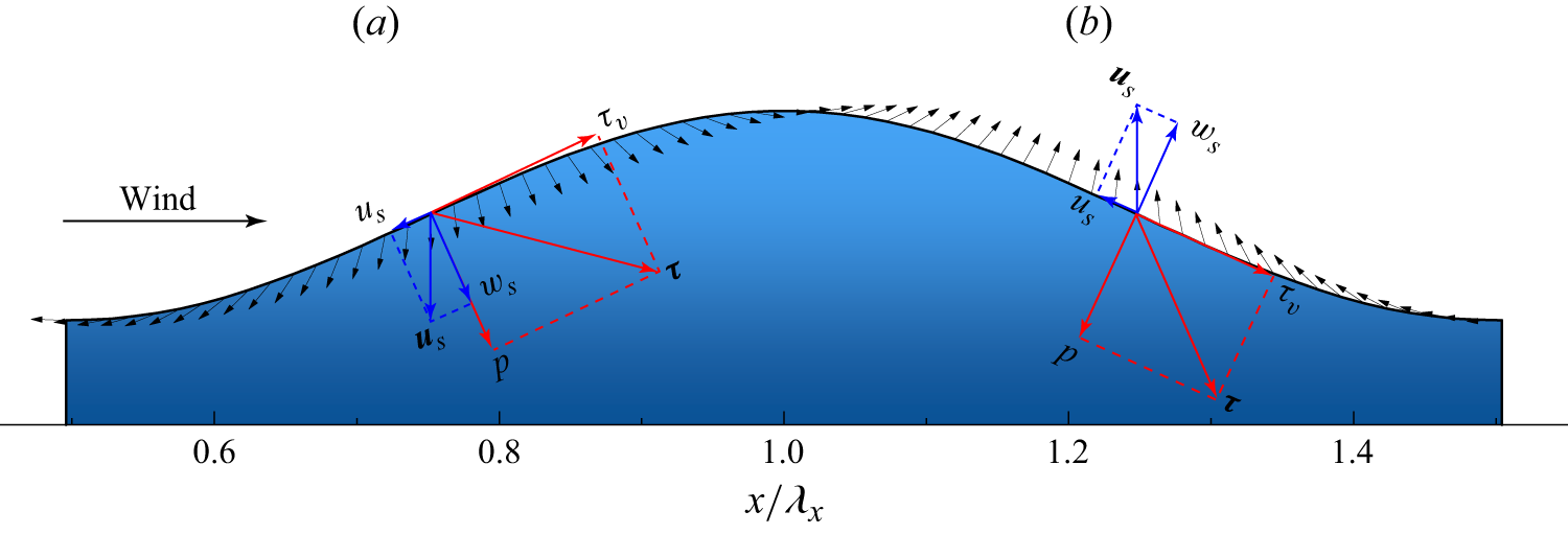
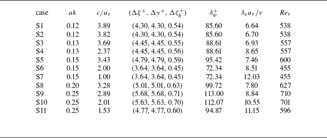
 ak=0.12,0.13,0.15,0.2,0.25
 1.00−3.89
 Re=U0λx/ν≈7300
 U0
 λx
 Reτ=uτλx/ν=455−710
 uτ
 (Δξ+,Δy+,Δζb+)≈(5,5,0.5)
 (ξ,ζ)=(x,(z−η/Hh))
 η
 Hh
 δw+=uτ/kν
 δsuτ/ν
 δs=2ν/ck
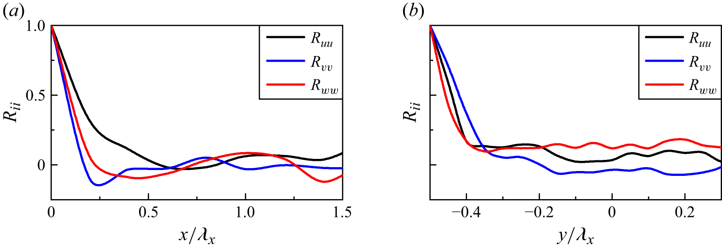
 ζuτ/ν≈80

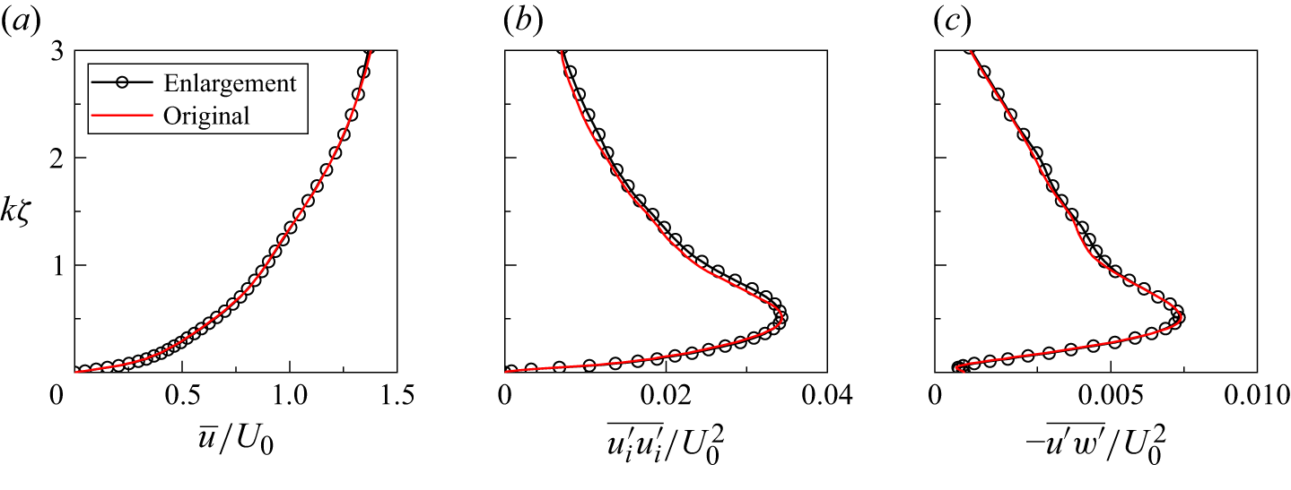
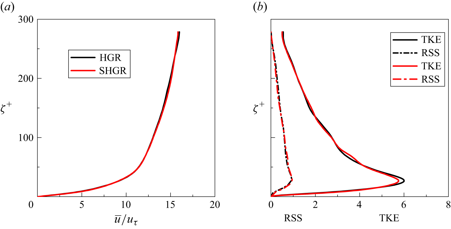

 ak=0.13
 c/uτ=3.69
 ak=0.25
 c/uτ=2
 ak=0.1
 c/uτ=2
 ak=0.1
 c/uτ=3.9
 ak=0.1
 c/uτ=4
 Reτ=200
 Reτ=950
 ak=0.15
 c/uτ=3.46
 Reτ=867
 ak=0.1
 c/uτ=7.25
 Reτ≈3456
 ak=0.14
 c/uτ=7.7
 Reτ=2000
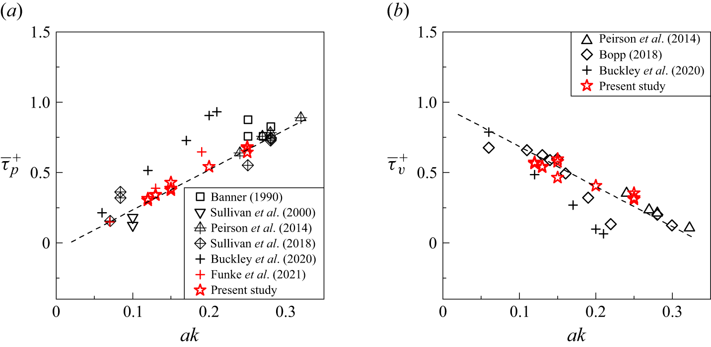
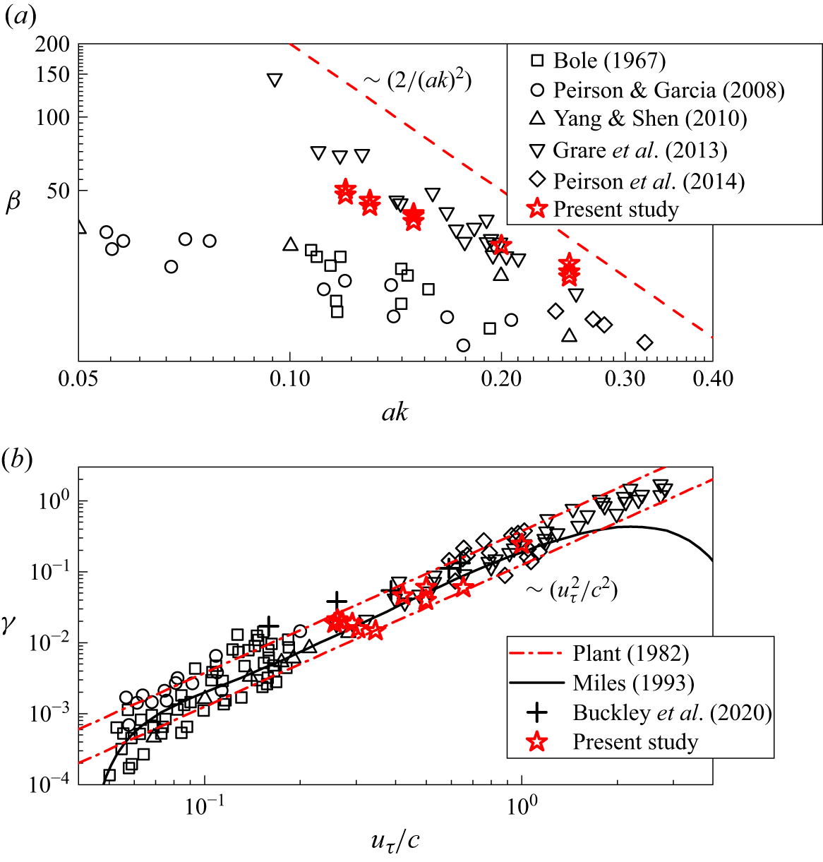
 β
 γ
 γ=2π(0.04±0.02)uτ2/c2
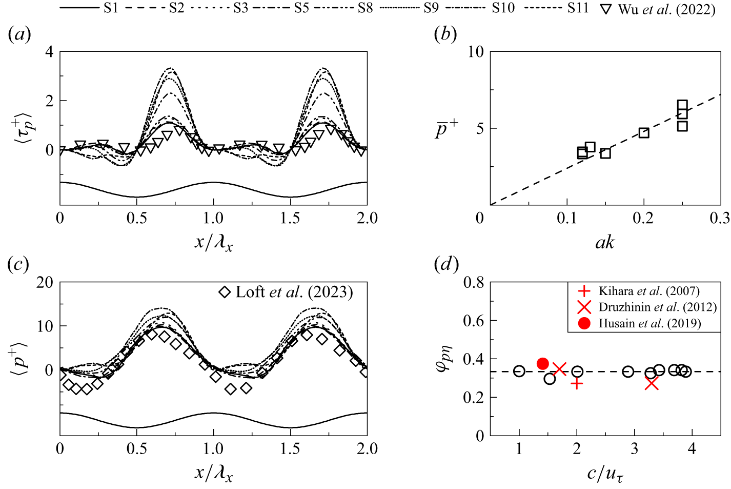
 ak=0.15
 c/uτ=2
 ak=0.09
 c/uτ=6.4


 P=0.2
 Γ=0.02
 νw=0.0009
 2πφpη=0.668π
 γ~
 P=0.3
 Γ=0.03
 νw=0.0009
 2πφpη=0.668π
 γ~
 a1k=0.1

 ak−uτ/c
 ak=0.021(U/c)≈0.714(uτ/c)
 ak=0.35(uτ/c)0.8

 S=3ak
 Pk/ρwg=0.01
 Pk/ρwg=0.5

 S=0.153(U/c)0.3≈0.44(uτ/c)0.3
 U
 S=0.036U/c+0.061≈1.224uτ/c+0.061
 ak=0.35(uτ/c)0.8

 Pk/ρwg=0.01
 Pk/ρwg=0.5
 ak=0.165,0.1,0.05
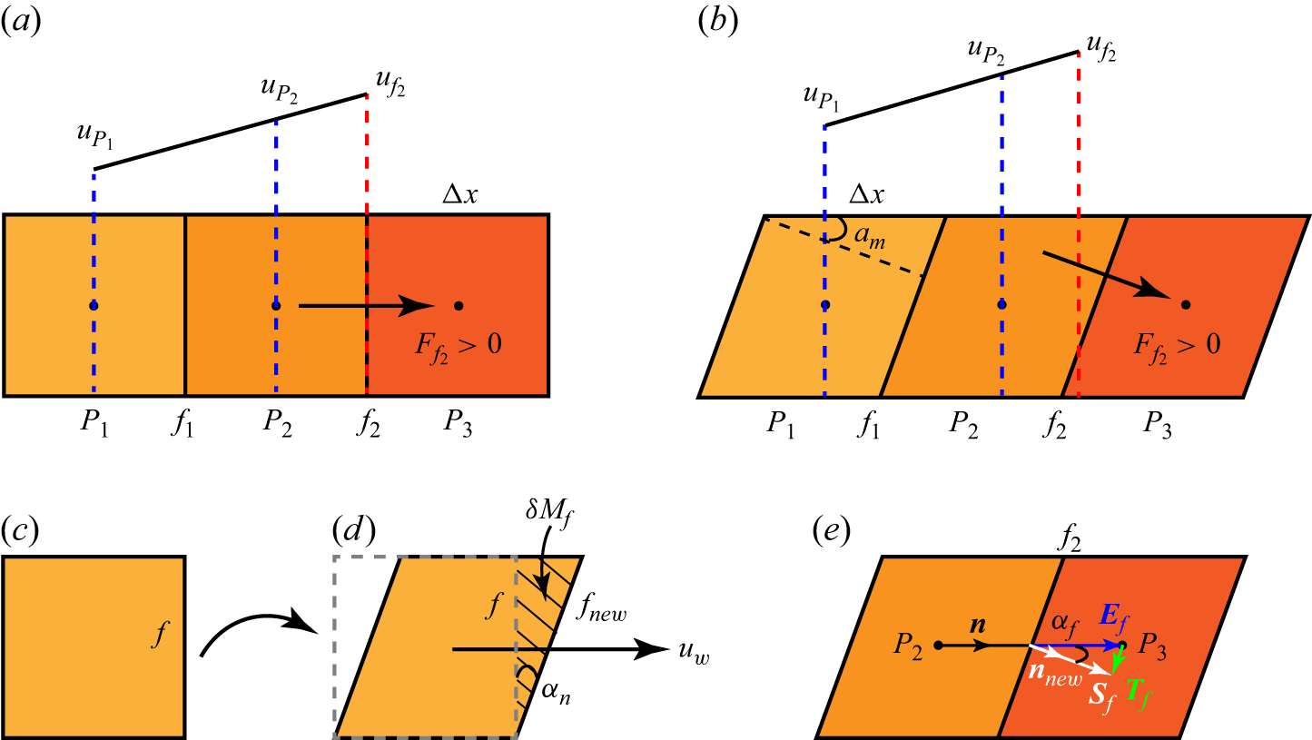
 t
 t+Δt
 δMf
 f

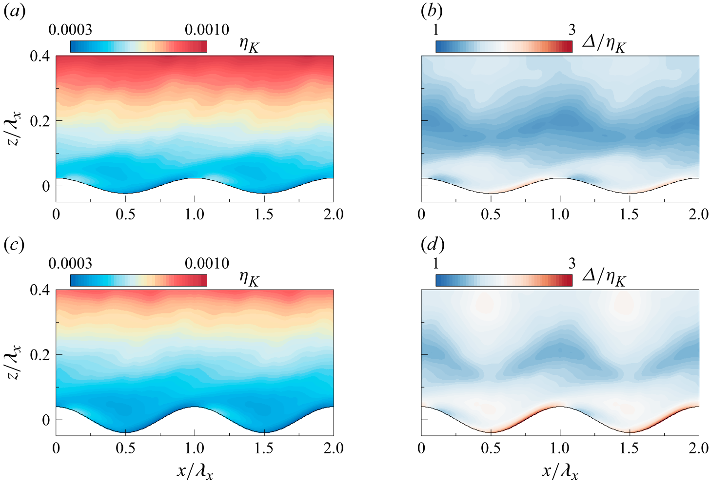
 ηK
 Δ/ηK

 ηK
 Δ/ηK
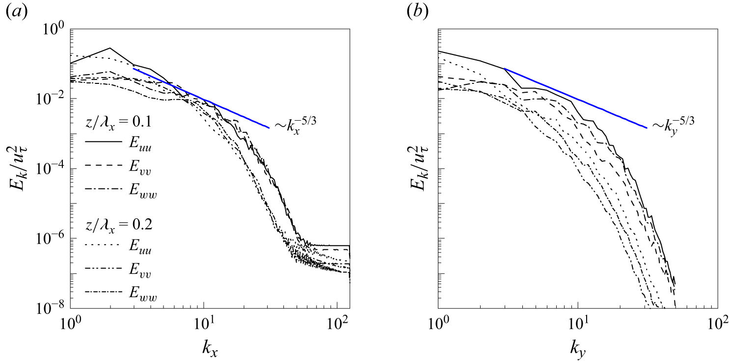
 Ek(kx)/uτ2
 Ek(ky)/uτ2
 z/λx=0.1
 z/λx=0.2
 −5/3

 ak=0.25

 λci=5
 ωx>0
 ωx<0
 −v′+w′+
 uτ2
 x/λx=0.65
 x/λx=1.35



