1 Introduction
This paper concerns the problem of the Simultaneous Localization and Mapping (SLAM) algorithm, which consists of building a map of an unknown environment while the vehicle localizes itself within that map and moves around it. It proposes a scheme enabling the integration of non-reactive control strategies for local or global navigation of a mobile robot in a structured environment while a SLAM algorithm is continuously executed. The SLAM algorithm consists of a sequential EKF (extended Kalman filter) feature-based SLAM. This algorithm fuses corners (convex and concave) and lines of the environment in the SLAM system state. The navigation strategy is based on the construction of uncertainty maps based on the Gaussianity of the SLAM system state and the sum of Gaussians method. The uncertainty maps provide navigation goals and priorities to the navigation strategy, indicating the regions of the environment of which there is no information available. The algorithms and architectures of the proposal, along with real-time experimental results are also shown in this work.
The combination of the SLAM algorithm with a strategy for exploration or navigation within the environment is known as Active SLAM and has been a key problem in the implementation of autonomous mobile robots. The integration of SLAM algorithms with control strategies to govern the motion of a mobile robot and the ability of selecting feasible destinations on its own will endow the vehicle with full autonomy.
In the early development stages of SLAM (Chatila & Laumond, Reference Chatila and Laumond1985; Smith et al., Reference Smith, Self and Cheeseman1987; Ayache & Faugeras, Reference Ayache and Faugeras1989; Smith et al., Reference Smith, Self and Cheeseman1990), the attention of the scientific community is focused on solving the issues inherent to the specification of SLAM schemes: optimality, computational cost and consistency. Several algorithms have been proposed as a result. The EKF (Dissanayake et al., Reference Dissanayake, Newman, Clark, Durrant-Whyte and Csorba2001; Guivant & Nebot, Reference Guivant and Nebot2001; Bailey et al., 2006; Castellanos et al., Reference Castellanos, Neira and Tardos2004; EKF) is one of the first and most used filters to implement a SLAM algorithm, and, among its variants, one may single out the unscented Kalman filter (Thrun et al., Reference Thrun, Burgard and Fox2005), with better performance for nonlinear models and the information filter (Thrun et al., Reference Thrun, Burgard and Fox2005), with better computational performance at the correction stage. More recently, the particle filter (Thrun et al., Reference Thrun, Burgard and Fox2005) and some Bayesian approaches (Thrun et al., Reference Thrun, Burgard and Fox1998; Dellaert et al., Reference Dellaert, Fox and Burgard1999; Hähnel et al., Reference Hähnel, Fox, Burgard and Thrun2003) to SLAM have enabled significant improvements in the SLAM implementation. Unfortunately, most of this research is confined to simulation or off-line results (Huang et al., Reference Huang, Mourikis and Roumeliotis2008; Mullane et al., Reference Mullane, Ba-ngu, Adams and Wijesona2008; Xi et al., Reference Xi, Guo, Sun and Huang2008). In what concerns real-time implementation, the reduction of the computational cost in the execution of SLAM has been achieved through feature-based SLAM with feature selection (di Marco et al., Reference di Marco, Garulli, Lacroix and Vicino2000; Durrant-Whyte & Bailey, Reference Durrant-Whyte and Bailey2006a, 2006b; Auat Cheein et al., Reference Auat Cheein, Scaglia, di Sciascio and Carelli2009b), as well as topological and hybrid maps (Choset & Nagatami, Reference Choset and Nagatani2001; Zunino & Chrinstensen, Reference Zunino and Chrinstensen2001; Garulli et al., Reference Garulli, Giannitrapani, Rosi and Vicino2005). However, in order to reduce processing time, most of the feature-based SLAM applications are restricted to single feature environments (Choset & Nagatami, Reference Choset and Nagatani2001; Durrant-Whyte & Bailey, Reference Durrant-Whyte and Bailey2006b). Finally, the consistency of the SLAM algorithm has been one of the most studied issues in the last years (Zunino & Chrinstensen, Reference Zunino and Chrinstensen2001; Andrade-Cetto & Sanfeliu, Reference Andrade-Cetto and Sanfeliu2002; Kouzoubov & Austin, Reference Kouzoubov and Austin2004; Diosi & Kleeman, Reference Diosi and Kleeman2005; Mullane et al., Reference Mullane, Ba-ngu, Adams and Wijesona2008). This research effort led to the characterization of the sensitivity of SLAM algorithms with respect to its initial conditions and to the Jacobian matrix associated with the environment feature model (Andrade-Cetto & Sanfeliu, Reference Andrade-Cetto and Sanfeliu2002; Diosi & Kleeman, Reference Diosi and Kleeman2005). Fusion of the information on the pose of the mobile robot with data from an external sensor, such as Global Positioning System, is the main approach to maintain the consistency of the SLAM algorithm (Diosi & Kleeman, Reference Diosi and Kleeman2005).
The combination of control strategies with the SLAM algorithm has been addressed from two significantly different points of view. While the first one considers how the control is used to reduce errors during the estimation process (Chatila & Laumond, Reference Chatila and Laumond1985), the second one concerns exploration techniques providing the best map from the reconstruction perspective. Despite the duality between regulation and estimation, whatever the control strategy is implemented, it will not be guaranteed that, in general, the mobile robot will follow a specific trajectory inside the environment (Bailey et al., Reference Bailey, Nieto, Guivant, Stevens and Nebot2006). In many applications, the control signal is not considered as an input of the SLAM algorithm, and, instead, odometry measurements of the robot are used (Thrun et al., Reference Thrun, Burgard and Fox2005; Durrant-Whyte & Bailey, Reference Durrant-Whyte and Bailey2006a, 2006b). Thus, most of the associated implementations focus on the low-level, basic control-reactive behavior (Zunino & Chrinstensen, Reference Zunino and Chrinstensen2001; Diosi & Kleeman, Reference Diosi and Kleeman2005), leaving the motion planning and control as a secondary algorithm. Thus, albeit restricted to a local reference frame attached to the robot, active exploration strategies for indoor environments are proposed by Xi et al. (Reference Xi, Guo, Sun and Huang2008), Andrade-Cetto and Sanfeliu (Reference Andrade-Cetto and Sanfeliu2006) and Liu et al. (Reference Liu, Dong and Sun2008). As an example, a boundary exploration problem is proposed by Xi et al. (Reference Xi, Guo, Sun and Huang2008). In this case, the robot has to reach the best point determined in the boundary of its local point of view. From a global reference perspective, these implementations have a random behavior inside the environment. To solve the lack of global planning, some implementations have included algorithms for searching optimal path based on the information acquired of the environment (Sim & Roy, Reference Sim and Roy2005; Liu et al., Reference Liu, Dong and Sun2008). These algorithms usually require the map to be gridded and, accordingly, they compute a feasible path to a possible destination (closure of the loop or global boundary points) without specifying the control law implemented on the mobile robot. Despite the advances made so far, the integration of control strategies based on the SLAM system state—map and vehicle (Durrant-Whyte & Bailey, Reference Durrant-Whyte and Bailey2006a, 2006b) to guide the robot within an unknown environment from a local and a global reference frame following a preestablished plan is not quite studied or implemented in real time.
The main contribution of this paper is twofold: (1) a general algorithm and uncertainty maps-based navigation strategy for an autonomous SLAM implementation (with non-reactive controllers); and (2) the construction of uncertainty maps based on the Gaussianity of the SLAM system state to determine unvisited regions of the environment—from a probabilistic perspective—guiding the robot to those regions and executing the SLAM algorithm at the same time. The navigation strategy presented in this paper allows the determination of unsatisfactorily mapped or unvisited regions of the environment, which will thus be targeted by the robot and thus permitting the autonomous map improvement. The uncertainty maps construction is based on the sum of Gaussians method and the Monte Carlo method. By using the Monte Carlo method instead of gridding the map, we reduce the computational cost of the process and then, by applying the sum of Gaussians method to the navigable points of the environment, we are able to construct an uncertainty map of such environment.
This paper is completed with an introduction of a general algorithm for a real-time SLAM-Control implementation to avoid inconsistency in the map reconstruction (Andrade-Cetto & Sanfeliu, Reference Andrade-Cetto and Sanfeliu2006). This algorithm uses a prediction of the robot's pose up to the time the control law is invoked. Several experimental results are shown along the paper. All experiments were carried out in real time. Potential applications of the obtained results are surveillance, metric maps reconstruction and the construction of probabilistic maps based on the information of the SLAM system state without gridding the environment. During the entire navigation or exploration phase, the SLAM algorithm continues being executed.
This paper is organized as follows. In Section 2, the sequential EKF feature-based SLAM is presented; Section 3 shows the general algorithm of the SLAM combined with a non-reactive controller; Section 4 shows the general method of constructing uncertainty maps, the sum of Gaussians method and the navigation strategy based on priority levels of uncertainty regions of the map. Each section shows real-time experimental results of their proposal. Finally, Section 5 shows the real-time experimental result of the navigation strategy combined with the uncertainty maps method.
2 Feature-based extended Kalman filter–Simultaneous Localization and Mapping
The SLAM algorithm implemented in this work is solved by an EKF. The SLAM system state is composed of the vehicle estimated pose—position and orientation—and the features extracted from the environment—which are known as the map of the environment. The features extracted from the environment correspond to corners—concave and convex—and lines associated with walls. For visualization and map reconstruction purposes, a secondary map is maintained. This secondary map stores the beginning and ending points of the segments associated with the lines of the environment. Thus, the secondary map allows finite walls’ representation. The secondary map is updated and corrected according to the feature correction in the EKF–SLAM system state, and if a new feature is added to that system state, it is also added in the secondary map (Auat Cheein et al., Reference Auat Cheein, De La Cruz, Carelli and Bastos-Filho2009a). Equations (1) and (2) show the system state structure and its covariance matrix. All elements of the SLAM system state are referenced to a global coordinate system:
 $${{\hat{\xi }}_t}\: = \:\left[ \matrix{ {{{{\hat{\xi }}}_{v,t}}} \cr\ {{{{\hat{\xi }}}_{m,t}}} \\\end{}} \right]$$
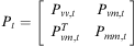 $${{P}_t}\: = \:\left[ \matrix { {{{P}_{vv,t}}} & {{{P}_{vm,t}}} \cr\ {P_{{vm,t}}^{T} } & {{{P}_{mm,t}}} \\\end{}} \right]$$
In Equation (1),  $ {{\hat{\xi }}_t} $ is the SLAM system state;
 $ {{\hat{\xi }}_{v,t}}\: = \:[\matrix { {{{{\hat{\xi }}}_{x,t}}} & {{{{\hat{\xi }}}_{y,t}}} & {{{{\hat{\xi }}}_{\theta, t}}} \\\end{}] $ is the estimated pose of the vehicle, where
 $ {{\hat{\xi }}_{x,t}} $ and
 $ {{\hat{\xi }}_{y,t}} $ represent the global position of the agent within the environment and
 $ {{\hat{\xi }}_{\theta, t}} $ its orientation;
 $ {{\hat{\xi }}_{m,t}} $ represents the map of the environment and it is composed of parameters that define both: lines and corners (corners are defined in the Cartesian space and lines in the polar space as will be shown in Section 2.2). The order in which lines and corners appear in
 $ {{\hat{\xi }}_{m,t}} $ depends on the moment they were detected. Pt is the covariance matrix associated with the SLAM system state; Pvv ,t is covariance of the vehicle's pose and Pmm ,t is the covariance of the map. Pvm ,t and
 $ P_{{mv,t}}^{T} $ are cross-correlation matrices (between the vehicle and the map).
The covariance matrix initialization techniques and the EKF definition can be found in Durrant-Whyte and Bailey (Reference Durrant-Whyte and Bailey2006a). The EKF is represented in Equation (3). All variables involved in the estimation process are considered as Gaussian random variables:
 $$\left\{{ \matrix{ {\hat{\xi }_{t}^{{\rm{ - }}} \: = \:f({{{\hat{\xi }}}_t},{{u}_t})} \hfill \cr\ \!\!{P_{t}^{{\rm{ - }}} \: = \:{{A}_t}{{P}_{t{\rm{ - }}1}}A_{t}^{T} \: + \:{{W}_t}{{Q}_{t{\rm{ - }}1}}W_{t}^{T} } \hfill \cr\ \!\!{{{K}_t}\: = \:P_{t}^{{\rm{ - }}} H_{t}^{T} {{{({{H}_t}P_{t}^{{\rm{ - }}} H_{t}^{T} \: + \:{{R}_t})}}^{{\rm{ - }}1}} } \hfill \cr\ \!\!{{{{\hat{\xi }}}_t}\: = \:\hat{\xi }_{t}^{{\rm{ - }}} \: + \:{{K}_t}({{z}_t}{\rm{ - }}h(\hat{\xi }_{t}^{{\rm{ - }}} ))} \hfill \cr\ \!\!{{{P}_t}\: = \:(I{\rm{ - }}{{K}_t}{{H}_t})P_{t}^{{\rm{ - }}} .} \hfill \\\end{}} \right$$
In Equation (3),  $ \hat{\xi }_{t}^{{\rm{ - }}} $ is the predicted state of the system at time t; ut is the input control commands and
 $ \hat{\xi }_{t}^{{}} $ is the corrected state at time t; f describes the motion of the elements of
 $ \hat{\xi } $.
 $ P_{t}^{{\rm{ - }}} $ and Pt are the predicted and corrected covariance matrices, respectively, at time t; At is the Jacobian of f with respect to the SLAM system state and Qt is the covariance matrix of the noise associated with the process, whereas Wt is its Jacobian matrix; Kt is the Kalman gain at time t; Ht is the Jacobian matrix of the measurement model (h) and Rt is the covariance matrix of the actual measurement (zt). The term
 $ ({{z}_t}{\rm{ - }}h(\hat{\xi }_{t}^{{\rm{ - }}} )) $ is called the innovation vector (Thrun et al., Reference Thrun, Burgard and Fox2005) and takes place when the data association procedure has reached an appropriate matching between the observed feature and the predicted one
 $ (h(\hat{\xi }_{t}^{{\rm{ - }}} )) $. Both the process model (f) and the observation model are nonlinear expressions. Further information about the EKF–SLAM can be found in Auat Cheein et al. (Reference Auat Cheein, De La Cruz, Carelli and Bastos-Filho2009a).
In this work, the sequential EKF was implemented in order to reduce computational costs. The sequential EKF–SLAM is based on the iterative calculation of the correction stage (SLAM system state and covariance matrix) for each feature with correct association—see Thrun et al. (Reference Thrun, Burgard and Fox2005). The last statement implies that the Jacobian matrix of the measurement model and Kalman gain are sparse matrices, decreasing in that way the processing time during a correction iteration. Nevertheless, the prediction stage remains as stated in Equation (3).
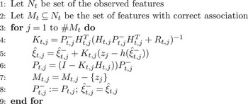
The general form of the correction stage of the classical sequential EKF–SLAM algorithm (Thrun et al., Reference Thrun, Burgard and Fox2005) is summarized in the algorithm shown in Figure 1. Sentences (3) to (9) describe the for-loop of the correction stage of the algorithm. For every feature with correct association—sentence (2)—the for-loop is executed. Sentence (4) shows the Kalman gain calculation; sentence (5) is the correction of the SLAM system state, whereas sentence (6) is the correction of the covariance matrix of the SLAM algorithm; in sentence (7), the current feature is deleted from the set of features with correct association (Mt). In the next iteration, the next predicted SLAM system state and covariance matrix are the last corrected SLAM system state and covariance matrix, respectively, as noted in sentence (8).
Algorithm of the correction stage of the Sequential extended Kalman filter–Simultaneous Localization and Mapping

Further information concerning the EKF–SLAM implemented in this work can be found in Auat Cheein et al. (Reference Auat Cheein, Toibero, Lobo Pereira, di Sciascio and Carelli2010).
2.1 Mobile robot
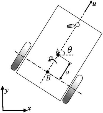
The vehicle used in this work is a non-holonomic unicycle type mobile robot Pioneer 3AT built by ActivMedia. Figure 2 shows the kinematic model of the mobile robot. Equation (4) shows the discrete kinematic equation of the robot:
Graphic representation of the kinematic model of the unicycle mobile robot

 $${{\left[ {\matrix{ {{{\xi }_{x,t}}} \cr\ {{{\xi }_{y,t}}} \cr\ {{{\xi }_{\theta, t}}} \\\end{}}} \right]}_G}\, = \,\left[ {\matrix {{{{\xi }_{x,t{\rm{ - }}1}}} \cr\ {{{\xi }_{y,t{\rm{ - }}1}}} \cr\ {{{\xi }_{\theta, t{\rm{ - }}1}}} \\\end{}}} \right]\, + \,\rDelta t\left[ \matrix{ {\cos ({{\xi }_{\theta, t{\rm{ - }}1}})} & {{\rm{ - }}a\sin ({{\xi }_{\theta, t{\rm{ - }}1}})} \cr{\sin ({{\xi }_{\theta, t{\rm{ - }}1}})} & {a\cos ({{\xi }_{\theta, t{\rm{ - }}1}})} \cr\ 0 & 1 \\\end{}} \right]\left[ \matrix { {{{u}_t}} \cr\ {{{\omega }_t}} \\\end{}}} \right]\, + \,{{\rPhi }_t}$$
In Equation (4), ξx ,t, ξy ,t and ξθ ,t are the coordinates of h—the point of control of the mobile robot—in Figure 2; Φt is the discrete time Gaussian process noise associated with the robot's model; ut is the linear velocity command applied to the vehicle and ωt is the angular velocity command; Δt is the sampling time of the system. The suffix G in Equation (4) refers that the coordinates of the mobile robot are expressed in a global reference frame of the environment.
2.2 Features of the environment
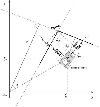
The models of the features of the environment—corners and lines—are shown in Equations (5) and (6). Figure 3 shows the graphical interpretation of the variables in Equations (5) and (6). Although all features are extracted from a local reference frame attached to the mobile robot, they are added to the SLAM system state once their parameters are converted to the global reference frame of the system (Durrant-Whyte & Bailey, Reference Durrant-Whyte and Bailey2006a).
Graphic representation of line and corners extracted from the environment

 $$\matrix {{ & {{z}_{corner}}(k)\: = \:{{h}_i}[{{{\hat{\xi }}}_{v,t}},w(k)]\: = \:\left[ \matrix {{{{z}_R}} \cr\ {{{z}_\beta }} \\\end{}} \right]} = \cr\ {\left[ {\matrix{ \sqrt {{{{({{ {\hat{\xi }}}_{x,t}}(k){\rm{ - }}{{x}_{corner}})}}^2} \, + \,{{{({{{\hat{\xi }}}_{x,t}}(k){\rm{ - }}{{y}_{corner}})}}^2} } \cr\ \arctan \frac{{{{{\hat{\xi }}}_{y,t}}(k){\rm{ - }}{{y}_{corner}}}}{{{{{\hat{\xi }}}_{x,t}}{\rm{ - }}{{x}_{corner}}}}{\rm{ - }}{{{\hat{\xi }}}_{\theta, t}}(k) \\ \end{}}} \right]}\ \cr\ { & + \left[ \matrix { {{{w}_R}} \cr\ {{{w}_\beta }} \\\end{}} \right]} \\\end{}$$
 $$\matrix {{ & {{z}_{line}}(k)\: = \:{{h}_i}[{{{\hat{\xi }}}_{v,t}},w(k)]} = \cr\ {\left[ \matrix { {{{Z}_\rho }} \cr\ {{{Z}_\alpha }} \\\end{}} \right]\, = \,\left[ \matrix { {r\,{\rm{ - }}\,{{{\hat{\xi }}}_{x,t}}(k)\cos (\alpha )\,{\rm{ - }}\,{{{\hat{\xi }}}_{v,t}}(k)\sin (\alpha )} \cr\ {\alpha \,{\rm{ - }}\,{{{\hat{\xi }}}_{\theta, t}}(k)} \\\end{}} \right]} \cr\ { & + \left[ \matrix {{{{w}_\rho }} \cr\ {{{w}_\alpha }} \\\end{}} \right]} \\\end{}}$$
In Equations (5) and (6), wρ, wα, wR, wβ are additive Gaussian noise associated with the measurement. Further information concerning the line's modeling can be found in Garulli et al. (Reference Garulli, Giannitrapani, Rosi and Vicino2005). The corners’ extraction method can be seen in Guivant and Nebot (Reference Guivant and Nebot2001).
3 Simultaneous Localization and Mapping-Control algorithm: implementation issues
The combination of a control strategy—for navigation purposes—within the SLAM algorithm provides the mobile robot with full autonomy (Thrun et al., Reference Thrun, Burgard and Fox2005). The control strategy can be divided into two: reactive and non-reactive—or planned—control.
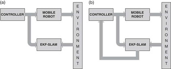
The reactive control strategy is usually implemented on a behavior-based case strategy—or sensor-based navigation. The mobile robot does not need its pose information to plan its movements beyond a local reference frame attached to the vehicle (Arkin, Reference Arkin1998)—which is usually accomplished with odometry measurements due to the fact that for small distances, the variance of the odometry can be discarded (Thrun et al., Reference Thrun, Burgard and Fox2005). Thus, there is no communication between the SLAM and the control strategy. This kind of SLAM-Control architectures are developed for exploration tasks. Whether the SLAM becomes inconsistent or not does not affect the exploration. The SLAM-Reactive Control strategy is represented in Figure 4(a).
Schematic of the Simultaneous Localization and Mapping (SLAM) algorithm combined with control. (a) Shows the SLAM with reactive control, the SLAM does not return any information to the controller; (b) shows the SLAM with non-reactive control, the controller uses the robot's pose estimated by the SLAM algorithm in order to update the control references. EKF = extended Kalman filter

On the other hand, when the SLAM is combined with a plan-based control strategy—such as trajectory or path following controller—the control needs the robot's current pose in order to calculate the references and the control actions. Thus, for a stable control law if the SLAM turns into inconsistency, the control will remain stable, although the objective of the navigation will not be fulfilled because of erroneous references—if the SLAM turns into inconsistency, then the estimation is no longer reliable. Furthermore, due to the non-constant time of the SLAM's executions (Thrun et al., Reference Thrun, Burgard and Fox2005), the stability of the controller can also be compromised (the controller must be stable for non-constant sampling time). Thus, not any controller can be implemented within a SLAM algorithm. As it can be seen, the SLAM algorithm with non-reactive controllers is more sensitive to the SLAM performance than with reactive controllers. Figure 4(b) shows the general architecture of an autonomous SLAM with non-reactive control strategy.
Beyond the control stability issues, the fact of the SLAM algorithm being not constant time also compromises the mobile robot integrity. Considering that all inner parameters of the robot are set up every sampling time, that is, if the control input changes at a time between time t and t + t 1, it will be effective only in time t + t 1, let us suppose the following scenario: the SLAM algorithm is executed at time t and it ends at time t + Δ, with Δ > 0. In an implementation of the SLAM-Control algorithm, if during the interval [t, t + Δ] there was a change in the motion commands, they will not be effective until the next sampling time following t + Δ (let us call it t + tk, where tk ⩾ Δ). The last sentence implies that during the Δ-time, the robot was in an open loop situation. Furthermore, after the t + Δ time, the estimation of the pose will correspond to the pose that the vehicle had at instant t and that information is then passed to the controller. Thus, the controller at time instant t + tk will have the references of instant t. The last statement also implies a limitation in the velocity of the robot: if the robot is navigating in an open loop situation, it could collide. In order to avoid this open loop situation, a predictor is used in this work. The following section shows the implementation of a control architecture encompassing a predictor, SLAM, and a reactive controller. By using a predictor during the open loop situation, there will be available information concerning the current pose of the vehicle in the corresponding SLAM calculations.
A last remark is necessary. If the SLAM-Control algorithm is implemented as a sequential algorithm, the control commands can be changed only at the next sampling time after the last SLAM execution.
3.1 Sequential algorithm structure
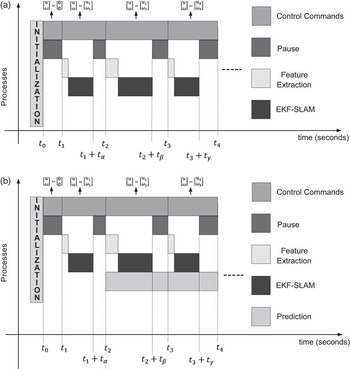
The time charts shown in Figure 5 shows the sequential implementation of the SLAM algorithm. As recommended by Durrant-Whyte and Bailey (Reference Durrant-Whyte and Bailey2006b), before the mobile robot's initial motion, it extracts the first features from the environment. In this way, once the navigation cycle is closed, the final covariance matrix of the SLAM system state will tend to its initial values.
Chart time of the Simultaneous Localization and Mapping (SLAM)-Control implementation. (a) Shows the SLAM-Control implementation without a predictor and (b) shows the chart time of a SLAM-Control implementation with a predictor

Figure 5(a) shows an SLAM-Control implementation without a predictor, whereas Figure 5(b) shows the sequential implementation of the SLAM-Control with a predictor. As it can be seen in Figure 5, a cycle of the SLAM-Control algorithm is composed of three stages: Features Extraction–SLAM–Pause, in that order. Thus, after the robot's initialization, it extracts the features from the environment. After the features extraction, the SLAM is performed. Both, the corrected SLAM system state and covariance matrix are used to calculate the control commands of the mobile robot. Then, in order to update the mobile robot parameters, a pause is needed between the SLAM ending and the following sampling time of the robotic system. During this pause, the robot continues its motion according to its previous command controls.
Regarding the SLAM-Control implementation, let us consider Figure 5(a) and let Δ be the sampling time of the system—Δ not necessarily constant. Thus,
1. After the initialization of the system, the control commands of the mobile robot are set up to zero: [u ω]T = [0 0]T and they are effective after the first pause, that is, at instant time t 1.
2. From instant time t 1 up to t 2, the control command remains unchanged.
3. At time t 1 + tα, with α ⩽ Δ, a new features extraction and SLAM process are completed. Based on the information provided by the SLAM system state and its covariance matrix, the next mobile robot control commands are generated ([u ω]T = [v 1ω 1]T), where they will be effective only at time t 2 (because of the necessary pause of the system) and maintained up to time t 3. Let us recall that the SLAM system state and covariance matrix estimation at time t 1 + tα corresponds to the robot's pose at time t 1.
4. At time t 2, the mobile robot motion is set up to [u ω]T = [u 1ω 1]T. A features extraction and a SLAM execution are processed.
5. At time t 2 + tβ, with tβ ⩽ Δ, a new estimation of the system state is available from the SLAM algorithm and new control commands are generated based on that information ([v ω]T = [u 2ω 2]T). The new control commands will only be effective at t 3, meanwhile, the current control commands correspond to [u ω]T = [u 1ω 1]T.
6. The process repeats successively.
Thus, in the chart shown in Figure 5(a), no predictor is used. Due to the fact that the control commands are generated based on a past value of the mobile robot's pose, this situation could lead to inconsistency of the map, as will be shown in Section 3.2. This is so because the covariance matrix associated with the control errors—Qt in Equation (3)—cannot absorb the errors of the robot's pose as the SLAM algorithm execution time increase.
In the chart shown in Figure 5(b), the sequential SLAM-Control implementation is presented. In this chart, a prediction stage is used in order to compensate the lack of robot's pose information present in the chart of Figure 5(a). The SLAM-Control functionality is similar to the one presented before, with the following differences:
1. At time t 2 + tβ, the control commands—[u 2ω 2]—are generated based on the information provided by the SLAM system state and its covariance matrix and the predicted pose of the mobile robot with the current control commands ([u ω]T = [u 1ω 1]T). Thus, the predicted pose concerns the elapsed time between t 2 and t 2 + tβ. The control commands [u 2ω 2] will be effective at time instant t 3.
2. The control commands at time t 3 + tγ are generated based on the information provided by the SLAM system state and its covariance matrix and the prediction of the mobile robot's pose at time t 3 + tγ. The prediction is formed by the elapsed time of the pause of the previous SLAM-Control execution (it is the time between t 2 + tβ and t 3) and the time consumed by the features extraction and the SLAM processes (from t 3 to t 3 + tγ). As it can be seen, from t 2 + tβ to t 3, the mobile robot motion was governed by [u ω]T = [u 1ω 1]T; whereas from time t 3 to t 3 + tγ, the motion commands were [u ω]T = [u 2ω 2]T. Thus, a prediction for both cases is needed.
3. The process repeats successively.
As it can be seen, the control commands in the sequential SLAM-Control implementation are only refreshed after the features extraction and the SLAM process’ endings. The predictor used in this work is presented in Equation (7), which is the same as the one used by the EKF–SLAM algorithm (Auat Cheein et al., Reference Auat Cheein, De La Cruz, Carelli and Bastos-Filho2009a).
 $${{\left[ \matrix { {{{{\hat{\xi }}}_{x,t}}} \cr\ {{{{\hat{\xi }}}_{y,t}}} \cr\ {{{{\hat{\xi }}}_{\theta, t}}} \\\end{}} \right]}_G}\, = \,\left[ \matrix { {{{{\hat{\xi }}}_{x,t{\rm{ - }}1}}} \cr\ {{{{\hat{\xi }}}_{y,t{\rm{ - }}1}}} \cr\ {{{{\hat{\xi }}}_{\theta, t{\rm{ - }}1}}} \\\end{}} \right]\, + \,\rDelta t\left[ \matrix { {\cos ({{{\hat{\xi }}}_{\theta, t{\rm{ - }}1}})} & {{\rm{ - }}a\sin ({{{\hat{\xi }}}_{\theta, t{\rm{ - }}1}})} \cr{\sin ({{{\hat{\xi }}}_{\theta, t{\rm{ - }}1}})} & {a\cos ({{{\hat{\xi }}}_{\theta, t{\rm{ - }}1}})} \cr\ 0 & 1 \\\end{}} \right]\left[ \matrix { {{{u}_t}} \cr \ {{{\omega }_t}} \\\end{}} \right]$$
In Equation (7), Δt is the elapsed time used for the prediction. Thus, for the case shown in the chart of Figure 5(b), that time could be either tβ, t 3−(t 2 + tβ) or tγ. For example, for Δt = tβ, the prediction equation would be of the form shown in Equation (8).
 $${{\left[ \matrix { {{{{\hat{\xi }}}_{x,{{t}_2}\: + \:{{t}_\beta }}}} \cr\ {{{{\hat{\xi }}}_{y,{{t}_2}\: + \:{{t}_\beta }}}} \cr\ {{{{\hat{\xi }}}_{\theta, {{t}_2}\: + \:{{t}_\beta }}}} \\\end{}} \right]}_G}\, = \,\left[ \matrix{ {{{{\hat{\xi }}}_{x,{{t}_2}}}} \cr\ {{{{\hat{\xi }}}_{y,{{t}_2}}}} \cr\ {{{{\hat{\xi }}}_{\theta, {{t}_2}}}} \\\end{}} \right]\, + \,{{t}_\beta }\left[ \matrix {{\cos ({{{\hat{\xi }}}_{\theta, {{t}_2}}})} & {{\rm{ - }}a\sin ({{{\hat{\xi }}}_{\theta, {{t}_2}}})} \cr{\sin ({{{\hat{\xi }}}_{\theta, {{t}_2}}})} & {a\cos ({{{\hat{\xi }}}_{\theta, {{t}_2}}})} \cr\ 0 & 1 \\\end{}} \right]\left[ \matrix{ {{{u}_1}} \cr\ {{{\omega }_1}} \\\end{}} \right]$$
3.2 Experimental comparisons
For purposes of showing the differences of using a predictor in a SLAM-Control implementation, some real-time experimentations were carried out at the facilities of the Instuto de Automatica, National University of San Juan, Argentina. The mobile robot used was a Pioneer 3AT, introduced in Section 2.1; the features extracted from the environment were lines associated with walls and corners (see Section 2.2); the range sensor used was a laser built by SICK, which acquires 181 measurements in a range of 32 m from 0° to 181°; the EKF–SLAM implemented was presented in Section 2. No odometry information of the robot was included in the estimation process.
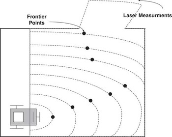
Considering that the objective is to show the advantages of using a predictor within the SLAM-Control algorithm, the navigation strategy was a simple trajectory following based on frontier points determination (Auat Cheein et al., Reference Auat Cheein, De La Cruz, Carelli and Bastos-Filho2009a). Briefly, the frontier points strategy finds non-occupied points of the navigable space at the limit of the sensor range and directs the robot's movements to that point by generating a kinematically plausible path from the robot's position to the frontier point. Also, it is possible to find several frontier points by varying the range of the sensor. Figure 6 shows how successive frontier points are determined. Once the plausible path is found, a kinematic controller drives the robot motion through that path until the robot reaches the frontier point. Once the robot reaches a neighborhood of the frontier point, a new frontier point is determined. This situation repeats until the navigation is interrupted. The kinematic controller implemented in these experiments is the Kanayama's trajectory follower (Kanayama et al., Reference Kanayama, Kimura, Miyazaki and Noguchi1990).
Frontier points determination. The frontier points are determined by localizing middle free space points from the measurement data

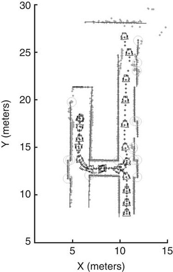
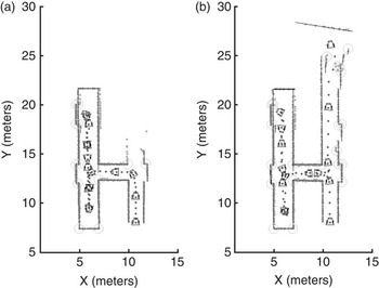
Figure 7 shows the SLAM-Control implementation using the predictor to improve the open loop situation of the navigation during the control planning process. On the other hand, Figure 8 shows two different snapshots at times ta and tb of a same experiment of SLAM-Control algorithm without the predictor. As it can be seen, the map reconstruction starts to become inconsistent at position [x y]T = [12 25]T. A third snapshot after tb is not presented because the estimation is lost due to the inconsistency and no map can be recovered.
Map reconstruction of the facilities of the Instituto de Automatica. The grey points are raw laser data; the solid black segments represent walls from the environment; light grey circles are corners; and the solid black dotted line is the path traveled by the mobile robot

Two snapshots of a SLAM-Control implementation without a predictor for the planning purpose. (a) Shows the map reconstruction for instant time ta<tb. On the other hand, (b) shows that, at position [x y]T = [25 12]T, the map starts to differ from the one shown in Figure 7. The grey points are raw laser data; dotted black line is the path traveled by the mobile robot; segments associated with walls from the environment are represented by solid black lines; and light grey circles are corners—convex and concave

4 Autonomous Simultaneous Localization and Mapping: an uncertainty maps navigation example
In this section, we show an autonomous-driven SLAM example. The mobile robot, while performing the SLAM algorithm, will use information contained within the SLAM system state and its covariance matrix to generate uncertainty maps of the environment. These maps are then used to determine uncertainty zones and the robot is driven to these zones by means of a non-reactive controller. Thus, the vehicle navigates the environment based on the SLAM information, which is recursively updated during navigation.
For the purpose of obtaining uncertainty maps of the environment, a Monte Carlo points generation combined with the sum of Gaussians method for the uncertainty maps construction is proposed in this work. The fact of using the Monte Carlo points generation combined with the sum of Gaussians method substantially decreases the computational costs when compared with a map-gridding procedure (Sanchez Miralles & Sanz Bobi, Reference Sanchez Miralles and Sanz Bobi2004; Thrun et al., Reference Thrun, Burgard and Fox2005).
4.1 Monte Carlo uncertainty maps building procedure
The construction procedure of the uncertainty maps can be summarized as follows:
1. The geometrical representation of the map built by the SLAM and the robot's pose are circumscribed by a rectangle. The rectangle is composed of four edges, which are considered as virtual features of the environment.
2. The four virtual features are parameterized as it is shown in Equation (6) and they will be considered as Gaussian distribution functions with probability value of 0.5 at their mean values. By the linear nature of the EKF, the real features of the environment are also Gaussian distributions with mean values given by the SLAM system state and covariance matrix extracted from the SLAM system state covariance matrix. The probability function distribution of the segments of the environment will be explained in detail in Section 4.1.4.
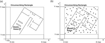
3. Within the space circumscribed by the rectangle, M points are uniformly generated by the Monte Carlo method, covering the mapped space see Figure 9.
Figure 9Monte Carlo points generation procedure. (a) The mapped area and the robot's pose are circumscribed by the rectangle—black solid line and (b) over the circumscribed area, M Monte Carlo points are generated—black dots

4. From the set of M Monte Carlo points, only the navigable points (represented by the set N, where
$ N\: \subseteq \:M $) will be used in the uncertainty points determination.5. Each element of N—the set of navigable points—has a probability value associated with it. That probability is the result of several probability distribution functions associated with each feature of the environment contained within the SLAM system state. Those points whose probability values are near zero will be considered as free space points; those points with probability near one will be considered as occupied points of the environment (e.g., points near walls); and those points whose probability is in a neighborhood of 0.5 will be considered as uncertainty points because no conclusions can be made about the point being occupied or unoccupied. In order to fusion the probability value of a point with respect to the features of the environment, the sum of Gaussians method is performed.
6. The final map is a representation of the probability values associated with the navigable points of the mapped environment.


The following subsections will show the Monte Carlo uncertainty maps construction in detail.
4.1.1 Monte Carlo points generation
In order to present the Monte Carlo points generation, let us suppose the map shown in Figure 8 with the circumscribing rectangle in solid red. The mobile robot is positioned within the environment. Furthermore, let Xmax and Ymax be the maximum values circumscribed by the rectangle and Xmin and Ymin the corresponding minimum values referenced to the global reference system used by the SLAM algorithm. Then, the Monte Carlo generation points can be expressed as stated in Equations (9) and (10).
 $$\openup 3pt\left\{ \matrix { {{{\mu }_i}\:\sim \:U({{\lambda }_0},{{\lambda }_1}), \ i\: = \:1, \ldots, M} \hfill \cr\ \!\!{{{m}_i}\: = \:{{X}_{min}}\: + \:({{X}_{max}}{\rm{ - }}{{X}_{min}})\:\times \:{{\mu }_i}} \hfill \\\end{}} \right.$$
 $$\openup 3pt\left\{ \matrix {{{{\mu }_j}\: \sim \:U({{\lambda }_0},{{\lambda }_1}),\ j\: = \:1, \ldots, M} \hfill \cr\ \!\!{{{m}_j}\: = \:{{Y}_{min}}\: + \:({{Y}_{max}}{\rm{ - }}{{Y}_{min}})\:\times \:{{\mu }_j}} \hfill \\\end{}} \right.$$
In Equation (9), μi is the ith outcome of the Monte Carlo experiment (U(λ 0, λ 1) means an uniform distribution with parameters λ 0 = 0 and λ 1 = 1) from a set of M possible points; mi is the x-coordinate (bounded by Xmax and Xmin). Equivalent definitions apply for Equation (10), except that mj is the y-coordinate (bounded by Ymax and Ymin). Thus, the Monte Carlo point generated over the circumscribed space shown in Figure 9(a) is expressed as  $ [x\,y]_{{ \lt G \gt }}^{T} \: = \:[{{m}_i}\,{{m}_j}]_{{ \lt G \gt }}^{T} $. Figure 9(b) shows the Monte Carlo generated points for the map shown in Figure 9(a).
4.1.2 Navigable points determination
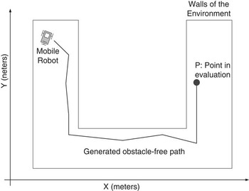
A possible way to check whether a point of a map is navigable or not is to verify that there is an obstacle-free path between the robot and that point. Although several works can be found in the scientific literature to check whether a point is navigable (Arkin, Reference Arkin1998), in this work a metric map-based path generation was implemented. This algorithm consists of generating an obstacle-free path having into account the metric information available in the stored map of the environment. Figure 10 shows an example of the path found by the algorithm that proves the point P within the environment can be reached. The navigable points test is performed over the set M defined above. The set  $ N, N\: \subseteq \:M $ of navigable points will be the set of points for which an obstacle-free path, starting at the robot's pose and ending at the point's location, can be found.
Navigable points determination. If an obstacle-free path can be determined from the mobile robot's pose to the Monte Carlo point P, then P is a navigable point

4.1.3 Probability of a navigable point with respect to a corner
As stated before, the distribution function of any feature extracted from the environment is a Gaussian distribution of the form shown in Equation (11), due to the Gaussianity nature of the EKF. In Equation (11), the mean values ( $ {{[{{\hat{\xi }}_i}\ {{\hat{\xi }}_j}]}^T} $) are extracted directly from the EKF–SLAM system state, where
 $ {{\hat{\xi }}_i} $ corresponds to the random variable at the ith position. The covariance matrix—
 $\rPsi$i—associated with
 $ {{[{{\hat{\xi }}_i}\ {{\hat{\xi }}_j}]}^T} $ is extracted from the EKF–SLAM system state covariance matrix. Thus, if
 $ {{\hat{\xi }}_i} $ and
 $ {{\hat{\xi }}_j} $ are two consecutive variables, their covariance matrix correspond to a 2 × 2 principal sub-matrix located at the ith row, ith column and extended to the jth row, jth column.
Let px ,y = [px py]T be a navigable point of the space and  $ {{[{{\hat{\xi }}_{corner,x}}\ {{\hat{\xi }}_{corner,y}}]}^T} $ the estimated parameters of a corner from the SLAM system state, then the probability of px ,y with respect to the corner can be expressed as
 $$P({{p}_{x,y}})\: = \:\frac{1}{{\sqrt {{{{(2\pi )}}^2} |{{{\rm{\rPsi }}}_i}|} }}{{e}^{{\rm{ - }}\frac{{\rm{1}}}{{\rm{2}}}{{{\left( {\left[ \matrix {{{{p}_x}} \cr\ {{{p}_y}} \\\end{}} \right]{\rm{ - }}\left[ \matrix { {{{{\hat{\xi }}}_{corner,x}}} \cr\ {{{{\hat{\xi }}}_{corner,y}}} \\\end{}} \right]} \right)}}^T} \rPsi _{i}^{{{\rm{ - }}1}} \left( {\left[ \matrix { {{{p}_x}} \cr\ {{{p}_y}} \\\end{}} \right]{\rm{ - }}\left[ \matrix { {{{{\hat{\xi }}}_{corner,x}}} \cr\ {{{{\hat{\xi }}}_{corner,y}}} \\\end{}} \right]} \right)}} $$
Considering that in this work, a corner is modeled in Cartesian coordinates and a line is modeled in the polar coordinate, see Section 2.2, in order to express the probability of a given point with respect to a feature over the same space some transformations are needed, this situation is necessary to apply the sum of Gaussians method. Thus, by applying the Fundamental Probability Theorem (Theodoridis & Koutroumbas, Reference Theodoridis and Koutroumbas2003) to Equation (11), we can obtain the probability of a navigable point px ,y with respect to a corner in the polar space instead of the Cartesian space. Thus, let ƒ(σ, τ) be a density probability function defined in the polar coordinate system. Also, let gσ(x, y) = σ and hτ(x, y) = τ be two functions that relate Cartesian coordinates x and y with σ and τ from the polar coordinate system, where σ is related to the distance to the origin of the system and τ is its angle. Then,
 $$\matrix { {f(\sigma, \tau )\: = \:\frac{{f(x,y)}}{{|J(x,y)|}}} \cr\ {|J(x,y)|\: = \:\left| \matrix { {\frac{{\partial \sigma }}{{\partial {{p}_x}}}} & {\frac{{\partial \sigma }}{{\partial {{p}_y}}}} \cr\ {\frac{{\partial \tau }}{{\partial {{p}_x}}}} & {\frac{{\partial \tau }}{{\partial {{p}_y}}}} \\\end{}} \right|\, = \,{{{\left| \matrix { {\frac{{\partial {{p}_x}}}{{\partial \sigma }}} & {\frac{{\partial {{p}_y}}}{{\partial \sigma }}} \cr\ {\frac{{\partial {{p}_x}}}{{\partial \tau }}} & {\frac{{\partial {{p}_y}}}{{\partial \tau }}} \\\end{}} \right|}}^{{\rm{ - }}1}} } \\\end{}$$
where J is the Jacobbian matrix associated with the transformation. Applying the equations above to transform Equation (11) into the polar space we have that
 $$\matrix { {\sigma \: = \:\sqrt {p_{x}^{2} + p_{y}^{2} } } \cr\ {\tau \: = \:atan({{p}_y},{{p}_x})} \cr\ {J\: = \:{{{\left| \matrix { {\cos (\tau )} & {{\rm{ - }}\sigma \sin (\tau )} \cr{\sin (\tau )} & {\sigma \cos (\tau )} \\\end{}} \right|}}^{{\rm{ - }}1}} \, = \,{{{[\sigma \,{\cos }^2 \,(\tau )\, + \,\sigma\, {\sin }^2 \,(\tau )]}}^{{\rm{ - }}1}} \, = \,\frac{1}{\sigma }} \\\end{}$$
 $$f(\sigma, \tau )\: = \:\sigma f({{p}_x},{{p}_y})\: = \:\sigma f(\sigma \cos (\tau ),\sigma \sin (\tau ))$$
Finally, using Equation (12), the probability of a point with respect to a corner of the environment in polar coordinates can be expressed as
 $$P{{({{p}_{x,y}})}_{corner,i}}\: = \:\frac{\sigma }{{\sqrt {{{{(2\pi )}}^2} |{{\rPsi }_i}|} }}{{e}^{{\rm{ - }}\frac{1}{2}{\scale 70%{{\left( \left[ \matrix { {{{p}_x}} \cr\ {{{p}_y}} \\\end{}} \right]{\rm{ - }}\left[ \matrix { {\sigma \cos (\tau )} \cr\ {\sigma \sin (\tau )} \\\end{}} \right]} \right)}}^T} \scale 70% \rPsi _{i}^{{{\rm{ - }}1}} \scale 70%\left( {\left[ \matrix { {{{p}_x}} \cr\ {{{p}_y}} \\\end{}} \right]{\rm{ - }}\left[ \matrix { {\sigma \cos (\tau )} \cr\ {\sigma \sin (\tau )} \\\end{}} \right]} \right)}} $$
Although Equation (13) no longer represents a Gaussian distribution due to the nonlinear transformations, quasi-Gaussianity is preserved: the hyper volume of the distribution is bounded by an elliptical frontier.
4.1.4 Probability of a navigable point with respect to a line
In order to calculate the probability of navigable point with respect to a line of the environment, some restriction must be taken into account.
The probability of a navigable point could be influenced by either a virtual or a real line. Virtual lines are those that circumscribe the map in Section 4.1.1. Though the parameters of a line and its associated covariance determine the Gaussian distribution of the feature, it has no meaning outside the limits of the segment representing that line. Thus, the influence of a line is restricted to those points that belong to the segment's region. Let us recall that the segment associated with a line is available from the secondary map of the SLAM algorithm implemented in this work see Section 2.
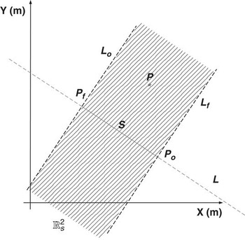
A segment's region is defined as follows. Let S be a segment associated with line L and Po and Pf be its endpoints in the considered region. Let Lo and Lf be two lines normal to L that pass through Po and Pf, respectively. A point P belongs to a region of S if it belongs to the area delimited by Lo and Lf that contains S. Figure 11 shows a representation of the region of a segment.
Region of a segment. A navigable point is influenced by the probability distribution associated with a line if that point belongs to the region of the segment of the line

Thus, those points that belong to the region of a segment are probabilistically influenced by the line that contains that segment in the SLAM system state.
By considering that a line is represented in polar coordinates by a point in the polar plane, any other point represented in the polar space will imply line at the Cartesian space. According to this, to calculate the probability of a point with respect to a line is necessary to determine to which line the point belongs. Considering that a line feature has a Gaussian distribution function, its maximum probability value occurs on their mean values. Thus, those values that make null the kernel of the Gaussian distribution represent the points where the probability reaches its maximum. In this work, it was adopted that the line to which the point of the environment belongs is a parallel of the line feature of the map. Thus, the angle between them will be null in the kernel of the Gaussian distribution and only the distance will be computed. Equation (14) shows the probability of a point with respect to a line when the point belongs to a parallel of the line feature.
 $$P{{({{p}_{x,y}})}_{line,k}}\: = \:\frac{1}{{\sqrt {{{{(2\pi )}}^2} \:|\:{{{\rm{\rPsi }}}_k}|} }}{{e}^{{\rm{ - }}\frac{1}{2}{{{(\rUpsilon {\rm{ - }}\rGamma )}}^T} {\rm{\rPsi }}_{k}^{{{\rm{ - }}1}} (\rUpsilon {\rm{ - }}\rGamma )}} $$
In Equation (14),  $\rPsi$k is the covariance of the line extracted from the covariance matrix of the SLAM system state,
 $ {{\rUpsilon }^T} \: = \:{{[\sigma \,\tau ]}^T} $ are the parameters of the line extracted from the SLAM system state. If the line were virtual, for example, the lines that contain the edges of the circumscribing rectangle in Section 4.1—then
 $ {{\rUpsilon }_{virtual}} $ contains the parameters that define the line and its covariance could be of the form
 $ {{\rPsi }_{virtual}}\: = \:\left[ \matrix { {0.32} & {0.0} \cr\ {0.0} & {0.32} \\\end{}} \right] $. Note that
 $\rPsi$virtual is not unique.
 $ {{\rGamma }^T} \: = \:{{[{{\sigma }_p} {{\tau }_p}]}^T} $ represents the parameters of the parallel line that contains the navigable point px ,y. As stated before, σp = σ in Equation (14) because the lines are parallel.
4.1.5 Weighted sum of Gaussians method
To calculate the probability of a navigational point within the environment, it is necessary to calculate how all the mapped features are influencing it. Thus, considering that all features mapped from the environment have a Gaussian distribution function, in this work the weighted sum of Gaussians method was used in order to infer the probability associated with a navigable point. The weighted sum of Gaussians method is faster when compared with other fusion methods (Sanchez Miralles & Sanz Bobi, Reference Sanchez Miralles and Sanz Bobi2004) and could be applied for both: real and virtual features. The resulting probability is always smaller than one. Let L be the number of features contained in  $ {{\hat{\xi }}_{m,t}} $, the part of the SLAM system state composed of the extracted features from the environment—see Equation (1). Also, let Lc and Ll the number of mapped corners and lines, respectively, such that L = Lc + Ll. Furthermore, let Ll ,v be the number of virtual lines. The virtual lines correspond to the segments that circumscribe the environment. Equation (15) shows the sum of Gaussians implementation having into account both: real and virtual features.
 $$ \matrix {{ & P({{p}_{x,y}})\: = \:} \cr\ { & \mathop{\sum}\limits_{k\: = \:1}^{{{L}_c}} \frac{{{{{\epsilon}}_{c,k}}{{\sigma }_{c,k}}}}{{\sqrt {{{{(2\pi )}}^2} |{{\rPsi }_{c,k}}|} }}{{e}^{{\rm{ - }}\frac{1}{2}{{{\left( {\left[ \matrix { {{{p}_x}} \cr\ {{{p}_y}} \\\end{}} \right]{\rm{ - }}\left[ \matrix { {{{\sigma }_{c,k}}\cos ({{\tau }_{c,k}})} \cr\ {{{\sigma }_{c,k}}\sin ({{\tau }_{c,k}})} \\\end{}} \right]} \right)}}^T} \rPsi _{{c,k}}^{{{\rm{ - }}1}} \left( {\left[ \matrix { {{{p}_x}} \cr\ {{{p}_y}} \\\end{}} \right]{\rm{ - }}\left[ \matrix { {{{\sigma }_{c,k}}\cos ({{\tau }_{c,k}})} \cr\ {{{\sigma }_{c,k}}\sin ({{\tau }_{c,k}})} \\\end{}} \right]} \right)}} } \cr { & + {\mathop{\sum}\limits_{k\: = \:1}^{{{L}_l}} \frac{{{{{\epsilon}}_{l,k}}}}{{\sqrt {{{{(2\pi )}}^2} |{{\rPsi }_{l,k}}|} }}{{e}^{{\rm{ - }}\frac{1}{2}{{{\left( {{{\rUpsilon }_{l,k}}{\rm{ - }}{{\rGamma }_{l,k}}} \right)}}^T} \rPsi _{{l,k}}^{{{\rm{ - }}1}} \left( {{{\rUpsilon }_{l,k}}{\rm{ - }}{{\rGamma }_{l,k}}} \right)}} }} \cr\ { & + \mathop{\sum}\limits_{k\: = \:\,1}^{{{L}_{l,v}}} \frac{{{{{\epsilon}}_{l,v,k}}}}{{\sqrt {{{{(2\pi )}}^2} |{{\rPsi }_{l,v,k}}|} }}{{e}^{{\rm{ - }}\frac{1}{2}{{{\left( {{{\Upsilon }_{l,v,k}}{\rm{ - }}{{\rGamma }_{l,v,k}}} \right)}}^T} \rPsi _{{l,v,k}}^{{{\rm{ - }}1}} \left( {{{\rUpsilon }_{l,v,k}}{\rm{ - }}{{\rGamma }_{l,v,k}}} \right)}} } \\\end{}$$
In Equation (15),  $\rPsi$c,k,
 $\rPsi$l,k and
 $\rPsi$l,v,k are the covariance matrices associated with the kth corner, line and virtual line, respectively; εc ,k, εl ,k and εl,v ,k are the weights associated with each term of the sum of Gaussians method such that the result, P(px,y), is always smaller than one. The weight factors in Equation (15) were obtained according to Sanchez Miralles and Sanz Bobi (Reference Sanchez Miralles and Sanz Bobi2004). The mechanism shown in Sections 4.1.3–4.1.5 allows the estimation of an occupational probability value of each navigable point of the map obtained in Section 4.1.2.
4.1.6 Monte Carlo uncertainty maps examples
Figure 12 shows three examples of the construction of uncertainty maps based on the procedure presented above. Figure 12(a) and (d) are partial reconstructions of the facilities of the Instituto de Automatica of the National University of San Juan, and Figure 12(g) is an office environment of the Engineering Department of the Federal University of Espirito Santo, Brazil. Figure 12(a), (d) and (g) show the reconstruction of the map based on the SLAM system state and covariance matrix. The solid black segments correspond to walls associated with lines; light grey circles are corners and the dotted grey line is path traveled by the mobile robot. The grey points are raw data acquired by the range sensor laser incorporated on the robot.
Examples of the construction of uncertainty maps. Figure 12(a), (d) and (g) shows three different environment reconstructions using the extended Kalman filter—Simultaneous Localization and Mapping (EKF—SLAM) algorithm presented in this work; Figure 12(b), (e) and (h) show the Monte Carlo points generation after circumscribing the map obtained by the EKF–SLAM by the virtual rectangle—solid black segments. Figure 12(b), (e) and (h) correspond to Figure 12(a), (d) and (g), respectively. Figure 12(c), (f) and (i) show the uncertainty maps after applying the sum of Gaussians method to each Monte Carlo point of Figure 12(b), (e) and (h)

Figure 12(a), (e) and (h) show the mapped environment—solid black lines—circumscribed by the virtual rectangle—solid red lines. The small grey squares represent the Monte Carlo points generated within the circumscribed area. The light grey circles are corners of the environment. The number of generated Monte Carlo points for the three figures was of M = 1000.
In addition, Figure 12(c), (f) and (i) show the uncertainty maps after applying the sum of Gaussians method to each Monte Carlo point. Although in Section 4.1.5 it was stated that the probability value is calculated over the set of navigational points of the environment, in order to see the entire probability map, the probability value in Figure 12(b), (e) and (h) was calculated for all the Monte Carlo points. As it can be seen, the light grey areas in such figures represent the uncertainty areas that will be used as navigation goals (if the uncertainty point associated with them is a navigational point). In this work, an uncertainty point was considered as such if its probability value was P(px ,y) = 0.5 ± 0.2. Thus, the navigational points whose probability value laid in the range of 0.5 ± 0.2 were considered as uncertainty points, because no conclusions can be made about their occupational status.
4.2 Autonomous Simultaneous Localization and Mapping navigation
As stated in Section 4.1, a navigable point will be considered as an uncertainty point if the probability value associated with it remains in a neighborhood of 0.5.
Once an uncertainty point is found, a trajectory is planned from the robot's pose to that point, using the information of the environment provided by the SLAM system state. Then, a trajectory follower controller drives the robot to a neighborhood of the uncertainty point goal. Considering that we are using range sensors to map the environment, the fact of reaching the actual position of the uncertainty point is not needed, because the robot is able to map the environment surrounding that point by means of the range sensor. During the navigation, the SLAM algorithm is continuously executed. The trajectory controller implemented in this work is the Kanayama's controller (Kanayama et al., Reference Kanayama, Kimura, Miyazaki and Noguchi1990).
If more than one uncertainty point is found, then a selection criterion is used to determine which point will be the goal of the navigation. Equation (16) shows the goal selection criterion, where dist(.) represents the distance between two points and P(px,y) is the probability associated with point px,y according to Equation (15). Thus, for n uncertainty points, only the one that has the maximum ratio between its probability value and its distance from the robot will be chosen as a navigation goal. Further information can be found in a previous work of the authors (Auat Cheein et al., Reference Auat Cheein, Toibero, Lobo Pereira, di Sciascio and Carelli2010); kj is a priority value associated with the uncertainty point, as will be explained below:
 $$Goal\ Navigation\ Uncertainty\ Point\: = \:\frac{1}{{{{\kappa }_j}}} max\left\{ {\frac{{P({{p}_{x,y{{|}_i}}})}}{{dist(robo{{t}_{pose}},{{p}_{x,y{{|}_i}}})}}} \right\};\; \; i\: = \:1 \ldots n$$
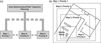
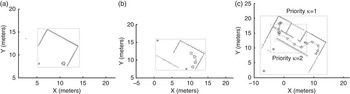
Considering that the size of the map increases during the navigation, the uncertainty point determination is made in several levels with different priorities associated with each level. Figure 13 shows the multilevel uncertainty points searching. Each level is implemented in a different thread, therefore, all levels work in parallel. For example, for the map shown in Figure 13(b), the main map is divided into k levels. Each level has a virtual rectangle circumscribing it. All the virtual rectangles have the same orientation with respect to the main map. The priority assignment is as follows: the main map has the higher priority—priority κ = 1—and the k-level has priority κ = k, where k is an integer. Thus, when the navigation system is looking for a goal, the uncertainty points within all the different levels are searched. An uncertainty point with priority 1, for example, is chosen when compared with an uncertainty point of priority 3. The uncertainty points searching of level k−1 does not include the virtual features of level k, it only works with the real features of the environment and its own virtual circumscribing rectangle. The navigation strategy based on the multilevel uncertainty point searching is shown in the following section.
Parallel implementation of the multilevel uncertainty point searching. (a) Shows the parallel structure of the implementation and (b) shows the multilevel division: each level has a priority associated with it

4.2.1 Mobile robot navigation strategy
The navigation strategy can be summarized as follows:
1. Let us suppose that the robot's initial pose is
$ {{[{{\hat{\xi }}_x}\ {{\hat{\xi }}_y}\ {{\hat{\xi }}_\theta }]}^T} \: = \:{{[{{\hat{\xi }}_{x,0}}\ {{\hat{\xi }}_{y,0}}\ {{\hat{\xi }}_{\theta, 0}}]}^T} $ referenced to a global reference frame previously established during the initial conditions declaration of the SLAM algorithm. The mobile robot performs, without moving, the first features extraction procedure of the navigation.2. A first circumscribing rectangle is determined. This rectangle must circumscribe all extracted features from the environment and the robot's pose. If no features were detected, then a generic size circumscribing rectangle including the robot's pose can be used instead.
3. M Monte Carlo points are uniformly generated within the circumscribing rectangle. Then, from the M Monte Carlo points, only the
$ N\: \subseteq \:M $ navigable points are used.4. A probability value is associated with each navigable point. In order to do this, the sum of Gaussians method is used. The sum of Gaussians method has into account the probability of the point with respect to any feature—real or virtual—of the environment. A real feature is a feature that is modeled by the SLAM system state and its covariance matrix. As stated before, the edges of the circumscribing rectangle will be considered as Gaussian virtual features with probability value of 0.5 associated with its parameters.
5. A navigable point will be considered as an uncertainty point if its probability value is in a neighborhood of 0.5. From the set of
$ L\: \subseteq \:N\: \subseteq \:M $ uncertainty points, only one will be chosen as navigation goal according to Equation (16).6. Once an uncertainty point is found, a trajectory is planned from the robot's current pose to the uncertainty point. Then, the Kanayama's trajectory controller drives the robot to a neighborhood of that point.
7. When the robot reaches a neighborhood of the uncertainty point, a new uncertainty point should be determined from the information within the SLAM system state and its covariance matrix by means of the procedure mentioned above.
8. If any edge of the virtual rectangle that circumscribes the mapped area is bigger than the range of the sensor used, then the map is organized in several nested levels as it is shown in Figure 13(b). Up to eight different levels are allowed in our work. All the levels are equally placed from the robot's pose to the main map.
9. The system searches for uncertainty points within all the levels as it is shown in Figure 13. Considering that, at the same time, not all levels will find an uncertainty point goal, the navigation strategy chooses a low priority level uncertainty point according to Equation (16), until a high priority level uncertainty point is found.
10. Once a high priority level uncertainty point is found, a trajectory is planned from the robot's current pose to the uncertainty point and the trajectory controller drives the robot motion to it.
11. Once the robot reaches an uncertainty point, the searching strategy is repeated only in those levels that are not currently working.
12. If after a finite number of attempts and despite of the path planned, the robot is not able to reach the navigation goal, then that goal is replaced by a new uncertainty point destination.


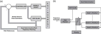
The navigation strategy presented above can also be interpreted as follows: the mobile robot remains navigating based on local uncertainty points until global uncertainty points are found, then the robot is driven to them. Figure 14 shows the final SLAM-Control architecture implemented in this work. As Figure 14(a) shows, the SLAM algorithm provides the robot's pose references to the controller and the map information to the trajectory planner. Figure 14(b) shows how the priorities of each level of uncertainty maps are managed by the navigation system; the multiplexer, according to the priority level, chooses between the different uncertainty maps.
Simultaneous Localization and Mapping (SLAM)-Control architecture. (a) The SLAM algorithm closes the loop providing the robot's pose information to the controller and the environment information to the trajectory planner and (b) the different levels of the uncertainty maps are combined by a multiplexer governed by the priority values of each navigation goals

4.2.2 Non-reactive controllers: trajectory follower controller
The non-reactive controller implemented in this work is the Kanayama's trajectory controller for non-holonomic vehicles (Kanayama et al., Reference Kanayama, Kimura, Miyazaki and Noguchi1990). This is an asymptotically stable control law whose stability was proved through Lyapunov theory. The inputs to the vehicle controller are the reference posture [xr yr θr]T and the reference velocities [Vr Wr]T.
The posture error is defined as follows:
 $$\left[ \matrix { {{{x}_e}} \cr\ {{{y}_e}} \cr\ {{{\theta }_e}} \\\end{}} \right]\: = \:\left[ \matrix { {\cos ({{{\hat{\xi }}}_{\theta, t}})} & {\sin ({{{\hat{\xi }}}_{\theta, t}})} & 0 \cr\ {{\rm{ - }}\sin ({{{\hat{\xi }}}_{\theta, t}})} & {\cos ({{{\hat{\xi }}}_{\theta, t}})} & 0 \cr\ 0 & 0 & 1 \\\end{}} \right]\left[ \matrix { {{{x}_r}{\rm{ - }}{{{\hat{\xi }}}_{x,t}}} \cr\ {{{y}_r}{\rm{ - }}{{{\hat{\xi }}}_{y,t}}} \cr\ {{{\theta }_r}{\rm{ - }}{{{\hat{\xi }}}_{\theta, t}}} \\\end{}} \right]$$
where  $ {{[{{\hat{\xi }}_{x,t}}\,{{\hat{\xi }}_{y,t}}\,{{\hat{\xi }}_{\theta, t}}]}^T} $ is the current estimated pose of the vehicle.
The control law is
 $$\left[ \matrix { V \cr\ W \\\end{}} \right]\: = \:\left[ \matrix { {{{V}_r}\cos {{\theta }_e}\: + \:{{K}_x}{{x}_e}} \cr\ {{{W}_r}\: + \:{{V}_r}({{K}_y}{{y}_e}\: + \:{{K}_\theta }\sin {{\theta }_e})} \\\end{}} \right]$$
where Kx, Ky and Kθ are positive constants.
Kanayama also proposes a parameter selection to obtain a critical damping in the control. The damping of the tracking control can be calculated through
 $$ \zeta \: = \:\frac{{{{K}_\theta }}}{{2\sqrt {{{K}_y}} }} $$
A critical damping in the control is obtained when ζ = 1.
The path associated with the trajectory was previously obtained by implementing the non-optimum path planning method presented by Nieto et al. (Reference Nieto, Slawinski, Mut and Wagner2010). Then, with the references positions of the path and the estimated pose of the vehicle by the SLAM system state, the trajectory follower was implemented according to Equation (18).
5 Experimental results
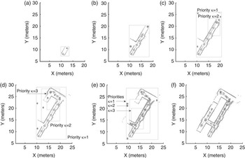
Several real-time experiments of the SLAM-Control proposal presented in Section 4.2 are shown in this section. The maximum SLAM sampling time was of 0.2 s. The last implies that the pause, the features extraction and the SLAM execution in Figure 5(b) were performed within a maximum time of 0.2 s during the navigation of the mobile robot. In addition, the features association criterion used in this work corresponds to the Mahalanobis distance (Guivant & Nebot, Reference Guivant and Nebot2001; Thrun et al., Reference Thrun, Burgard and Fox2005). Figure 15 shows results of the SLAM-based map reconstruction for a simulated office environment, whereas Figure 16 shows different snapshots of the experiments carried out at the facilities of the Instituto de Automatica of the National University of San Juan.
Real-time simulation of the navigation strategy. This figure shows the map reconstruction and the navigation of the mobile robot within a simulated office environment. The solid grey lines are the rectangles that circumscribe the environment; the light grey points are raw laser data; the dark grey lines are segments associated with lines and light grey circles represent corners; and the solid grey dots represent the center of mass of a cloud of uncertainty points over that region. (a) Shows the first execution of the Simultaneous Localization and Mapping (SLAM) algorithm while the robot remains still; (b) shows the second execution of the SLAM and (c) after several executions and given the size of the mapped area, the uncertainty points procedure requires two levels of searching

Real-time experimentation of the navigation strategy within a real environment. The light grey lines represent the edges of the circumscribing rectangle; solid dark grey lines are walls associated with lines of the environment; dotted black line is the path traveled by the mobile robot; light grey circles are corners and solid grey circles are the center of mass of a cloud of uncertainty points over that region; and grey dots are raw laser data. Figure 16(a)–(f) show different snapshots of the evolution of the mobile robot navigation within the facilities of the Instituto de Automatica of the National University of San Juan. (a) The first features from the environment are acquired and added to the SLAM system state while the mobile robot remains still; (b) shows another searching of uncertainty points using a single level map; (c) given the dimensions of the current map, the uncertainty points are searched within two levels; (d) and (e) the system requires three priority levels of uncertainty points searching; and (f) shows the complete map of the environment

The mobile robot used was the non-holonomic unicycle type Pioneer 3AT (built by ActivMedia) with a range sensor laser (built by SICK) incorporated on it. The laser acquires 181 range measurements between 0° and 180°. The measurement range was set to 7 m, although the laser can be set up to 32 m. No odometry information was used in the SLAM algorithm.
For the uncertainty maps construction, the maximum number of Monte Carlo points for the level with the smallest priority (which is the closest level to the local reference frame of the mobile robot) was of M = 1000—although M is adjustable. The maximum number of levels of uncertainty points searching paralleled implemented in this work was of eight levels. The number of Monte Carlo points for each level was a linear function of the priority associated with the corresponding level of the uncertainty map. Thus, for an uncertainty map with priority k = 8, M = 1000—as stated before—and for an uncertainty map with priority κ = 1, M = 8 × 1000 = 8000 points. In Figures 15 and 16, the uncertainty points—that could be used as possible destination goals—are represented by solid red circles. These solid red circles represent the center of mass of a cloud of uncertainty points located in the corresponding region.
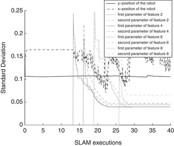
In addition, Figure 17 shows the behavior of the standard deviation associated with the position of the mobile robot and with the parameters of several features during the SLAM-Control executions shown in the real-time experiment of Figure 16. As it can be seen, the standard deviation remains bounded during the estimation of the SLAM system state.
Standard deviation evolution of the robot's position and feature's parameters during the Simultaneous Localization and Mapping (SLAM) algorithm executions of the experiment shown in Figure 16. The standard deviation remains bounded

6 Conclusions
This paper has presented the advantages and methods of introducing a predictor to compensate the no-constant time executions of a sequential EKF–SLAM when implemented with a non-reactive controller, such as a path or a trajectory follower. The EKF–SLAM algorithm used in this work was a feature-based SLAM that extracts corners and lines from the environment. In order to show real-time implementations of the combination of the SLAM algorithm with non-reactive controllers, an uncertainty maps construction based on the Monte Carlo method was shown. The construction of uncertainty maps has allowed the determination of unvisited regions—called uncertainty points—of the environment. A trajectory controller has driven the vehicle from its current pose to the uncertainty points.
The Monte Carlo method to build uncertainty maps has introduced a new method to generate a probabilistic map of the environment considering all features as Gaussian distributions without the need of gridding the map. The method uses the Gaussianity condition of the features of the environment acquired during the SLAM algorithm execution.
The navigation strategy presented in this work has searched for uncertainty points within different levels of the mapped environment. Each level had an uncertainty map with a priority associated with it. Levels closer to the local reference frame of the mobile robot had a priority smaller than the levels closer to the global reference frame of the vehicle. Once an uncertainty point was found, the trajectory controller had driven the robot to a neighborhood of that point. During the navigation and the construction process, the SLAM algorithm was continuously executed.
Experimental results about the probabilistic map construction were also shown. The entire system was implemented in real time showing its autonomy and performance when mapping and navigating unknown environments. The SLAM algorithm and the navigation strategy were implemented to build a geometric map of the environment, although they were restricted to structured ones. For future works, the SLAM algorithm and the navigation strategy will be implemented to operate in open and semi-structured environments.
Acknowledgment
The authors would like to thank CONICET-Argentina and FCT-Portugal for partially founding this research.