


1. INTRODUCTION
Consider the following prediction problem. We have independent and identically distributed random pairs (X,Y),(X1,Y1),…,(Xn,Yn) from

, where the label space

is a subset of

. The aim is to use the data (X1,Y1),…,(Xn,Yn) to choose a function

with small risk, R(fn) = E[ell ](Y,fn(X)), where [ell ] is a nonnegative loss function. Ideally, the risk should be close to the minimal or Bayes risk, R* = inff R( f ), where the infimum is over all measurable functions. A natural approach is to minimize the empirical risk,

, over some class

of functions. Clearly, there is a trade-off in the choice of

: we can decompose the excess risk of fn as

where the first term represents the estimation error and the second the approximation error. We would like both terms in the decomposition to be small. For the first term to be small,

should be sufficiently small that it is possible to use the data to choose a near-optimal function from

based on the data. For the second term to be small,

should be sufficiently large that it contains a good approximation to the optimal prediction.
One approach to this problem is to choose a large class

and decompose it into

then choose

to minimize the empirical risk, and finally choose the model index j so that

best balances these conflicting requirements. In this paper, we consider complexity penalization approaches, in which we choose

with

chosen to minimize a combination of the empirical risk of

and a penalty term:

where the penalty pj depends on the sample size n.
We are interested in oracle inequalities of the form

where c is a positive constant. In such an inequality, if the term cpj decreases with n at the same rate as the estimation error

, then the inequality shows that our choice fn has excess risk that decreases at the same rate as if we had the advice of an oracle who tells us the best complexity class

to choose. The utility of an oracle inequality of this kind depends on the accuracy with which the penalty term approximates the estimation error.
It is well known that such inequalities follow easily from uniform convergence results, as illustrated by the following theorem. The proof is immediate (see, e.g., Bartlett, Boucheron, and Lugosi, 2002).
THEOREM 1. If the data are such that

then in that case

Notice that the first inequality of the theorem involves random variables. Thus, when it holds with high probability, the second inequality of the theorem holds with high probability.
The theorem shows that it suffices to choose the penalty pj as a high-probability upper bound on the maximal deviation between empirical risks and risks. But it is sometimes possible to obtain faster rates of convergence (smaller values of pj as a function of n) than could be implied by the uniform convergence results. Indeed, the following theorem shows that for a nontrivial function class and loss function, the maximal deviation between

and R(f) can approach zero at a rate no faster than n−1/2 (see, e.g., Bartlett and Mendelson, 2006, Thm. 2.3).
THEOREM 2. There is a constant c such that, for any loss function

and any function class

for which

, we have

On the other hand, for the quadratic loss

or the exponential loss

used by the pattern classification method AdaBoost (Freund and Schapire, 1997), for example, and for

a convex bounded subset of a finite-dimensional linear class, the empirical minimizer

can approach

at the faster rate of O(n−1 log n), as the following theorem shows. (The theorem is an easy consequence of Theorem 3.3 in Bartlett, Bousquet, and Mendelson, 2005, Lemmas 14 and 15 in Bartlett, Jordan, and McAuliffe, 2006, and an application of the entropy integral of Dudley, 1999—see, e.g., the proof of Corollary 3.7 in Bartlett et al., 2005.)
THEOREM 3. Suppose [ell ] : [0,1]2 → [0,1] satisfies the Lipschitz condition

and the uniform convexity condition

Then there is a constant c for which the following condition holds. Suppose that

is convex and a subset of a d-dimensional linear space. Let the distribution of the random pairs (X,Y),(X1,Y1),…,(Xn,Yn) be such that the minimizer

exists. Then for all x > 0, with probability at least 1 − e−x,


Clearly, for the empirical minimizer

, the term

in the first inequality of the theorem is nonpositive, and so with probability at least 1 − e−x,

Results of this kind were first shown for the quadratic loss and function classes with small covering numbers (Lee, Bartlett, and Williamson, 1996) and later generalized to strictly convex normed spaces and classes with small covering numbers (Mendelson, 2002) and strictly convex losses and classes with small local Rademacher averages (Bartlett et al., 2005, 2006); see also Koltchinskii (2006). There are many examples for which these bounds on estimation error decrease at essentially the best possible rate (see, e.g., Massart, 2000).
Although these results show that the risk of the empirical minimizer converges to the minimal risk in the function class surprisingly quickly, it is not clear that the results are useful for complexity penalization. Is it possible to perform model selection by choosing the class with the smallest penalized empirical risk, and will this lead to an oracle inequality with the corresponding fast rate? It has been suggested that this is not possible: see, for example, the comments in Section 2.1 of Blanchard, Lugosi, and Vayatis (2003). Indeed, Theorem 2 shows that, although the empirical minimizer's risk approaches the minimal risk roughly as n−1 in the example of Theorem 3, we cannot hope to estimate the minimal risk (or the risk of any function in the class with nonconstant loss) to better accuracy than n−1/2.
In this paper, we give a simple proof that, for nested hierarchies, the fast rates in inequalities of the kind that appear in Theorem 3 do imply oracle inequalities for complexity penalization methods. Thus, although the empirical risks that are used to compare classes in the hierarchy fluctuate on a scale that can be large compared to the complexity penalties, for nested hierarchies the fluctuations are sufficiently correlated that they do not excessively affect our choice of class.
2. ORACLE INEQUALITIES
As before, consider the following complexity penalization approach. Decompose a class

of real-valued functions defined on an input space

into a sequence of subsets

,

,…. For each j, define the empirical risk minimizer and the true risk minimizer in the class

as


Assign to each class

a complexity penalty pj. Then choose

, where

THEOREM 4. Suppose that the classes are ordered by inclusion, choose positive numbers εk that are similarly ordered,


and choose a penalty pk = 7εk/2. Then if the data are such that


this implies that

Notice as before that the inequalities (1) and (2) involve random variables. Thus, when they hold with high probability (such as under the conditions of Theorem 3), then the final inequality of the theorem holds with high probability.
If we apply (1) to the empirical minimizer

in a single class

, the difference

is nonpositive, and so we obtain

The theorem shows that adding an O(εk) penalty to the empirical risks allows us to choose the class k that satisfies the best of these inequalities. The intuition behind condition (1) is that for functions with small regret (i.e., the difference between their risk and the minimal risk over the class is small), the empirical regret should be a more accurate upper bound on the regret, whereas it need not be so accurate for functions with large regret. Condition (2) provides corresponding lower bounds. This second condition is necessary to ensure that the penalized estimate does not choose the class

too large.
3. PROOF
We set pj = cεj for some constant c, and we shall see later that c = 7/2 suffices.
First we show that

will have risk that is not much worse than that of any

from a larger class,

.
LEMMA 5. In the event that

,

Proof. From the condition (1), we see that for any j,

In addition, the definition of

implies

Thus, we have

because

. Applying (1) for the class

, we have
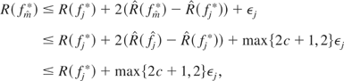
by definition of

. Thus, applying (1) again, this time for the class

, we have

The next step is to show that the risk of

cannot be much worse than that of any

from a smaller class

. First, we show that the risk of the optimal function from

is not much bigger than the risk of the optimal function from any smaller class.
LEMMA 6. In the event that

,

Although it is immediate that

in this case, we shall see that we need to ensure that, for a suitably large penalty, the gap decreases with

. This is where the condition (2) is important: it allows us to show that

is not chosen too large.
Proof. We have

The result follows. █
Next we show that this implies that the risk of

is not much larger than the risk of any

from a smaller class.
LEMMA 7. In the event that

,

Proof. From (1) and the previous lemma,

Choosing c = 7/2 gives the result. █


