



1. Introduction
Scalar turbulence refers to the chaotic transport and mixing of passive scalar quantities, such as temperature, chemical concentration or pollutant levels, within turbulent flows (Shraiman & Siggia Reference Sirivat and Warhaft2000). This phenomenon holds profound significance across numerous scientific and engineering disciplines (Dimotakis Reference Dimotakis2005). A comprehensive understanding of how scalars evolve under turbulent conditions is essential for predictive modelling and practical control in applications, ranging from pollutant dispersion in atmospheric and oceanic flows, to combustion optimisation in engines and efficient mixing in chemical processing. In contrast to velocity turbulence, which addresses the chaotic behaviour of velocity fluctuations, scalar turbulence examines the interplay between turbulent advection, where scalar fields are stretched and folded by the flow, and molecular diffusion, which smooths scalar gradients at small scales. Together, these mechanisms govern the mixing, dissipation and ultimate influence of scalars on system behaviour (Sreenivasan Reference Talluru, Philip and Chauhan2019).
Given by the ‘passive’ nature, the passive scalar dynamics are believed to be determined by the velocity turbulence, and are often taken as the dynamics mirrored from the velocity characteristics. In terms of the velocity turbulence, an essential characteristic is how the turbulent energy cascades from large scale down to small scales, which are usually quantified by the velocity spectra or structure functions of velocity fluctuations. The Kolmogorov milestone theoretical framework predicts a scaling over the wavenumbers far away from both the forcing and the viscous scales. Equivalently, the second-order structure function exhibits the power scaling among separation length scales. For the turbulence in shear flow with a mean convection speed, in addition to the energy cascade of the velocity fluctuations, the characteristic speed of the convection with which the fluctuations of physical quantities co-move is additionally essential to quantify the turbulence. Space–time correlations of the velocity fluctuations
 $R_{uu}$
can quantify the characteristic convection speeds, in addition to characterising the cascade (taking its Fourier transformation relation with the spectra) (He & Tong Reference He and Xu2011; He et al. Reference He and Zhang2017). For instance,
 $R_{uu}(\delta ,\tau )=\langle u'(z+\delta ,t+\tau )\,u'(z,t) \rangle /[u_{\textit{rms}}(z)u_{\textit{rms}}(z+\delta )]$
, where
 $u'$
is the fluctuation of streamwise velocity
 $u$
;
 $\delta$
and
 $\tau$
are space and time separation, respectively,
 $\langle {\cdot }\rangle$
is an ensemble averaging operation, and
 $u_{\textit{rms}}$
is the root mean square (RMS) of the corresponding velocity. Kim & Hussain (Reference Kim and Hussain1993) implemented the space–time correlation to extract the characteristic convection speed, which at the channel wall is approximately
 $0.5U_c$
, with
 $U_c$
the time-averaged velocity
 $\langle U \rangle$
at the channel centre, significantly differing from the time-averaged velocity at the wall,
 $\langle U \rangle =0$
. Later studies confirm such differences in the canonical channel flows (Jiménez et al. Reference Jiménez, del Álamo and Flores2004; Flores & Jiménez Reference Flores and Jiménez2006; Geng et al. Reference Geng, He, Wang, Xu, Lozano-Durán and Wallace2015) with a new method (del Álamo & Jiménez Reference Corrsin2009) exploring the convection speed among wavenumbers, emphasising the necessity of investigating the convection speed via the space–time correlations.
Similarly, the scalar convection speed
 $U_\phi$
represents the speed at which these scalar structures are advected by the flow (Kim & Hussain Reference Kim and Hussain1993). Although frequently approximated as the mean flow velocity,
 $U_\phi$
may diverge from this value in flows influenced by dispersion or the growth and decay of disturbances (Kim & Moin Reference Kim and Moin1989; Kim & Hussain Reference Kim and Hussain1993). Previous studies of passive scalar turbulence on the space–time correlations mostly consider the Schmidt numbers
 $\textit{Sc} = \nu /\kappa$
near unity (e.g.
 $\textit{Sc} \approx 0.8$
in air flows, and
 $\textit{Sc} \approx 5$
in liquid flows), where
 $\nu$
is kinematic viscosity, and
 $\kappa$
is the molecular diffusivity. These investigations (e.g. He & Tong Reference He and Xu2011; Zhou et al. Reference Zimmerman, Antonia, Djenidi, Philip and Klewicki2011; Hogg & Ahlers Reference Hogg and Ahlers2013) were mainly conducted in turbulent Rayleigh–Bénard convection, where temperature is formally an active scalar. However, in the bulk region away from the boundary layers, buoyancy effects are relatively weak, and temperature fluctuations behave approximately as a passive scalar, under which scalar space–time correlations were reported to exhibit similarities to velocity correlations. This is consistent with other quantities between the passive scalar and the velocity fields (e.g. Kim & Moin Reference Kim and Moin1989; Abe & Antonia Reference Abe and Antonia2009; Antonia et al. Reference del Álamo and Jiménez2009). However, the small-scale dynamics of scalar mixing are believed to be influenced by the Schmidt number and are potentially different (Sreenivasan Reference Talluru, Philip and Chauhan2019; Pirozzoli Reference Pirozzoli, Bernardini and Orlandi2023) when the Schmidt number is away from unity, such as in liquid metal convection (
 $\textit{Sc} \sim 10^{-2}$
) (Zwirner et al. Reference Zwirner, Khalilov, Kolesnichenko, Mamykin, Mandrykin, Pavlinov, Shestakov, Teimurazov, Frick and Shishkina2020) and water–ethanol mixing (
 $\textit{Sc} \sim 10^{3}$
) (Schikarski et al. Reference Schumacher and Sreenivasan2017; Sreenivasan Reference Talluru, Philip and Chauhan2019). Specifically, spectral studies (e.g. Yeh & Atta Reference Yeung and Pope1973; Warhaft & Lumley Reference Willis1978; Jayesh & Warhaft Reference Jayesh and Warhaft1994; Warhaft Reference Warhaft and Lumley2000; Gylfason & Warhaft Reference Gylfason and Warhaft2004; Iyer et al. Reference Iyer, Schumacher, Sreenivasan and Yeung2018) have demonstrated that the scalar energy spectrum generally exhibits a broader inertial scaling range than the velocity field at comparable Taylor-scale Reynolds number (
 $\textit{Re}_\lambda$
). In addition, recent studies have demonstrated that the second-order structure function of the scalar increment displays a dependence on
 $\textit{Sc}$
(e.g. Buaria et al. Reference Buaria, Clay, Sreenivasan and Yeung2016, Reference Brethouwer, Boersma, Pourquié and Nieuwstadt2021a
,
Reference Buaria, Clay, Sreenivasan and Yeungb
). While these studies have significantly advanced our understanding of scale-by-scale statistics in space, the corresponding space–time correlation characteristics of passive scalar fluctuations remain far less explored. In terms of characterising space–time correlations (He & Tong Reference He and Xu2011; He et al. Reference He and Zhang2017), in addition to the scalar convection speed, the scalar Taylor microscale
 $\lambda _\phi$
is an important quantity (Warhaft & Lumley Reference Willis1978; George Reference George1992). Analogous to the Taylor microscale in velocity field
 $\lambda _u$
(Taylor Reference Tennekes and Lumley1935), the scalar Taylor microscale, an intermediate length scale associated with scalar gradient and scalar dissipation rate (Corrsin Reference Comte-Bellot and Corrsin1951; Monin et al. Reference Nguyen and Papavassiliou1979; George Reference George1992; Fox Reference Fox2003), quantifies dynamically significant scalar structures, offering insight into the fine-scale mixing processes that are often challenging to resolve experimentally (Comte-Bellot & Corrsin Reference Clay, Buaria, Gotoh and Yeung1966; Sirivat & Warhaft Reference Song, Barkley, Hof and Avila1983; Wang & George Reference Warhaft2002). The effect of the Schmidt number on the scalar Taylor microscale is also not well understood. It is not easy to well control the Schmidt numbers spanning a wide range in practice to explore the convection speed and the Taylor microscale, given that available passive scalar (i.e. dyes) mixing in liquid has similar Schmidt numbers
 $\mathcal{O}(10^3)$
, and temperature in air has
 $\mathcal{O}(1)$
. Another important issue is that many previous studies considered statistically stationary scalar turbulence, such as homogeneous turbulence maintained by a mean scalar gradient (e.g. Gotoh & Watanabe Reference Gotoh and Watanabe2015; Buaria et al. Reference Brethouwer, Boersma, Pourquié and Nieuwstadt2021a
) or wall-bounded scalar fields under imposed wall or bulk scalar boundary conditions (e.g. Kawamura et al. Reference Kawamura, Abe and Matsuo1999; Abe et al. Reference Abe, Kawamura and Matsuo2004; Pirozzoli et al. Reference Pope2022). In contrast, many practical scalar mixing problems are transient and involve spatially developing, in which scalar structures evolve downstream and retain memory of their release. In such flows, the scalar convection velocity and scalar Taylor microscale may depend not only on molecular diffusivity, but also on the local downstream mixing state. This space–time aspect of Schmidt-number-dependent scalar transport has received comparatively less attention.
In this study, we examine the space–time correlations of the scalar fluctuations in a fully developed pipe flow with a localised scalar plume at Reynolds number
 $\textit{Re} = 10\,000$
, particularly investigating how molecular diffusivity affects scalar transport across regimes from
 $\textit{Sc} = 10^{-3}$
to
 $\textit{Sc} = 10$
. This configuration differs from statistically homogeneous scalar turbulence maintained by a uniform mean scalar gradient or from wall-bounded scalar fields under imposed wall or bulk scalar boundary conditions. To accomplish this, we employ a hybrid computational approach integrating direct numerical simulations (DNS) for the velocity field with Lagrangian scalar tracking (LST) (Kontomaris et al. Reference Kraichnan1992; Papavassiliou & Hanratty Reference Pirozzoli1997; Nguyen & Papavassiliou Reference Oksendal2018) for the scalar field. The DNS resolve the full scales of turbulent velocity field, while the LST tracks the evolution of passive scalar markers, accounting for both convective transport and diffusive spreading. Based on the same set of velocity fields, the dynamics of scalar fields from diverse Schmidt numbers can be isolated and examined. By analysing space–time correlations of the scalar fluctuations, we obtain the scalar convection speed and the scalar Taylor microscale, and examine their corresponding dependence on the Schmidt number, shedding light on how molecular diffusion mediates the dynamics of scalar fields. The computational method is introduced in § 2. The results and discussions are in §§ 3 and 4, respectively. The conclusions are drawn in § 5.
2. Computational method
2.1. Simulation of flow velocity field
The velocity field is simulated using DNS for an incompressible, Newtonian fluid with constant density and viscosity in a fully developed pipe flow. The governing equations are the incompressible Navier–Stokes equations
 \begin{equation} \frac {\partial \boldsymbol{u}}{\partial t}+\boldsymbol{u} \boldsymbol{\cdot }\boldsymbol{\nabla } \boldsymbol{u}=-\boldsymbol{\nabla }\!p+\frac {1}{\textit{Re}} {\nabla} ^2 \boldsymbol{u}, \quad \boldsymbol{\nabla } \boldsymbol{\cdot }\boldsymbol{u}=0, \end{equation}
where
 $\boldsymbol{u}$
is the velocity,
 $p$
is the pressure, and
 $\textit{Re} = 10\,000$
is the Reynolds number defined based on the pipe diameter
 $D$
and bulk velocity
 $U$
. The flow is driven by a constant volume flux, maintaining a fixed bulk speed throughout the simulation. The equations are solved in cylindrical coordinates
 $(r,\theta ,z)$
using a spectral finite-difference method. An open-source pipe flow code Openpipeflow (Willis & Kerswell Reference Wu and He2009; Willis Reference Willis and Kerswell2017) is used to perform the simulations. No-slip boundary conditions are applied at the pipe wall
 $(u(r/D=0.5,\theta ,z,t) = 0)$
, with periodicity enforced in the axial (
 $z$
) and azimuthal (
 $\theta$
) directions. The computational domain extends
 $6.25D$
in length. In the periodic directions, 576 and 432 Fourier modes are employed for the axial and azimuthal discretisations, respectively. In the radial direction, a finite-difference scheme with a 9-point stencil is used, discretised over 128 grid points, clustered near the pipe wall, to resolve the boundary layer accurately (see Willis (Reference Willis and Kerswell2017) for details). Time integration proceeds with step size
 $2.5 \times 10^{-4}$
in advection time (
 $D/U$
). Once the turbulence reaches a statistically stationary state, instantaneous flow fields are saved every
 $1 \times 10^{-3} (D/U)$
, defining the sampling interval
 $T_s$
. Since
 $T_s$
determines the largest resolved frequency, it should satisfy
 $T_s \leqslant \eta _B/U$
in order to resolve the energy-containing convection line, where
 $\eta _B$
is the Batchelor scale, given by
 $\eta _B=\eta _K\, \textit{Sc}^{-1/2}$
for
 $\textit{Sc} \gt 1$
(Batchelor Reference Bahri, Arwatz, George, Mueller and Hultmark1959; Kraichnan Reference Lavertu and Mydlarski1968), with
 $\eta _K \approx 0.0069D$
at the pipe centre (Cerbus et al. Reference Buaria, Yeung and Sawford2020; Zimmerman et al. Reference Zwirner, Khalilov, Kolesnichenko, Mamykin, Mandrykin, Pavlinov, Shestakov, Teimurazov, Frick and Shishkina2022). Here,
 $\eta _K$
is the Kolmogorov length scale at the pipe centreline. Note that for
 $\textit{Sc} \leqslant 1$
,
 $T_s \leqslant \eta _K/U$
are satisfied because the mixing is not completed at Obukhov–Corrsin scale until approximately the Kolmogorov scale (Sawford Reference Sawford and Sullivan2006; Eyink Reference Eyink2011).
Comparison of velocity field from the present simulation (
 $\textit{Re} = 10\,000$
) with El Khoury et al. (Reference El Khoury, Schlatter, Noorani, Fischer, Brethouwer and Johansson2013) at
 $\textit{Re} = 11700$
. (a) Profiles of mean axial velocity (
 $U_z^+$
):
 $U_z^+ = y^+$
and
 $U_z^+ = k^{-1} \ln y^+ + B$
with
 $k = 0.41$
and
 $B = 5.2$
are given as grey dashed lines. (b) Axial turbulent intensity (
 $\langle u_z^2 \rangle$
). (c) Radial turbulent intensity (
 $\langle u_r^2 \rangle$
). (d) Reynolds shear stress (
 $\langle u_zu_r \rangle$
) in inner scaling as a function of
 $y^+$
.

The inner-scaled velocity statistics from the present DNS at
 $\textit{Re}=10\,000$
are compared in figure 1 with the reference DNS data of El Khoury et al. (Reference El Khoury, Schlatter, Noorani, Fischer, Brethouwer and Johansson2013) at a slightly higher Reynolds number (
 $\textit{Re}=11\,700$
). As shown in figure 1(a), the mean axial velocity profile agrees well with the reference data across the viscous sublayer, buffer layer and logarithmic region, and closely follows both the linear law (
 $U_z^+=y^+$
) and the logarithmic law. Small deviations appear in the outer part of the logarithmic region, which are likely attributable to the difference in Reynolds number. The Reynolds normal stresses shown in figures 1(b) and 1(c) exhibit similar trends in the two datasets. In particular, the peak locations are well reproduced, although the present results slightly underpredict the peak magnitudes relative to the reference data. A similarly good agreement is observed for the Reynolds shear stress in figure 1(d), where the near-wall behaviour and the peak position are both captured well, with only minor discrepancies in the outer region. Overall, the close agreement between the two datasets indicates that the present simulation reliably captures the main features of turbulent pipe flow despite the moderate Reynolds number difference. Furthermore, Openpipeflow employed in this study has been extensively validated and widely used in previous investigations of turbulent pipe flow (e.g. Willis & Kerswell Reference Wu and He2009; Avila et al. Reference Armenio, Piomelli and Fiorotto2010; Song et al. Reference Sreenivasan2017; Willis Reference Willis and Kerswell2017; Yao et al. Reference Yeh and Atta2023), which further supports the accuracy and robustness of the present simulations.
2.2. The LST approach
Passive scalar markers, representing massless particles, are introduced into the flow to simulate scalar transport without influencing the flow dynamics. Their trajectories are computed by numerically integrating the stochastic differential equation
 \begin{equation} \text{d} \boldsymbol{x}(t)= \boldsymbol{u} (\boldsymbol{x}({t}), t) \ \text{d} t+\sqrt {2 \kappa } \ \text{d} \boldsymbol{W}_{\!{t}}, \end{equation}
where
 $\boldsymbol{x}$
is the marker position,
 $\boldsymbol{u}(\boldsymbol{x}(t), t)$
is the fluid velocity at that position,
 $\kappa$
is the molecular diffusivity, and
 $\boldsymbol{W}_{\!{t}}$
is a Wiener process modelling Gaussian white noise (Eyink Reference Eyink2011; He & Xu Reference He, He and Tong2025). This equation captures both convective motion (via the velocity term) and diffusive motion (via the stochastic term). In this equation, the motion of scalar markers was decomposed into a convection part and a molecular diffusion part. The convective part can be calculated from the fluid velocity at the particle position, so that the Lagrangian velocity at time
 $t$
of a marker released at location
 $\boldsymbol{x}$
, at time zero, is assumed to be the same as the Eulerian velocity at that particle’s location. The effect of molecular diffusion follows from Einstein’s theory for Brownian motion, in which the rate of molecular diffusion is related to the molecular diffusivity
 $\kappa$
. The diffusion effect is simulated by adding a random movement on the particle motion at the end of each convective step. In numerical simulation, equation (2.2) is integrated using the Euler–Maruyama scheme
 \begin{equation} \boldsymbol{x}_{n+1}(t+\Delta t)=\boldsymbol{x}_n(t) + \boldsymbol{u}(\boldsymbol{x}_n(t))\, \Delta t + \sqrt {2 \kappa }\, \Delta \boldsymbol{W}_{\!{n}}(\Delta t), \end{equation}
where
 $\Delta t$
is the integration time step, and
 $\Delta \boldsymbol{W}_{\!{n}}$
denotes the increments of a Wiener process, which follow a Gaussian distribution
 $\mathcal{N}$
, i.e.
 $\Delta \boldsymbol{W}_{\!{n}} \sim \mathcal{N}(\mu = 0, \sigma ^2 = \Delta t)$
(e.g. Sawford Reference Sawford2001; Eyink Reference Eyink2011; He & Xu Reference He, He and Tong2025). In the present implementation, the marker integration time step is chosen to be equal to the sampling interval of the stored DNS velocity fields, i.e.
 $\Delta t=T_s$
. The value of
 $T_s$
is chosen such that the marker displacement associated with both turbulent advection and molecular diffusion during one time step remains within the range where the DNS velocity field is assumed to be spatially smooth (e.g. Eyink Reference Eyink2011; He & Xu Reference He, He and Tong2025). In practice, for
 $\textit{Sc}\gt 1$
, we require
 $T_s \leqslant \eta _B/U$
, while for
 $\textit{Sc}\leqslant 1$
, we require
 $T_s \leqslant \eta _K/U$
as a conservative condition. These advective displacement constraints are more restrictive than the corresponding diffusive time scale constraints, which equal Kolmogorov time
 $\tau _K$
when
 $\textit{Sc} \geqslant 1$
, and
 $\tau _K\, {Sc}^{-1/2}$
when
 $\textit{Sc}\lt 1$
(He & Xu Reference He, He and Tong2025). The scalar velocity
 $\boldsymbol{u}(\boldsymbol{x}_n(t))$
is interpolated by a cubic spline method (Yeung & Pope Reference Yeung and Sreenivasan1988; Kontomaris et al. Reference Kontomaris, Hanratty and McLaughlin1992) between the Eulerian velocity field values from DNS (see § 2.1) at the surrounding mesh points. Given that the storage of DNS velocity fields with time interval smaller than the Kolmogorov time scale and the corresponding velocity field is approximately linear for the spatial scales smaller than the Kolmogorov scale, the interpolation method has trivial influence from example tests (not shown) on the correlation statistics in this study. This approach has also been applied in Kontomaris et al. (Reference Kraichnan1992), Papavassiliou & Hanratty (Reference Pirozzoli1997), Sawford (Reference Sawford and Sullivan2006), Eyink (Reference Eyink2011) and Nguyen & Papavassiliou (Reference Oksendal2018). At the pipe wall, an impermeable boundary condition is imposed for the scalar markers. To prevent stochastic displacements from possibly moving markers out through the boundary of the computational domain, a marker is frozen there when it is too close to the wall (i.e.
 $y^+\lt 1$
), following the strategy of Armenio et al. (Reference Antonia, Abe and Kawamura1999). We have checked our simulation that only a very small fraction of markers,
 $\mathcal{O}(10^{-6})$
, enter this near-wall region, therefore this treatment is expected to have trivial influence on the reported scalar statistics (statistics closest to wall are taken at
 $y^+\approx 5$
). The markers’ velocities and positions are recorded at each time step for statistical analysis.
2.3. Seeding scalar markers and Eulerian scalar concentration
Parameter setting in the LST simulations.

Table 1. Long description
A table comparing parameter settings in LST simulations. The table has four columns and six rows. The columns are labeled Re, Sc, Number of scalar markers, and Tracers generated every 0.005 (D/U). The rows present different values for these parameters. Row 1: Re, 10 000; Sc, 10^-3; Number of scalar markers, 5 x 10^8; Tracers generated every 0.005 (D/U), 1 x 10^6. Row 2: Re, 10 000; Sc, 10^-2; Number of scalar markers, 5 x 10^8; Tracers generated every 0.005 (D/U), 1 x 10^6. Row 3: Re, 10 000; Sc, 10^-1; Number of scalar markers, 5 x 10^8; Tracers generated every 0.005 (D/U), 1 x 10^6. Row 4: Re, 10 000; Sc, 1; Number of scalar markers, 5 x 10^8; Tracers generated every 0.005 (D/U), 1 x 10^6. Row 5: Re, 10 000; Sc, 5; Number of scalar markers, 10 x 10^8; Tracers generated every 0.005 (D/U), 2 x 10^6. Row 6: Re, 10 000; Sc, 10; Number of scalar markers, 20 x 10^8; Tracers generated every 0.005 (D/U), 4 x 10^6.
(a) Sketch of the initial scalar marker release from five localised concentric annular sources at
 $r/D=0.05$
,
 $0.15$
,
 $0.25$
,
 $0.35$
and
 $0.45$
. The dark bands illustrate the random generation of scalar markers on one annular source. (b) Probability density functions (PDFs) of the radial positions of released scalar markers for each annular source, showing the narrow Gaussian distribution around each prescribed radius. (c) Sketch of the time series of the tracer generation, where the circle symbols mean the tracer generation (the symbols are skipped for clarity). (d) Sketch of the rendering plane (including the coordinates), marked by the grey dashed lines.

Snapshots of the scalar field at
 $\textit{Re} = 10\,000$
for (a)
 $\textit{Sc} = 10^{-3}$
, (b)
 $\textit{Sc} = 1$
and (c)
 $\textit{Sc} = 10$
at the same time instant. The first row denotes the three-dimensional scalar concentration structures rendered by the iso-concentration
 $\phi =0.12$
and the arrows showing the flow direction; the second and third rows denote the corresponding radial-azimuthal and streamwise-radial cross-sections of the scalar concentration (see the right-hand colour map), respectively. (d) The scalar profiles for
 $\textit{Sc} = 10^{-3}$
, 1 and 10. The inset shows the zoomed region for
 $z/D = 3.1{-}3.3$
. (e) The mean profiles of the scalar field for
 $3\leqslant z/D\leqslant 4$
, which are normalised by their own peaks of Gaussian fitting. The lines are the Gaussian fitting results, and the symbols are the simulation results.

The scalar field is constructed by tracking the positions of scalar markers over time, combining DNS and LST methodologies. Initially, scalar markers are released concurrently from five localised concentric annular sources located at
 $r/D=0.05$
,
 $0.15$
,
 $0.25$
,
 $0.35$
and
 $0.45$
. For each source, the radial positions of the released markers follow a Gaussian distribution centred at the prescribed radius, with standard deviation
 $0.015D$
, while their azimuthal positions are randomly distributed along the annulus, as shown in figures 2(a) and 2(b). The same number of markers are released from each annular source. The fixed amount of scalar markers is generated every
 $0.005D/U$
(see table 1), and ceases after time
 $2.5D/U$
(see figure 2
c), allowing the markers to disperse and mix within the flow. In order to obtain enough markers for statistics, several independent simulation runs are performed under identical flow and scalar conditions. The total number of scalar markers reported in table 1 corresponds to the cumulative number obtained by combining all runs. To visualise the scalar field, the pipe volume is divided into planes with bins. For each given
 $r{-}z$
plane, the thickness is also
 $\eta _B$
for
 $\textit{Sc} \gt 1$
(
 $\eta _{K}$
for
 $\textit{Sc} \leqslant 1$
). This process mimics the planar laser induced fluorescence (PLIF) process. Bin sizes are set to
 $\varDelta _r = \varDelta _z = \eta _B$
for
 $\textit{Sc} \gt 1$
(
 $\eta _{K}$
for
 $\textit{Sc} \leqslant 1$
), ensuring resolution of the smallest scalar structures. Note that for
 $\textit{Sc} \leqslant 1$
, the Obukhov–Corrsin scale is not used, because the mixing is not completed until the Kolmogorov scale. The numbers of bins in the radial and axial directions are
 \begin{equation} N_r = \frac {D}{2\varDelta _r},\quad N_z = \frac {6.25D}{\varDelta _z}. \end{equation}
Each bin, denoted as
 $N(i,j)$
for
 $1 \leqslant i \leqslant N_r$
and
 $1 \leqslant j \leqslant N_z$
, records the number of markers within it. The scalar concentration
 $\phi$
is approximated as
 $N(i,j)/(2^8-1)$
, simulating an 8-bit output of an image sensor. Snapshots at the same moment of the concentration field for various Schmidt numbers are presented in figures 3(a–c). Given by the discontinuous release of the tracer markers (releasing once every other four time steps), pearl-necklace-like filament structures can be observed, and this is more evident for larger Schmidt numbers, given that the scalar markers diffuse more slowly at larger Schmidt numbers. As shown in figures 3(a–c), it can be observed that large scalar structures are visually similar for different
 $\textit{Sc}$
, but internal striations of finer scale accompany larger
 $\textit{Sc}$
, especially
 $\textit{Sc}=10$
in figure 3(c). Similar effects of Schmidt numbers on scalar flow structures are also observed in a homogeneously sheared flow (Schumacher & Sreenivasan Reference Shete, Boucher, Riley and de Bruyn Kops2003). The mean scalar profiles at
 $z/D=3.5$
(taken as a representative downstream location) are shown in figure 3(e). These profiles are well approximated by the fitted Gaussian curves (lines), and their widths increase slightly with increasing
 $\textit{Sc}$
. Similar Gaussian-like scalar profiles in turbulent pipe flow, channel flow, grid turbulence and turbulent boundary layer flow with point or line releasing of scalar have also been reported by Brethouwer et al. (Reference Boppana, Xie and Castro1999), Boppana et al. (Reference Batchelor2012), Bahri et al. (Reference Avila, Willis and Hof2015) and Talluru et al. (Reference Talluru, Philip and Chauhan2018). These studies attribute the emergence of such profiles to the possible dominance of isotropic turbulent diffusion during the early stage of downstream convection. It is also worth noting that the classic logarithmic mean scalar profile (e.g. Kader’s law; Kader Reference Kader1981) typically emerges in statistically stationary wall-bounded flows under constant wall heat flux or constant bulk temperature boundary conditions, as observed in DNS studies such as Kawamura et al. (Reference Kawamura, Abe and Matsuo1999), Abe et al. (Reference Abe, Kawamura and Matsuo2004) and Pirozzoli et al. (Reference Pirozzoli, Romero, Fatica, Verzicco and Orlandi2016, Reference Pope2022). In those cases, the scalar field adjusts to a quasi-equilibrium state with the turbulent boundary layer. In contrast, the present simulation considers a transient mixing process originating from a localised concentric source, without imposed wall heat flux or bulk temperature constraints. Although the velocity field is statistically stationary, the scalar field evolves from an initially compact plume and therefore remains far from the equilibrium conditions considered in Kawamura et al. (Reference Kawamura, Abe and Matsuo1999), Abe et al. (Reference Abe, Kawamura and Matsuo2004) and Pirozzoli et al. (Reference Pirozzoli, Romero, Fatica, Verzicco and Orlandi2016, Reference Pope2022). In the present simulations, the mean scalar profiles show negligible variation over short streamwise distance approximately
 $1D$
. Consequently, the region
 $3 \leqslant z/D \leqslant 4$
is used for subsequent analysis. Within this limited streamwise range, a local statistical steady state is assumed, meaning that the scalar statistics at a fixed downstream location are statistically stationary in time under continuous scalar release. Because of the discontinuous release and the finite number of markers, some large mixing structures seem to be broken at small scales in the rendered images, unlike the PLIF measurements where there are countless fluorescent molecules and infinite light rays. Finite number of rendered snapshots necessitates a convergence study, which was carried out in § A.2 to examine and ensure statistical reliability of the correlation
 $R_{\phi \phi }$
.
3. Results
3.1. Space–time correlation of scalar fluctuations
The two-point space–time correlation
 $R_{\phi \phi }(\delta /D, \tau U/D)$
represents the statistical relationship between scalar field values separated by a spatial separation
 $z$
and a time separation
 $\tau$
. It is defined as
 \begin{equation} R_{\phi \phi }(\delta /D, \tau U/D) = \frac {\langle \phi ^\prime (z+\delta /D, t+\tau U/D)\, \phi ^\prime (z, t)\rangle }{\phi _{\textit{rms}}(z)\, \phi _{\textit{rms}}(z+\delta /D)}, \end{equation}
where
 $\phi ^\prime (z)$
is a scalar concentration fluctuation at spatial position
 $z$
, and
 $\phi _{\textit{rms}}$
denotes the RMS of
 $\phi$
. Here,
 $\phi ^\prime = \phi - \langle \phi \rangle$
, with
 $\langle \phi \rangle$
the time-averaged scalar concentration. In addition,
 $\delta$
and
 $\tau$
are the space separation along the streamwise direction and time separation, respectively, and
 $\left \langle {\cdot }\right \rangle$
denotes the ensemble averaging operation. The distance separation
 $\delta$
is taken along the streamwise direction
 $z$
at a radial position. Examples of the space–time correlations are taken at
 $r/D=0.3$
within a streamwise range
 $3\leqslant z/D \leqslant 4$
. Contours of the correlation
 $R_{\phi \phi }$
for Schmidt numbers
 $\textit{Sc} = 10^{-3}$
,
 $1$
and
 $10$
are shown in figures 4(b–d). In addition, the space–time correlation of velocity fluctuations
 $R_{uu}(\tau ,\delta )$
is shown in contours of figure 4(a) for comparison. In this figure, the iso-correlation lines of
 $R_{uu}$
exhibit elliptical shapes, agreeing with the elliptical approximation framework of He et al. (Reference He and Zhang2017). Similar observations are also evidenced in experiments of turbulent pipe flows (Li et al. Reference Mohaghar, Dasi and Webster2025) and turbulent channel flows (Kim & Moin Reference Kim and Moin1989; He & Zhang Reference He and Tong2006). Regarding the scalar correlation
 $R_{\phi \phi }$
, for
 $\textit{Sc}=10^{-3}$
, the iso-correlation lines also display clear elliptical shapes. For
 $\textit{Sc}=1$
, the elliptical iso-correlation curves turn out to be narrower, and they are further narrower for
 $\textit{Sc}=10$
. As the time separation
 $\tau$
increases, the
 $R_{uu}$
curves have smaller peaks, and the widths of the curves are roughly unchanged. Similar observations can be found in
 $R_{\phi \phi }$
for each of the Schmidt numbers. Among the different Schmidt numbers,
 $R_{\phi \phi }$
curves are narrower as
 $\textit{Sc}$
increases. This implies that as the Schmidt number increases, the scalar fluctuations decorrelate more rapidly. As the Schmidt number increases, the scalar diffuses to the surroundings more slowly; the concentration conserved structures are not correlated in space and time. If the Schmidt number is assumed to approach infinity, then the scalar concentration field is assumed to be uncorrelated, as considered in the Kraichnan model (Kraichnan Reference Lavertu and Mydlarski1968; Falkovich et al. Reference Falkovich, Gawȩdzki and Vergassola2001; Yang et al. Reference Yao, Rezaeiravesh, Schlatter and Hussain2023).
(a) Space–time correlation of velocity fluctuations
 $R_{uu}(\tau ,\delta )$
. (b–d) Space–time correlations
 $R_{\phi \phi }(\tau ,\delta )$
for (b)
 $\textit{Sc} = 10^{-3}$
, (c)
 $\textit{Sc} = 1$
and (d)
 $\textit{Sc} = 10$
. The black lines denote lines of iso-correlation (a)
 $R_{\phi \phi }=0.96$
and
 $0.98$
, (b–d)
 $R_{\phi \phi }=0.5$
and
 $0.6$
. All correlations are obtained at
 $r/D = 0.3$
and
 $3\leqslant z/D\leqslant 4$
.

The correlation contours differ from the one in the Rayleigh–Bérnard convection (He & Zhang Reference He and Tong2006; Zhou et al. Reference Zimmerman, Antonia, Djenidi, Philip and Klewicki2011), where the contours display circular-like shapes in the centre of the convection cell given by the lack of mean advection, and elliptical shapes from the large-scale flow motion near the cell wall.
3.2. Convection velocity of scalar fluctuations
The measured peak position
 $\delta _p/D$
as a function of
 $\tau U/D$
for the scalar and velocity field, corresponding to figure 4.

Scalar convection speed at the streamwise
 $z/D = 3.5$
. (a) Radial profiles of the scalar convection speed
 $U_\phi /U_c$
at different Schmidt numbers
 $\textit{Sc}$
, where
 $U_c=\langle U(r=0) \rangle$
. (b) The scalar convection speed in wall unit
 $U^+_\phi$
along the distance from the pipe wall in wall unit
 $y^+$
. (c) The scalar convection speed normalised by the local mean velocity. (d) The contour of the ratio
 ${U}_\phi /{U}_u$
. (e) The ratio of the mean scalar convection speed
 $\overline {U}_\phi$
and the mean convection speed of velocity fluctuations
 $\overline {U}_u$
as a function of
 $\textit{Sc}$
.

The convection speed of the scalar field,
 $U_\phi$
, can be determined by analysing the space–time correlation of the scalar field, following established methods (Kim & Hussain Reference Kim and Hussain1993; He et al. Reference He, Jin and Yang2010; Zhou et al. Reference Zimmerman, Antonia, Djenidi, Philip and Klewicki2011; Hogg & Ahlers Reference Hogg and Ahlers2013). Specifically,
 $U_\phi$
is calculated from a position (
 $\delta _p$
) that maximises
 $R_{\phi \phi }$
for a given time separation (
 $\tau U/D$
), i.e.
 $\delta _p=\mathrm{max}(R_{\phi \phi }\,|\,\tau )$
. As shown in figure 5, the peak positions
 $\delta _p$
exhibit an approximately linear dependence on the time separation
 $\tau$
for all Schmidt numbers. The convection velocity
 $U_\phi$
is obtained from a linear fit to the relation
 $\delta _p = U_\phi \tau$
over the range
 $0 \leqslant \tau U/D \leqslant 0.08$
, where the linear behaviour is clearly observed. The same fitting range is consistently applied to all
 $\textit{Sc}$
cases and radial positions to ensure comparability. A similar linear trend is also observed for the velocity correlation
 $R_{uu}$
, consistent with previous studies (He et al. Reference He, Jin and Yang2010; Zhou et al. Reference Zimmerman, Antonia, Djenidi, Philip and Klewicki2011; Hogg & Ahlers Reference Hogg and Ahlers2013).
This process is repeated for each pipe radial position, giving the profiles of the convection speed shown in figure 6(a), while the corresponding ratio of the convection speed with the local mean velocity is shown in figure 6(c). The convection speed profile of the velocity fluctuations in the pipe flow is similar to that in the turbulent channel flow (Kim & Hussain Reference Kim and Hussain1993; Jiménez et al. Reference Jiménez, del Álamo and Flores2004; Flores & Jiménez Reference Flores and Jiménez2006; del Álamo & Jiménez Reference Corrsin2009; Geng et al. Reference Geng, He, Wang, Xu, Lozano-Durán and Wallace2015). For instance, close to the wall, the convection speed is approximately
 $0.55$
, or
 $U^+_\phi \approx 11.5$
for the distance from the wall
 $y^+\lt 10$
(see figures 6
a,b), although the Schmidt numbers are different among the studies. For the scalar mixing, at
 $\textit{Sc}=1$
, the
 $U_\phi$
profile nearly collapses with the velocity convection profile, which is also similar to
 $\langle U \rangle$
for
 $r/D \lesssim 0.48$
. When
 $\textit{Sc}\lt 1$
, e.g.
 $\textit{Sc}=10^{-3}$
, high molecular diffusivity increases the spreading of scalar structures, reducing their coherence and effective propagation speed, thus lowering
 $U_\phi$
. Conversely, for
 $\textit{Sc} \gt 1$
, reduced diffusivity preserves compact scalar structures, with their convection enhanced by the turbulent flow. These results challenge the assumption that
 $U_\phi$
equals the mean flow velocity, especially in flows with
 $\textit{Sc} \neq 1$
. Close to the wall, the scalar convection speed ranges from
 $U_\phi /U_c\approx 0.5$
to
 $U_\phi /U_c\approx 0.56$
for
 $\textit{Sc}$
from
 $10^{-3}$
to
 $10$
, and in wall units
 $11\lesssim U_\phi ^+ \lesssim 12$
for
 $10^{-3} \leqslant Sc \leqslant 10$
. This finding has implications that experimental data relying on Taylor’s frozen turbulence hypothesis needs close examination (Zaman & Hussain Reference Zhou, Li, Lu and Liu1981; Geng et al. Reference Geng, He, Wang, Xu, Lozano-Durán and Wallace2015), and suggests that
 $\textit{Sc}$
-dependent corrections may be required to accurately transform temporal data into spatial information, especially for the turbulence close to the wall.
To further examine the spatial dependence of the Schmidt number effect, figure 6(d) shows the contours of the ratio
 $U_\phi /U_u$
as a function of the radial position (
 $r/D$
) and
 $\textit{Sc}$
. It can be seen that the influence of
 $\textit{Sc}$
on the scalar convection speed extends over a broad region of the pipe cross-section. Although the magnitude of
 $U_\phi /U_u$
varies with
 $r/D$
, particularly near the wall, the overall trend of increasing
 $U_\phi$
relative to
 $U_u$
with the increase of
 $\textit{Sc}$
remains consistent across most radial locations. A shallow local minimum can be observed near
 $r/D \approx 0.45$
for
 $\textit{Sc}=10^{-3}$
to
 $1$
, indicating a slight reduction of
 $U_\phi /U_u$
in the outer region at low Schmidt numbers. For higher Schmidt numbers (
 $\textit{Sc}=5$
and
 $10$
), a mild bulge of
 $U_\phi /U_u$
appears in the region
 $r/D \approx 0.2{-}0.45$
, suggesting enhanced scalar convection relative to velocity fluctuations in this intermediate radial range. With the
 $U_\phi$
profile, the cross-sectional average of the scalar convection speed is obtained as
 \begin{equation} \overline {U}_\phi = \frac {\int _{0}^{D/2} 2 \pi U_\phi r\, \mathrm{d} r}{\int _{0}^{D/2} 2 \pi r\, \mathrm{d} r}=(8/D^2)\int _{0}^{D/2} U_\phi r\, \mathrm{d} r. \end{equation}
Similarly, with the
 $U_u$
profile, the mean velocity convection speed (
 $\overline {U}_u$
) can be obtained. The effect of the Schmidt number on the mean convection speed is summarised in figure 6(e). For
 $\textit{Sc}\lesssim 1$
,
 $\overline {U}_\phi$
increases mildly with
 $\textit{Sc}$
, approaching
 $\overline {U}_u$
at
 $\textit{Sc}\approx 1$
. As
 $\textit{Sc}$
further increases,
 $\overline {U}_\phi$
continues to increase, indicating that scalar fluctuations are convected slightly faster than velocity fluctuations. However, the dependence on
 $\textit{Sc}$
remains relatively weak over the present range, and is therefore interpreted as a qualitative trend rather than a well-defined scaling law. If the observed trend is assumed to persist, then as
 $\textit{Sc}$
approaches zero,
 $U_\phi$
approaches zero. In this asymptotic limit, the scalar concentration is extremely rapidly uniform in space, and correspondingly
 $R_{\phi \phi }$
tends to unity for any space and/or time separations. However,
 $U_\phi$
approaching zero seems to be physically infeasible, speculated from the observation that the smallest advection speed of the velocity field is not zero although the ensemble-averaged velocity is zero there. As
 $\textit{Sc} \rightarrow \infty$
, if the scaling persists, then
 $U_\phi$
approaches infinity, and this is physically infeasible; in such a circumstance,
 $R_{\phi \phi }$
would tends to be a delta function for any small space or time separation, and
 $U_\phi$
cannot be extracted from such a correlation. Based on these discussions, we cautiously conjecture that
 $U_\phi (Sc)$
with
 $\textit{Sc}$
may approach an upper-bound saturation. A hypothetical upper bound is
 ${U}_u(r=0)$
, corresponding to the maximum convection speed of velocity fluctuations in a wall-bounded turbulent flow from a statistical perspective. The scalar convection speed, inferred from scalar space–time correlations, should therefore be interpreted as a statistical signal velocity associated with the underlying turbulent velocity field. At high
 $\textit{Sc}$
, molecular diffusion is very weak, and thin scalar filaments can persist over longer times. These filaments are not transported as rigid frozen objects, but are continuously stretched, tilted and deformed by the turbulent velocity field while being slowly smoothed by molecular diffusion. Thus the measured
 $U_\phi$
indicates the combined effects of turbulent advection and filament deformation. As a result, the measured
 $U_\phi$
may become more strongly associated with relatively fast-moving turbulent motions. In this sense,
 ${U}_u(r=0)$
may serve as a plausible statistical reference for the upper limiting behaviour of
 $U_\phi$
.
Similarly, as
 $\textit{Sc}$
decreases towards zero, stronger molecular diffusion suppresses thin scalar filaments, and produces broader, smoother scalar structures. The scalar field then loses small-scale spatial coherence more rapidly, and the scalar convection speed may approach the velocity convection speed and even a lower-bound saturation conjecturally close to
 ${U}_u(r/D=0.5)$
, which corresponds to the minimum convection velocity of velocity fluctuations in the present flow. This interpretation is consistent with the fact that passive scalar transport is mediated by the velocity field through the advection–diffusion equation, while its apparent propagation also depends on diffusion and structural deformation. We emphasise that this interpretation should be regarded only as a tentative hypothesis based on the trends observed within the limited Schmidt number range considered here, rather than as a complete physical argument or a rigorously established asymptotic result. Since the present dataset is not sufficient to confirm the proposed saturation behaviour, further work is needed to verify this trend over a broader range of Schmidt numbers, and to investigate the detailed physical mechanisms responsible for it. A more conclusive assessment would require additional data, especially at more extreme
 $\textit{Sc}$
, together with velocity–scalar space–time correlation analysis, conditional structural analysis and further theoretical investigation.
Scale-dependent convection velocity of scalar fluctuations at the streamwise
 $z/D = 3.5$
. Wavenumber-dependent scalar convection velocity
 $U_k^\phi$
as a function of streamwise wavenumber
 $k_z D$
at different radial locations, compared with the velocity-field convection velocity
 $U_k^u$
(symbols), for (a)
 $\textit{Sc} = 10^{-3}$
, (b)
 $\textit{Sc} = 1$
and (c)
 $\textit{Sc} = 10$
. Different line styles denote different radial positions. (d–f) Contours of the ratio
 $U_k^\phi /U_k^u$
as a function of Schmidt number
 $\textit{Sc}$
and wavenumber
 $k_z D$
at
 $r/D = 0$
,
 $0.2$
and
 $0.4$
, respectively. The results show that the
 $\textit{Sc}$
dependence of the convection velocity is strongly scale-dependent, with enhanced convection velocity at high
 $\textit{Sc}$
primarily associated with small-scale (high-wavenumber) scalar structures.

The dependence of the scalar convection velocity on
 $\textit{Sc}$
suggests that the relevant transport mechanism is scale selective. To quantify this effect, we analyse the convection velocity as a function of wavenumber using the space–time spectrum. Following del Álamo & Jiménez (Reference Corrsin2009) and Wu & He (Reference Wu and He2021a
,
Reference Yang, Pan and Heb
), the convection velocity associated with a given wavenumber is obtained from the space–time spectrum
 $E(k,f)$
, namely
 \begin{equation} U_k(k) = \frac {f_c(k)}{k}, \quad f_c(k) = \frac {\int f E(k,f)\,\mathrm{d}f}{E(k)}. \end{equation}
Applying this definition to the scalar spectrum (
 $E_\phi$
) and velocity spectrum (
 $E_u$
) gives the scale-dependent convection velocities
 $U_k^\phi$
and
 $U_k^u$
, respectively. In this framework, the convection velocity shown in figure 6(a) is recovered as a spectrum-weighted average, namely,
 $U = {\int U_k(k)\,k^2\,E(k)\,\mathrm{d}k}/{\int k^2\,E(k)\,\mathrm{d}k}$
. Figures 7(a–c) show the variation of
 $U_k^\phi$
with the streamwise wavenumber
 $k_z D$
at different radial locations. It is observed that the scalar convection velocity depends weakly on wavenumber at low
 $\textit{Sc}$
, while a clear scale dependence emerges as
 $\textit{Sc}$
increases. In particular, for
 $\textit{Sc}\gt 1$
,
 $U_k^\phi$
exceeds
 $U_k^u$
over a broad range of intermediate and high wavenumbers, indicating that small-scale scalar structures are convected faster than the corresponding velocity fluctuations. The scale-dependent behaviour is more clearly illustrated in figures 7(d–f), which show the ratio
 $U_k^\phi /U_k^u$
as a function of
 $\textit{Sc}$
and
 $k_z D$
. For increasing
 $\textit{Sc}$
, the enhancement of convection velocity is primarily concentrated at high wavenumbers, whereas large-scale motions remain comparatively less affected. This demonstrates that the
 $\textit{Sc}$
-dependence of the convection velocity is intrinsically linked to the spectral distribution of scalar fluctuations. Physically, at high Schmidt numbers, molecular diffusion is weak, allowing scalar fluctuations to persist at small scales (e.g. Buaria et al. Reference Brethouwer, Boersma, Pourquié and Nieuwstadt2021a
,
Reference Buaria, Clay, Sreenivasan and Yeungb
). These scalar structures may be statistically associated with relatively fast-moving turbulent motions, and thus impose a higher effective convection velocity. In contrast, at low
 $\textit{Sc}$
, diffusion suppresses small-scale scalar structures, leading to a dominance of larger, smoother scalar features that exhibit lower convection velocities. This scale-dependent interpretation provides an association to the observed
 $\textit{Sc}$
-dependent convection velocity, and agrees with the interpretation that the scalar transport characteristics are governed by the interplay between scalar diffusivity and the multiscale structure of turbulence. The present analysis does not directly identify the instantaneous velocity structures responsible for scalar transport; further investigation using velocity–scalar space–time cross-correlations or conditional structural analysis would be needed.
The space–time correlation profiles
 $R_{uu}(\tau U/D=0)$
and
 $R_{\phi \phi }(\tau U/D=0)$
at
 $r/D=0.3$
at the streamwise
 $z/D = 3.5$
.

3.3. Taylor microscale
Another important quantity from the space–time correlation is the Taylor microscale. In turbulence, the Taylor microscale of velocity fluctuations, introduced by Taylor (Reference Tennekes and Lumley1935), characterises an intermediate length scale in turbulent flows that marks the transition from the inertial range, where viscosity has minimal impact, to the dissipation range, where viscous forces dominate and kinetic energy is converted to heat (Tennekes & Lumley Reference Villermaux1972; Pope Reference Sawford2000). Specifically, in the context of a scalar field, the scalar Taylor microscale
 $\lambda _\phi$
represents the intermediate scale where molecular diffusion begins to influence turbulent scalar filaments (Mohaghar et al. Reference Monin, Yaglom and Lumley2020) and dissipate the scalar variance at smaller scales. The profiles of
 $R_{\phi \phi }$
and
 $R_{uu}$
from figure 4 at
 $\tau =0$
are shown in figure 8. Although, as shown above,
 $U_\phi (r)$
nearly collapses with the convection speed profile of the velocity fluctuations at
 $\textit{Sc}=1$
, their correlation profiles are quite different in that
 $R_{\phi \phi }$
decays more rapidly along
 $\delta$
than
 $R_{uu}$
. For
 $\textit{Sc}\gt 1$
,
 $R_{\phi \phi }$
profiles are narrower, whereas
 $R_{\phi \phi }$
are wider for
 $\textit{Sc}\lt 1$
than
 $R_{\phi \phi }(Sc=1)$
.
The Taylor microscale can be obtained by fitting a parabola (the first three points in this study; Mohaghar et al. Reference Monin, Yaglom and Lumley2020) to the autocorrelation function
 $R_{\phi \phi }(\delta /D, \tau U/D)$
near
 $\delta /D = 0$
(Pope Reference Sawford2000; Talluru et al. Reference Tang, Antonia and Djenidi2019):
 \begin{equation} R_{\phi \phi }(\delta /D, \tau U/D=0) \approx 1-\frac {\delta ^2}{\lambda _\phi ^2}, \end{equation}
where
 $\lambda _\phi$
is the scalar Taylor microscale. Figure 8 presents the ensemble-averaged autocorrelation functions, where the area under these curves decreases as
 $\textit{Sc}$
increases, indicating that the scalar field becomes less correlated over space. This reduction in correlation length scales reflects the diminishing role of molecular diffusion at higher Schmidt numbers.
The scalar Taylor microscale at the streamwise
 $z/D = 3.5$
. (a) Radial profiles of the scalar Taylor microscale
 $\lambda _\phi$
for three representative Schmidt numbers. (b) Scalar Taylor microscale
 $\lambda _\phi$
at five radial positions as a function of the Schmidt number, where the black filled diamonds denote the cross-sectional mean
 $\overline {\lambda }_\phi$
, and the dashed lines indicate scalings for reference. (c) Plots of
 $\lambda _\phi /\lambda _u$
as a function of the Schmidt number, where
 $\lambda _u$
is the velocity Taylor microscale, and the grey thick line denotes
 $\lambda _\phi /\lambda _u\approx 0.15$
. (d) The non-dimensional scalar dissipation rate
 $C_{\epsilon \phi }$
as a function of the Schmidt number.

The radial profiles of the scalar Taylor microscales are shown in figure 9(a). All three example profiles have their corresponding peaks at
 $r/D \approx 0.4$
. As the Schmidt number increases, the profile becomes flatter. The mean Taylor microscale
 $\overline {\lambda }_\phi = (8/D^2){\int _{0}^{D/2} \lambda _\phi r\, \mathrm{d} r}$
is plotted versus the Schmidt number
 $\textit{Sc}$
in figure 9(b) as the black filled diamonds. For
 $\textit{Sc}\leqslant 1$
, as
 $\textit{Sc}$
decreases,
 $\overline {\lambda }_\phi$
increases, approximately following a scaling close to
 $\textit{Sc}^{-0.03}$
; however, for
 $\textit{Sc}\lt 10^{-1}$
,
 $\overline {\lambda }_\phi$
gradually deviates from this scaling. For
 $\textit{Sc}\gt 1$
,
 $\overline {\lambda }_\phi$
decreases and approaches an approximate scaling
 $\textit{Sc}^{-1/2}$
as
 $\textit{Sc}$
increases. To better examine the deviation from
 $\textit{Sc}^{-0.03}$
, we show
 $\lambda _\phi$
at five
 $r/D$
values in figure 9(b). For
 $\textit{Sc} \lesssim 1$
,
 $\lambda _\phi$
at
 $r/D=0$
increases as
 $\textit{Sc}$
decreases, approximating a scaling
 $\textit{Sc}^{-0.03}$
until
 $\textit{Sc} = 10^{-3}$
. However, at large
 $r/D$
, particularly
 $r/D=0.4$
, gradual deviation from the scaling
 $\textit{Sc}^{-0.03}$
can be observed. We speculate that this is probably due to the velocity Taylor microscale
 $\lambda _u$
(obtained from
 $R_{uu}(\delta ,\tau =0)\approx 1-\delta ^2/\lambda _u^2$
), which quantifies the characteristic length scale, at which the fluid viscosity begins to significantly influence the turbulent eddies. (Note that
 $\lambda _u$
is a constant for each
 $\textit{Sc}$
case.) The figure 9(c) illustrates this examination, showing that when the ratio is
 $\lambda _\phi /\lambda _u\gtrsim 0.15$
(the grey thick line), the scaling begins to depart from the
 $\textit{Sc}^{-0.03}$
scaling. This implies that the small scalar structures (
 $\textit{Sc}\lesssim 1$
) have a fixed size to the background turbulence, before the diffusivity takes the dominant role. In other words, the turbulent velocity field governs the somewhat small characteristic scales of scalar variance (for
 $\textit{Sc}\lesssim 1$
), rather than the scalar diffusivity itself. For
 $\textit{Sc} \geqslant 1$
,
 $\lambda _\phi$
exhibits an approximate scaling
 $\textit{Sc}^{-1/2}$
in a limited range of the Schmidt numbers. This observation is consistent with the dimension analysis of decaying isotropic scalar turbulence (George Reference George1992) and the prior study of homogeneous isotropic turbulence (Fox Reference Fox2003). This behaviour aligns with the decrease of Batchelor scale with the Schmidt number
 $\eta _B = \eta _K\, \textit{Sc}^{-1/2}$
. In contrast, for
 $\textit{Sc} \lt 1$
, enhanced diffusion dissipates small-scale fluctuations, shifting the scalar dissipation scale to larger lengths, and increasing
 $\lambda _\phi$
. To further interpret these trends, we follow the framework developed for homogeneous isotropic turbulence by Donzis et al. (Reference Donzis, Sreenivasan and Yeung2005), Yeung & Sreenivasan (Reference Zaman and Hussain2014) and Tang et al. (Reference Taylor2023). In this framework, the ratio between the scalar and velocity Taylor microscales can be expressed in terms of the time scale ratio (
 $R_\phi$
) (Tang et al. Reference Taylor2023), namely
 \begin{equation} \frac {\lambda _\phi }{\lambda _u} = \left ( \frac {6 R_\phi }{5\, Sc} \right )^{1/2}= \left ( \frac {2 C_\epsilon }{5\,Sc\,C_{\epsilon \phi }} \right )^{1/2}, \end{equation}
where
 $C_\epsilon = \epsilon L/u_{\textit{rms}}^3$
,
 $C_{\epsilon \phi } = \epsilon _\phi L/(u_{\textit{rms}} \langle \phi '^2 \rangle )$
,
 $L$
is the velocity integral length scale,
 $\epsilon$
is the kinetic energy dissipation rate, and
 $\epsilon _\phi$
is the scalar dissipation rate. Equation (3.5) shows that the Schmidt number dependence of
 $\lambda _\phi /\lambda _u$
is controlled not only by the explicit factor
 $\textit{Sc}^{-1/2}$
, but also by the ratio between the mechanical and scalar dissipation time scales. In the present study, the velocity field is fixed for all scalar cases, so that at a given radial position,
 $\lambda _u$
and
 $C_\epsilon$
remain unchanged. It is therefore natural to examine the Schmidt number dependence of
 $C_{\epsilon \phi }$
, shown in figure 9(d). Over the present range,
 $C_{\epsilon \phi }$
decreases approximately as
 $\textit{Sc}^{-0.9}$
for
 $\textit{Sc}\lt 1$
, whereas for
 $\textit{Sc}\gtrsim 1$
, its dependence on
 $\textit{Sc}$
becomes much weaker, approximately
 $\textit{Sc}^{-0.05}$
. Substituting these trends into (3.5) gives
 \begin{equation} \frac {\lambda _\phi }{\lambda _u} \sim \left ( Sc\, C_{\epsilon \phi } \right )^{-1/2} \sim \begin{cases} \textit{Sc}^{-0.05} & (Sc\lt 1), \\[3pt] \textit{Sc}^{-0.475} & (Sc\gt 1).\end{cases} \end{equation}
These indicate that the two approximate scalings of
 $\lambda _\phi$
in figure 9(b) are closely connected to the Schmidt number dependence of
 $C_{\epsilon \phi }$
. Equivalently,
 $C_{\epsilon \phi }$
may be interpreted as the scalar dissipation time scale normalised by the large-eddy turnover time. For
 $\textit{Sc}\lt 1$
, molecular diffusion acts rapidly, and the scalar dissipation time scale changes strongly with
 $\textit{Sc}$
, which compensates most of the explicit
 $\textit{Sc}^{-1/2}$
dependence in (3.5). For
 $\textit{Sc}\gt 1$
, the scalar dissipation time scale varies much more weakly with
 $\textit{Sc}$
, therefore the explicit Schmidt number dependence becomes dominant, yielding the near-
 $\textit{Sc}^{-1/2}$
scaling.
Given by the moderate Reynolds number considered in this study, the useful Schmidt numbers for observation of the scaling
 $\textit{Sc}^{-0.03}$
lie in a limited range, difficult to support the argument of the scaling. We would like to point out that we claim this scaling not quantitatively, but qualitatively, that this scaling is smaller in magnitude than that for
 $\textit{Sc}\gt 1$
. Other studies in much larger Reynolds numbers and/or over a wider range of Schmidt numbers are necessary to re-examine this observation. Regarding the scaling for
 $\textit{Sc}\gt 1$
, larger-Schmidt-number studies are clearly desirable to establish whether a robust asymptotic scaling exists. In the present range, the observed decrease of
 $\lambda _\phi (Sc)$
is consistent with expectations based on arguments from George (Reference George1992), Fox (Reference Fox2003), Donzis et al. (Reference Donzis, Sreenivasan and Yeung2005) and Tang et al. (Reference Taylor2023), but should be interpreted as a qualitative trend rather than a definitive
 $\textit{Sc}^{-1/2}$
scaling. A comparison with recent experimental measurements at
 $\textit{Sc}\approx 2000$
(Li et al. Reference Mohaghar, Dasi and Webster2025) shows that the scalar Taylor microscale at the pipe centre,
 $\lambda _\phi \approx 0.0035D$
, does not quantitatively follow the
 $\textit{Sc}^{-1/2}$
trend observed in the present simulations. In that experiment, the scalar is continuously released from a needle-like small tube at the pipe centre, resulting in a sustained and spatially inhomogeneous scalar concentration field. In contrast, the present simulations consider a different scalar initialisation and subsequent evolution. Since
 $\lambda _\phi$
depends on both scalar variance and dissipation, it is influenced by the large-scale transport history as well as local mixing processes. This discrepancy therefore highlights the sensitivity of
 $\lambda _\phi$
to flow configuration and scalar injection conditions, rather than invalidating the qualitative trend of decreasing
 $\lambda _\phi$
with increasing
 $\textit{Sc}$
. These considerations motivate the further analysis presented in the next section.
4. Discussions
The results above are analysed from a fixed range of streamwise positions (
 $3\leqslant z/D \leqslant 4$
), with the Schmidt number varying in a shared time series of the turbulent velocity fields. This setting aims at isolating and exploring the effect of the Schmidt numbers on the space–time correlation statistics. The velocity fluctuation fields are statistically homogeneous along the streamwise direction; differently, the scalar fluctuation fields can only be approximated as streamwise homogeneous locally. Over a longer streamwise distance, the scalar concentration fields are from spatially non-uniform (close to the releasing positions) to the unavoidable spatial uniformity in destination (at very downstream positions), given by the diffusive and transient nature of the scalars (Villermaux Reference Wang and George2019). This leads to a rational question: whether the space–time correlations, especially the corresponding convection speed and the scalar Taylor microscale, change along the streamwise direction for a given Schmidt number.
(a) The radial profiles of
 $U_\phi /U_c$
obtained from different streamwise positions. (b) The mean scalar convection speed along the streamwise direction. The inset denotes the averaged scalar RMS
 $\sigma _\phi$
and averaged turbulent kinetic energy
 $\sigma _u$
along the streamwise direction.

4.1. Streamwise dependence of the convection speed and Taylor microscale
To assess the downstream dependence of the scalar convection speed and the scalar Taylor microscale along the streamwise direction, we estimate
 $U_\phi$
and
 $\lambda _\phi$
every
 $0.5D$
along the streamwise direction for
 $\textit{Sc} = 10^{-3}$
and
 $\textit{Sc} = 10^{-2}$
, taking into account that at these two Schmidt numbers, it is computationally affordable, and the scalar diffuses fast within
 $5D$
so that the change is possibly observed. The choice of
 $0.5D$
spatial separation is obtained from the observation in figure 4 that for
 $\delta /D\lesssim 0.25$
and
 $\tau U/D\lesssim 0.25$
, the elliptical shapes of the correlations can be observed, and the convection speed can be estimated properly. This means that within each
 $0.5D$
streamwise area, the scalar fluctuations are assumed to be stationary in statistics. In figure 10(a), the profiles of the scalar convection speed
 $U_\phi$
are plotted at three streamwise positions. It is clear to observe that the profiles have a shift such that as
 $z/D$
increases from
 $2.5$
to
 $5.5$
,
 $U_\phi$
increases from
 $U_\phi \lt U_u$
to
 $U_\phi \approx U_u$
, which was obtained for
 $U_\phi (Sc=1)$
at
 $z/D=4$
. This change drives the examinations at two other Schmidt numbers,
 $\textit{Sc}=10^{-2}$
and
 $\textit{Sc}=10$
. For instance, at
 $\textit{Sc}=10$
, the profiles of
 $U_\phi$
also display shift given by the positions where the statistics are performed. To better illustrate this point, the mean scalar convection speed
 $\overline {U}_\phi$
(by (3.2)) is plotted along
 $z/D$
. In figure 10(b), the scalar convection speed
 $\overline {U}_\phi$
is plotted versus the streamwise position
 $z/D$
. It can be observed that
 $\overline {U}_\phi$
increases gradually to approach
 $\overline {U}_u$
for
 $\textit{Sc}=10^{-2}$
, while
 $\overline {U}_\phi$
increases more rapidly to
 $\overline {U}_u$
for
 $\textit{Sc}=10^{-3}$
. Conversely,
 $\overline {U}_\phi$
decreases to approach
 $\overline {U}_u$
as
 $z/D$
increases for
 $\textit{Sc}=10$
. From these observations, we can speculate that although the background velocity turbulence is stationary in statistics and does not change along the streamwise direction (see the inset of figure 10
b), the scalar convection speed gradually approaches that of the velocity convection speed, which results from the decay of the scalar fluctuations along the streamwise direction towards the destined spatial uniformity. It should be emphasised that the downstream variation of
 $U_\phi$
indicates that the scalar convection velocity in a spatially developing plume is an evolution-dependent quantity. In the near- and intermediate-downstream regions, scalar structures retain memory of their release condition and are affected by molecular diffusion, so that
 $U_\phi$
differs from the convection velocity of velocity fluctuations and varies with
 $\textit{Sc}$
. Farther downstream, as scalar fluctuations decay and the plume becomes more mixed,
 $U_\phi$
gradually approaches
 $U_u$
, suggesting that scalar transport becomes increasingly controlled by the underlying turbulent velocity field. This demonstrates that a prescribed convection velocity may be less appropriate in the developing, non-equilibrium region, but becomes more reasonable as the scalar field approaches a more developed mixing state.
The development of
 $\overline {\lambda }_\phi /D$
and
 $\overline {\lambda }_u/D$
along the streamwise direction
 $z/D$
.

Similarly, we examine the dependence of
 $\overline {\lambda }_\phi$
on
 $z/D$
. As shown in figure 11, two example
 $\overline {\lambda }_\phi$
increase along
 $z/D$
, while
 $\overline {\lambda }_u = (8/D^2)\int _{0}^{D/2} \lambda _u r\, \mathrm{d} r$
is constant along
 $z/D$
. Specifically,
 $\overline {\lambda }_\phi (Sc=10^{-3})$
increases more rapidly than
 $\overline {\lambda }_\phi (Sc=10)$
, given that low Schmidt number scalar diffuses to approach spatial uniformity more rapidly, meanwhile
 $R_{\phi \phi }\rightarrow 1$
in space.
Although this is examined with several example Schmidt numbers, the underlying mixing dynamics is believed to share similar physics, regardless of the Schmidt numbers. It would be more convincing to examine
 $U_\phi (z)$
and
 $\lambda _\phi (z)$
at other Schmidt numbers, especially
 $\textit{Sc}\gg 1$
which requires much longer time of simulation, and is expensive in computation, given that the small diffusivity prevents mixing of scalars with the ambient fluid, and slows down the dynamical process towards the spatial uniformity. This means that for
 $\textit{Sc}\gg 1$
, the scalar convection speed is more weakly dependent on the streamwise positions for statistics, given that the scalar variance may evolve and advect for a very long distance, with the variance magnitude trivially changed.
4.2. Streamwise dependence of scale-dependent convection velocity
Scale-dependent convection velocity of scalar fluctuations at
 $z/D = 5.5$
. (a–c) Wavenumber-dependent scalar convection velocity
 $U_k^\phi$
as a function of streamwise wavenumber
 $k_z D$
at different radial locations, compared with the velocity-field convection velocity
 $U_k^u$
(symbols), for (a)
 $\textit{Sc} = 10^{-3}$
, (b)
 $\textit{Sc} = 1$
and (c)
 $\textit{Sc} = 10$
. (d–f) Contours of the ratio
 $U_k^\phi /U_k^u$
as a function of Schmidt number
 $\textit{Sc}$
and wavenumber
 $k_z D$
at
 $r/D = 0$
,
 $0.2$
and
 $0.4$
, respectively. Compared with the upstream location at
 $z/D = 3.5$
, the scale-dependent enhancement of convection velocity becomes weaker and more localised downstream, indicating progressive adjustment of scalar transport to the turbulent velocity field.

The streamwise dependence discussed above suggests that scalar convection velocity evolves continuously along the pipe. To further examine how this evolution affects scale-dependent convection velocities, we repeat the spectral analysis at a downstream location
 $z/D=5.5$
. The results are presented in figure 12, which follows the same format as figure 7 at
 $z/D = 3.5$
. Figures 12(a–c) show the wavenumber-dependent scalar convection velocity at different Schmidt numbers and radial locations. For
 $\textit{Sc} = 10^{-3}$
, the scalar convection velocity remains close to that of the velocity field over the entire wavenumber range. For
 $\textit{Sc} = 1$
, the scale dependence almost matches that observed at
 $z/D = 3.5$
. For
 $\textit{Sc} = 10$
, small-scale scalar structures still exhibit higher convection velocities than those of the velocity field, but the enhancement of the large-scalar structures is less pronounced than at
 $z/D = 3.5$
. This suggests that although high-
 $\textit{Sc}$
scalar fluctuations retain fine-scale structures, the progressive mixing reduces the relative dominance of large-scale scalar motions.
The two-dimensional maps in figures 12(d–f) further illustrate this downstream change. Compared with figures 7(d–f), the region with
 $U_k^\phi /U_k^u\gt 1$
becomes narrower, especially near the pipe centreline. At
 $z/D=5.5$
, the enhancement is mainly confined to high wavenumbers, and to a lesser extent, to the near-wall region. This comparison between
 $z/D=3.5$
and
 $z/D=5.5$
suggests that the scale-dependent enhancement of scalar convection velocity weakens and becomes more localised as the scalar field evolves downstream. This trend is consistent with the progressive development of scalar mixing. Closer to the release region, the scalar field retains stronger inhomogeneity, particularly at high
 $\textit{Sc}$
, where weak diffusion allows fine-scale structures to persist. Farther downstream, turbulent mixing redistributes scalar variance across scales and the scalar transport becomes progressively more similar to that of the underlying velocity field. We emphasise, however, that this interpretation is based on comparison between two streamwise locations within a limited downstream range, and should therefore be regarded as indicative rather than definitive.
(a) Downstream evolution of normalised scalar RMS
 $\sigma _\phi ^*=\sigma _\phi (z)/\sigma _\phi (z/D=2.5)$
, where several reference levels of
 $\sigma _\phi ^*$
(grey region) are selected to determine corresponding downstream positions for each
 $\textit{Sc}$
. (b) Mean scalar convection velocity at the selected streamwise locations, where
 $\sigma _\phi ^*$
remains the same among different
 $\textit{Sc}$
. (c) Schmidt number dependence of the normalised scalar Taylor microscale
 $\overline {\lambda }_\phi /\overline {\lambda }_u$
evaluated at the same scalar evolution stages.

4.3. Schmidt number comparison at comparable scalar evolution stages
The streamwise sensitivity discussed above suggests that comparisons at a fixed downstream location may combine Schmidt number effects with differences in scalar evolution stage. In the above analysis, the evolution time was defined using the velocity-based convective time scale
 $D/U$
, which is commonly adopted in pipe flow studies (e.g. Avila et al. Reference Armenio, Piomelli and Fiorotto2010; Song et al. Reference Sreenivasan2017). However, scalar evolution is additionally influenced by molecular diffusion and injection history, therefore may not strictly follow the same convective scaling. To address this issue, we introduce a scalar-based evolution measure using the normalised scalar RMS fluctuation. As shown in figure 13(a), the scalar average RMS is normalised by its value at
 $z/D=2.5$
, namely
 $\sigma _\phi ^*=\sigma _\phi (z)/\sigma _\phi (z/D=2.5)$
, and several reference levels of
 $\sigma _\phi ^*$
(grey region) are selected to determine the corresponding downstream positions for different Schmidt numbers. In this way, the scalar fields at different
 $\textit{Sc}$
are compared at comparable stages of scalar evolution. Figure 13(b) shows the mean scalar convection velocity at the selected locations. Consistent with the trend shown in figure 6(e), the mean scalar convection velocity increases with the increase of the Schmidt number. Figure 13(c) presents the Schmidt number dependence of the normalised scalar Taylor microscale under this scalar-based evolution criterion. The variation of
 $\overline {\lambda }_\phi /\overline {\lambda }_u$
becomes weaker for
 $\textit{Sc}\lt 1$
, and decreases for
 $\textit{Sc}\gt 1$
, showing a trend that is qualitatively consistent with the original analysis based on
 $D/U$
(fixed downstream range; see figure 9). It should be noted that the available downstream range is relatively limited (
 $2.5 \leqslant z/D \leqslant 5.5$
), therefore the selected scalar evolution stages cannot cover further downstream fully developed mixing conditions. The present comparison should therefore be interpreted only as a consistency check under an alternative evolution measure, rather than as a definitive assessment of Schmidt number scaling. A more complete comparison at comparable scalar evolution stages over a longer downstream range would be valuable and is left for future work.
5. Conclusions
This study provides a detailed investigation into the dynamics of scalar turbulence in fully developed pipe flow at Reynolds number
 $\textit{Re} = 10\,000$
, focusing on the scalar convection speed (
 $U_\phi$
) and the scalar Taylor microscale (
 $\lambda _\phi$
) across a range of Schmidt numbers (
 $10^{-3} \leqslant Sc \leqslant 10$
). By employing a hybrid computational approach that integrates DNS for the velocity field with LST for the scalar field, we have elucidated the complex interplay between turbulent convection and molecular diffusion in the transport of passive scalars.
Our findings at a fixed range of streamwise positions show that the scalar convection speed exhibits a significant dependence on the Schmidt number. At
 $\textit{Sc} = 1$
,
 $U_\phi$
aligns closely with the convection speed of the velocity field, reflecting a balance between diffusion and viscosity. However, for
 $\textit{Sc} \lt 1$
,
 $U_\phi$
decreases, due to enhanced diffusion that spreads scalar structures and reduces their propagation speed. Conversely, for
 $\textit{Sc} \gt 1$
,
 $U_\phi$
increases, as reduced diffusivity preserves compact scalar structures, enhancing their convection by the turbulent flow. These deviations challenge the common assumption that
 $U_\phi$
equals the mean flow velocity, particularly in flows where
 $\textit{Sc} \neq 1$
.
Similarly, the scalar Taylor microscale demonstrates distinct scaling behaviours with respect to
 $\textit{Sc}$
. For
 $\textit{Sc} \gtrsim 1$
,
 $\lambda _\phi$
approximately scales as
 $\textit{Sc}^{-1/2}$
, consistent with the Batchelor scale, where lower diffusivity sustains finer scalar structures. In the range
 $10^{-3} \lt Sc \lesssim 1$
,
 $\lambda _\phi$
follows a scaling
 $\textit{Sc}^{-0.03}$
, increasing as
 $\textit{Sc}$
decreases due to enhanced diffusion dissipating small-scale fluctuations. However, when
 $\lambda _\phi /\lambda _u\gt 0.15$
, the scaling
 $\lambda _\phi \sim \textit{Sc}^{-0.03}$
breaks down, rendering
 $\lambda _u$
of the background turbulence governing the characteristic small scale of scalar turbulence. These results highlight the critical role of molecular diffusivity in shaping the small-scale dynamics of scalar fields.
In addition, we show that with the decay of scalar fluctuations along the streamwise direction, the scalar convection speeds gradually approach the velocity convection speed. The scalar Taylor microscales increase along the streamwise direction for Schmidt numbers both smaller and larger than unity. Taken together, these results highlight a space–time aspect of Schmidt number effects in non-equilibrium scalar transport. The convection of passive-scalar structures in wall-bounded turbulence is not generally described by a Schmidt-number-independent velocity, nor necessarily by the local mean velocity. Instead, the apparent scalar convection velocity depends on molecular diffusivity, radial position and downstream mixing state. This suggests that caution is needed when applying Taylor’s frozen hypothesis to scalar-mixing measurements, especially when
 $\textit{Sc}$
differs substantially from unity. It should be noted that the Schmidt-number-dependent scalings reported in this study are obtained at a moderate Reynolds number and over a limited range of
 $\textit{Sc}$
. In particular, some of the observed exponents are weak, and should be interpreted as indicative trends rather than the claim of the scaling law. The results suggest that these trends primarily indicate the interplay between molecular diffusion and turbulent transport, while their precise values may depend on the flow configuration and scalar injection conditions. The present simulations are performed at a moderate (friction) Reynolds number. Extending DNS of scalar turbulence to substantially higher Reynolds numbers is highly desirable, but remains computationally demanding due to the rapidly increasing resolution requirements for both the velocity and scalar fields. Significant progress towards higher-Reynolds-number DNS of passive scalar mixing has been achieved gradually in homogeneous isotropic turbulence with the growth of computational power and the development of parallel computing strategies (e.g. Clay et al. Reference Cerbus, Liu, Gioia and Chakraborty2017; Shete et al. Reference Shraiman and Siggia2022). The main scaling trends reported here are expected to persist at higher Reynolds numbers, although further studies at larger
 $\textit{Re}$
would be valuable to assess the robustness and generality of the observed
 $\textit{Sc}$
-dependent scalings. Further insight into the coupled dynamics between the scalar and velocity fields could be obtained through velocity–scalar space–time cross-correlation analysis, which is left for future investigation.
Acknowledgements
The authors thank Professor B. Song (Peking University) for sharing the numerical simulation data. The authors would also like to thank Professor H. Xu (Tsinghua University) and Mr J. He (Tsinghua University) for the discussion on simulation details about the Lagrangian scalar tracking approach, and Mr L. Wang (Institute of Mechanics, Chinese Academy of Sciences) and Professor T. Wu (Dalian University of Technology) for the discussion on space–time correlations. The authors also gratefully acknowledge the anonymous reviewers for precious suggestions, which helped to improve the interpretation of the findings in the present study.
Funding
This work was supported by the NSFC Excellence Research Group Programme for ‘Multiscale problems in nonlinear mechanics’ (no. 12588201) and the National Natural Science Foundation of China (nos 12372224 and 92152106), the Chinese Academy of Sciences (Project for Young Scientists in Basic Research, no. YSBR–087; Strategic Priority Research Programme, no. XDB0620102) and the China Postdoctoral Science Foundation (nos 2023M733589 and 2025T180520).
Declaration of interests
The authors report no conflict of interest.
Data availability statement
The data that support the findings of this study are available upon a reasonable request to the corresponding author.
Author contributions
H.L. performed and implemented the simulations, analysed the data, prepared the figures, wrote and reviewed the manuscript. G.H. discussed, wrote and reviewed the manuscript. D.X. conceptualised and guided the study, wrote and reviewed the manuscript.
Appendix A. Supplementary Material
A.1. Equivalence between stochastic differential equation and convection diffusion equation
A particle’s position
 $X_t$
is governed by the stochastic differential equation (SDE)
 \begin{equation} {\rm d} X_t=a\left (X_t, t\right ) {\rm d} t+\sigma \left (X_t, t\right ) {\rm d} W_t, \end{equation}
where
 $a(X_t, t)$
is the drift (convection speed),
 $\sigma (X_t, t)$
is the diffusion coefficient, and
 $W_t$
is a Wiener process (Brownian motion). The probability density function
 $\phi (x, t)$
of
 $X_t$
satisfies the forward Kolmogorov equation (Fokker-Planck equation) (Oksendal Reference Papavassiliou and Hanratty2013), which describes how the density evolves over time. For the SDE above, the forward Kolmogorov equation is:
 \begin{equation} \frac {\partial \phi }{\partial t} + \frac {\partial }{\partial x} [a(x, t) \phi ] = \frac {1}{2} \frac {\partial ^2}{\partial x^2} [\sigma ^2(x, t) \phi ]. \end{equation}
The term
 ${\partial [a(x, t) \phi ]}/{\partial x}$
represents convection (transport due to the drift velocity
 $a(x, t)$
). The term
 $ {\partial ^2 [\sigma ^2(x, t) \phi ]}/{2 \partial x^2}$
represents diffusion, with the diffusion coefficient
 $\kappa (x, t) = \sigma ^2(x, t)/2$
. In the mixing process, the convection speed (
 $u$
) inside the mixing time
 ${\rm d} t$
and diffusion coefficient are constant, the equation simplifies to
 \begin{equation} \frac {\partial \phi }{\partial t} + u \frac {\partial \phi }{\partial x} = \kappa \frac {\partial ^2 \phi }{\partial x^2} \end{equation}
where
 $\kappa = \sigma ^2/2$
. This is the standard form of the convection diffusion equation in one dimension. The detailed description of the derivation for (A2) can be found in Oksendal (Reference Papavassiliou and Hanratty2013).
Furthermore, to validate the present DNS+LST approach, we perform an additional simulation corresponding to the configuration (point source and fully developed turbulent pipe flow) reported in Brethouwer et al. (Reference Brethouwer, Boersma, Pourquié and Nieuwstadt1999), where the passive scalar field was solved using the conventional advection–diffusion equation. The details of that simulation can be found in Brethouwer et al. (Reference Brethouwer, Boersma, Pourquié and Nieuwstadt1999). Figure 14 compares the radial profiles of the mean concentration and the root-mean-square (RMS) concentration obtained from the present method with those reported in Brethouwer et al. (Reference Brethouwer, Boersma, Pourquié and Nieuwstadt1999). The standard deviation of the spreading of the mean concentration,
 $w$
, is defined as
 \begin{equation} w^2=\frac {1}{2} \frac {\int _0^{\infty } r^3 \langle \phi \rangle \, {\rm d}r}{\int _0^{\infty } r \langle \phi \rangle \, {\rm d}r}. \end{equation}
As shown in figure 14(a), the radial mean concentration profiles obtained by the present DNS+LST method agree well with those reported by Brethouwer et al. (Reference Brethouwer, Boersma, Pourquié and Nieuwstadt1999). The profiles exhibit an approximately Gaussian shape, consistent with observations of turbulent scalar plumes (e.g. Warhaft & Lumley Reference Willis1978; Sawford & Sullivan Reference Schikarski, Peukert and Avila1995; Lavertu & Mydlarski Reference Li, Xu and He2005). When normalized by the centerline concentration and the spreading width
 $w$
, the mean profiles at different downstream locations seem collapse reasonably. Similarly, the RMS concentration profiles shown in figure 14(b) are also in good agreement with those reported by Brethouwer et al. (Reference Brethouwer, Boersma, Pourquié and Nieuwstadt1999). The RMS profiles display a single-peaked distribution with an approximately Gaussian envelope, which is consistent with previous experimental and numerical observations (e.g. Sawford & Sullivan Reference Schikarski, Peukert and Avila1995; Lavertu & Mydlarski Reference Li, Xu and He2005; Boppana et al. Reference Boppana, Xie and Castro2012). Overall, these comparisons provide further support for the accuracy of the present DNS+LST approach in reproducing the Eulerian statistics of passive scalar transport.
Comparison of radial concentration statistics between the present DNS+LST method and the advection–diffusion simulation of Brethouwer et al. (Reference Brethouwer, Boersma, Pourquié and Nieuwstadt1999). (a) Radial profiles of the mean concentration normalized by the centerline mean concentration at
 $z/D = 3$
. (b) Radial profiles of the RMS concentration normalized by the centerline RMS concentration at
 $z/D = 3$
and 5, respectively.

A.2. Convergence test of the LST simulation
The convergence test of two-point space streamwise correlation for
 ${Sc} = 10^{-3}$
(a) and
 ${Sc} = 10$
(b) at
 ${Re} = 10\,000$
.

To assess statistical convergence, we examine the sensitivity of the spatial correlation functions to the number of independent simulation runs, as shown in figure 15. For
 ${Sc} = 10^{-3}$
, the correlation curves become independent once the number of runs exceeds five. In contrast, for
 ${Sc} = 10$
, convergence is achieved when the number of runs exceeds approximately fifteen. Further increases in the number of runs lead to negligible changes in the correlation curves. Similar convergence behavior is observed for the other
 ${Sc}$
cases. Based on this assessment, a total of five runs for
 ${Sc} \leqslant 1$
and twenty runs for
 ${Sc} = 10$
are used in the present study. These runs are sufficient to ensure statistical convergence of the quantities of interest, including the scalar Taylor scales and the convection velocities reported in this work.


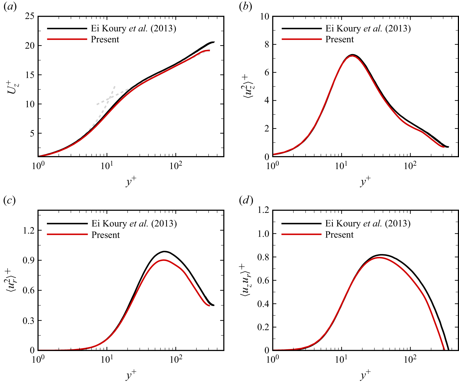
 Re=10000
 Re=11700
 Uz+
 Uz+=y+
 Uz+=k−1lny++B
 k=0.41
 B=5.2
 ⟨uz2⟩
 ⟨ur2⟩
 ⟨uzur⟩
 y+
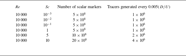
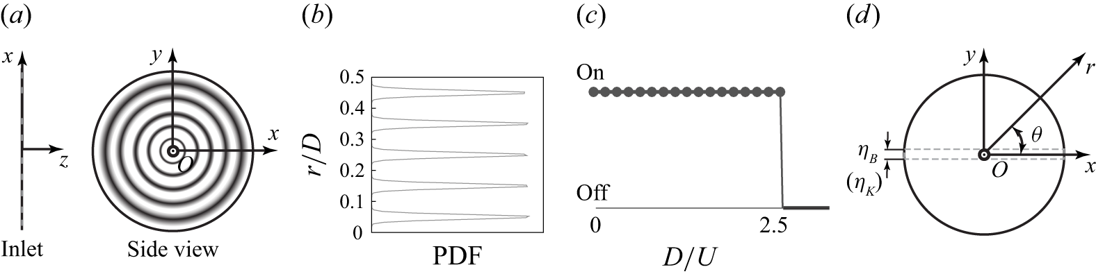
 r/D=0.05
 0.15
 0.25
 0.35
 0.45

 Re=10000
 Sc=10−3
 Sc=1
 Sc=10
 ϕ=0.12
 Sc=10−3
 z/D=3.1−3.3
 3⩽z/D⩽4

 Ruu(τ,δ)
 Rϕϕ(τ,δ)
 Sc=10−3
 Sc=1
 Sc=10
 Rϕϕ=0.96
 0.98
 Rϕϕ=0.5
 0.6
 r/D=0.3
 3⩽z/D⩽4
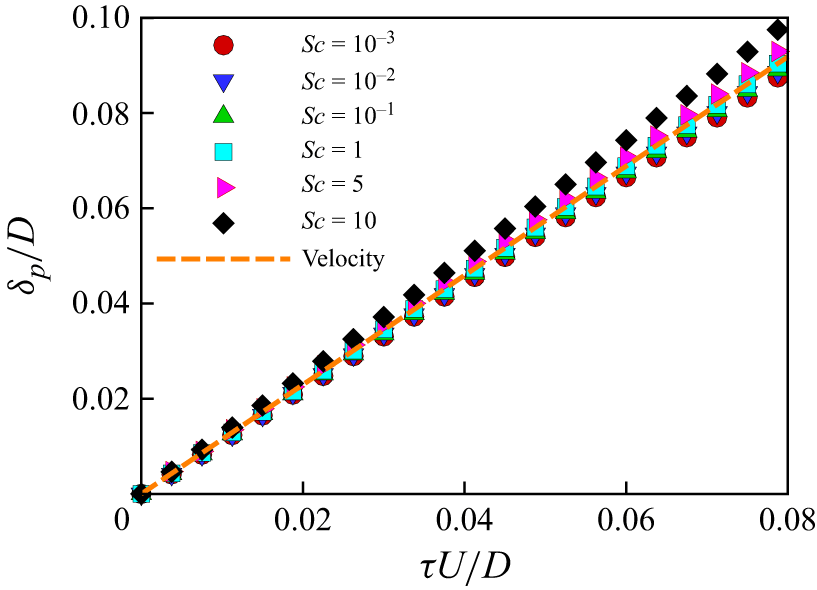
 δp/D
 τU/D
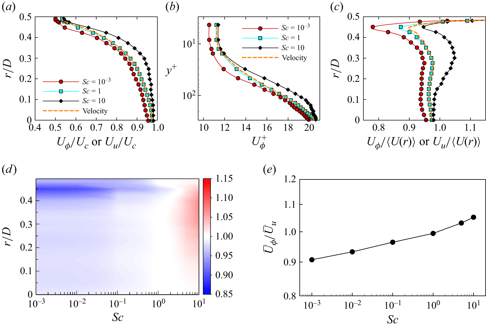
 z/D=3.5
 Uϕ/Uc
 Sc
 Uc=⟨U(r=0)⟩
 Uϕ+
 y+
 Uϕ/Uu
 U¯ϕ
 U¯u
 Sc
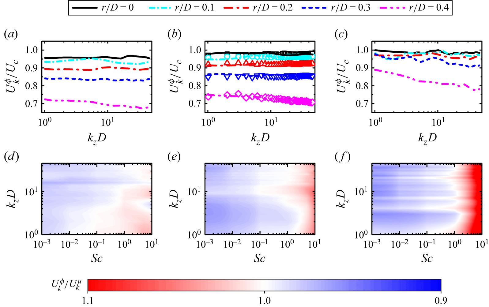
 z/D=3.5
 Ukϕ
 kzD
 Uku
 Sc=10−3
 Sc=1
 Sc=10
 Ukϕ/Uku
 Sc
 kzD
 r/D=0
 0.2
 0.4
 Sc
 Sc
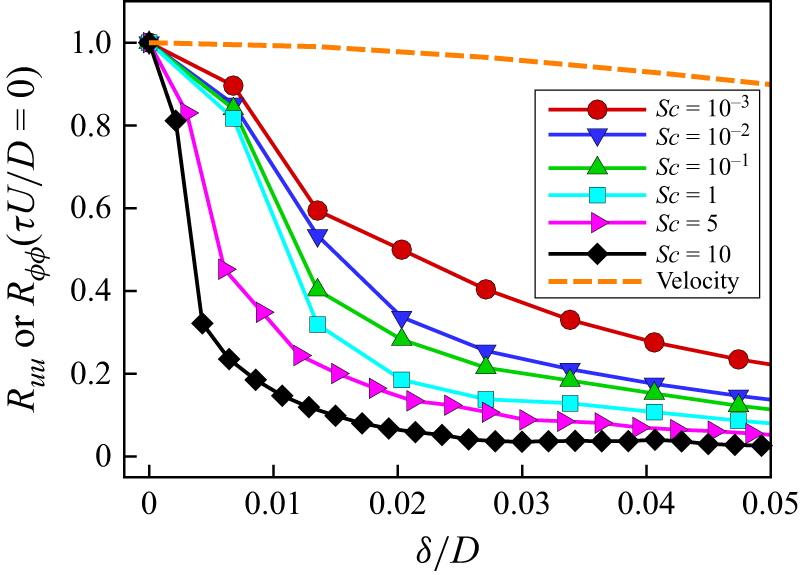
 Ruu(τU/D=0)
 Rϕϕ(τU/D=0)
 r/D=0.3
 z/D=3.5
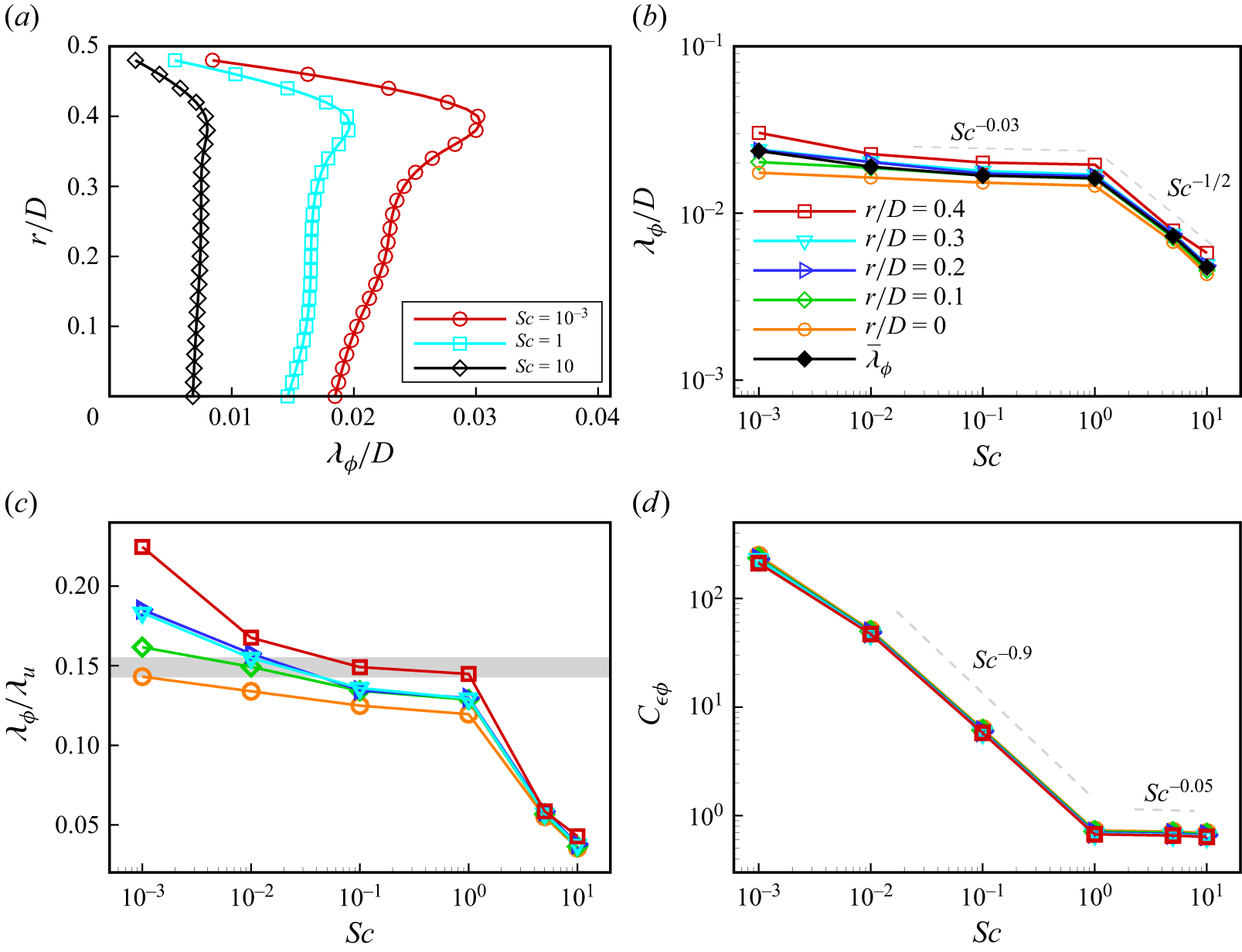
 z/D=3.5
 λϕ
 λϕ
 λ¯ϕ
 λϕ/λu
 λu
 λϕ/λu≈0.15
 Cϵϕ
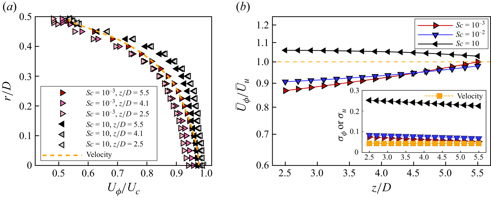
 Uϕ/Uc
 σϕ
 σu
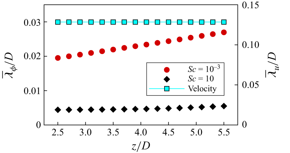
 λ¯ϕ/D
 λ¯u/D
 z/D
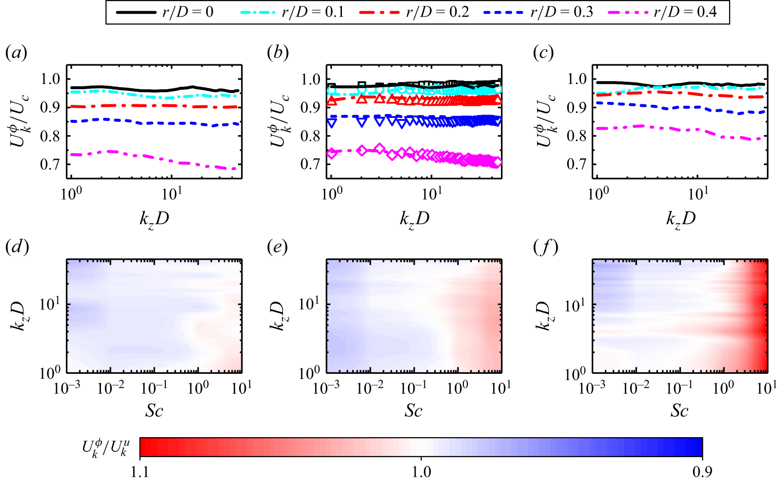
 z/D=5.5
 Ukϕ
 kzD
 Uku
 Sc=10−3
 Sc=1
 Sc=10
 Ukϕ/Uku
 Sc
 kzD
 r/D=0
 0.2
 0.4
 z/D=3.5
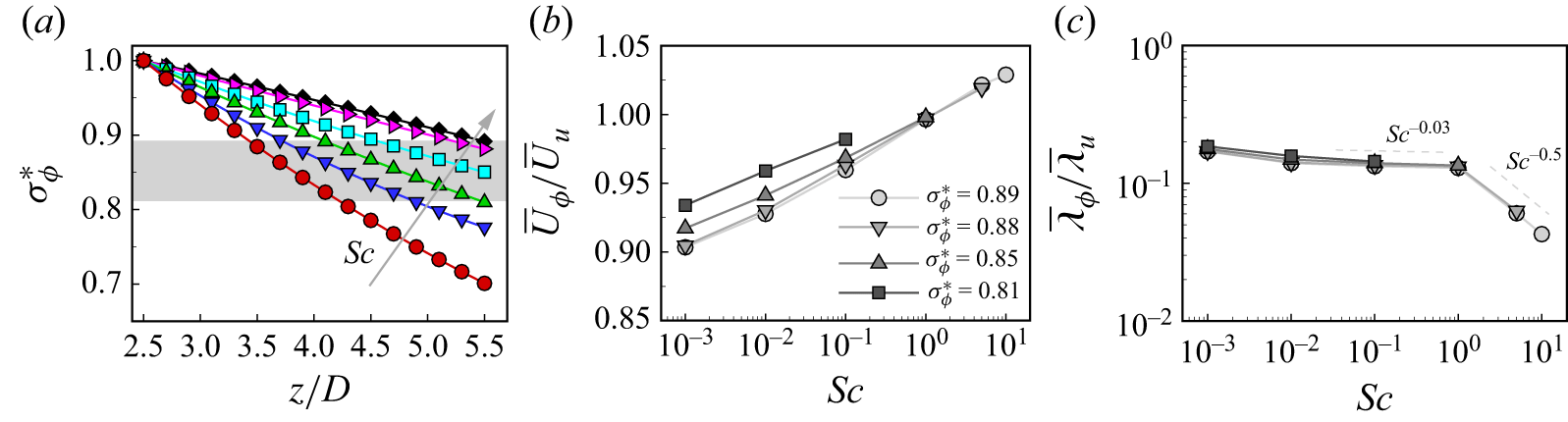
 σϕ∗=σϕ(z)/σϕ(z/D=2.5)
 σϕ∗
 Sc
 σϕ∗
 Sc
 λ¯ϕ/λ¯u
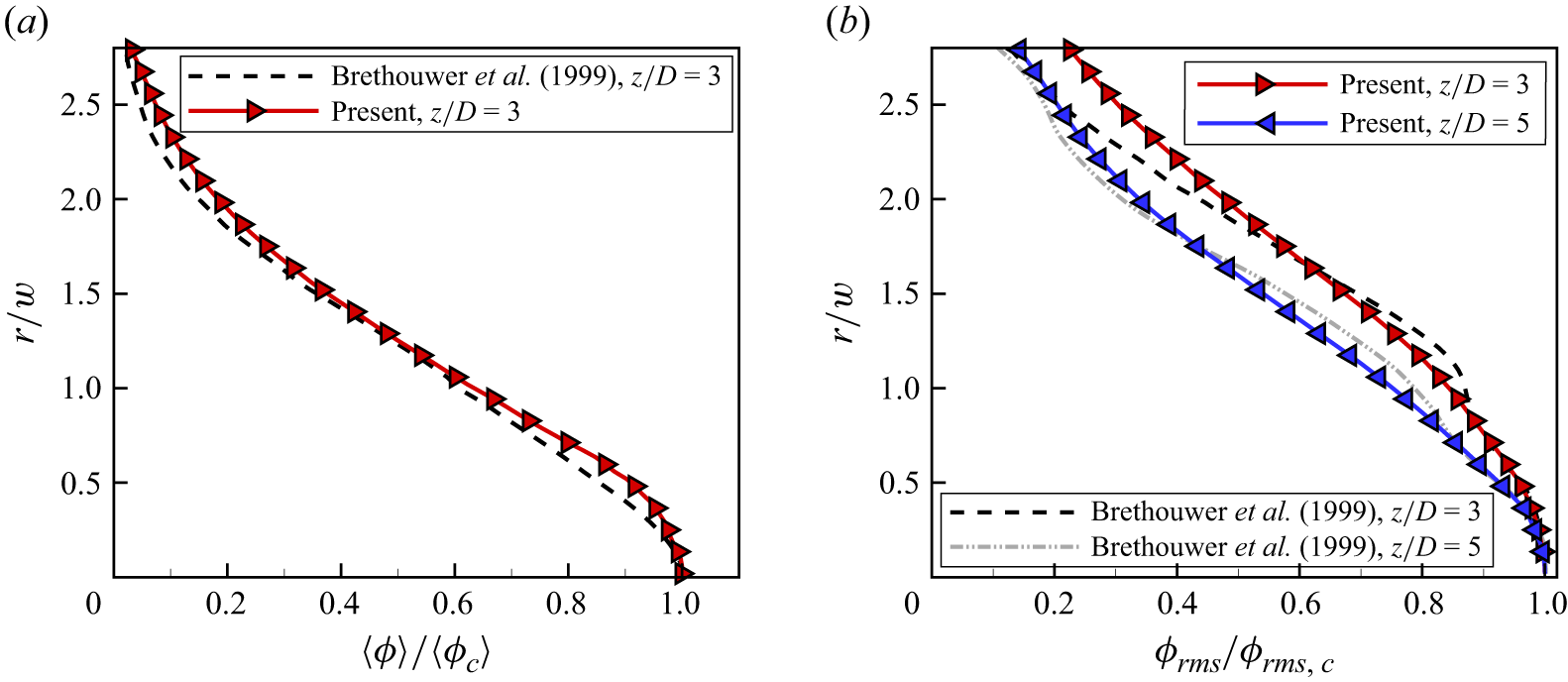
 z/D=3
 z/D=3
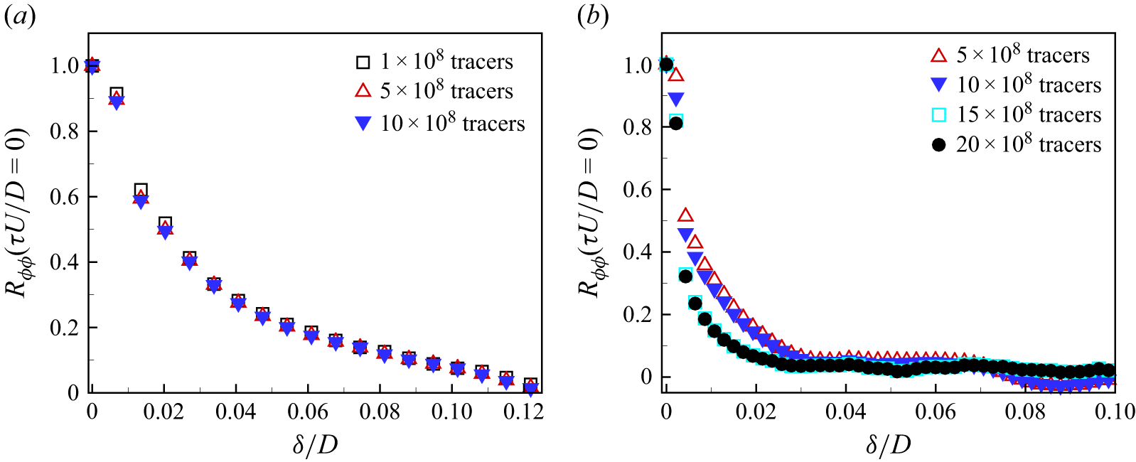
 Sc=10−3
 Sc=10
 Re=10000


