1. Introduction
Electrically charged threads hold significant application value in processes such as electrospraying, microfluidics, chemical processing, pharmaceuticals and rheometry. They are already widely utilized in inkjet printing and electrospinning, as electric fields can facilitate the generation of uniformly sized droplets and suppress drainage induced by capillary forces (Sweet Reference Sweet1965; Reneker et al. Reference Reneker, Yarin, Fong and Koombhongse2000; Hohman et al. Reference Hohman, Shin, Rutledge and Brenner2001b ; Ismail et al. Reference Ismail, Maksoud, Ghaddar, Ghali and Tehrani-Bagha2016; Wang et al. Reference Wang, Hashimoto, Li, Li and Wang2018). The coupling of electric and flow fields has resulted in new phenomena related to jet instability and breakup, and exploring the underlying mechanisms undoubtedly enriches the foundations of electrokinetics and electrohydrodynamics.
Research on electrically charged jets typically involves the application of either axial or radial electric fields. In the case of axial fields, linear stability analyses of both uncharged and charged jets (Mestel Reference Mestel1996; Saville Reference Saville1971a ) demonstrate that electric fields exert a stabilizing influence, thereby facilitating the formation of exceptionally long fibres. Hohman investigated the instability of charged viscous jets in axisymmetric and ‘whipping’ modes (Hohman et al. Reference Hohman, Shin, Rutledge and Brenner2001a , Reference Hohman, Shin, Rutledge and Brennerb ). Regarding radial electric fields, Huebner & Chu (Reference Huebner and Chu1971) conducted a linear stability analysis of perfectly conducting jets, discovering that finite disturbances are stable under long-wave conditions and unstable under short-wave conditions. Saville (Reference Saville1971b ) explored the linear stability of concentric electrodes placed at an infinite distance, while Collins, Harris & Basaran (Reference Collins, Harris and Basaran2007) examined the effects of incompatible surfaces on cylindrical electrodes at finite distances. Saville (Reference Saville1997) employed the Taylor–Melcher leaky-dielectric model to study the stability of three-dimensional dielectric fluids, while López-Herrera et al. (Reference López-Herrera, Riesco-Chueca and Gañán-Calvo2005) investigated scenarios devoid of electric effects. López-Herrera & Gañán-Calvo (Reference López-Herrera and Gañán-Calvo2004) provided numerical solutions for perfectly conducting Newtonian fluids under radial electric fields using a one-dimensional model. Collins et al. (Reference Collins, Harris and Basaran2007) explored both one-dimensional and two-dimensional models, demonstrating that electric stress significantly increases the size of satellite droplets. Additionally, Wang, Mählmann & Papageorgiou (Reference Wang, Mählmann and Papageorgiou2009) utilized a similar model to study the evolution of jets, simulating the axisymmetric nonlinear dynamics of perfectly conducting viscous liquid jets under radial electric fields. Furthermore, Conroy et al. (Reference Conroy, Craster, Matar and Papageorgiou2010) investigated the rupture of electrolyte annular liquid threads under the influence of electrostatic and electric effects in radial electric fields over finite time scales. López-Herrera & Gañán-Calvo (Reference López-Herrera and Gañán-Calvo2004) conducted experimental studies to examine the effects of viscosity and electric field strength on the size and charge of satellite droplets in perfectly conducting jets under radial electric fields. They compared their experimental results with predictions from a one-dimensional model, achieving good agreement at moderate to low electric field strengths.
Collins et al. (Reference Collins, Harris and Basaran2007) developed a robust Galerkin finite-element algorithm to solve the two-dimensional Navier–Stokes equations alongside the Laplace equation. This model controlled the axisymmetric deformation and breakup of a perfectly conducting, incompressible Newtonian fluid under a radial electric field. In another work, Wang & Papageorgiou (Reference Wang and Papageorgiou2011) studied the axisymmetric breakup of a perfectly conducting viscous liquid thread immersed in another viscous fluid using boundary integral methods, focusing on the zero Reynolds number limit. Their research highlighted the role of electric stress in stabilizing or destabilizing the liquid thread. Additionally, Wang (Reference Wang2012) extended this work to analyse poorly conducting Stokes jets suspended in a viscous medium. This study revealed that the formation of satellite droplets differs significantly from the perfectly conducting case, suggesting that electric shear stress promotes the formation of multiple satellite droplets. López-Herrera et al. (Reference López-Herrera, Gañán-Calvo, Popinet and Herrada2015) simulated the breakup of charged liquid jets, taking into account the time scales associated with diffusion and electro-osmotic migration. Lakdawala, Sharma & Thaokar (Reference Lakdawala, Sharma and Thaokar2016) introduced a dual-grid level-set method to numerically investigate the nonlinear breakup dynamics of perfectly conducting Newtonian viscous liquid jets under a radial electric field. Li et al. (Reference Li, Ke, Yin and Yin2019) discussed the influence of finite conductivity on the nonlinear dynamics of viscoelastic, weakly conducting liquid jets, concluding that tangential stress prevent the formation of satellite droplets in bead-on-string structures. Finally, Montanero & Ganan-Calvo (Reference Montanero and Ganan-Calvo2020) provided a comprehensive review of the breakup and stability analysis of charged jets, covering various experimental and theoretical developments in the field.
It has long been recognized that the presence of surfactant molecules can alter the dynamics of fluid interfaces, with numerous applications in various fields (Rodríguez-Rodríguez et al. Reference Rodríguez-Rodríguez, Sevilla, Martínez-Bazán and Gordillo2015). This influence leads to phenomena such as highly deformed drops in shear or extensional flows (Eggers Reference Eggers1997; Anna Reference Anna2016; Montanero & Ganan-Calvo Reference Montanero and Ganan-Calvo2020), as well as the formation of flower-like patterns due to the evaporation of droplets on a liquid substrate (Wodlei et al. Reference Wodlei, Sebilleau, Magnaudet and Pimienta2018). In recent years, surfactants have become one of the most compelling and widely studied factors in problems involving liquid–air and liquid–liquid interfaces. However, the underlying mechanisms remain only partially understood.
Surfactants at liquid surfaces can influence fluid dynamics through three primary mechanisms (Kamat et al. Reference Kamat, Wagoner, Thete and Basaran2018; Montanero & Ganan-Calvo Reference Montanero and Ganan-Calvo2020; Wee, Wagoner & Basaran Reference Wee, Wagoner and Basaran2022). First, the solutocapillary effect, which reduces capillary forces by lowering the surface tension coefficient. Second, the Marangoni effect, caused by an uneven distribution of surfactants along the interface, resulting in surface tension gradients. Last, surfactants induce surface rheological effects, characterized by surface shear viscosity and surface dilatational viscosity, generating additional viscous stresses.
The investigation of how factors such as capillarity, bulk viscosity, inertia, Marangoni stress and surface viscosity compete or cooperate in fluid systems is of both scientific and practical significance. Experiments and theoretical studies have demonstrated that surface viscosity plays a crucial role in various interfacial flows, such as foams (Joye, Hirasaki & Miller Reference Joye, Hirasaki and Miller1994), liquid threads (Scheid et al. Reference Scheid, Delacotte, Dollet, Rio, Restagno, van Nierop, Cantat, Langevin and Stone2010), liquid bridges (Ponce-Torres et al. Reference Ponce-Torres, Herrada, Montanero and Vega2016a ,Reference Ponce-Torres, Vega and Montanero b ) and droplet breakup (Ponce-Torres et al. Reference Ponce-Torres, Montanero, Herrada, Vega and Vega2017). Specifically, Ponce-Torres et al. (Ponce-Torres et al. Reference Ponce-Torres, Montanero, Herrada, Vega and Vega2017) concluded that surface viscosity determines the amount of surfactant retained in satellite droplets formed after pinch-off. Similarly, the effects of surface elasticity induced by the presence of surfactants have been explored in several configurations, including liquid threads (Craster, Matar & Papageorgiou Reference Craster, Matar and Papageorgiou2002; Timmermans & Lister Reference Timmermans and Lister2002), dip coating (Campana et al. Reference Campana, Ubal, Giavedoni and Saita2011; Seiwert, Dollet & Cantat Reference Seiwert, Dollet and Cantat2014; Champougny et al. Reference Champougny, Scheid, Restagno, Vermant and Rio2015), bubbles immersed in a viscous medium (Hameed et al. Reference Hameed, Siegel, Young, Li, Booty and Papageorgiou2008) and droplet deformation and breakup (Stone & Leal Reference Stone and Leal1990; Milliken, Stone & Leal Reference Milliken, Stone and Leal1993).
The linear theory has confirmed that the presence of surfactants exerts a stabilizing effect on the Rayleigh–Plateau instability of Newtonian viscous jets (Craster et al. Reference Craster, Matar and Papageorgiou2002; Ponce-Torres et al. Reference Ponce-Torres, Herrada, Montanero and Vega2016a ; Martínez-Calvo & Sevilla Reference Martínez-Calvo and Sevilla2018). This stabilizing effect manifests through a reduction in the growth rate of small perturbations, as surfactants lower the mean capillary force while introducing Marangoni stress and surface viscous stresses. Correspondingly, increasing surfactant activity or surface viscosity enhances jet stability. However, linear analysis based on the long-wave approximation cannot accurately predict certain instability characteristics, such as the cutoff wavenumber, for surfactant-laden jets and filaments without incorporating necessary higher-order terms (Timmermans & Lister Reference Timmermans and Lister2002; Martínez-Calvo & Sevilla Reference Martínez-Calvo and Sevilla2018).
Nonetheless, linear theory cannot capture the later stages of jet or filament instability. The nonlinear dynamics of Newtonian jets and filaments in the presence of surfactants have been extensively studied using asymptotic methods and numerical simulations (Craster et al. Reference Craster, Matar and Papageorgiou2002; Timmermans & Lister Reference Timmermans and Lister2002; Dravid et al. Reference Dravid, Songsermpong, Xue, Corvalan and Sojka2006; McGough & Basaran Reference McGough and Basaran2006; Craster, Matar & Papageorgiou Reference Craster, Matar and Papageorgiou2009; Hameed & Maldarelli Reference Hameed and Maldarelli2016; Martínez-Calvo et al. Reference Martínez-Calvo, Rivero-Rodríguez, Scheid and Sevilla2020; Wee et al. Reference Wee, Wagoner, Garg, Kamat and Basaran2021). These studies revealed that surfactants can delay the retraction of Newtonian liquid filaments (Craster et al. Reference Craster, Matar and Papageorgiou2002). The presence of surfactants affects the formation of satellite droplets between primary droplets, with the size of the satellite droplets increasing or decreasing depending on surfactant strength and diffusivity. Experiments and simulations by McGough & Basaran (Reference McGough and Basaran2006) and Kamat et al. (Reference Kamat, Wagoner, Thete and Basaran2018) showed that Marangoni stress near the pinching point leads to the formation of microthread cascades. When the transport of insoluble surfactants is dominated by surface convection (i.e. at high surface Péclet numbers), surfactant molecules are swept away from the pinching point (the neck of the liquid filament between primary droplets), making the behaviour of surfactant-laden jets prior to breakup similar to that of clean jets (McGough & Basaran Reference McGough and Basaran2006; Eggers & Villermaux Reference Eggers and Villermaux2008). However, even as most surfactant molecules are swept away, surface viscous stresses can still play a role because the surface-to-volume ratio at the pinching point becomes very large as the minimum jet radius approaches zero (Martínez-Calvo et al. Reference Martínez-Calvo, Rivero-Rodríguez, Scheid and Sevilla2020; Wee et al. Reference Wee, Wagoner, Garg, Kamat and Basaran2021). Moreover, surfactant molecules are not always entirely expelled from the pinching point, even at Péclet numbers as high as
 $10^5$
(Ponce-Torres et al. Reference Ponce-Torres, Rubio, Herrada, Eggers and Montanero2020).
Nonlinear analysis of one-dimensional models of surfactant-laden viscous filaments in the Stokes regime reveals the existence of a critical surface Péclet number. Below this critical value, surface diffusion dominates, and the filament thins exponentially over time; above this value, surface convection becomes dominant, and the thinning exhibits a time-dependent power-law behaviour until breakup (Wee et al. Reference Wee, Wagoner and Basaran2022). In the Stokes limit, surface viscous stresses enter the primary force balance and tend to slow the thinning of Newtonian filaments (Ozan & Jakobsen Reference Ozan and Jakobsen2019; Wee et al. Reference Wee, Wagoner, Kamat and Basaran2020). At sufficiently high surfactant surface concentrations, the balance between capillary forces and surface viscous stresses leads to exponential thinning in time, with the rate dependent solely on surface tension and surface viscosity (Martínez-Calvo & Sevilla Reference Martínez-Calvo and Sevilla2020). When inertia is considered, near the jet’s breakup point, a dominant force balance is established among inertia, capillary forces, bulk viscosity and surface viscosity, while Marangoni stress plays a secondary role (Wee et al. Reference Wee, Wagoner, Garg, Kamat and Basaran2021). Studies of surfactant effects have also been extended to compound liquid jets (Yao, Yang & Fu Reference Yao, Yang and Fu2021).
However, it is important to note that, despite many surfactants being ionic and thus influenced by electric fields, and their applications in electrohydrodynamic spraying, research on electrically driven jets containing surfactants remains relatively limited. Gallardo et al. (Reference Gallardo, Gupta, Eagerton, Jong, Craig, Shah and Abbott1999) demonstrated the use of charged surfactants to manipulate small droplets by applying an electric field. Electrified surfactants exhibit two primary effects: first, they alter surface tension; second, they influence the surface potential of the system. The surface tension results from a combination of the usual Langmuir adsorption isotherm and electrostatic contributions (Prosser & Franses Reference Prosser and Franses2001; Baygents & Saville Reference Baygents and Saville1991). In addition, charged surfactants affect both the fluid’s bulk potential and the interfacial potential, which can be represented through the Maxwell stress tensor, as studied by Conroy et al. (Reference Conroy, Craster, Matar and Papageorgiou2010, Reference Conroy, Matar, Craster and Papageorgiou2011). However, no prior research has explored the combined effects of electric forces and surface viscosity in liquid thread with charged surfactants, although surface viscosity is crucial for the dynamic analysis of liquid thread containing surfactants. This interaction introduces novel dynamical behaviours that have yet to be analysed. Therefore, in this paper, ionic surfactants and their associated surface viscosity are considered, employing the Boussinesq–Scriven model. The governing equations are non-dimensionalized and simplified under the long-wave approximation, leading to a one-dimensional model. Numerical simulations are performed to investigate the dynamics of the system.
The remainder of this paper is organized as follows. In § 2, we describe the physical model and governing equations, followed by the derivation of the simplified one-dimensional model. In § 3, we perform a linear stability analysis and present the results. Section 5 outlines the numerical methods and results. Finally, conclusions are provided in § 6.
2. Model
Consider an infinitely long axisymmetric liquid thread, surrounded by air, as depicted in figure 1. It should be noted that, in any given real-world system of charged jets, the applied electric field usually contains both radial and axial components, and the precise strength of each individual component is difficult to measure (Lakdawala et al. Reference Lakdawala, Sharma and Thaokar2016). Consequently, theoretical and numerical studies usually focus on one component of the electric field, either radial or axial. As the radial electric field is essential for elucidating the breakup modes of liquid threads and the formation of satellite droplets (Nie et al. Reference Nie, Li, Ma, Fang and Yin2021), in this study, an axisymmetric radial electric field is present outside the liquid thread, which generated by a cylindrical electrode with a radius
 $R_2$
and a uniform wall potential
 $\phi _w$
at
 $R_2$
. Prior to perturbation, the liquid thread is stationary with no underlying flow and a radius
 $R_0$
. The rheological properties, including dilatational surface viscosity and shear surface viscosity induced by surfactants, are considered. For flows with high viscosity, low velocity and small characteristic thickness, the bond number quantifying the ratio of gravity and inertia is very small, and the influence of aerodynamic forces is weak. Therefore, the hydrodynamic effects of air and gravity are neglected. An axisymmetric coordinate system
 $(r,z)$
is established, where
 $r$
represents the radial direction and
 $z$
represents the axial direction. Upon an axisymmetric harmonic perturbation being imposed, the thread starts to deform, whose radius is a function of
 $z$
and time
 $t$
, denoted by
 $r=S(z, t)$
.
Schematic diagram of a liquid thread enveloped in a radial electric field containing ionic surfactants.

Ionic surfactants are dissolved into the liquid thread and adsorped into the interface. The surface of the liquid thread is covered with the positively charged ionic surfactant of concentration
 $\varGamma$
, and the surface electric charge density is
 $q$
. Regarding the solubility of surfactants, Datwani & Stebe (Reference Datwani and Stebe1999) describes three adsorption dynamics models, among which the diffusion-controlled adsorption model is predominant under diffusion-dominated conditions, yielding the Davies adsorption isotherm at equilibrium. This study adopts the diffusion-controlled adsorption model, positing that ionic surfactants dissolve in liquid and immediately diffuse to the surface, with the characteristic time for adsorption being much shorter than the characteristic time for diffusion, and the diffusion characteristic time being significantly shorter than the characteristic time for convection. This implies a relatively small Péclet number, which is taken into account when simplifying the model in this study. In addition, the cylindrical liquid thread is a dielectric with viscosity
 $\mu _1$
, density
 $\rho _1$
and permittivity
 $\varepsilon _1$
, while the air has density
 $\rho _2$
, viscosity
 $\mu _2$
and permittivity
 $\varepsilon _2$
. The dielectric constants of the air–water system are approximately
 $\varepsilon _2/\varepsilon _1=1/80$
. In the subsequent model, the subscript
 $'1'$
denotes the liquid thread, and subscript
 $'2'$
denotes the air.
2.1. Governing equations
First, the electrostatic effects are governed by the Maxwell equations in the absence of magnetic fields,
 \begin{equation} \boldsymbol{\nabla }\boldsymbol{\cdot }(\varepsilon _i\boldsymbol{E}_i)=\rho _i^e,\quad \boldsymbol{\nabla }\times \boldsymbol{E}_i=0,\quad i=1,2, \end{equation}
where
 $\rho _i^e$
is the volume charge density within the fluid, and
 $\boldsymbol{E}_i$
is the electric field. We then introduce the electric potential
 $\phi _i$
as follows:
 \begin{equation} \boldsymbol{E}_i=-\boldsymbol{\nabla }\phi _i. \end{equation}
At the interface, electric potential must satisfy the following jump condition:
 \begin{equation} \left \| \varepsilon \boldsymbol{\nabla }\phi _i\boldsymbol{\cdot }\boldsymbol{n} \right \|=-q,\quad \left \| \boldsymbol{\nabla }\phi _i\boldsymbol{\cdot }\boldsymbol{t} \right \|=0, \end{equation}
where
 $q$
represents the surface charge density. The vectors
 $\boldsymbol{n}$
and
 $\boldsymbol{t}$
denote the unit normal (pointing outward) and unit tangential vectors, respectively. The notation
 $\left \| (\boldsymbol{\cdot }) \right \|$
represents the jump of the physical quantity
 $(\boldsymbol{\cdot })$
across the interface, defined as
 $(\boldsymbol{\cdot })_2-(\boldsymbol{\cdot })_1$
.
The electrolyte used to induce the ionic surfactant is a symmetric
 $z:z$
electrolyte. We use superscripts `
 $+$
’ and `
 $-$
’ to denote the positive and negative ions in the core flow, respectively. The concentration of positive and negative ions coming from the dissolution of surfactant in the liquid thread are represented by
 $c^{(+)}$
and
 $c^{(-)}$
, and the positive charge ions are adsorped into the interface and act as the surfactant, while
 $n^{(+)}$
and
 $n^{(-)}$
denote the ions of other electrolytes unaffected by the surfactant. The units of
 $c^{(\pm )}$
and
 $n^{(\pm )}$
are in molar concentration. The volume charge density in the core flow can then be expressed as
 \begin{equation} \rho _1^e={\textit{eN}}_A\big(n^{(+)}+c^{(+)}-n^{(-)}-c^{(-)}\big), \end{equation}
where
 $e$
is the charge on an electron, and
 $N_A$
is Avogadro’s number. And it is assumed that there is no charge in the air, i.e.
 $\rho ^e_2=0$
.
The surface charge density is given by
 \begin{equation} q={\textit{eN}}_A\big(\varGamma +n_s^{(+)}-n_s^{(-)}\big), \end{equation}
where
 $\varGamma$
represents the positively charged ionic surfactant concentration at the surface. And the surface species
 $n^{+}_s, n^{-}_s$
from other electrolytes satisfy the Nernst–Plank equation at the interface and their maximum electrolyte packing concentration is assumed to be
 $n^0_s$
(see (8), (9) and related discussion in Conroy et al. (Reference Conroy, Matar, Craster and Papageorgiou2011)).
The ion concentration in the core flow evolves according to the Nernst–Planck equation,
 \begin{equation} \frac {{\rm D}c^{(\pm )}}{{\rm D}t}=\boldsymbol{\nabla }\boldsymbol{\cdot }{\omega \big[ec^{(\pm )}\boldsymbol{\nabla }\phi _i+k_BT\boldsymbol{\nabla }c^{(\pm )}\big]}, \quad \frac {{\rm D}n^{(\pm )}}{{\rm D}t}=\boldsymbol{\nabla }\boldsymbol{\cdot }{\omega \big[e n^{(\pm )}\boldsymbol{\nabla }\phi _i+k_BT\boldsymbol{\nabla }n^{(\pm )}\big]}, \end{equation}
where
 $k_B$
is the Boltzmann constant,
 $T$
is the absolute temperature,
 $\omega$
represents the mobility of the species,
 ${\rm D}/{\rm D}t$
is the material derivative. Due to considering surfactants and other electrolytes as strong electrolytes, there are no dissociation and association terms for ions in (2.6). In addition, the equilibrium condition in the thread satisfies where the electric potential
 $\phi _1=\phi ^0$
(assuming
 $\phi ^0=0$
) and the corresponding total positive and negative ion concentrations are both
 $c_0$
.
At the interface, the concentration
 $\varGamma$
of the positively charged surfactants evolves according to the following evolution equation:
 \begin{equation} \frac {\partial \varGamma }{\partial t}-\frac {\partial \boldsymbol{X}}{\partial t}\boldsymbol{\nabla\!}_s\varGamma +\boldsymbol{\nabla\!}_s\boldsymbol{\cdot }(\varGamma \boldsymbol{u}_t)+\varGamma \zeta \boldsymbol{u}\boldsymbol{\cdot }\boldsymbol{n}=\boldsymbol{\nabla\!}_s\boldsymbol{\cdot }(D_s\boldsymbol{\nabla\!}_s\varGamma +D_{s\phi }\varGamma \boldsymbol{\nabla\!}_s\phi _s), \end{equation}
where
 $\partial \varGamma /\partial t$
is the time derivative following the evolution of the surface point by keeping the surface coordinates fixed,
 $\boldsymbol{X}$
is the position vector of the surface point,
 $\boldsymbol{\nabla\!}_s=(\boldsymbol{I}-\boldsymbol{nn})\boldsymbol{\cdot }\boldsymbol{\nabla}$
is the surface gradient operator,
 $\boldsymbol{u}$
is the velocity of the surface point and
 $\boldsymbol{u}_t$
is the tangential component of velocity for the corresponding surface point,
 $\zeta =\boldsymbol{\nabla }\boldsymbol{\cdot }\boldsymbol{n}$
is the curvature at the interface,
 $D_s$
is the surface diffusion coefficient,
 $D_{s\phi }=D_s e/k_B T$
is the diffusion coefficient for ion migration and
 $\phi _s$
is the electric potential at the interface. The above evolution equation is based on the book chapter (Papageorgiu Reference Papageorgiu2002), where the ion electromigration term is obtained by assuming
 $J_{\phi }\,D_{s\phi }\boldsymbol{\nabla\!}_s\phi _s$
. And here we make the equilibrium assumption for low concentrations and ignore surface flux to the interface from the bulk fluid (Conroy et al. Reference Conroy, Matar, Craster and Papageorgiou2011). This study considers the case where the surfactant concentration does not reach the critical micelle concentration.
The continuity equation and Navier–Stokes equations for the fluid can be written as follows:
 \begin{align}&\qquad\quad \boldsymbol{\nabla }\boldsymbol{\cdot }\boldsymbol{u}_i=0,\quad i=1,2, \end{align}
 \begin{align}& \rho _i\frac {{\rm D}\boldsymbol{u}_i}{{\rm D}t}=\boldsymbol{\nabla }\boldsymbol{\cdot }\big(\boldsymbol{T}_i^f+\boldsymbol{T}_i^e\big),\quad i=1,2. \end{align}
Assuming the fluid is incompressible, the fluid stress tensor and Maxwell stress tensor appearing in (2.9) can be given as follows:
 \begin{align}&\qquad \boldsymbol{T}_i^f=-p_i\boldsymbol{I}+\boldsymbol{\tau }_i, \end{align}
 \begin{align}& \boldsymbol{T}_i^e=\varepsilon _i\left(\boldsymbol{E}_i\boldsymbol{E}_i-\frac {1}{2}|\boldsymbol{E}_i|^2\boldsymbol{I}\right)\!. \end{align}
Here,
 $p_1$
is pressure of the liquid thread,
 $p_2$
is air pressure,
 $\boldsymbol{\tau }_i=\mu _i[\boldsymbol{\nabla }\boldsymbol{u}_i+(\boldsymbol{u}_i)^{\textrm {{T}}}]$
and
 $\boldsymbol{\nabla }\boldsymbol{\cdot }T_i^e=\rho _i^e\boldsymbol{E}_i$
.
The boundary conditions can be summarized as kinematic boundary conditions and dynamic boundary conditions. The first is the no-slip boundary condition, with
 $\boldsymbol{u}_2(R_2,z,t)=\textbf {0}$
at the pipe wall. In addition, there is a continuity of velocity at the gas–liquid interface,
 \begin{equation} \left \| \boldsymbol{u}_i \right \|=0, \end{equation}
where
 $\boldsymbol{u}_i=(u_i, w_i)^T$
,
 $w_i$
represents the axial velocity (
 $z$
direction) and
 $u_i$
represents the radial velocity (
 $r$
direction).
The movement of the position of the gas–liquid interface conforms to the kinematic boundary conditions,
 \begin{equation} u_i=S_t+w_iS_z, \end{equation}
where the velocity term is calculated at the interface.
 $S_t$
denotes the partial derivative of
 $S$
with respect to time and
 $S_z$
denotes the partial derivative of
 $S$
with respect to
 $z$
.
In this model, it is assumed that surfactants induce both surface elasticity and surface viscosity at the gas–liquid interface. In other words, it not only reduces surface tension but also causes additional viscous stresses at the interface, as described by Martínez-Calvo & Sevilla (Reference Martínez-Calvo and Sevilla2018). The free-surface stress is simulated by two surface viscosities: surface shear viscosity
 $\mu _s(\varGamma )$
and dilatational viscosity
 $\kappa _s(\varGamma )$
. Following the derivation process of Martinez-Calvo & Sevilla (Reference Martínez-Calvo and Sevilla2018), the stress balance at the gas–liquid interface can be expressed as follows:
 \begin{equation} \big \| \boldsymbol{T}_i^f+\boldsymbol{T}_i^e \big \|\boldsymbol{\cdot }\boldsymbol{n}+\boldsymbol{\nabla\!}_s\boldsymbol{\cdot }\boldsymbol{T\!}_s=0, \end{equation}
where the surface stress tensor
 $\boldsymbol{T\!}_s$
is defined using the well-known Boussinesq–Scriven approximation, which neglects surface density and simplifies the complex interfacial rheology. This approximation assumes that the deviatoric components of
 $\boldsymbol{T\!}_s$
are isotropic, linear and instantaneous in the surface strain rate tensor (Boussinesq Reference Boussinesq1913; Scriven & Sternling Reference Scriven and Sternling1960),
 \begin{equation} \boldsymbol{T\!}_s=\boldsymbol{I}_s[\sigma +(\kappa _s-\mu _s)(\boldsymbol{\nabla\!}_s\boldsymbol{\cdot }\boldsymbol{u}_s)]+\mu _s\left[(\boldsymbol{\nabla\!}_s\boldsymbol{u}_s)\boldsymbol{\cdot }\boldsymbol{I}_s+\boldsymbol{I}_s(\boldsymbol{\nabla\!}_s\boldsymbol{u}_s)^{\textrm {T}}\right]\!. \end{equation}
Substituting the (2.15) into (2.14) yields
 \begin{equation} \begin{aligned} &\big \| \boldsymbol{T}_i^f+\boldsymbol{T}_i^e \big \|\boldsymbol{\cdot }\boldsymbol{n}+\boldsymbol{\nabla\!}_s\sigma -\boldsymbol{n}(\boldsymbol{\nabla\!}_s\boldsymbol{\cdot }\boldsymbol{n})\sigma +\boldsymbol{\nabla\!}_s[(\kappa _s-\mu _s)(\boldsymbol{\nabla\!}_s\boldsymbol{\cdot }\boldsymbol{u}_s)] \\ &\quad -\boldsymbol{n}(\boldsymbol{\nabla\!}_s\boldsymbol{\cdot }\boldsymbol{n})(\kappa _s-\mu _s)(\boldsymbol{\nabla\!}_s\boldsymbol{\cdot }\boldsymbol{u}_s)+\boldsymbol{\nabla\!}_s\boldsymbol{\cdot }\left \{ {\mu _s\left[(\boldsymbol{\nabla\!}_s\boldsymbol{u}_s)\boldsymbol{\cdot }\boldsymbol{I}_s+\boldsymbol{I}_s\boldsymbol{\cdot }(\boldsymbol{\nabla\!}_s\boldsymbol{u}_s)^{\textrm {T}}\right]} \right \}=0, \end{aligned} \end{equation}
where
 $\zeta =\boldsymbol{\nabla\!}_s\boldsymbol{\cdot }\boldsymbol{n}= {1}/{S\sqrt {1+S_z^2}}- {S_{\textit{zz}}}/{\sqrt {(1+S_z^2)^3}}$
is mean curvature of the interface.
The velocity field on the surface of the fluid,
 $\boldsymbol{u}_s$
, can be decomposed into two components: tangential velocity
 $\boldsymbol{u}_t$
and normal velocity
 $\boldsymbol{u}_n$
,
 \begin{equation} \boldsymbol{u}_s=\boldsymbol{u}(\boldsymbol{X},t)=\boldsymbol{u}_t(\boldsymbol{X},t)+\boldsymbol{u}_n(\boldsymbol{X},t)=\boldsymbol{u}_t(\boldsymbol{X},t)+u_n(\boldsymbol{X},t)\boldsymbol{n}, \end{equation}
where
 $\boldsymbol{u}_t=\boldsymbol{I}_s\boldsymbol{\cdot }\boldsymbol{u}_s$
,
 $\boldsymbol{u}_n=\boldsymbol{n}\boldsymbol{n}\boldsymbol{\cdot }\boldsymbol{u}_s$
and
 $\boldsymbol{I}_s=\boldsymbol{I}-\boldsymbol{n}\boldsymbol{n}$
is surface projection operator. Since the interface is axisymmetric, we have
 $\boldsymbol{u}_t=u_t(\boldsymbol{X},t)\boldsymbol{t}$
, and then the normal and tangential velocity at the interface can be written as follows:
 \begin{equation} u_n=\frac {u-S_z w}{\sqrt {1+S_z^2}},\quad u_t=\frac {w+S_z u}{\sqrt {1+S_z^2}}, \end{equation}
where
 $\boldsymbol{u}_s=(u,w)^{\text{T}}$
,
 $u$
and
 $w$
are the radial and axial components of fluid velocity on the interface, respectively. In light of the aforementioned equations,
 $\boldsymbol{\nabla\!}_s\boldsymbol{\cdot }\boldsymbol{u}_s=\boldsymbol{\nabla\!}_s\boldsymbol{\cdot }\boldsymbol{u}_t+\zeta u_n$
can be applied to (2.16).
Taking the inner product for both sides of (2.16) with
 $\boldsymbol{n}$
and
 $\boldsymbol{t}$
, respectively, yields the normal and tangential boundary conditions at the interface,
 \begin{equation} \begin{aligned} &-\!\left \| p_i-\frac {2\mu _i}{1\!+\!S_z^2}\left[u_r-S_z(u_z+w_r)+\!S_z^2w_z\right] \right \|\!+\!\left \| \frac {\varepsilon _i}{2}\frac {1\!-\!S_z^2}{1\!+\!S_z^2}(\phi _{\textit{ir}}^2-\phi _{\textit{iz}}^2)-2\varepsilon _i\frac {S_z^2}{1\!+\!S_z^2}\phi _{\textit{ir}}\phi _{\textit{iz}} \right \|\\&=\zeta \!\left [\! \sigma +(\kappa _s-\mu _s)\!\left ( \!\frac {({\textit{Su}}_t)_z}{S\sqrt {1\!+\!S_z^2}}+\zeta u_n \!\right )\! \right ] +\frac {2\mu _s}{1\!+\!S_z^2}\!\left [ \!\frac {S_z u_t\!+u_n}{S^2}-\frac {S_{\textit{zz}}}{1\!+\!S_z^2}\!\left ( \!\frac {\partial u_t}{\partial z}-\frac {S_{\textit{zz}}u_n}{1\!+\!S_z^2} \!\right ) \!\right ]\!, \end{aligned} \end{equation}
 \begin{align} &-\frac {1}{\sqrt {1+S_z^2}}\left \| 2\mu _i\left [ u_r S_z+\frac {1}{2}(1-S_z^2)(u_z+w_r)-S_z w_z \right ] \right \|+\frac {2\beta }{\sqrt {1+S_z^2}} q(S_z\phi _{i,r}+\phi _{i,z})|_{S} \nonumber\\& =\frac {\partial \sigma }{\partial z}+\frac {\partial }{\partial z}\!\left [\! (\kappa _s-\mu _s)\!\left ( \!\frac {({\textit{Su}}_t)_z}{S\sqrt {1\!+\!S_z^2}}+\zeta u_n \!\right )\! \right ]+\frac {\sqrt {1\!+\!S_z^2}}{S}\frac {\partial }{\partial z}\!\left [ \!\frac {2\mu _s S}{\sqrt {1\!+\!S_z^2}}\!\left ( \!\frac {\partial u_t}{\partial z}-\frac {S_{\textit{zz}}u_n}{1\!+\!S_z^2} \!\right ) \!\right ] \nonumber\\ &\quad -\frac {2\mu _s S_z}{\sqrt {1+S_z^2}}\left [ \frac {S_z u_t+u_n}{S^2}-\frac {S_{\textit{zz}}}{1+S_z^2}\left ( \frac {\partial u_t}{\partial z}-\frac {S_{\textit{zz}}u_n}{1+S_z^2} \right )\right ]\!, \\[9pt] \nonumber \end{align}
where the subscripts ‘
 $r$
’ and ‘
 $z$
’ represent the partial derivative.
It should be noted that both the surface shear viscosity
 $\mu _s(\varGamma )$
and the dilatational viscosity
 $\kappa _s(\varGamma )$
are functions of the surfactant concentration
 $\varGamma$
at the interface. It can be assumed that
 $\mu _s(\varGamma )$
and
 $\kappa _s(\varGamma )$
are linearly dependent on
 $\varGamma$
(Martínez-Calvo & Sevilla Reference Martínez-Calvo and Sevilla2018), that is
 \begin{equation} \kappa _s(\varGamma )=\kappa _{\textit{sr}}\frac {\varGamma }{\varGamma _r},\quad \mu _s(\varGamma )=\mu _{\textit{sr}}\frac {\varGamma }{\varGamma _r}, \end{equation}
where the
 $\varGamma _r$
represents the reference point for the surfactant concentration,
 $\kappa _{\textit{sr}}$
and
 $\mu _{\textit{sr}}$
are two constants.
Furthermore, expression of surface tension under an electrical field is elucidated, which is a function of the surfactant concentration and the interfacial electric potential. Prosser & Franses (Reference Prosser and Franses2001) has provided the formula for calculating the surface tension in the case of over equilibrium, utilizing the chemical potential and the Gibbs adsorption equation. Datwani & Stebe (Reference Datwani and Stebe1999) has also delineated the impact of an excess Maxwell stress on the surface tension generated by the electric potential on the surface. The aforementioned studies have demonstrated that the surface tension can be expressed as the sum of the contributions from the Langmuir isotherms and the electrical effect,
 \begin{equation} \sigma =\sigma _0+R_g T\varGamma _{\infty }\rm {ln}\left(1-\frac {\varGamma }{\varGamma _{\infty }}\right)+\int _0^{\phi _s}qd\phi , \end{equation}
where
 $\sigma _0$
denotes the surface tension of the cleaning interface,
 $\varGamma _{\infty }$
denotes the maximum packing surfactant concentration and
 $R_g$
is the gas constant.
2.2. One-dimensional model
In light of the elongated thread, the radial reference size
 $R_0$
is considerably smaller than the axial reference size
 $L$
, rendering the one-dimensional model analysis a viable approach. As the outside of the thread is air, whose viscosity is much smaller than the liquid, and air pressure can be assumed to be a constant, under the condition that the maximum electrolyte packing concentration
 $n^0_s$
from other electrolytes is far less than the surfactant maximum packing concentration
 $\varGamma _{\infty }$
on the interface, we can derive the one-dimensional long-wave model similar as in Conroy et al. (Reference Conroy, Matar, Craster and Papageorgiou2011). The specific derivation process of the one-dimensional model is outlined in Appendix A.
By choosing the unperturbed radius of the thread
 $R_0$
as the length scale,
 $\sigma _0/\mu _1$
as the velocity scale,
 $R_0\mu _1/\sigma _0$
as the time scale,
 $\sigma _0/R_0$
as the pressure scale,
 $k_BT/e$
as the electric potential scale,
 $2\varGamma _{\infty }e N_A$
as scale for the charge density and
 $\varGamma _{\infty }$
as the scale for surfactant concentration, the final dimensionless one-dimensional equations are as follows:
 \begin{align}&\qquad\qquad\qquad q_t+q_z w+\frac {1}{2}qw_z=\frac {{\textit{Pe}}_s^{-1}}{S}\frac {\partial }{\partial z}(Sq_z+Sq\phi _{s,z}), \end{align}
 \begin{align}& \left [ \frac {S}{2}Re(w_t+{ww}_z)-3S_z w_z-\frac {3}{2}{\textit{S}w}_{\textit{zz}} \right ]\nonumber\\ &\qquad + \frac {S}{4}Q\left \{ \chi ^2\phi _s^2\left [ \frac {I_1^2(\chi S)}{I_0^2(\chi S)}-1 \right ] -\frac {\varepsilon _2}{\varepsilon _1}\left [ \frac {\phi _s-\phi _w}{S\ln (R_2/S)} \right ]^2 \right \}_z+2\beta q\phi _{s,z} \nonumber\\ &\quad =\left [ \sigma +q({\textit{Bo}}_{\kappa \infty }-{\textit{Bo}}_{\mu \infty })\left ( \frac {(\textit{S}w)_z}{S}+\zeta (-\frac {{\textit{S}w}_z}{2}-S_zw) \right ) \right ]_z \nonumber\\ &\qquad \quad \unicode{x2460}\quad \quad \quad \quad \quad \quad \quad \unicode{x2461} \nonumber\\ &\qquad -\frac {S}{2}\left \{ \zeta \left [ \sigma +q({\textit{Bo}}_{\kappa \infty }-{\textit{Bo}}_{\mu \infty })\left ( \frac {({\textit{S}w})_z}{S}+\zeta (-\frac {{\textit{S}w}_z}{2}-S_zw) \right ) \right ] \right \}_z \nonumber\\ &\qquad \quad \quad \quad \quad \unicode{x2462} \quad \quad \quad \quad \quad \unicode{x2463} \nonumber\\ &\qquad +\frac {5{\textit{Bo}}_{\mu \infty }}{2S}\boldsymbol{\cdot }\frac {\partial }{\partial z}[q{\textit{S}w}_z], \nonumber\\ &\quad \quad \quad \unicode{x2464} \end{align}
 \begin{align}&\qquad\qquad\qquad\qquad\qquad S_t+{w\textit{S}}_z+\frac {1}{2}{\textit{S}w}_z=0, \end{align}
where
 \begin{align}& \sigma =1+\beta \ln (1-2q)+\beta q\phi _s-\beta \frac {(\varepsilon _2/\varepsilon _1)\phi _w}{\chi ^2\xi S\ln (R_2/S)}(\phi _s-\varPhi ),\\[-12pt] \nonumber \end{align}
 \begin{align}&\quad\,\, \phi _s=I_0(\chi S)\frac {\chi ^2\xi qS\ln (R_2/S)+(\varepsilon _2/\varepsilon _1)\phi _w}{\chi I_1(\chi S)S\ln (R_2/S)+(\varepsilon _2/\varepsilon _1)I_0(\chi S)},\\[-12pt] \nonumber \end{align}
 \begin{align}&\qquad\qquad \varPhi =\frac {(\varepsilon _2/\varepsilon _1)\phi _w}{\varepsilon _2/\varepsilon _1+\chi \frac {I_1(\chi S)}{I_0(\chi S)}S\ln (R_2/S)},\\[-12pt] \nonumber \end{align}
 \begin{align}&\qquad\qquad\,\, \zeta =\frac {1}{S\sqrt {1+S_z^2}}-\frac {S_{\textit{zz}}}{\sqrt {(1+S_z^2)^3}}.\\[-12pt] \nonumber \end{align}
The one-dimensional model presented above comprises three independent variables:
 $q$
represents the surface charge density, which is related to the surfactant concentration,
 $q=( {1}/{2})\varGamma$
with initial values of
 $q_0$
and
 $\Gamma_0$
, respectively;
 $w$
represents the axial velocity, with an initial value of
 $0$
; and
 $S$
indicates the position of the gas–liquid interface.
Equation (2.23) represents the transport equation for the surface charge, with the convection term on the left-hand side and the diffusion term on the right-hand side. Equation (2.24) is a one-dimensional momentum equation. The second and third terms on the left-hand side of the equation represent the electrostatic stress in the bulk stream and the electrostatic tension from the tangential stress equilibrium, respectively. On the right-hand side of this equation, term ① represents the Marangoni stress caused by the spatial inhomogeneity of surface tension and the electrical effect, term ③ is the capillary stress, and terms ②, ④ and ⑤ represent the surface viscous stresses associated with surface dilatational deformation and surface shear deformation.
The dimensionless numbers that appear in the above one-dimensional model are as follows: the Péclet number on the interface
 ${\textit{Pe}}_s=(\sigma _0 R_0)/(D_s \mu )$
, the Reynolds number
 ${\textit{Re}}=(\rho \sigma _0R_0)/(\mu ^2)$
, the electrostatic Weber number
 $Q=(\varepsilon _1 k_BT/e)/(\sigma _0 R_0)$
characterizing the ratio of electrostatic stress to capillary stress, the Marangoni number
 $\beta =R_g T\varGamma _{\infty }/\sigma _0$
quantifying the sensitivity of surface tension to surfactant concentration, the dilatational Boussinesq number
 ${\textit{Bo}}_{\kappa \infty }=(2\kappa _{\textit{sr}}\varGamma _{\infty })/(\mu _1 R_0 \varGamma _r)$
and the shear Boussinesq number
 ${\textit{Bo}}_{\mu \infty }=(2\mu _{\textit{sr}}\varGamma _{\infty })/(\mu _1 R_0 \varGamma _r)$
used to characterize the relative importance of surface viscosity versus bulk viscosity. Here, an additional parameter
 $\varTheta = \kappa _s/\mu _s={\textit{Bo}}_{\kappa \infty }/{\textit{Bo}}_{\mu \infty }$
is introduced to represent the dilatational-to-shear surface viscosity ratio. The remaining parameters in the one-dimensional model are as follows:
 $\chi =\sqrt {(2R_0^2 e^2 c_0 N_A)/(k_B T\varepsilon _1)}$
represents the ratio of the radius of the liquid thread to the length of Debye,
 $\xi =\varGamma _{\infty }/(c_0 R_0)$
is related to the concentration of surfactant and ions in the mainstream, and
 $\phi _s$
is the electric potential at the gas–liquid interface.
For an isothermal saturated interface, the Marangoni stress can be neglected, and the only relevant surface stresses are the Young–Laplace pressure and surface viscous stresses (Quéré & de Ryck Reference Quéré and de Ryck1998; Scheid et al. Reference Scheid, Delacotte, Dollet, Rio, Restagno, van Nierop, Cantat, Langevin and Stone2010; Scheid et al. Reference Scheid, Dorbolo, Arriaga and Rio2012; Martínez-Calvo & Sevilla Reference Martínez-Calvo and Sevilla2020). Martinez–Calvo provided a detailed description of the applicable conditions, and as discussed by Quéré & de Ryck (Reference Quéré and de Ryck1998) in the context of axisymmetric flows, the validity of the assumption is ensured if two conditions are met: first, there must be sufficient surfactant available at the interface during the thinning process; second, the adsorption rate must exceed the characteristic velocity of the interface. This aligns with the diffusion-controlled model and the small Péclet number assumption used in this paper. Furthermore, when the surfactant concentration is low, the influence of the Marangoni effect can similarly be neglected (Ponce-Torres et al. Reference Ponce-Torres, Montanero, Herrada, Vega and Vega2017), as its impact on the surface tension coefficient is minimal. In addition, the surface viscosity coefficient is difficult to measure under significant Marangoni stress and adsorption dynamics, as all these effects are inherently entangled (Prosser & Franses Reference Prosser and Franses2001; Elfring, Leal & Squires Reference Elfring, Leal and Squires2016). Therefore, although the Marangoni effect was considered during the derivation process, it was neglected in the result calculations, which means
 $\beta =0$
. This decision is based on two reasons: first, under the aforementioned applicable conditions, neglecting the Marangoni effect is reasonable; second, more importantly, it serves to highlight the influence of surface viscosity, allowing for a more in-depth study of the mechanisms by which surface viscosity and electric effects influence the instability of liquid jets.
If the concentration of the surfactant is set to zero, that is to say the density of the surface charge is also set to zero, then the surface viscosity will also be absent. If the surface viscosity be set to zero, the one-dimensional model will degenerate into the model of Conroy et al. (Reference Conroy, Matar, Craster and Papageorgiou2011).
3. Linear instability analysis
The influence of dimensionless parameters on the dispersion relation is a significant result. Indeed, there are certain dimensionless parameters that have been the subject of prior investigation. Papageorgiu (Reference Papageorgiu2002) investigated the impact of surfactants and Reynolds numbers, while Conroy et al. (Reference Conroy, Matar, Craster and Papageorgiou2011) examined the influence of electrostatic and electrokinetic effects, including the electrostatic Weber numbers
 $Q$
,
 $\chi$
,
 $\xi$
and so forth, without accounting for surface viscosity. Martínez-Calvo & Sevilla (Reference Martínez-Calvo and Sevilla2018) investigated the impact of surface viscoelasticity induced by surfactants, encompassing dimensionless parameters such as
 $\beta$
,
 ${\textit{Bo}}_{\kappa \infty }$
,
 ${\textit{Bo}}_{\mu \infty }$
and others. Li & He (Reference Li and He2023) conducted a study on the kinetic characteristics of viscoelastic threads containing surfactants and provided a summary of the dimensionless parameters that had been previously selected in studies of surfactant-laden fluids. Among these parameters, the values of Boussinesq numbers were identified as being of particular significance for this paper.
In light of the aforementioned considerations, an investigation is conducted into the combined influence of surface charge density and surface viscosity. Consequently, the initial surface charge density,
 $q_0$
, and the Boussinesq numbers,
 ${\textit{Bo}}_{\kappa \infty }$
and
 ${\textit{Bo}}_{\mu \infty }$
, are the primary variables under consideration. In the absence of special instructions, the following parameters are selected in this section and § 5: interface Péclet number
 ${\textit{Pe}}_s=10$
, Reynolds number
 ${\textit{Re}}=1$
, electrostatic Weber number
 $Q=2$
, Marangoni number
 $\beta =0$
(no Marangoni effect), ratio of liquid thread radius to Debye length
 $\chi =1.5$
, ratio of surfactant concentration to mainstream ion concentration
 $\xi =0.1$
, wall potential
 $\phi _w=2$
, wall radius
 $R_2=5$
and dielectric constant ratio
 $\varepsilon _2/\varepsilon _1=1/80$
.
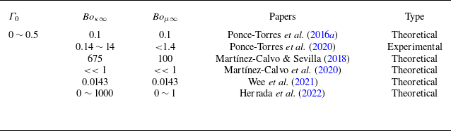
The initial surface charge density and Boussinesq numbers were selected based on the parameter values presented in the surveyed literature, which are listed in table 1. In consideration of the parameter values presented in the aforementioned articles, it can be inferred that the range of surface charge density is
 $0{\sim}0.25$
based on
 $q_0=\varGamma _0/2$
, while the range of Boussinesq numbers is
 $0{\sim}100$
.
The range of surfactant concentrations and the corresponding physical property parameters presented in these literatures when the critical micelle concentration is not reached.

The solution to the dispersion relation for the above one-dimensional system (2.23)–(2.25) can be transformed into solving a generalized eigenvalue problem as shown in (3.1),
 \begin{equation} \begin{gathered} \boldsymbol{A} \begin{bmatrix} \hat {q} \\ \hat {S} \\ \hat {w} \end{bmatrix} =\lambda \boldsymbol{B} \begin{bmatrix} \hat {q} \\ \hat {S} \\ \hat {w} \end{bmatrix}\!, \end{gathered} \end{equation}
where
 $\lambda$
is the growth rate of the perturbation, and
 $\boldsymbol{A}$
and
 $\boldsymbol{B}$
are the coefficient matrices. The derivation process is detailed in Appendix B.
Based on the currently selected parameter range, further simplification of (3.1) yields the approximate solution
 \begin{equation} \lambda =\frac {-[6+(9+\varTheta )q_0{\textit{Bo}}_{\mu \infty }]k^2+\sqrt {[6+(9+\varTheta )q_0{\textit{Bo}}_{\mu \infty }]^2k^4+8(k^2-k^4)Re}}{4{\textit{Re}}}, \end{equation}
where
 $k$
is the axial wavenumber. It should be noted that this approximate solution is primarily used to provide a more intuitive understanding of the influence of key parameters on the growth rate. We still prioritize the numerical results obtained from solving (3.1). A comparison between the approximate and numerical solutions is presented in figure 2( f), where the discrepancy is insignificant, thereby validating the accuracy of the approximate solution.
The relation between the growth rate
 $\lambda$
and the axial wavenumber
 $k$
. The effect of (a) the initial surface charge density
 $q_0$
, with
 ${\textit{Bo}}_{\kappa \infty }={\textit{Bo}}_{\mu \infty }=1$
, (b) the dilatational Boussinesq number
 ${\textit{Bo}}_{\kappa \infty }$
, with
 ${\textit{Bo}}_{\mu \infty }=0,q_0=0.075$
, (c) the shear Boussinesq number
 ${\textit{Bo}}_{\mu \infty }$
, with
 ${\textit{Bo}}_{\kappa \infty }=0,q_0=0.075$
and (d) the dilatational-to-shear surface viscosity ratio
 $\varTheta$
for
 ${\textit{Bo}}_{\mu \infty } = 0.1, q_0=0.075$
. (e) Changing
 $\varTheta$
or
 ${\textit{Bo}}_{\mu \infty }$
can produce similar effects on the dispersion relation, with
 $q_0=0.075$
. ( f) Comparison between the approximate solution (3.2) and the numerical solution (3.1).

Figure 2 illustrates the impact of the initial surface charge density and the two Boussinesq numbers on the dispersion relation, where figure 2(a–e) are obtained by numerically solving (3.1). The impact of the initial surface charge density,
 $q_0$
, on the dispersion curve is illustrated in figure 2(a), where the two Boussinesq numbers representing the surface viscosity are set to
 ${\textit{Bo}}_{\kappa \infty }={\textit{Bo}}_{\mu \infty }=1$
. As the initial surface charge density,
 $q_0$
, increases, the maximum growth rate,
 $\lambda _{\textit{max}}$
, and the most unstable wavenumber,
 $k_{\textit{max}}$
, corresponding to the maximum growth rate, both decrease. In fact, an increase in the initial surface charge density,
 $q_0$
, results in a greater derivative of the surface potential at the normal transition. This leads to a greater electrostatic stress along the surface, thus enhancing the stability of the thread. This is analogous to the findings of Conroy et al. (Reference Conroy, Matar, Craster and Papageorgiou2011), with the observed trend remaining consistent when surface viscosity is not considered. Figures 2(b) and 2(c) demonstrate the impact of the surface dilatational viscosity Boussinesq number (
 ${\textit{Bo}}_{\kappa \infty }$
) and the surface shear viscosity Boussinesq number (
 ${\textit{Bo}}_{\mu \infty }$
) on the dispersion relation, respectively, with
 $q_0=0.075$
and another Boussinesq number set to zero. An increase in the two Boussinesq numbers results in a reduction in the maximum growth rate and the most unstable wavenumber, indicating that the surface dilatational viscosity and surface shear viscosity, and the viscous stresses generated by them, exert a stabilizing influence on the liquid thread. The effect of
 ${\textit{Bo}}_{\mu \infty }$
is more pronounced than that of
 ${\textit{Bo}}_{\kappa \infty }$
. This is also consistent with the trend obtained by Li & He (Reference Li and He2023) without consideration of the electric field.
The influence of the dilatational-to-shear surface viscosity ratio,
 $ \varTheta$
, on the dispersion relation is examined in figure 2(d) for
 $ q_0 = 0.075$
and
 $ {\textit{Bo}}_{\mu \infty } = 0.1$
, showing a negligible effect. This can be explained by (3.2), where the perturbation growth rate depends on
 $ [6 + (9 + \varTheta ) q_0 {\textit{Bo}}_{\mu \infty }]$
. Since
 $ q_0$
and
 $ {\textit{Bo}}_{\mu \infty }$
are small, even a large
 $ \varTheta$
contributes minimally. When
 ${\textit{Bo}}_{\mu \infty }$
becomes large, the impact of changing
 $\varTheta$
on the dispersion relation is significant, as can be clearly seen in figure 2(e). However, since the growth rate depends on the product of
 $ q_0$
,
 $ {\textit{Bo}}_{\mu \infty }$
and
 $ \varTheta$
, varying
 $ \varTheta$
at fixed
 $ {\textit{Bo}}_{\mu \infty }$
has a similar effect to varying
 $ {\textit{Bo}}_{\mu \infty }$
at fixed
 $ \varTheta$
, as shown in figure 2(e) (using
 $ {\textit{Bo}}_{\mu \infty } = 10, \varTheta = 1$
as a standard). For instance, the dispersion relations for
 $ {\textit{Bo}}_{\mu \infty } = 10, \varTheta = 5$
and
 $ {\textit{Bo}}_{\mu \infty } = 14, \varTheta = 1$
are nearly identical. This results from the invariance of
 $ [(9 + \varTheta ) q_0 {\textit{Bo}}_{\mu \infty }]$
in both cases.
A similar trend is observed in the nonlinear regime, where
 $ \varTheta$
must be large to have a noticeable effect. However, surface shear and dilatational viscosities are generally of the same order of magnitude,
 $ \varTheta$
is unlikely to be very large (Li & He Reference Li and He2023). And the results of changing
 $\varTheta$
are analogous to those obtained by varying
 ${\textit{Bo}}_{\mu \infty }$
, as briefly analysed at the end of Appendix A. This further indicates that
 $ \varTheta$
does not alter the fundamental mechanism by which surface viscosity affects thread thinning and suppresses satellite droplet formation. Therefore, in the nonlinear dynamic study of the § 5, we assume
 $\varTheta = 1$
, i.e.
 ${\textit{Bo}}_{\kappa \infty } = {\textit{Bo}}_{\mu \infty }$
, as previously adopted by Ponce-Torres et al. (Reference Ponce-Torres, Herrada, Montanero and Vega2016a
), Wee et al. (Reference Wee, Wagoner, Garg, Kamat and Basaran2021) and Li & He (Reference Li and He2023).
The phase diagram in figure 3 provides a clear depiction of the monotonic decrease of the maximum growth rate
 $\lambda _{\textit{max}}$
and the most unstable wavenumber
 $k_{\textit{max}}$
with increasing initial surface charge density
 $q_0$
and Boussinesq numbers, offering key insights for parameter selection and determining the most unstable wavelength in the research of nonlinear dynamics.
The influence of the initial surface charge density
 $q_0$
and the Boussinesq number on (a) the maximum growth rate
 $\lambda _{\textit{max}}$
and (b) the corresponding dominant wavenumber
 $k_{\textit{max}}$
.

4. Numerical method and validation
Equations (2.23)–(2.29) are solved numerically using the finite difference method, specifically employing high-order weighted essentially non-oscillatory schemes. This scheme performs exceptionally well in simulating fine scales and structures (Borges et al. Reference Borges, Carmona, Costa and Don2008). The simulations utilize grids ranging from 800 to 1200 points and time steps from
 $10^{-5}$
to
 $2.5\times 10^{-5}$
. The computation is terminated once the radius at the thinnest part of the thread falls below
 $10^{-4}$
. The computational domain is determined by the most unstable wavelength for different parameters, i.e.
 $L_{\lambda }=2\pi /k_{\textit{max}}$
.
At the initial time point t = 0, the liquid thread is subjected to a small cosine harmonic perturbation,
 \begin{equation} S=1-\eta \cos{(k_{\textit{max}}z)}, \end{equation}
where
 $k_{\textit{max}}$
represents the dimensionless most unstable wavenumber, while
 $\eta$
denotes the initial perturbation amplitude. Periodic boundary conditions are applied at
 $z=-( {L_{\lambda }}/{2})$
and
 $z= {L_{\lambda }}/{2}$
,
 \begin{equation} \begin{aligned} & w(-L_{\lambda }/2,t)=0, \quad w(L_{\lambda }/2,t)=0, \\ & S_z(-L_{\lambda }/2,t)=0, \quad S_z(L_{\lambda }/2,t)=0, \\ & q_z(-L_{\lambda }/2,t)=0, \quad q_z(L_{\lambda }/2,t)=0. \end{aligned} \end{equation}
To validate the effectiveness of the numerical algorithm and the reliability of the results, firstly, a comparison was made with the two-dimensional axisymmetric simulation results of Martínez-Calvo et al. (Reference Martínez-Calvo, Rivero-Rodríguez, Scheid and Sevilla2020). To align with the model presented in the reference, the model is temporarily simplified as follows: the electric field and surfactant effect are both turned off, i.e.
 $\phi _w=0$
,
 $Q=0$
,
 ${\textit{Bo}}_{\kappa \infty } = {\textit{Bo}}_{\mu \infty } = 0$
,
 $\beta = 0$
, additionally,
 ${\textit{Pe}}_s \rightarrow \infty$
, and
 $q_0 = \varGamma _0/2 = 0.5$
. The most unstable wavenumber
 $k_{\textit{max}}$
is selected based on the dispersion relation from the reference, which is used to determine the most unstable wavelength
 $L_{\lambda } = 2\pi /k_{\textit{max}}$
. The initial disturbance amplitude is set to
 $\eta = 10^{-3}$
. The volume fraction of satellite droplet is defined as
 \begin{equation} V_{sat}=\frac {\int _0^{z_{\textit{min}}}R^2{\rm d}z}{\int _0^{\pi /k_{\textit{max}}}R^2{\rm d}z}, \end{equation}
where
 $ z_{ {\textit{min}}}$
refers to the axial position of the minimum radius of the liquid thread at the end of the calculation. The dimensionless characteristic time is consistent. The comparison between the computational results from the reference and those from the degenerated model in this paper is shown in figure 4. Since the reference did not compute the radius at the thinnest point of the liquid thread to
 $ S_{\textit{min}} \lt 1 \times 10^{-4}$
, the results corresponding to the time when the liquid thread radius is closest to that in the reference are used for comparison. It can be observed that the interface shape in the computational results matches very well. In terms of quantitative results, there is a slight deviation (approximately 7
 $\,\%$
) in the position of the thinnest part of the liquid thread, which is acceptable for a comparison between one-dimensional and two-dimensional models. The deviations in the breakup time and the volume fraction of satellite droplets are also small when compared with the results from the literature. Therefore, it can be concluded that the one-dimensional model and the algorithm used in this study perform well in capturing interface shape development and satellite droplet formation, with negligible differences compared with the two-dimensional axisymmetric simulations.
Comparison with the two-dimensional axisymmetric simulation results of Martínez-Calvo et al. (Reference Martínez-Calvo, Rivero-Rodríguez, Scheid and Sevilla2020) (reproduced with permission, Cambridge University Press), focusing on the liquid-thread shape and satellite droplet size at the breakup moment.

Additionally, in order to further consider the effect of surface viscosity and make a comparison of the liquid thread thinning process, a comparison with the two-dimensional axisymmetric simulation results from Martínez-Calvo & Sevilla (Reference Martínez-Calvo and Sevilla2020) was also performed. In the literature, the Marangoni effect was neglected, and it was assumed that the surfactant concentration is saturated and the surface viscosity is independent of the surfactant concentration (i.e.
 $\mu _s$
and
 $\kappa _s$
are constants). And the time scale is taken as
 $t_c=(3\kappa _s+\mu _s)/\sigma$
, where
 $\sigma$
is the surface tension at the saturated surfactant. Some of the parameters are defined as follows:
 $Bq = \mu _s/(\mu _1 R_0) = {\textit{Bo}}_{\mu \infty }/2$
, and
 $\varTheta = \kappa _s/\mu _s$
. The Reynolds number is set to
 ${\textit{Re}} = 1$
, with a constant wavenumber
 $k = 0.3$
, and the dimensionless surfactant concentration is
 $\varGamma = 1$
. The initial disturbance amplitude is set to
 $\eta = 10^{-3}$
.
The images of the liquid thread thinning process and the comparison with the scaling law are shown in figure 5. Figure 5(a) presents the results from the literature for the thinning process of the liquid thread with
 $Bq = 3.4$
and
 $\varTheta = 1$
, while figure 5(b) shows the results of the current one-dimensional model by by disabling the electric field and neglecting the Marangoni effect. A comparison reveals that the overall trend of liquid thread thinning is similar, but the one-dimensional model cannot capture the flow field changes and finer details during this process, such as the significant difference at
 $t = 25$
. However, for the interface shape near rupture, the difference is minimal. In fact, compared with the temporary shape during the thinning process, we are primarily concerned with the shape of the liquid thread close to rupture. Moreover, as seen in figure 5(c), the scaling law of the results from the simplified model closely matches the data extracted from the literature, with only a noticeable delay at
 $Bq = 1$
and
 $\varTheta = 0.1$
. This suggests that the one-dimensional model and the associated algorithm are sufficiently effective in simulating the thinning of the liquid thread.
Comparison with the two-dimensional axisymmetric simulation results of Martínez-Calvo & Sevilla (Reference Martínez-Calvo and Sevilla2020) (reproduced with permission, American Physical Society), focusing on the thinning process of the liquid thread and the scaling law.

Based on the comparison with the results from the two aforementioned studies, the validity of the one-dimensional model and the algorithm used in this paper has been verified. This provides strong support and confidence for the validity of the subsequent results.
5. Numerical results for nonlinear dynamics
After validating the model and numerical scheme, the effects of the initial surface charge density,
 $ q_0$
, and the Boussinesq numbers characterizing surface viscosity on the nonlinear dynamics of the liquid thread are investigated. The study primarily focuses on the thinning dynamics of the liquid thread, the formation of satellite droplets and the underlying mechanisms by which surface viscosity and electrostatic stress influence the process. The dilatational-to-shear surface viscosity ratio is set to
 $\varTheta = 1$
, following the analysis in § 3 and the discussion at the end of Appendix A. The initial disturbance amplitude is set to
 $\eta = 10^{-2}$
.
5.1. The evolution of thread radius over time
The effects of surface charge density
 $q_0$
and the two Boussinesq numbers characterizing surface viscosity on the evolution of the liquid thread over time are illustrated in figure 6. The curves represent the variation of the minimum radius of the liquid thread,
 $S_{\textit{min}}$
, over time.
The variation of the radius at the thinnest point of the liquid thread over time. The effects of (a) the Boussinesq number and (b) the initial surface charge density. (c) The contributions of various stresses during the thinning process of the liquid thread with
 $q_0=0.075,{\textit{Bo}}_{\kappa \infty }={\textit{Bo}}_{\mu \infty }=10$
.

Figure 6(a) illustrates the effect of surface viscosity on the thinning dynamics of the liquid thread for
 $ q_0=0.075$
. Higher Boussinesq numbers significantly delay thinning, with a more pronounced effect at larger values. This result is consistent with the findings of Wee et al. (Reference Wee, Wagoner, Garg, Kamat and Basaran2021) and Li & He (Reference Li and He2023). Figure 6(b) examines the role of surface charge at
 $ {\textit{Bo}}_{\kappa \infty }={\textit{Bo}}_{\mu \infty }=10$
, showing that increased
 $ q_0$
reduces the thinning rate. This effect primarily arises from enhanced electrostatic repulsion, as the Marangoni effect is neglected here.
For small values of
 $ q_0$
and the Boussinesq numbers, the
 $ S_{\textit{min}}$
-time curve exhibits an inflection point when
 $ S_{\textit{min}} \lt 0.1$
, which disappears at larger values. Initially, the thinnest point of the liquid thread is located at
 $ L_{\lambda }/2$
. As nonlinear effects grow, this thinnest point shifts outward, slowing the thinning rate temporarily before transitioning to an exponential decay. In contrast, at higher
 $ q_0$
and Boussinesq numbers, the thinning remains centred at
 $ L_{\lambda }/2$
, making this effect less prominent. A detailed explanation follows in § 5.3.
Based on this foundation, the contributions of various stresses during the thinning process of the liquid thread have also been analysed. Considering the conditions
 $\beta =0$
and
 ${\textit{Bo}}_{\kappa \infty }={\textit{Bo}}_{\mu \infty }$
, (2.24) can be rewritten as follows:
 \begin{align} 0&=-\textit{Re}(w_t+{{ww}}_z)+(3w_{\textit{zz}}+\dfrac {6}{S}S_{z}w_{z})-\dfrac {1}{2}Q\left \{ \chi ^2\phi _s^2\left [ \frac {I_1^2(\chi S)}{I_0^2(\chi S)}-1 \right ]\right .\nonumber\\&\quad\left. -\frac {\varepsilon _2}{\varepsilon _1}\left [ \frac {\phi _s-\phi _w}{S\ln (R_2/S)} \right ]^2 \right \}_z -\left [ \zeta \sigma \right ]_z +\frac {5{\textit{Bo}}_{\mu \infty }}{S^2}\boldsymbol{\cdot }\frac {\partial }{\partial z}[q{\textit{S}w}_z]. \end{align}
The initial term on the right-hand side of (5.1) represents the inertial stress (
 $f_I$
), and indeed, the quantity represented by the term
 $(w_t + {{ww}}_z)$
characterizes the acceleration. The second term represents the viscous stress exerted by the liquid (
 $f_l$
), the third term represents the electrostatic stress (
 $f_{{\kern-0.5pt}E}$
), the fourth term represents the capillary stress (
 $f_C$
) and the fifth term represents the surface shear deformation viscous stress (
 $f_S$
). By substituting the calculated results into the expressions for each stress, one can determine the instantaneous magnitudes and directions of the stresses, with positive values indicating the positive direction along the z-axis and negative values indicating the opposite.
Figure 6(c) presents the stress balance during the initial and intermediate stages of liquid thread thinning. Capillary stress drives liquid outward, promoting thinning at the centre, while opposing stresses resist this process and inhibit breakup. Computational results confirm that capillary stress oppose other stresses along the
 $ z$
-axis, consistent with the analysis of Wee et al. (Reference Wee, Wagoner, Garg, Kamat and Basaran2021). Under the current parameters, surface shear and bulk viscous stress dominate this resistance, whereas electrostatic effects remain weak due to the low wall potential. A detailed analysis of cases with stronger electrostatic stress follows in subsequent sections.
5.2. The satellite droplets and main droplets
The formation of satellite droplets is a topic of great interest among researchers. This study examines the effects of the initial surface charge density
 $q_0$
and the Boussinesq numbers characterizing surface viscosity on the formation of satellite droplets.
The sizes of satellite and main droplets are characterized by their equivalent radius,
 $ R_s$
and
 $ R_m$
, respectively. The equivalent radius is defined as
 $ R_{s,m} = ( {3V_{s,m}}/{4\pi } )^{1/3}$
, where
 $ V_s$
and
 $ V_m$
denote the volumes of the satellite and main droplets. These volumes are obtained by integrating the interface shape at the moment of breakup.
Figure 7 illustrates the influence of
 $ q_0$
and the Boussinesq numbers on satellite droplet formation. Increasing
 $ q_0$
at fixed Boussinesq numbers (figure 7
a,b) or increasing Boussinesq numbers at fixed
 $ q_0$
(figure 7
a,c and 7
b,d) leads to smaller satellite droplets, consistent with the experimental findings of Ponce-Torres et al. (Reference Ponce-Torres, Montanero, Herrada, Vega and Vega2017), which demonstrated that surface viscosity reduces satellite droplet size. The details of a qualitative comparison with this experiment are presented in Appendix C. When both parameters are sufficiently large, satellite droplets nearly vanish (figure 7
d), suggesting a threshold in the
 $(q_0, {\textit{Bo}}_{\mu \infty })$
space beyond which satellite formation is suppressed.
The effect of initial charge density and the Boussinesq numbers on the size of satellite and primary droplets at the breakup moment. (a–d) An increase in initial charge density and the Boussinesq numbers reduces the satellite droplet size while enlarging the primary droplet. (e) Phase diagram and boundary separating the presence and absence of satellite droplets. ( f) The equivalent radius of the primary droplet,
 $ R_m$
, exhibits a reliable correlation with the most unstable wavenumber,
 $ k_{\textit{max}}$
.

Figure 7(e) presents the phase diagram delineating the boundary for satellite droplet formation, defined by whether the thread radius at the midpoint exceeds
 $10^{-3}$
at the end of the simulation. Red inverted triangles denote cases without satellite droplets, blue circular markers indicate their presence and green squares represent the transitional boundary. This boundary is specific to the current parameter set and may shift with variations in other parameters, such as wall potential. The phase diagram reveals that increasing
 $ q_0$
and the Boussinesq numbers inhibits satellite droplet formation, primarily due to the reduced maximum growth rate. Although a small most unstable wavenumber typically favours satellite formation, the dominant effects of surface charge and viscosity counteract this trend.
In addition to satellite droplets, the size of the primary droplets is also a significant result in liquid stability studies since Lord Rayleigh’s seminal work (Rayleigh Reference Rayleigh1878).
Figure 7(a–d) illustrates that as
 $ q_0$
or the Boussinesq numbers increase, the main droplet radius
 $ R_m$
also increases. This is attributed to the decrease in the most unstable wavenumber, which leads to a longer dominant wavelength and, consequently, a larger primary droplet. However, the main droplet radius maintains a robust correlation with the wavenumber. As shown in figure 7( f),
 $k_{\textit{max}} {\times}R^3_m$
approaches a constant value of approximately
 $ 1.5\pi \approx 4.712$
, with the black dashed line representing the fitted curve. As
 $ k_{\textit{max}}$
increases,
 $k_{\textit{max}} {\times }R^3_m$
gradually declines, as lower surface charge and Boussinesq numbers promote satellite formation.
5.3. The mechanism by which surface viscosity suppresses satellite droplet formation
Section 5.2 shows that higher surface viscosity suppresses satellite droplet formation, warranting further investigation of the underlying mechanisms. We compare two cases:
 $ {\textit{Bo}}_{\kappa \infty } = {\textit{Bo}}_{\mu \infty } = 1$
(figure 8
a–e) and
 $ {\textit{Bo}}_{\kappa \infty } = {\textit{Bo}}_{\mu \infty } = 100$
(figure 8
g–n), both with
 $ q_0 = 0.075$
. Since electrostatic stress is negligible here (§ 5.1), the dominant stresses are capillary stress
 $ f_C$
and viscous stress
 $ f_V$
, with
 $ f_V = f_S + f_l$
, where
 $ f_S$
and
 $ f_l$
denote surface shear and bulk viscosity stress, respectively.
Under a small Boussinesq number
 ${\textit{Bo}}_{\kappa \infty }={\textit{Bo}}_{\kappa \infty }=1$
, panel (a) shows the thinning process of the liquid thread, panel (b) illustrates the variation of velocity distribution over time, panel (c) presents the distribution of the liquid thread radius gradient
 $S_z$
at
 $t=54$
, panel (d) depicts the velocity gradient
 $w_z$
at
 $t=54$
and panel (e) displays the distribution of various stresses at
 $t=54$
. For a large Boussinesq number
 ${\textit{Bo}}_{\kappa \infty }={\textit{Bo}}_{\kappa \infty }=100$
, panel (g) depicts the thinning process of the liquid thread, panel (h) shows the velocity distribution over time, panel (l) presents the liquid thread radius gradient
 $S_z$
at
 $t=488$
, panel (m) illustrates the velocity gradient
 $w_z$
at
 $t=488$
and panel (n) displays the distribution of various stresses at
 $t=488$
. The initial charge density is
 $q_0=0.075$
for all cases.

For
 $ {\textit{Bo}}_{\kappa \infty } = {\textit{Bo}}_{\mu \infty } = 1$
, the breakup occurs at
 $ t_b = 57.6$
. Figure 8(a) depicts the evolution of the liquid thread for
 $ t \in [0,54]$
. At
 $ t = 54$
, the central section within a single wavelength forms an elongated liquid bridge. If this evolution continues, a satellite droplet will emerge at the midpoint, with the neck point forming between the main and satellite droplets. During thinning, capillary stress drives liquid outward, while viscosity resists this motion. As the bridge region (
 $ z \in [-5,5]$
) becomes thinner, viscous effects intensify, preventing complete liquid expulsion. Only the outer regions (
 $ z \notin [-4,4]$
) experience significant drainage, leading to liquid retention at the centre and an outward shift of the neck point. Figure 8(b) shows that the maximum velocity location (asterisk) moves outward as the thread thins, indicating that the site of maximum instantaneous liquid expulsion shifts outward, which drives the neck point’s migration. Near breakup (
 $ t = 56.5$
), velocity in the central region reverses, suggesting liquid accumulation at the midpoint to form a satellite droplet. From (5.1), the radius gradient
 $ S_z$
and velocity gradient
 $ w_z$
play a crucial role in balancing capillary and viscous stresses. Figure 8(c–e) show that stress peaks closely align with the peak of
 $ w_z$
, with a trend of stress reversal near the bridge centre.
For
 $ {\textit{Bo}}_{\kappa \infty } = {\textit{Bo}}_{\mu \infty } = 100$
, the breakup occurs at
 $ t_b = 488.6$
. Figure 8(g) shows the evolution of the liquid thread for
 $ t \in [0,488]$
, where the neck point remains at the centre throughout thinning, and no elongated liquid bridge forms. Without such a bridge, capillary stress continuously drives liquid outward, maintaining the neck point at the centre. From the velocity distribution in figure 8(h), the maximum velocity point shifts inward, accelerating liquid outflow near the centre and ensuring that the thinnest region remains at the midpoint. This behaviour contrasts sharply with the
 $ {\textit{Bo}}_{\mu \infty } = 1$
case, where the film shape near breakup exhibits steeper gradients, leading to bridge formation. The presence of a liquid bridge is a key determinant of satellite droplet formation. A higher surface viscosity suppresses surface gradients, as surfactant accumulation in thicker regions enhances local viscosity, leading to a smoother film profile that prevents bridge formation and inhibits satellite droplet generation. Figure 8(l) further confirms that the thickness gradient
 $ S_z$
is significantly lower for
 $ {\textit{Bo}}_{\mu \infty } = 100$
than for
 $ {\textit{Bo}}_{\mu \infty } = 1$
. The velocity gradient influences stress, which in turn affects the velocity distribution, driving the inward movement of the velocity peak.
It is worth noting that the above analysis is based on the influence of interfacial viscosity on the drainage rate and the morphology of the liquid thread, and it has already been stated at the beginning of this section that the effect of the electric field under the present conditions is weak. In § 5.4, we will further demonstrate that the decisive factor governing the distribution of surfactant concentration is the thread radius, while the electric field plays only a secondary role. This implies that the electric field cannot significantly modify the role of interfacial viscosity by altering the surfactant distribution. Therefore, the suppression of drainage and the inhibition of satellite droplet formation by interfacial viscosity can be regarded as intrinsic features, independent of the applied electric field. Consequently, it may be anticipated that the same interfacial-viscosity-driven mechanism would persist even in the presence of an axial electric field, which is not considered in the present work.
5.4. The mechanism of electrostatic stress and synergy with viscous stress
In the results presented in § 5.1, the electric stress was relatively small and did not significantly influence the breakup of the liquid thread. All aforementioned results were obtained with a wall potential of
 $\phi _w = 2$
. Therefore, to investigate how the results differ when the electric stress is comparable in magnitude to the viscous stress induced by surface shear deformation, it is worthwhile studying the effects of increasing the wall potential to enhance the electric stress.
In fact, Conroy et al. (Reference Conroy, Matar, Craster and Papageorgiou2011) indicated that as the wall potential increases, the electric stress rises, thereby enhancing the stability of the liquid thread. However, Conroy’s model did not account for the issue of surface viscosity. Here, by considering the surface viscosity introduced by surfactants, some different results have been observed.
The influencing factors of electric stress are first explored. The parameters are set as
 $ q_0 = 0.1$
and
 $ {\textit{Bo}}_{\kappa \infty } = {\textit{Bo}}_{\mu \infty } = 10$
. Figure 9(a) presents the effect of wall potential on the dispersion relation from linear stability results, showing that an increase in wall potential slightly reduces the maximum growth rate, though the variation is minimal, indicating a negligible influence. However, figure 9(b) reveals that a higher wall potential prolongs the final stage of liquid thread thinning, highlighting the significant role of electric stress in this phase. The study by Lakdawala et al. (Reference Lakdawala, Sharma and Thaokar2016) has also demonstrated that the influence of electric effects becomes significantly more pronounced in the final stage of liquid thread thinning compared with its early evolution.
The influencing factors of electrostatic stress. (a) The effect of wall potential
 $\phi _w$
on the dispersion relation. (b) The influence of wall potential
 $\phi _w$
on the thinning process of the liquid thread. (c) The shape of the liquid thread near rupture under different wall potentials. (d) An enlarged view of the liquid thread shape approaching rupture. (e) The distributions of charge density, surface potential, surface potential gradient, the product
 $ \phi _s \boldsymbol{\cdot }\phi _{s,z}$
and the electrostatic stress. The parameter values are set as
 $q_0=0.1$
and
 ${\textit{Bo}}_{\kappa \infty }={\textit{Bo}}_{\kappa \infty }=10$
. We select the moment at
 $ t = 0.995 t_b$
, where
 $ t_b$
is the breakup time.

From (5.1), the electric stress
 $ f_{{\kern-0.5pt}E}$
depends on the product of the surface potential
 $ \phi _s$
and its gradient
 $ \phi _{s,z}$
. According to (2.27),
 $ \phi _s$
is negatively correlated with surface charge density
 $ q$
. In addition, from figure 9(d) and the charge distribution
 $q$
in figure 9(e), it is clear that the dominant factor controlling the charge concentration is the thread radius
 $S$
. Thus, the liquid thread radius influences the magnitude of electric stress, which in turn tends to draw liquid from the main droplet towards the origin. This effect becomes more pronounced as the wall potential increases. The results in figure 9(c–e) support these analyses. Figure 9(c–d) depict the liquid thread radius near rupture under different wall potentials, while figure 9(e) shows surface charge density, revealing a strong positive correlation with thread radius. The surface potential
 $ \phi _s$
is negatively correlated with
 $ q$
, while electric stress
 $ f_{{\kern-0.5pt}E}$
follows the trend of
 $ \phi _s \boldsymbol{\cdot }\phi _{s,z}$
.
To further analyse the electric potential and field distribution for
 $\phi _w = 4.5$
, the results are computed using (A35)–(A37) and presented in figure 10(a). The red curve marks the liquid thread interface. Although
 $R_2 = 5$
, only the region
 $r \lt 3$
is shown. The electric field outside the liquid thread is nearly perpendicular to the interface. Since the surfactant adsorbed on the surface carries a positive charge, it experiences an electric pressure that forces liquid outward at satellite droplets, leading to their reduction. This observation aligns with the findings of Conroy et al. (Reference Conroy, Matar, Craster and Papageorgiou2011). Inside the liquid thread, according to (A32) and the Debye–Hückel limit, the bulk charge is negative and related to
 $\phi _{10}$
. As depicted in figure 10(b), the internal electric field has a tangential component directed from the centre towards the ends, generating an electric stress
 $f_{{\kern-0.5pt}E}$
that drives fluid from both ends towards the centre, thereby suppressing liquid drainage. The key influencing factors of
 $f_{{\kern-0.5pt}E}$
have been detailed in figure 9.
The mechanism of electric effects. (a) Distribution of electric potential and field at
 $\phi _w=4.5$
. (b) Local magnification of electric potential and field distribution, focusing on the internal electric field of the liquid thread. (c) Schematic model illustrating the twofold effects of electric stresses. Red arrows denote the electric field direction, blue arrows indicate internal electric stress.

Thus, the electric field exerts two primary effects: (i) externally, it applies a normal pressure on the surface-charged surfactant, reducing satellite droplet formation, and (ii) internally, it generates a converging electric stress on the negatively charged bulk, suppressing liquid drainage. The schematic in figure 10(c) illustrates these mechanisms. In addition to these electrical effects, capillary stress drives liquid drainage and satellite droplet formation, while surface viscosity counteracts the flow, inhibiting both drainage and satellite droplet formation. Additionally, it should be emphasized that the electric effect influences both the variation in thread thickness and the distribution of surfactants, while the surface charge density
 $ q$
is primarily related to the thread radius
 $ S$
, and surface viscosity is governed by surfactant concentration. Consequently, for the liquid region driven inward by the electric effect (
 $ z \in [-8,-2] \cup [2,8]$
), surface viscosity acts as a stabilizing factor.
Furthermore, ionic surfactants play a key role here by determining the type of surface charge. In conventional electrolyte solutions, the surface charge is governed by the wall potential: a positive wall potential leads to the accumulation of negative charges at the interface. In contrast, for the ionic surfactants considered here, whose adsorption characteristic time is much shorter than the diffusion characteristic time, the surface charge is determined by the type of ions associated with the surfactant (the study of Fauvel et al. (Reference Fauvel, Trybala, Tseluiko, Starov and Bandulasena2022) can also indirectly support this point). This represents a fundamental difference between ionic surfactants and ordinary electrolytes. A cationic surfactant is chosen specifically in this study to highlight this distinction. At the same time, for an anionic surfactant, similar results to those reported in this work can be obtained if the wall potential is correspondingly adjusted to a negative value.
6. Conclusion
This study investigates the nonlinear dynamics of a surfactant-laden thin liquid thread in a radial electric field. A one-dimensional model, with small Reynolds and Péclet numbers, is formulated under the long-wave approximation, followed by linear stability analysis and numerical simulations to explore the nonlinear dynamics, with a particular focus on electric effects and surface viscosity. The key parameters considered include the dimensionless surface charge density, which is directly linked to surfactant concentration, as well as the dilatational and shear Boussinesq numbers. To examine cases where electrostatic and surface viscous stresses are comparable, the wall potential is varied to adjust the electrostatic stress. The study systematically analyses the influence of these parameters on the dynamics of a surfactant-laden liquid thread subjected to small harmonic perturbations in a radial electric field.
The results indicate that both the electrostatic effects of the radial electric field and the surface viscosity of the surfactant inhibit instability by reducing the maximum growth rate, consistent with the findings of Conroy et al. (Reference Conroy, Matar, Craster and Papageorgiou2011) and Martínez-Calvo & Sevilla (Reference Martínez-Calvo and Sevilla2018), respectively. Then, this study further derives an approximate solution to the dispersion relation, theoretically demonstrating that the growth rate is influenced by the product of the initial charge density and the Boussinesq number. In the nonlinear evolution, both electrostatic effects and surface viscosity delay the thinning of the liquid thread and suppress the formation of satellite droplets, aligning with the results of Conroy et al. (Reference Conroy, Matar, Craster and Papageorgiou2011) and Li & He (Reference Li and He2023), as well as experimental observations from Ponce-Torres et al. (Reference Ponce-Torres, Montanero, Herrada, Vega and Vega2017). Furthermore, this study explores the mechanism by which surface viscosity inhibits satellite droplet formation and its interaction with electrostatic effects. Surface viscosity suppresses liquid drainage, and this effect is stronger in thicker regions of the thread due to the higher surfactant concentration, which helps maintain the thinnest point at the centre, thereby preventing satellite droplet formation. This is the intrinsic property of interfacial viscosity and is not influenced by the electric field. When the wall potential is large, electrostatic effects become critical near the moment of thread rupture. Externally, electrostatic stress primarily acts as a normal pressure, suppressing satellite droplet formation. Internally, it has a significant tangential component, hindering liquid drainage and delaying rupture. These findings provide practical insights for small-scale liquid threads in applications involving both electric fields and surfactants, such as electrospray inkjet printing and electrospray thrusters (Cheng et al. Reference Cheng, Yang, Fu, Ren, Tang, Sun and Sun2022, Reference Cheng, Liu, Yang, Ren, Tang, Fu and Xie2024).
While the one-dimensional model and numerical algorithm presented in this study perform well and offer computational efficiency, a comparison with the results of Martínez-Calvo & Sevilla (Reference Martínez-Calvo and Sevilla2020) clearly highlights the limitations of the one-dimensional model in capturing detailed flow structures. Therefore, high-fidelity, higher-dimensional direct numerical simulations represent a promising avenue for further investigation, enabling more detailed analyses and providing validation for the conclusions drawn in this study, especially the exploration of mechanisms. Furthermore, comparing numerical results with experimental studies remains a valuable direction for future research. Experimental methodologies outlined in López-Herrera & Gañán-Calvo (Reference López-Herrera and Gañán-Calvo2004), Ponce-Torres et al. (Reference Ponce-Torres, Vega and Montanero2016b ) and Ponce-Torres et al. (Reference Ponce-Torres, Montanero, Herrada, Vega and Vega2017) could provide essential guidance for such validation efforts. Moreover, while incorporating the Marangoni effect, electrostatic interactions, surface viscosity and surfactant solubility would significantly increase the complexity of the liquid thread dynamics model, these aspects warrant further investigation. Additionally, the substantial disparity between dilatational and shear surface viscosities – differing by at least an order of magnitude – may lead to intriguing new findings.
Moreover, in practical applications such as electrosprays, axial electric fields are often unavoidable. However, Nie et al. (Reference Nie, Li, Ma, Fang and Yin2021) demonstrated that radial fields are key to understanding liquid-thread breakup and satellite droplet formation, and noted that the needle–cylinder configuration generating a radial field closely resembles that in realistic electrosprays. Building on this, the present study develops a theoretical model under a purely radial field. The formulation in § 2.1, however, is general and can be adapted to axial fields by modifying the field direction and boundary conditions. In practice, both axial and radial fields need to be considered (Chen et al. Reference Chen, Gan, Luo and Jiang2022), but treating them simultaneously remains challenging (Lakdawala et al. Reference Lakdawala, Sharma and Thaokar2016). Future work may therefore extend the present analysis to axial fields and combine the two effects for closer comparison with experiments.
Acknowledgements
We thank all the reviewers for their constructive comments and suggestions.
Funding
This research was supported by the National Natural Science Foundation of China (grant nos. 12272026, U2341281, 12172317, 12502287) and the Natural Science Foundation of Beijing Municipality (grant no. L248008).
Declaration of interests
The authors report no conflict of interest.
Appendix A.
To begin, we will non-dimensionalize the system of governing equations. Use the scales
 \begin{equation} \begin{aligned} &(r,S)=R_0(\hat {r},\hat {S}),\quad z=L\hat {z},\quad u_i=\frac {\sigma _0}{\mu _1}\hat {u}_i,\quad w_i=\frac {L\sigma _0}{R_0\mu _1}\hat {w}_i,\quad t=\frac {R_0\mu _1}{\sigma _0}\hat {t}, \\ & R_2=\frac {R_0}{\hat {R_2}},\quad p=\frac {\sigma _0}{R_0}\hat {p},\quad \phi _i=\frac {k_B T}{e}\hat {\phi }_i,\quad \boldsymbol{E}_i=\frac {k_B T}{eR_0}\hat {\boldsymbol{E}}_i,\quad c^{\pm }=c_0\hat {c}^{\pm },\quad \sigma =\sigma _0\hat {\sigma }, \\ & \varGamma =\varGamma _{\infty }\hat {\varGamma },\quad n^{\pm }=c_0\hat {n}^{\pm },\quad n_s^{\pm }=n^0_s\hat {n}_{s}^{\pm },\quad \rho _i^e=2c_0 {\textit{eN}}_A\hat {\rho }_i^e,\quad q=2\varGamma _{\infty }{\textit{eN}}_A\hat {q}, \end{aligned} \end{equation}
where
 $R_0$
represents the initial radius of the jet,
 $L$
is the axial length scale,
 $\delta ={R_0}/{L}$
is a small parameter,
 $k_BT{\kern-1pt}/{\kern-1pt}e$
is approximately
 $25\,\rm {mV}$
for an order
 $1$
electric potential and
 $n^{0}_{s}$
is the maximum electrolyte packing concentration for other electrolytes unaffected by the surfactant.
In the following content, for simplicity, the hats on the dimensionless quantities will be removed.
First, the Maxwell equation becomes
 \begin{equation} \frac {1}{r}\frac {\partial }{\partial r}\left ( r\frac {\partial \phi _i}{\partial r} \right )+\delta ^2\frac {\partial ^2 \phi _i}{\partial z^2}=-\frac {\varepsilon _1}{\varepsilon _i}\chi ^2\rho _i^e, \end{equation}
where
 \begin{align}&\qquad\qquad\qquad \chi ^2=\frac {2R_0^2 e^2 c_0 N_A}{k_B T \varepsilon _1}, \end{align}
 \begin{align}& \rho _1^e=\dfrac {1}{2}\left(n^{(+)}+c^{(+)}-n^{(-)}-c^{(-)}\right)\!,\quad \rho _2^e=0. \end{align}
The dimensionless parameter
 $\chi$
represents the ratio of the jet radius to the Debye length. Region 2 is air, where there are no ions, resulting in a bulk charge density of zero. For the surface charge given by
 $q = ({1}/{2})\varGamma +( {n^0_s}/{2\varGamma _{\infty }})(n_s^{(+)} - n_s^{(-)})$
, we consider
 $n^0_s/\varGamma _{\infty } \ll 1$
to avoid an excess of ion species at the surface and focus on the surfactant, simplifying this to
 $q = ( {1}/{2})\varGamma$
.
At the interface, the jump conditions are
 \begin{align}& \big(\phi _{1r}-\delta ^2 S_z \phi _{1z}\big)-\frac {\varepsilon _2}{\varepsilon _1}\big(\phi _{2r}-\delta ^2 S_z \phi _{2z}\big)=\chi ^2 \xi q\sqrt {1+\delta ^2 S_z^2}, \end{align}
 \begin{align}&\qquad\qquad\qquad S_z\phi _{1r}+\phi _{1z}=S_z\phi _{2r}+\phi _{2z}. \end{align}
Here,
 $\xi = {\varGamma _{\infty }}/{c_0 R_0}$
is related to the ratio of the surfactant concentration to the ion concentration in the main flow. The subscripts ‘
 $r$
’ and ‘
 $z$
’ denote partial derivatives with respect to
 $r$
and
 $z$
, respectively.
The evolution of the positive and negative ion concentrations in the main flow are governed by the Nernst–Planck equation, which can be expressed as
 \begin{equation} \begin{aligned} &\bar {\textit{Pe}}\left[(n+c)_t^{\pm }+u(n+c)_r^{\pm }+w(n+c)_z^{\pm }\right] \\ &\quad =\frac {1}{r}\frac {\partial }{\partial r}\left[\pm r(n+c)^{\pm }\phi _{1,r}+r(n+c)_r^{\pm }\right]+\delta ^2\frac {\partial }{\partial z}\left[\pm (n+c)^{\pm }\phi _{1,z}+(n+c)_z^{\pm }\right]\!. \end{aligned} \end{equation}
The dimensionless number that appears is the Péclet number
 $\bar{P\!e} = {\sigma _0 R_0}/{\omega k_B T \mu _1}$
, which represents the ratio of the flow velocity to the charge diffusion velocity.
Following the methodology presented by Kas-Danouche, Papageorgiou & Siegel (Reference Kas-Danouche, Papageorgiou and Siegel2009), we can derive the scalar form of the dimensionless surfactant concentration evolution equation,
 \begin{align} & \varGamma _t+\frac {\delta ^{2} S_t S_z \varGamma _z}{1+\delta ^{2} S_z^{2}}+\frac {1}{S\sqrt {1+\delta ^{2 }S_z^{2}}}\frac {\partial }{\partial z}\left [ \frac {S\varGamma (w+\delta ^{2} uS_z)}{\sqrt {1+\delta ^{2} S_z^{2}}} \right ]+\frac {\varGamma (u-{w\textit{S}}_z)}{S(1+\delta ^{2} S_z^{2})}\left ( 1-\frac {\delta ^{2} SS_{\textit{zz}}}{1+\delta ^{2} S_z^{2}} \right ) \nonumber\\ &\quad =\frac {\bar {\textit{Pe}}_s^{-1}\delta ^{2}}{S\sqrt {1+\delta ^{2} S_z^{2}}}\frac {\partial }{\partial z}\left ( \frac {S\varGamma _z+S\varGamma \phi _{s,z}}{\sqrt {1+\delta ^2 S_z^2}} \right )\!, \end{align}
where the Péclet number at the interface is defined as
 $\bar {\textit{Pe}}_s = {\sigma _0 R_0}/{D_s \mu _1}$
.
The dimensionless forms of the continuity equation and the momentum equation are given by
 \begin{align}&\qquad\qquad\qquad\qquad\qquad\,\, \frac {1}{r}\frac {\partial }{\partial r}(ru_i)+\frac {\partial w_i}{\partial z}=0, \end{align}
 \begin{align}& \bar {{\textit{Re}}}_i \left ( \frac {\partial u_i}{\partial t}+u_i\frac {\partial u_i}{\partial r}+w_i\frac {\partial w_i}{\partial z} \right )=-\frac {\partial p_i}{\partial r}-Q\chi ^2\rho _i^e\frac {\partial \phi _i}{\partial r}+m_i\left( {\nabla} ^2 u_i-\frac {u_i}{r^2}\right)\!, \end{align}
 \begin{align}&\,\, \bar {{\textit{Re}}}_i \left ( \frac {\partial w_i}{\partial t}+u_i\frac {\partial w_i}{\partial r}+w_i\frac {\partial w_i}{\partial z} \right )=-\delta ^2\frac {\partial p_i}{\partial z}-\delta ^2 Q\chi ^2\rho _i^e\frac {\partial \phi _i}{\partial z}+m_i{\nabla} ^2 w_i, \end{align}
 \begin{align}&\qquad\qquad\qquad\qquad\qquad {\nabla} ^{2}=\frac {\partial ^{2}}{\partial r^{2}}+\frac {1}{r}\frac {\partial }{\partial }+\delta ^{2}\frac {\partial ^{2}}{\partial z^{2}}. \end{align}
Here, the dimensionless numbers that appear are
 \begin{equation} \bar {{\textit{Re}}}_i=\frac {\rho _i\sigma _0 R_0}{\mu _1^2},\quad m_i=\frac {\mu _i}{\mu _1},\quad Q=\frac {\varepsilon _1 (k_B T/e)^2}{\sigma _0 R_0},\quad Q_i=Q\frac {\varepsilon _i}{\varepsilon _1}. \end{equation}
These three dimensionless numbers represent the Reynolds number, the viscosity ratio and the electrostatic Weber number, respectively.
At the interface, substituting
 $ q = \varGamma / 2$
into (2.19)–(2.21), the dimensionless normal and tangential stress balance conditions are
 \begin{align}& -\left \| p_i-\frac {2m_i}{1+\delta ^2 S_z^2}\big[u_r-S_z\big(\delta ^2u_z+w_r\big)+\delta ^2S_z^2w_z\big] \right \| \nonumber\\ &\quad +\left \| \frac {Q_i}{2}\frac {1-\delta ^2 S_z^2}{1+\delta ^2 S_z^2}\big(\phi _{i,r}^2-\delta ^2\phi _{i,z}^2\big)-2Q_i\frac {\delta ^2 S_z}{1+\delta ^2 S_z^2}\phi _{i,r}\phi _{i,z} \right \| \nonumber\\ &\quad =\zeta \left [ \sigma +(q {\textit{Bo}}_{\kappa \infty }-q {\textit{Bo}}_{\mu \infty })\left ( \frac {({\textit{Su}}_t)_z}{S\sqrt {1+\delta ^2 S_z^2}}+\zeta u_n \right ) \right ] \nonumber\\ &\quad +\frac {2q {\textit{Bo}}_{\mu \infty }}{1+\delta ^2 S_z^2}\left [ \frac {S_z u_t+u_n}{S^2}-\frac {\delta ^2 S_{\textit{zz}}}{1+\delta ^2 S_z^2}\left ( \frac {\partial u_t}{\partial z}-\frac {\delta ^2 S_{\textit{zz}}u_n}{1+\delta ^2 S_z^2} \right ) \right ]\!, \end{align}
 \begin{align}& -\frac {1}{\sqrt {1+\delta ^2 S_z^2}}\left \| 2m_i\left [ u_r S_z+\frac {1}{2}(1-\delta ^2 S_z^2)(u_z+\delta ^{-2}w_r)-S_z w_z \right ] \right \| \nonumber\\ &\quad +\frac {1}{\sqrt {1+\delta ^2 S_z^2}} 2\beta q(S_z\phi _{i,r}+\phi _{i,z})|_{S} \nonumber\\ &\quad =\frac {\partial \sigma }{\partial z}+\frac {\partial }{\partial z}\left [ (q {\textit{Bo}}_{\kappa \infty }-q {\textit{Bo}}_{\mu \infty })\left ( \frac {({\textit{Su}}_t)_z}{S\sqrt {1+\delta ^2 S_z^2}}+\zeta u_n \right ) \right ] \nonumber\\ &\quad +\frac {\sqrt {1+\delta ^2 S_z^2}}{S}\boldsymbol{\cdot }\frac {\partial }{\partial z}\left [ \frac {2q {\textit{Bo}}_{\mu \infty } S}{\sqrt {1+\delta ^2 S_z^2}}\left ( \frac {\partial u_t}{\partial z}-\frac {\delta ^2 S_{\textit{zz}}u_n}{1+\delta ^2 S_z^2} \right ) \right ] \nonumber\\ &\quad -\frac {2q {\textit{Bo}}_{\mu \infty } S_z}{\sqrt {1+\delta ^2 S_z^2}}\left [ \frac {S_z u_t+u_n}{S^2}-\frac {\delta ^2 S_{\textit{zz}}}{1+\delta ^2 S_z^2}\left ( \frac {\partial u_t}{\partial z}-\frac {\delta ^2 S_{\textit{zz}}u_n}{1+\delta ^2 S_z^2} \right ) \right ]\!, \end{align}
where
 \begin{equation} u_t=\frac {w+\delta ^2 S_z u}{\sqrt {1+\delta ^2 S_z^2}},\quad u_n=\frac {u-S_z w}{\sqrt {1+\delta ^2 S_z^2}},\quad \zeta =\frac {1}{S\sqrt {1+\delta ^2 S_z^2}}-\frac {\delta ^2 S_{\textit{zz}}}{(1+\delta ^2 S_z^2)^{3/2}}. \end{equation}
The newly introduced dimensionless numbers are
 \begin{equation} {\textit{Bo}}_{\kappa \infty }=\frac {2\kappa _{\textit{sr}}\varGamma _{\infty }}{\mu _1 R_0 \varGamma _r},\quad {\textit{Bo}}_{\mu \infty }=\frac {2\mu _{\textit{sr}}\varGamma _{\infty }}{\mu _1 R_0 \varGamma _r}, \quad \beta =\frac {R_g T\!\varGamma _{\infty }}{\sigma _0}=\frac {N_a k_B T\!\varGamma _{\infty }}{\sigma _0}, \end{equation}
where the coefficient ‘
 $2$
’ arises from the relation
 $\varGamma =2q$
.
The dimensionless expression for the surface tension can be obtained as
 \begin{equation} \sigma =1+\beta \ln (1-2q)+2\beta \int _0^{\phi _s}q{\rm d}\phi . \end{equation}
Finally, the kinematic condition can be non-dimensionalized as
 \begin{equation} u_i=S_t+w_i S_z. \end{equation}
The derivation of the long-wave model is similar to Conroy et al. (Reference Conroy, Matar, Craster and Papageorgiou2011). In the following, we give a very brief discussion. We take the small Reynolds number limit to balance the viscous stresses and capillary stress (Conroy et al. Reference Conroy, Matar, Craster and Papageorgiou2011). Martínez-Calvo & Sevilla (Reference Martínez-Calvo and Sevilla2020) studied the case where only the bulk viscous stress balances the interfacial tension. In the case where the characteristic size of the liquid jet is small (e.g. 100 μm) and viscous stresses play a key role, the characteristic velocity scale is the viscocapillary velocity (Martínez-Calvo & Sevilla Reference Martínez-Calvo and Sevilla2018), resulting in a small Reynolds number. For example, considering polydimethylsiloxane oil with a viscosity of
 $\mu = 0.1{-}10\, \,\text{Pa} \,\text{s}$
, density
 $\rho \approx 970 \, {\rm kg\,m}^{- 3}$
and surface tension
 $\sigma _0 \approx 21.1 \, {\rm mN\,m}^{- 1}$
, the Reynolds number ranges from
 $10^{-4} \lesssim Re \lesssim 1$
. In this case of fine liquid jets with high viscosity, considering
 $10^{-9} \lesssim D_s \lesssim 10^{-8}$
, the Péclet number may fall within the range
 $1 \lesssim {\textit{Pe}}_s \lesssim 10^4$
, indicating that diffusion cannot be ignored. Therefore, the small Péclet number assumption is also used here to retain the diffusion term in the model. Since the outside of the thread is air, we assume
 $\mu _2=O(\delta ^2)$
. Dropping the subscript ‘
 $i$
’ for velocity and pressure but retaining the subscript for the electric potential, the appropriate expansions for the bulk quantities, which depend on (r,z,t), are
 \begin{align}&\qquad\qquad\quad w=w_0+\delta ^2 w_1+\boldsymbol{\cdot }\boldsymbol{\cdot }\boldsymbol{\cdot }, \end{align}
 \begin{align}&\qquad\qquad\quad\,\, u=u_0+\delta ^2 u_1+\boldsymbol{\cdot }\boldsymbol{\cdot }\boldsymbol{\cdot }, \end{align}
 \begin{align}&\qquad\qquad\quad\, p=p_0+\delta ^2 p_1+\boldsymbol{\cdot }\boldsymbol{\cdot }\boldsymbol{\cdot }, \end{align}
 \begin{align}&\qquad\qquad\quad \phi _i=\phi _{i0}+\delta ^2 \phi _{i1}+\boldsymbol{\cdot }\boldsymbol{\cdot }\boldsymbol{\cdot }, \end{align}
 \begin{align}& c^{\pm }=c^{\pm }_0+\delta ^2 c^{\pm }_1+\boldsymbol{\cdot }\boldsymbol{\cdot }\boldsymbol{\cdot },\quad n^{\pm }=n^{\pm }_0+\delta ^2 n^{\pm }_1+\boldsymbol{\cdot }\boldsymbol{\cdot }\boldsymbol{\cdot }. \end{align}
The surface quantities, which depend on
 $(z,t)$
, are expanded as
 \begin{align} \sigma &=\sigma _0+\delta ^2 \sigma _1+\boldsymbol{\cdot }\boldsymbol{\cdot }\boldsymbol{\cdot }, \end{align}
 \begin{align} S&=S_0+\delta ^2 S_1+\boldsymbol{\cdot }\boldsymbol{\cdot }\boldsymbol{\cdot }, \end{align}
 \begin{align} \varGamma &=\varGamma _0+\delta ^2 \varGamma _1+\boldsymbol{\cdot }\boldsymbol{\cdot }\boldsymbol{\cdot }, \end{align}
 \begin{align} q&=q_0+\delta ^2 q_1+\boldsymbol{\cdot }\boldsymbol{\cdot }\boldsymbol{\cdot }. \end{align}
Substitute these into the original set of equations and discard terms of order
 $\delta ^2$
and higher.
Considering the small Péclet number assumption
 $\bar {P\!e} \sim \delta ^2 \textit{Pe}$
, which implies that the diffusion rate of the surfactant is significantly larger than the convective flow rate of the fluid, the surfactant ion concentration in the bulk flow will be very low. Datwani & Stebe (Reference Datwani and Stebe1999) explains three mechanisms for surfactant mass transfer, with the diffusion-controlled adsorption mechanism indicating that the characteristic diffusion time scale is much larger than the characteristic adsorption time scale. This suggests that the adsorption rate of surfactants is far greater than the diffusion rate. Consequently, we can approximate the bulk concentration of surfactant ions as nearly zero.
The leading order of (A7) is expressed as
 \begin{equation} \frac {1}{r}\frac {\partial }{\partial r}\left [ \pm r(n+c)_{0}^{\pm }\frac {\partial \phi _{10}}{\partial r}+r\frac {\partial (n+c)_{0}^{\pm }}{\partial r} \right ]=0. \end{equation}
It can thus be demonstrated that
 \begin{equation} \pm (n+c)^{\pm }_{0}\frac {\partial \phi _{10}}{\partial r}+\frac {\partial (n+c)_{0}^{\pm }}{\partial r}=0. \end{equation}
Solving for this yields the following result:
 \begin{equation} (n+c)_{0}^{\pm }=K_{\pm }\exp (\mp \phi _{10}). \end{equation}
The constants
 $K_{\pm }$
are integration constants that must satisfy the condition of charge neutrality, given by
 $(n + c)_0^{\pm }(\phi ^0) = 1$
. From this, we obtain
 $K_{\pm } = \exp (\pm \phi ^0)$
. Further solving the equations gives the volumetric charge density as
 \begin{equation} \rho _1^e\sim \frac {1}{2}\left[(n+c)_0^{(+)}-(n+c)_0^{(-)}\right]=\rm {sinh}\big(\phi ^{0}-\phi _{10}\big). \end{equation}
Considering the Debye–Hückel limit at low ion concentrations, where
 $\left | \phi _{10} - \phi ^{0} \right | \ll 1$
, and using the assumption
 $\phi ^{0} = 0$
, we can approximate the charge density as
 $\rho _1^e \approx -\phi _{10}$
. Substituting the charge density into (A2), we can solve for the electric potential, and from the boundary conditions, determine the surface charge and surface potential. Equation (A2) can then be written as
 \begin{equation} \frac {1}{r}\frac {\partial }{\partial r}\left ( r\frac {\partial \phi _{10}}{\partial r} \right )=\chi ^2 \phi _{10},\quad \frac {1}{r}\frac {\partial }{\partial r}\left ( r\frac {\partial \phi _{20}}{\partial r} \right )=0. \end{equation}
The boundary conditions (A5) and (A6) at
 $r=S_0(z,t)$
can be rewritten as follows:
 \begin{equation} \phi _{10}=\phi _{20},\quad \frac {\partial \phi _{10}}{\partial r}-\frac {\varepsilon _2}{\varepsilon _1}\frac {\partial \phi _{20}}{\partial r}=\chi ^2\xi q_0. \end{equation}
For the bulk region,
 $\phi _{10}$
can take the form:
 $\phi _{10} = \gamma (z,t)I_0(\chi r) + C(z,t)K_0(\chi r)$
Since the potential should remain finite as
 $r \to 0$
, we set
 $C(z,t) = 0$
, leading to the simplified form,
 \begin{equation} \phi _{10}=\gamma (z,t)I_0(\chi r). \end{equation}
At the same time, the solution for
 $\phi _{20}$
can be obtained in the following form:
 \begin{equation} \phi _{20}=\phi _w+[\phi _s(z,t)-\phi _w]\frac {\ln (r/R_2)}{\ln (S_0/R_2)}, \end{equation}
which satisfies the required boundary conditions.
Upon substituting (A35) and (A36) into the second equation of (A34), the following result is obtained:
 \begin{equation} \gamma (z,t)=\frac {\chi ^2\xi q_0 S_0 \ln (R_2/S_0)+(\varepsilon _2/\varepsilon _1)\phi _w(t)}{\chi I_1(\chi S_0)S_0\ln (R_2/S_0)+(\varepsilon _2/\varepsilon _1)I_0(\chi S_0)}. \end{equation}
The surface potential is given by the following equation:
 $ \phi _s = \gamma (z,t)I_0(\chi S_0)$
. Upon substituting the expression for surface tension and performing the requisite simplifications, the result is
 \begin{equation} \sigma =1+\beta \ln (1-2q_0)+\beta q_0\phi _s-\beta \frac {(\varepsilon _2/\varepsilon _1)\phi _w}{\chi ^2\xi S_0\ln (R_2/S_0)}(\phi _s-\varPhi ), \end{equation}
where
 \begin{equation} \varPhi =\frac {(\varepsilon _2/\varepsilon _1)\phi _w}{\varepsilon _2/\varepsilon _1+\chi \frac {I_1(\chi S_0)}{I_0(\chi S_0)}S_0\ln (R_2/S_0)}. \end{equation}
Given that surface charge and surface potential are typically positive, electrostatic effects serve to augment surface tension. Conversely, an increase in the concentration of surfactant has the effect of reducing the surface tension.
Considering
 $\bar {\textit{Pe}}_s = \delta ^2 {\textit{Pe}}_s$
, the leading-order expression for the surfactant can be written as
 \begin{equation} \varGamma _{0,t}+\varGamma _{0,z} w+\varGamma _0 w_z+\frac {\varGamma _0 u}{S_0}=\frac {{\textit{Pe}}_s^{-1}}{S_0}\frac {\partial }{\partial z}(S_0\varGamma _{0,z}+S_0 \varGamma _0\phi _{s,z}). \end{equation}
The surface charge density is given by
 $q_0 = ({1}/{2}) \varGamma _0$
. From this, we can derive the surface charge evolution equation,
 \begin{equation} q_{0,t}+q_{0,z} w+q_0 w_z+\frac {q_0 u}{S_0}=\frac {{\textit{Pe}}_s^{-1}}{S_0}\frac {\partial }{\partial z}(S_0 q_{0,z}+S_0 q_0\phi _{s,z}). \end{equation}
In the bulk flow of liquid thread, by integrating the momentum equations and applying the boundary conditions, we find that
 $w_0(z,t)$
is independent of
 $r$
. Additionally, we have
 $u_0(r,z,t) = -( {r w_{0,z}}/{2})$
. Integration of the leading-order radial momentum equation with respect to
 $r$
yields the following result:
 \begin{equation} p_0=\frac {1}{2}Q\chi ^2\phi _{10}^2+K(z,t), \end{equation}
where
 $K(z,t)$
is the integration constant.
The initial term on the right-hand side of the equation is attributed to the electrical effects, whereas the second term represents the integration constant. The leading-order axial momentum equation is expressed as follows:
 \begin{equation} Re(w_{0,t}+w_0 w_{0,z})=-\frac {\partial p_0}{\partial z}-Q\chi ^2\rho _1^e\frac {\partial \phi _{10}}{\partial r}+w_{0,zz}+\frac {1}{r}\frac {\partial }{\partial r}(rw_{1,r}). \end{equation}
Upon substituting (A42) and using
 $\rho ^e_1\sim -\phi _{10}$
for (A43), the result is
 \begin{equation} Re(w_{0,t}+w_0 w_{0,z})+K_z(z,t)-w_{0,zz}=\frac {1}{r}\frac {\partial }{\partial r}(rw_{1,r}). \end{equation}
After integrating with respect to
 $ r$
, the following can be obtained:
 \begin{equation} w_1=\frac {r^2}{4}\left [ Re(w_{0,t}+w_0 w_{0,z})+K_z(z,t)-w_{0,zz} \right ]+A(z,t). \end{equation}
Consider the air pressure outsider the thread is a constant
 $p_2=p_{\textit{air}}$
, the leading order of the normal stress balance is given by
 \begin{equation} \begin{aligned} & p_0+w_{0,z}+\frac {\varepsilon _2}{2\varepsilon _1}Q(\phi _{20,r})^2|_s-\frac {1}{2}Q(\phi _{10,r})^2|_s \\ & =\zeta \left [ \sigma +q_0({\textit{Bo}}_{\kappa \infty }-{\textit{Bo}}_{\mu \infty })\left ( \frac {(S_0 w_0)_z}{S_0}+\zeta \left(-\frac {S_0 w_{0,z}}{2}-S_{0,z} w_0\right) \right ) \right ]-q_0 {\textit{Bo}}_{\mu \infty }\frac {w_{0,z}}{S_0}. \end{aligned} \end{equation}
The leading order for the tangential stress continuum is given by
 \begin{equation} \begin{aligned} & \left (-3S_{0,z}w_{0,z}-\frac {S_0}{2}w_{0,zz}+w_{1,r}\right)+2\beta q_0(S_{0,z}\phi _{10,r}+\phi _{10,z})|_s \\ &\quad =\frac {\partial \sigma }{\partial z}+\frac {\partial }{\partial z}\left [ q_0({\textit{Bo}}_{\kappa \infty }-{\textit{Bo}}_{\mu \infty })\left ( \frac {(S_0 w_0)_z}{S_0}+\zeta \left(-\frac {S_0 w_{0,z}}{2}-S_{0,z} w_0\right) \right ) \right ] \\ &\quad +\frac {1}{S_0}\frac {\partial }{\partial z}(2q_0 {\textit{Bo}}_{\mu \infty }S_0 w_{0,z})+q_0 {\textit{Bo}}_{\mu \infty }S_{0,z}\frac {w_{0,z}}{S_0}. \end{aligned} \end{equation}
Substituting (A42) into (A46) yields
 \begin{equation} \begin{aligned} & \frac {1}{2}Q\left [ \chi ^2\phi _{10}^2+\frac {\varepsilon _2}{2\varepsilon _1}(\phi _{20,r})^2-(\phi _{10,r})^2 \right ]|_s+K(z,t)+w_{0,z} \\ & =\zeta \left [ \sigma +q_0({\textit{Bo}}_{\kappa \infty }-{\textit{Bo}}_{\mu \infty })\left ( \frac {(S_0 w_0)_z}{S_0}+\zeta \left(-\frac {S_0 w_{0,z}}{2}-S_{0,z} w_0\right) \right ) \right ]-q_0 {\textit{Bo}}_{\mu \infty }\frac {w_{0,z}}{S_0}. \end{aligned} \end{equation}
From (A48), we can derive the expression for
 $ K(z, t)$
. Upon substituting both (A45) and (A48) into (A47) and performing the requisite simplifications, we obtain
 \begin{equation} \begin{aligned} &\left [ \frac {S_0}{2}Re(w_{0,t}+w_0 w_{0,z})-3S_{0,z} w_{0,z}-\dfrac {3}{2}S_0 w_{0,zz} \right ]\\ &\quad + \frac {S_0}{4}Q\left \{ \chi ^2\phi _s^2\left [ \frac {I_1^2(\chi S_0)}{I_0^2(\chi S_0)}-1 \right ] -\frac {\varepsilon _2}{\varepsilon _1}\left [ \frac {\phi _s-\phi _w}{S_0 \ln (R_2/S_0)} \right ]^2 \right \}_z+2\beta q_0\phi _{s,z} \\ &\quad =\left [ \sigma +q_0({\textit{Bo}}_{\kappa \infty }-{\textit{Bo}}_{\mu \infty })\left ( \frac {(S_0 w_0)_z}{S_0}+\zeta (-\frac {S_0 w_{0,z}}{2}-S_{0,z}w_0) \right ) \right ]_z \\ &\quad -\frac {S_0}{2}\left \{ \zeta \left [ \sigma +q_0({\textit{Bo}}_{\kappa \infty }-{\textit{Bo}}_{\mu \infty })\left ( \frac {(S_0 w_0)_z}{S_0}+\zeta (-\frac {S_0 w_{0,z}}{2}-S_{0,z}w_0) \right ) \right ] \right \}_z \\ &\quad +\frac {5{\textit{Bo}}_{\mu \infty }}{2S_0}\boldsymbol{\cdot }\frac {\partial }{\partial z}[q_0 S_0 w_{0,z}]. \end{aligned} \end{equation}
The kinematic boundary condition is defined as follows:
 \begin{equation} S_{0,t}+w_0S_{0,z}+\frac {1}{2}S_0 w_{0,z}=0. \end{equation}
At this juncture, the streamlined one-dimensional model by using the scales in (A1) can be derived by eliminating the
 $'0'$
from the subscripts of (A41), (A49) and (A50):
 \begin{align}&\qquad\qquad\quad q_t+q_z w+\dfrac {1}{2}qw_z=\frac {{\textit{Pe}}_s^{-1}}{S}\frac {\partial }{\partial z}(Sq_z+Sq\phi _{s,z}), \end{align}
 \begin{align} & \left [ \dfrac{S}{2}Re(w_t+{{ww}}_z)-3S_z w_z-\dfrac {3}{2}{\textit{S}w}_{\textit{zz}} \right ]\nonumber\\ &\quad + \frac {S}{4}Q\left \{ \chi ^2\phi _s^2\left [ \frac {I_1^2(\chi S)}{I_0^2(\chi S)}-1 \right ] -\frac {\varepsilon _2}{\varepsilon _1}\left [ \frac {\phi _s-\phi _w}{S\ln (R_2/S)} \right ]^2 \right \}_z+2\beta q\phi _{s,z} \nonumber\\ &\quad =\left [ \sigma +q({\textit{Bo}}_{\kappa \infty }-{\textit{Bo}}_{\mu \infty })\left ( \frac {({\textit{S}w})_z}{S}+\zeta (-\frac {{\textit{S}w}_z}{2}-S_zw) \right ) \right ]_z \nonumber\\ &\quad -\dfrac {S}{2}\left \{ \zeta \left [ \sigma +q({\textit{Bo}}_{\kappa \infty }-{\textit{Bo}}_{\mu \infty })\left ( \frac {({\textit{S}w})_z}{S}+\zeta (-\frac {{\textit{S}w}_z}{2}-S_zw) \right ) \right ] \right \}_z \nonumber\\ &\quad +\frac {5{\textit{Bo}}_{\mu \infty }}{2S}\boldsymbol{\cdot }\frac {\partial }{\partial z}[q{\textit{S}w}_z], \end{align}
 \begin{align}&\qquad\qquad\qquad\qquad\qquad S_t+{w\textit{S}}_z+\frac {1}{2}{\textit{S}w}_z=0, \end{align}
where
 \begin{align}& \sigma =1+\beta \ln (1-2q)+\beta q\phi _s-\beta \frac {(\varepsilon _2/\varepsilon _1)\phi _w}{\chi ^2\xi S\ln (R_2/S)}(\phi _s-\varPhi ), \end{align}
 \begin{align}&\qquad \phi _s=I_0(\chi S)\frac {\chi ^2\xi qS\ln (R_2/S)+(\varepsilon _2/\varepsilon _1)\phi _w}{\chi I_1(\chi S)S\ln (R_2/S)+(\varepsilon _2/\varepsilon _1)I_0(\chi S)}, \end{align}
 \begin{align}&\qquad\qquad\quad \varPhi =\frac {(\varepsilon _2/\varepsilon _1)\phi _w}{\varepsilon _2/\varepsilon _1+\chi \frac {I_1(\chi S)}{I_0(\chi S)}S\ln (R_2/S)}, \end{align}
 \begin{align}&\qquad\qquad\quad \zeta =\frac {1}{S\sqrt {1+\delta ^2 S_z^2}}-\frac {\delta ^2 S_{\textit{zz}}}{(1+\delta ^2 S_z^2)^{3/2}}. \end{align}
After formulating the one-dimensional model, a brief supplementary analysis is conducted to explain why the Boussinesq numbers are set equal in nonlinear dynamic studies (§ 5). Defining the dilatational-to-shear surface viscosity ratio as
 $\varTheta = \kappa _s / \mu _s$
, it follows that
 $\varTheta = {\textit{Bo}}_{\kappa \infty } / {\textit{Bo}}_{\mu \infty }$
. For simplification,
 $\zeta = 1/S$
is introduced, which is a reasonable approximation when
 $S_z$
is not significantly large. Consequently, the following equation can be obtained:
 \begin{equation} \frac {({\textit{S}w})_z}{S}+\zeta \left(-\frac {{\textit{S}w}_z}{2}-S_z w\right)\rightarrow \frac {{\textit{S}w}_z}{2S}. \end{equation}
Thus, all terms related to surface viscosity on the right-hand side of (A52) can be simplified as
 \begin{equation} \frac {(9+\varTheta ){\textit{Bo}}_{\mu \infty }}{4S}[q{\textit{S}w}_z]_z. \end{equation}
It can be observed that a significant effect only emerges when
 $ \varTheta$
is large (need to be at least the order one quantity). However, since surface shear and dilatational viscosities are generally of the same order of magnitude,
 $ \varTheta$
is unlikely to be very large (Li & He Reference Li and He2023).
On the other hand, (A59) indicates that varying
 $ \varTheta$
and modifying
 $ {\textit{Bo}}_{\mu \infty }$
yield comparable effects. Although the above derivation holds strictly for small
 $ S_z$
, in most cases during the thinning process of the liquid thread,
 $ S_z$
remains relatively small over the entire computational domain, as shown in figure 11(b), with
 ${\textit{Bo}}_{\mu \infty }=10, \varTheta =5$
. Numerical simulations further confirm that adjusting
 $ \varTheta$
and
 $ {\textit{Bo}}_{\mu \infty }$
produces highly similar results, with the nonlinear simulation incorporating the full expression for curvature, as showed in figure 11(a). The numerical computation method is presented in § 4.
(a) Comparison of thread shape and droplet size at the breakup moment for
 $ {\textit{Bo}}_{\mu \infty } = 10, \varTheta = 5$
and
 $ {\textit{Bo}}_{\mu \infty } = 14, \varTheta = 1$
, showing nearly identical results. (b) Evolution of
 $ S_z$
during thread thinning at different times, with
 $ {\textit{Bo}}_{\mu \infty } = 10, \varTheta = 5$
.

This suggests that
 $ \varTheta$
does not fundamentally alter the role of surface viscosity in the system’s dynamics. Furthermore, given that
 $ \varTheta$
is generally not very large (Li & He Reference Li and He2023), it is reasonable to adopt
 $ \varTheta = 1$
for the nonlinear dynamic simulations in § 5, consistent with the approach taken in Ponce-Torres et al. (Reference Ponce-Torres, Herrada, Montanero and Vega2016a
), Wee et al. (Reference Wee, Wagoner, Garg, Kamat and Basaran2021) and Li & He (Reference Li and He2023).
At the same time, it should be emphasized that the above simplifications (A58) and (A59) are only to justify the choice of
 $ \varTheta = 1$
. In numerical simulations, the full one-dimensional model is still used.
Appendix B.
The process of solving the dispersion relation is as follows.
The linearization of the system of (2.23)–(2.29) is based on the following basic states:
 $w=0$
,
 $S=1$
,
 $q=q_0$
, where
 $q_0$
is a constant. The fundamental regular mode is expanded as follows:
 \begin{equation} \begin{aligned} & w(z,t)=\hat {w}\textrm {e}^{\lambda t+ikz}+\textrm{c.c}. \\ & S(z,t)=1+\hat {S}\textrm {e}^{\lambda t+ikz}+\textrm{c.c.} \\ & q(z,t)=q_0+\hat {q} \textrm{e}^{\lambda t+ikz}+\textrm{c.c.} \end{aligned} \end{equation}
where the hat represents the perturbation term,
 $k$
denotes the wavenumber and
 $\lambda$
signifies the growth rate of the time instability, `c.c.’ denotes the complex conjugate. Substitution of (B1) into the system of (2.23)–(2.29) allows the linearized system of equations to be obtained by selecting the system of equations composed of the first-order perturbation terms. This process is complex, with the main difficulty lying in the linearization of the
 $\phi _s$
and
 $\sigma$
functions.
The following represents the linearized system of equations:
 \begin{align}&\qquad\qquad\quad \frac {1}{2}q_0 ik\hat {w}+{\textit{Pe}}_s^{-1}\big[k^2\hat {q}+q_0\big(\phi _{s,q}k^2\hat {q}+\phi _{s,S}k^2\hat {S}\big)\big]=-\lambda \hat {q}, \end{align}
 \begin{align}& 3k^2\hat {w}+4\beta q_0\big(\phi _{s,q}ik\hat {q}+\phi _{s,S}ik\hat {S}\big)+Q\chi ^2\big[I_1^2(\chi )-I_0^2(\chi )\big]\big[\gamma (q_0,1)\big]\big(\gamma _q ik\hat {q}+\gamma _S ik\hat {S}\big) \nonumber\\ &\quad +\frac {1}{2}Q\chi ^3\big[\gamma (q_0,1)\big]^2\big[I_0(\chi )-2I_1(\chi )+I_2(\chi )\big]ik\hat (S) \nonumber\\ &\quad -Q\frac {\varepsilon _2}{\varepsilon _1}\big[\gamma _{sw}(q_0,1)\big]\big(\gamma _{sw,q}ik\hat {q}-\gamma _{sw,S}ik\hat {S}\big)+\left(\frac {\varTheta }{2}+4.5\right){\textit{Bo}}_{\mu \infty }q_0 k^2\hat {w} \nonumber\\ &\quad -\big [ \sigma _q ik\hat {q}+\sigma _S ik\hat {S}-ik\hat {S}\big(k^2-1\big)\sigma (q_0,1) \big ] =-\textit{Re}\lambda \hat {w}, \end{align}
 \begin{align}&\qquad\qquad\qquad\qquad\qquad\qquad\qquad \frac {1}{2}ik\hat {w}=-\lambda \hat {S}. \end{align}
The coefficients
 $\phi _{s,q}(q_0,S_0)$
,
 $\phi _{s,S}(q_0,S_0)$
,
 $\gamma (q_0,S_0)$
,
 $\gamma _q(q_0,S_0)$
,
 $\gamma _S(q_0,S_0)$
,
 $\gamma _{sw}(q_0,S_0)$
,
 $\gamma _{sw,q}(q_0,S_0)$
,
 $\gamma _{sw,S}(q_0,S_0)$
,
 $\sigma (q_0,S_0)$
,
 $\sigma _q(q_0,S_0)$
and
 $\sigma _S(q_0,S_0)$
are only pertinent to
 $q_0$
and
 $S_0$
, where the value of
 $S_0$
is set to
 $S_0=1$
. Let
 $\varepsilon =\varepsilon _2/\varepsilon _1$
, these coefficients are expressed as follows:
 \begin{align}&\qquad\qquad\qquad \phi _{s,q}=\frac {\chi ^2 \xi I_0(\chi ) \ln R_2}{\chi I_1(\chi )\ln R_2+\varepsilon I_0(\chi )}, \end{align}
 \begin{align}& \phi _{s,S} =\frac { \left \{ \begin{aligned} &\varepsilon I_0(\chi ) \big [ -q_0 \chi ^2 \xi I_0(\chi )+\chi \phi _w I_1(\chi ) \big ] \\ + & \varepsilon \big [ \big(-\chi ^2 \phi _w + q_0\chi ^2\xi \big)I^2_0(\chi )+\chi ^2\phi _w I^2_1(\chi ) \big ] \ln R_2 \\ + & q_0 \chi ^3 \xi \big [ -\chi I^2_0(\chi )+I_0(\chi )I_1(\chi )+\chi I^2_1(\chi ) \big ] \end{aligned} \right \} } {\big [ \chi I_1(\chi )\ln R_2+\varepsilon I_0(\chi ) \big ]^2}, \end{align}
 \begin{align}&\qquad\qquad\quad \gamma (q_0,1)=\frac {q_0 \chi ^2 \xi \ln R_2+\varepsilon \phi _w}{\chi I_1(\chi )\ln R_2+\varepsilon I_0(\chi )}, \end{align}
 \begin{align}&\qquad\qquad\qquad \gamma _q=\frac {\chi ^2 \xi \ln R_2}{\chi I_1(\chi )\ln R_2+\varepsilon I_0(\chi )}, \end{align}
 \begin{align}& \gamma _S =\frac { \left \{ \begin{aligned} &\chi I_1(\chi )\big [\big ( \varepsilon -\varepsilon ^2\big )\phi _w+q_0\chi ^2\xi \big (-\varepsilon +\ln R_2\big )\ln R_2 \big ] \\ - & I_0(\chi )\big [ \varepsilon q_0 \chi ^2\xi +\big (\varepsilon \chi ^2\phi _w-\varepsilon q_0 \chi ^2\xi +q_0 \chi ^2\xi \ln R_2\big ) \ln R_2 \big ] \end{aligned} \right \} } {\big [ \chi I_1(\chi )\ln R_2+\varepsilon I_0(\chi ) \big ]^2},\\[-14pt]\nonumber \end{align}
 \begin{align}&\qquad\qquad\quad \gamma _{sw}(q_0,1)=\frac {q_0 \chi ^2 \xi I_0(\chi )-\chi I_1(\chi )}{\chi I_1(\chi )\ln R_2+\varepsilon I_0(\chi )},\\[-14pt]\nonumber \end{align}
 \begin{align}&\qquad\qquad\qquad \gamma _{sw,q}=\frac {\chi ^2 \xi I_0(\chi )}{\chi I_1(\chi )\ln R_2+\varepsilon I_0(\chi )},\\[-14pt]\nonumber \end{align}
 \begin{align}& \gamma _{sw,S} =\frac {\chi \left \{ \begin{aligned} & \big(\varepsilon +q_0\chi ^2\xi \big)I_0(\chi )I_1(\chi )-\chi I^2_0(\chi )\big(\varepsilon +q_0\chi ^2\xi \ln R_2\big) \\ + & \chi I^2_1(\chi )\big [ -1+\varepsilon +\big(1+q_0\chi ^2\xi \big)\ln R_2 \big ] \end{aligned} \right \} } {\big [ \chi I_1(\chi )\ln R_2+\varepsilon I_0(\chi ) \big ]^2}, \end{align}
 \begin{align}&\quad \sigma (q_0,1)=1+\beta \ln (1-2q_0)+\beta q_0 I_0(\chi )\frac {q_0\chi ^2\xi \ln R_2}{\chi I_1(\chi )\ln R_2+\varepsilon I_0(\chi )},\\[-14pt]\nonumber \end{align}
 \begin{align}&\qquad\qquad\quad \sigma _q=\frac {2\beta }{2q_0-1}+\frac {2\beta q_0 \chi \xi I_0(\chi )\ln R_2}{\chi I_1(\chi )\ln R_2+\varepsilon I_0(\chi )},\\[-14pt]\nonumber \end{align}
 \begin{align}& \sigma _S=\frac {1}{2} \frac {\beta q^2_0 \chi ^2 \xi \left \{ \begin{aligned} & -2\varepsilon I^2_0(\chi )+2\varepsilon I^2_0(\chi )\ln R_2 \\ - & \chi ^2\big [ -2I^2_1(\chi )+I^2_0(\chi )+I_0(\chi )I_2(\chi ) \big ] \end{aligned} \right \} } {\big [ \chi I_1(\chi )\ln R_2+\varepsilon I_0(\chi ) \big ]^2}. \end{align}
The solution of (B2)–(B4) can be transformed into a generalized eigenvalue problem:
 \begin{equation} \begin{gathered} \boldsymbol{A} \begin{bmatrix} \hat {q} \\ \hat {S} \\ \hat {w} \end{bmatrix} =\lambda \boldsymbol{B} \begin{bmatrix} \hat {q} \\ \hat {S} \\ \hat {w} \end{bmatrix}\!, \end{gathered} \end{equation}
where
 $\boldsymbol{A}$
represents the coefficient matrix situated to the left of (B2)–(B4),
 $\boldsymbol{B}=\textit{Diag}[-1,-Re,-1]$
. The numerical solution of the dispersion relationship can be obtained by solving the generalized eigenvalue problem.
In fact, (B16) can be simplified further. Given the parameters selected at the beginning of this section and the equality of the two Boussinesq numbers, the terms of the smaller magnitude of the coefficient matrix
 $\boldsymbol{A}$
can be ignored. For instance, for the element in the first row and second column of matrix
 $\boldsymbol{A}$
,
 $ ik(k^2-1) \sim O(10^{-1} \boldsymbol{\cdot }i)$
and
 $ Q \chi ^2 ik [I_1^2(\chi ) - I_0^2(\chi )][\gamma (q_0,1)] \sim O(10^{-3} \boldsymbol{\cdot }i)$
can be obtained. Therefore, the latter term is considered negligible due to its small magnitude. After neglecting all the minor terms, the following expression can be obtained:
 \begin{equation} \begin{gathered} \begin{bmatrix} k^2+Re\lambda +(\varTheta /2+4.5){\textit{Bo}}_{\mu \infty }q_0 k^2 & ik(k^2-1) & 0 \\ ik/2 & \lambda & 0 \\ ikq_0/2 & 0 & \lambda +{\textit{Pe}}_s^{-1}(k^2+k^2\phi _{s,q}q_0) \!\end{bmatrix} \!\begin{bmatrix} \!\hat {q} \!\!\\\! \hat {S} \!\!\\\! \hat {w} \!\!\end{bmatrix} \!=0. \end{gathered} \end{equation}
The approximate solution of the dispersion relation can be derived from the coefficient matrix determinant of (B17) being equal to zero,
 \begin{equation} \lambda =\frac {-\big[6+(9+\varTheta )q_0{\textit{Bo}}_{\mu \infty }\big]k^2+\sqrt {\big[6+(9+\varTheta )q_0{\textit{Bo}}_{\mu \infty }\big]^2k^4+8(k^2-k^4){\textit{Re}}}}{4{\textit{Re}}}. \end{equation}
Appendix C.
This section presents a detailed comparison with the experimental results of Ponce-Torres et al. (Reference Ponce-Torres, Montanero, Herrada, Vega and Vega2017), which focused on the effects of surface viscosity on pendant liquid bridges and surfactant accumulation. Here, we primarily examine the variation in satellite droplet size. Since no electric field was present in the experiments, we disable electrostatic effects by setting the wall potential to
 $\phi _w=0$
and the electrostatic Weber number to
 $Q=0$
. The surfactant concentration used in the experiments was
 $\varGamma _0=6.15 \, \unicode{x03BC} {\rm mol\,m}^{- 2}$
, with negligible diffusion effects. Due to differences between the pendant bridge configuration in the experiments and the mathematical model used in this study, the comparison mainly focuses on the surfactant-induced suppression of satellite droplets. Based on the material properties reported in the literature, the surface dilational viscosity is
 $\kappa _s=5.91\times 10^{-8} \, (\text{kg} \boldsymbol{\, }\text{m}^{ 2})/(\unicode{x03BC} \text{mol} \boldsymbol{\, }\text{s}^{-1})$
, and the surface shear viscosity is
 $\mu _s=5.06\times 10^{-8} \, (\text{kg} \boldsymbol{\, }\text{m}^2)/(\unicode{x03BC} \text{mol} \boldsymbol{\, }\text{s})$
. The corresponding dimensionless parameters are
 $ {\textit{Bo}}_{\kappa \infty } = \kappa _s \varGamma _0/(\mu R_n) = 0.187$
and
 $ {\textit{Bo}}_{\mu \infty } = \mu _s \varGamma _0/(\mu R_n) = 0.218$
, where
 $ R_n$
denotes the radius of the experimental nozzle. Other selected parameters are
 $ {\textit{Pe}}_s = 10^4$
and
 $ Re = 1$
.
Comparison with the experimental results of Ponce-Torres et al. (Reference Ponce-Torres, Montanero, Herrada, Vega and Vega2017) (reproduced with permission, American Physical Society), focusing on the reduction of satellite droplet size due to surfactants, considering surface viscosity.

The experimental and numerical results are shown in figures 12(a) and 12(b), respectively. The presence of surfactants is observed to reduce the satellite droplet radius. Due to parameter discrepancies and model limitations, the ratio of the satellite droplet radius to the main droplet radius in the numerical results for a clean interface is
 $ R_{s2}/R_m = 0.147$
, whereas in the experiments, the corresponding ratio is
 $ R_{s2}/R_n = 0.162$
, exhibiting a notable difference of approximately 10
 $\,\%$
. However, the ratio of satellite droplet sizes with and without surfactants,
 $ R_{s1}/R_{s2}$
, shows good agreement between experiments and simulations. This agreement supports the conclusion that increased surface viscosity suppresses satellite droplet formation, reinforcing the validity of both the present model and its predictions.