1. Introduction
In recent years, simultaneous localization and mapping (SLAM) techniques have developed into a state where their effectiveness, efficiency and reliability are made well known within the autonomous navigation and its research community. One of the categories of SLAM methods that has been worked over extensively is visual SLAM. Most conventional visual SLAM approaches function by taking a series of consecutive frames as input from a sensor or multiple of them, and through the correlated data acquired from the frames, both the pose of the agent and the map are built simultaneously.
One prominent assumption made in conventional approaches is that the scene remains static across the consecutive frames, and this assumption carries a drawback in real-time applications, especially in highly dynamic environments where there are number of independently moving objects within the field-of-view of the sensors used. If the data or features used to describe the pose and the map are incorporated from a moving object at a particular point of time, the motion of the referred object in the following frames would introduce errors in both the pose of the agent and the map, and if those data or features persist, the errors can interpolate and can cause the algorithm to fail as well. Improving the robustness of SLAM algorithm in dynamic scenes is one of the prevailing research problems and is recently contemplated within the SLAM research community as well [Reference Cadena, Carlone and Carrillo1]. One of the popularly explored variants of SLAM for solving this is RGBD-based SLAM approaches where both dense and sparse approaches are exploited, many of which proposes solutions in indoor environments. This work also presents an approach that is intended to improve SLAM in dynamic environments using RGB-D images. The approach is tested both on indoor and outdoor data.
With the advancement of object detection approaches using deep neural networks (DNN), ample number of methods have been proposed which uses DNN to amplify real-time application of SLAM. One of the areas of using object detection is in improving SLAM in dynamic environments. The ability of DNN to classify objects consistently allows the SLAM algorithm to decide which objects likely belongs to dynamic class. Having this information, the data or features belonging to those object classes can either be rejected or made use of independently, adding value to the decision-making.
The proposed approach employs DNN-based object detectors to obtain bounding boxes of objects belonging to likely dynamic class and attempts to generate a binary mask image with the help of the bounding boxes and the corresponding depth image at each frame using the depth-first search (DFS) algorithm, resulting in a segmented image – segmenting out dynamic region from the static background. The features belonging to the mask generated through the detection module are eliminated from being mapped, but they are not entirely rejected. A tracking module is introduced which tracks the seed points – point features belonging to the mask – such that the consistency in generating mask is achieved. The tracked seed-points are used to regenerate mask in case of an inconsistent mask and track the boxes – through which masks are generated – in case the detection module fails.
The eminence of masking over simply using the bounding box for filtering out features is that, even though majority of the region within the bounding box could belong to the dynamic object, it is preferable to maximize the use of static region, and in cases where dynamic object is prominent within the field-of-view of the sensor, segmenting out dynamic from static background even within the bounding box could be crucial. The presented work is a sparse feature-based SLAM, but the concepts could also be interpolated into dense SLAM.
The novelty of this work is characterized by the following:
-
1. A DFS-based depth masking method, which can generate a low-resolution binary mask image by traversing through the depth image, which segments out dynamic region from the static background.
-
2. A tracking module, which tracks seed points to maintain masking consistency by regenerating masks and by tracking boxes.
-
3. Incorporation of the proposed approaches in an RGB-D SLAM algorithm to improve the performance of SLAM in dynamic scenes.
-
4. The proposed approach is shown to beat numerous state-of-the-art algorithms over the TUM dataset [Reference Sturm, Engelhard, Endres, Burgard and Cremers2] and self-created datasets.
The rest of the paper is arranged as follows: literature review based on related works is discussed in section 2, the proposed modules and their methodologies are described in section 3 to section 6, the experimental results obtained are presented and discussed in section 7, and the conclusions are discussed in section 8.
2. Literature Review
Visual SLAM can be categorized into filtering-based and graph-optimization approaches and as pointed out in ref. [Reference Dai, Zhang, Li, Fang and Scherer3], and the study presented in ref. [Reference Strasdat, Montiel and Davison4] shows that visual SLAM approaches which employs the graph-optimization approach outperforms the filtering-based approaches and graph-optimization approach is seen to be more popularly used in visual SLAM approaches. SLAM based on graph-optimization approach is further categorized into direct method [Reference Engel, Schöps and Cremers5, Reference Engel, Stückler and Cremers6], which makes use of the entire image instead of some specific or dominant features for both localization and mapping, and feature-based method [Reference Mur-Artal, Montiel and Tardós7–Reference Pire, Fischer, Civera, Cristóforis and Berlles9], which resorts to sparse features of which point-features – like SIFT [Reference Lowe10], SURF [Reference Bay, Ess, Tuytelaars and Van Gool11], BRIEF [Reference Calonder, Lepetit, Strecha and Fua12], KAZE [Reference Alcantarilla, Bartoli and Davison13], FAST [Reference Rosten and Drummond14] and ORB [Reference Rublee, Rabaud, Konolige and Bradski15] to mention a few – are widely used. In addition, Huletski et al. [Reference Huletski, Kartashov and Krinkin16] presented a study comparing and analysing various visual SLAM algorithms which belongs to different categories.
Divers conventional visual SLAM algorithms based on graph optimization approaches mostly employ the bundle adjustment method for local refinement and maintaining global consistency, while clinging on to the assumption that the environment remains static. Depending on the degree of independently moving objects in the environment (considering both short-term and long-term changes), the optimization method reduces drifts involved in both localization and mapping, enabling the algorithm to obtain adequate accuracies even for a long-term navigation through several ways of handling the features [Reference Churchill and Newman17–Reference Zheng, Jayasumana, Romera-Paredes, Vineet, Su, Du, Huang and Torr21]. Despite of the fact that optimization methods can reduce the effects of dynamic objects, in a highly dynamic environment, the entanglement of features belonging to dynamic objects can introduce errors, which could interpolate overtime and can eventually cause the algorithm to fail. And, in cases where there is no loop closure, the involvement of features from dynamic objects can inculcate errors.
To counter the effects of dynamic objects and improve the robustness of SLAM algorithms in dynamic scenes, ample number of techniques have been introduced in recent years. Risqi et al. [Reference Saputra, Markham and Trigoni22] presented a survey, addressing substantial number of the modern visual SLAM and structure from motion (SFM) techniques for dynamic environments. Parra et al. [Reference Parra, Sotelo and Vlacic23] presented an approach of improving visual odometry in urban scenario where the approach filters the features before using them for pose estimation. The outliers are removed using epipolar constraints, including random sample consensus (RANSAC). In addition, a post-processing method is introduced where a frame is skipped if the error associated with the matched features and the pose estimation in the current frame is high. SIFT is particularly used in this work, and the authors claim and presented that feature matching is achievable even after skipping frames. Kitt et al. [Reference Kitt, Moosmann and Stiller24] proposed a modular approach of improving visual odometry. This work falls under the filtering-based visual SLAM category where Unscented Kalman Filter (UKF) is employed. The binary feature descriptors are classified into probably dynamic and static features with the help of decision forest, followed by using an approach called “adaptive bucketing” to further improve the feature correspondence between four frames. Finally, RANSAC is used to remove outliers by analysing the reprojection errors. Zou and Tan [Reference Zou and Tan25] proposed a multicamera-based SLAM algorithm, where each camera either functions independently using a monocular SLAM approach or works collaboratively. The collaborative mode enables the algorithm to robustly perform SLAM even in a dynamic environment with the help of overlapping scenes, where if the field-of-view of a camera is occluded largely by a moving object, with assist from another camera – whose field-of-view has considerable static region – having overlapping scene with the camera under occlusion, a join pose estimation is performed such that the effects of dynamic object be reduced.
One of the prominently adopted methods in enhancing visual SLAM in dynamic scene is segmentation method where dynamic regions or features are segmented from the static background. Azartash et al. [Reference Azartash, Lee and Nguyen26] presented an approach of segmenting out the dynamic region temporally. Here, the RGB image is segmented using graph-based segmentation [Reference Felzenszwalb and Huttenlocher27] and the segments are compared over time, wherein, if there is a dynamic region, the segments belonging to dynamic region would fall under different segments temporally. An et al. [Reference An, Zhang, Gao and Liu28] proposed a different visual odometry pipeline where both feature-based and direct approach are employed to perform a joint pose estimation. In addition to the proposed pipeline, a semantic segmentation approach is used to add robustness in dynamic scenes. In this work, a modified SegNet is used to obtain semantic segmentation and each class (segment) is given a probabilistic assessment which is computed by investigating the reprojection error of all the pixels. Features or region of the image (segment wise) are rejected or used based on the probabilistic variables. Lee et al. [Reference Lee, Son and Kim29] presented a robust visual odometry approach capable of running in real time and designed to run in dynamic scenes using RGB-D images. The scene is segmented by analysing the changes in the RGB and the corresponding depth image. A segment tracking approach is also introduced where the spatially generated segments are tracked across the frames to provide more consistency. The algorithm then utilizes the segments belonging to the static region to estimate the pose of the camera.
Sun et al. [Reference Sun, Liu and Meng30] presented a motion removal approach to improve RGB-D based SLAM algorithm in dynamic scenes. The authors indicated that inclusion of features from dynamic objects can affect the pose estimations and introduce false-positive data in loop detections. The proposed approach works as a pre-processing module at the front-end in the SLAM algorithm wherein the region in the image occupied by moving objects are segmented out such that only the static region is utilized. In principle, the approach pre-processes the input image wherein the region in the image which belongs to dynamic region is removed. A similar approach has been proposed by the same authors [Reference Sun, Liu and Meng31]. Here, the approach involves two online parallel processes. The first process called the “learning process” generates a model which defines the region which is likely to be foreground using through previous frame. This model is then employed by the second process called “inference process” which compares the current frame with the model to enhance the foreground separation, pixel wise.
Zhang et al. [Reference Zhang, Dai, Peng, Li and Fang32] proposed a feature-based visual odometry approach for dynamic scenes. This work also utilizes RGB-D images, where both RGB image and its corresponding depth image are used to refine the features. In this work, the extracted features are refined with an uncertainty model with the help of its corresponding depth image such that, if the uncertainty of a feature is large, the feature is discarded. Features are segmented by analysing the correlation between the point features. Here, at each keyframe, Delaunay Triangulation [Reference Barber, Dobkin and Huhdanpaa33] is used to generate a 3D triangular graph where the vertices are the 3D points (obtained from depth image) and the connecting edges are weighted by Mahalanobis distance. The successfully tracked features in following frames are compared by referring to the corresponding 3D triangulated graph which is generated at the referencing keyframe. For any edge at a timestamp whose weight changes by a certain degree, the edge is removed. Removing the edges whose weights are altered eventually results in segmented feature-regions. The largest static region is then used to estimate the pose. This work was further extended into a full-fledged SLAM algorithm [Reference Dai, Zhang, Li, Fang and Scherer3] built on top of ORB-SLAM2 [Reference Mur-Artal and Tardós8]. The proposed approach incorporates additional modules in both the front end and the back end of the original SLAM algorithm. In the front end, the features are filtered based on the point-correlation consistencies as in [Reference Zhang, Dai, Peng, Li and Fang32]. In the back end, point correlation consistencies are checked in its co-visibility graph at every new keyframe. In addition, a map-management module is introduced where the registered keyframes and points undergoes culling separately.
Scona et al. [Reference Scona, Jaimez, Petillot, Fallon and Cremers34] presented a dense RGB-D SLAM approach for dynamic environments which is capable of reconstructing the 3D map of the static background or region while temporally removing the map data belonging to dynamic objects. The algorithm simultaneously estimates the poses of the camera and segments the static region from the dynamic objects – it attempts to minimize the errors in both pose estimation and segmentation simultaneously. The image is initially clustered using K-means clustering over the 3D coordinates. The segmentation is performed cluster wise instead of analysing each pixel which reduces computational time. A joint estimation is performed to obtain the pose using the current image pair (RGB-D) and an artificially generated image pair in the previous timestamp – the artificial image is generated using the static map constructed up to that point of time. The clusters are weighted by a score depending on the level of dynamism such that the effects of clusters belonging to dynamic objects be reduced. In the segmentation method, the clusters are assigned with a residual factor, such that a cluster is classified depending on how high (dynamic) or low (static) its residual value is. Jiyu et al. [Reference Cheng, Sun and Meng35] presented an approach which takes the advantage of advancing DNN approaches in detecting and generating masks and shows an approach of generating a semantic mapping system. In this work, CRF-RNN [Reference Zheng, Jayasumana, Romera-Paredes, Vineet, Su, Du, Huang and Torr21] is employed to detect and segment the semantics in images. The approach is built on top of ORB-SLAM [Reference Mur-Artal, Montiel and Tardós7, Reference Mur-Artal and Tardós8]. During semantic mapping, which is performed at each new keyframe, if the number of dynamic features exceeds a specified threshold, the semantic is rejected from being mapped.
Cheng et al. [Reference Cheng, Wang and Meng36] proposed a visual SLAM approach designed for dynamic environment built on top of ORB-SLAM [Reference Mur-Artal, Montiel and Tardós7, Reference Mur-Artal and Tardós8], wherein the dynamic region is detected and eliminated before conducting pose estimations. The authors proposed an approach called “sparse motion removal” (SMR) which is based on Bayesian theory for detecting dynamic regions in an image. The approach computes similarities and difference between frames in separate threads: a tracking thread which computes batch similarities between the features tracked into current frame and the previous frame; “incremental detection” thread where the transformation between the current frame and a referencing frame is computed, which is then used to generate a warped image, after which block-wise features are extracted and the difference is then computed against the corresponding features in the current frame. The information obtained from the two threads are fed into a Bayesian module to generate segmented regions (performed grid-wise). This work was further extended by incorporating semantic detection module [Reference Cheng, Zhang and Meng37], where the semantics are classified between static and dynamic, and using the dynamic classes, the generated segmentation (as in [Reference Cheng, Wang and Meng36]) is refined.
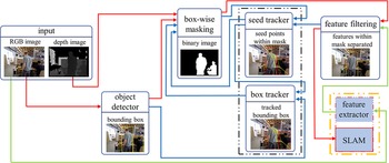
Architecture of the proposed approach. The flow of data through the two main modules, namely masking module and tracking module are indicated by red and blue arrows, respectively. The feature extractor module is a part of the SLAM algorithm – here, the extracted features are not fed directly into SLAM algorithm rather filtered using the mask image. Filtered out features are used as seed points and tracked into the next frame and fed into the masking module to obtain a better masking consistency.

The proposed approach presented in this paper leverages the escalating reliability of semantic detection to retrieve semantic information of the working environment and employs DFS algorithm to obtain masks of semantics belonging to probable dynamic objects using depth images – augmenting the novelty of the work. The resolution of mask image is smaller than the resolutions of the depth and RGB images, where the mask image is scaled down by a scaling factor and the same factor is used to skip pixels in the depth image during traversal such that the computation cost be reduced. In addition, the consistency of object masking is obtained through a tracking module which tracks features belonging to dynamic objects, hence achieving an approach that do not entirely reject the dynamic region but continues to exploit them, adding to the robustness of the algorithm. The proposed approach is also tested over outdoor data, which many of the discussed methods are not tested upon.
3. Framework
This section gives an overview of the proposed approach by discussing in brief the key modules which are incorporated into a SLAM algorithm. The architecture of the proposed approach is shown in Fig. 1. The system takes the
 $i$
th RGB and depth image pair
 $\left( {{\boldsymbol{{I}}_i},\boldsymbol{{D}}_{i}} \right)$
as input. The RGB image
 $\boldsymbol{{I}}_{{i}}$
is fed into the object detection module to obtain bounding boxes
 $B_i^{det} = \left\{ {\boldsymbol{{b}}_{i,\,l}^{det}} \right\}$
of semantics belonging to probably dynamic class. For example, a person in an indoor environment or pedestrian and vehicle on a roadway in an urban environment to mention a few can be considered highly likely non-static. The masking module sorts the bounding boxes
 ${B_i}$
using
 $\boldsymbol{{D}}_{i}$
and employs both
 ${B_i}$
and
 $\boldsymbol{{D}}_{i}$
to generate a scaled-down binary mask image
 $\boldsymbol{{M}}_{i}$
representing the pixel-level dynamic entities. Occasionally, a bounding box which has been detected in the previous frame may not get detected in the current frame and to cope with such undetected objects, seed points are employed to track the boxes. A seed point is a characteristic point within a bounding box being tracked that is additionally given for the generation of mask images accounting for the undetected objects. The mask image
 $\boldsymbol{{M}}_i$
is then used to eliminate point-features being extracted by the SLAM algorithm from being registered for pose estimation and mapping since they represent dynamic objects.
The features within the mask are tracked and used in the following frame to handle the case when an object goes undetected. The tracking module uses the feature points (called seed points)
 ${S_{i,\,l}} = \left\{ {s_{i,\,l}^q} \right\}$
belonging to the mask in the current frame say
 ${f_i}$
and tracks them to the next frame say
 ${f_{i+1}}$
as
 $S_{i,\,l}^{track} = \left\{ {s_{i,\,l}^{q,track}} \right\}$
, where
 $S_{i,\,l}^{track} \subseteq {S_{i,\,l}}$
, such that if either masking module fails to generate adequate mask or the object detection module fails to detect an object, the tracking module attempts to generate new mask or obtain boxes from previously generated mask, respectively, using
 $S_{i,\,l}^{q,track}$
. It is important to note that in the term
 $S_{i,\,l}^{track}$
, the subscript
 $i$
indicates that the seed points are being tracked from the
 $i$
th frame to the
 $i+1$
th frame and
 $l$
indicates the box labels. In the following sections, the modules are discussed in detail.
4. Object Detection
The object detection module takes the RGB image
 ${\boldsymbol{{I}}}_{i}$
as input, detects semantics, classify the semantics based on how likely a semantic belongs to a dynamic object class and outputs a set of bounding boxes, say
 $B_{i,\,l}^{det}$
of detected semantics belonging to dynamic classes. Here, the subscript
 $i$
represents the frame number and
 $l$
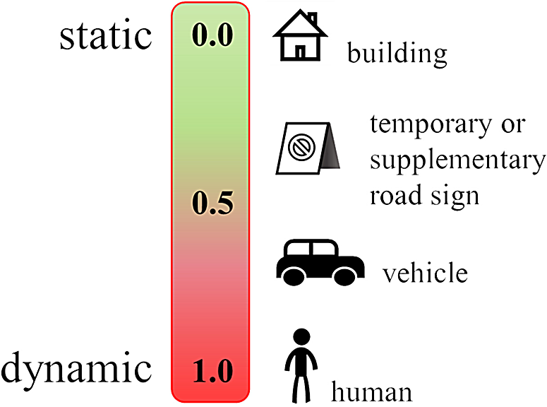
represents the l th box detected. Fig. 2 shows an illustration of classifying semantics based on how likely the semantics are dynamic. The threshold for deciding which semantics belong to a dynamic class can be assigned accordingly. Ample number of DNN based object detection frameworks are accessible that detect objects and returns corresponding bounding boxes [Reference Zhao, Zheng, Xu and Wu38].
Illustration of classifying semantics based on how likely a semantic is static or dynamic using probabilistic approach.

The bounding boxes are generally stored as a
 $1 \times 4$
array or vector which consist of only the minimum and maximum height and width values in the image plane instead of storing all the four corners. For example, a bounding box, say
 $\boldsymbol{{b}}_{i,\,l}^{det} \in B_i^{det}$
, is stored as
 $\boldsymbol{{b}}_{i,\,l}^{det} = \left[ {x_{i,\,l}^{min},y_{i,\,l}^{min},x_{i,\,l}^{max},y_{i,\,l}^{max}} \right]$
, where
 $x_{i,\,l}^{min}$
and
 $x_{i,\,l}^{max}$
are the minimum and maximum corner values of the box along the height of the image and the same for
 $y_{i,\,l}^{min}$
and
 $y_{i,\,l}^{max}$
along the width. This format of storing bounding boxes is a conventional approach of storing bounding boxes by most DNN-based object detectors. The bounding boxes allow the masking to be confined within a box, hence limiting the masking module from brimming the mask beyond the box.
5. Masking and Point Filtering
This module attempts to generate binary mask image
 $\boldsymbol{{M}}_{i}$
using the depth image
 $\boldsymbol{{D}}_{i}$
if the object detection module detects any dynamic object
 $\boldsymbol{{b}}_{i,\,l}^{det}$
or the tracking module tracks a box
 $\boldsymbol{{b}}_{i - 1,l}^{track}$
belonging to dynamic object. The objects considered in the mask image (
 $B_i^{merge}$
) are thus a union of the ones contained in the detected bounding box (
 $B_i^{det}$
) and the tracked bounding box (
 $B_{i - 1}^{track}$
), considering an object only once if it appears in both in
 $B_i^{det}$
and
 $B_{i - 1}^{track}$
. All these will be subsequently tracked. The module sorts the boxes based on their local depth data using
 $\boldsymbol{{D}}_{i}$
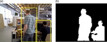
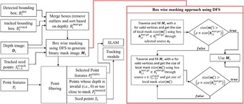
. Fig. 3 shows a generated binary mask image, and the overview of this module is depicted in Fig. 4. One of the main reasons behind why masking is achievable using the depth image for each bounding box is because the foreground in the depth image will typically belong to the semantic being detected.
An illustration of mask image obtained through detected bounding boxes. (a) Bounding boxes of two semantics belonging to highly likely dynamic class (human) being detected (b) Binary mask image experimentally generated using corresponding depth image and bounding boxes.

A schematic representation of the masking module along with the point filtering approach. The box wise masking approach is represented separately in the red box.

The dynamic object is not the complete bounding box, but a masked region of the bounding box represented in the mask image
 $\boldsymbol{{M}}_{i}$
. The generation of the image is done by using a depth-first search (DFS)-based flood-fill like algorithm using the depth image. Leaving a dynamic object is characterized by a sudden change of the depth. The module first generates a lower resolution mask image
 $\boldsymbol{{M}}_{i}$
which is scaled down by a scaling factor, say
 $k$
as:
 \begin{equation}\boldsymbol{{M}}_{i} \leftarrow zeros\left( {\frac{h}{k},\frac{w}{k}} \right)\end{equation}
where the function
 $zeros\left( {} \right)$
generates an image filled with intensity value of
 $0$
, the terms
 $h$
and
 $w$
are the height and width of the depth image
 $\boldsymbol{{D}}_{i}$
(or RGB
 ${\boldsymbol{{I}}_i}$
, given that both RGB and depth images have the same resolution), respectively. Suppose if
 $k\;=\;2$
, then the resolution of
 $\boldsymbol{{M}}_{i}$
will be half the resolution of
 $\boldsymbol{{D}}_{i}$
. The rescaling factor
 $k$
is an essential component in reducing the time required for generating the mask.
Using
 $\boldsymbol{{D}}_{i}$
, the module firstly attempts to fill
 $\boldsymbol{{M}}_{i}$
with a specified intensity value or masking value, say
 $\alpha $
where
 $0 \le \alpha \le 255$
(any valid intensity value greater than zero) as DFS traverses through
 ${\boldsymbol{{D}}_{i,\,l}}$
within each box
 $\boldsymbol{{b}}_{i,\,l}^{merge} \in B_i^{merge}$
. The depth-first search requires a characteristic point to start the flood-fill called as the seed point, say
 $\boldsymbol{{o}}$
representing any point on the dynamic object. If adequate mask is generated for each box
 $\boldsymbol{{b}}_{i,\,l}^{merge} \in B_i^{merge}$
through,
 $\boldsymbol{{o}},\boldsymbol{{M}}_{i}$
is used to filter or rather separate the dynamic and static features. If for any box, the size of the local mask is lesser than a threshold, the module loops through the seed points
 $S_{i - 1,l}^{track}$
being tracked from previous frame, say
 ${f_{i - 1}}$
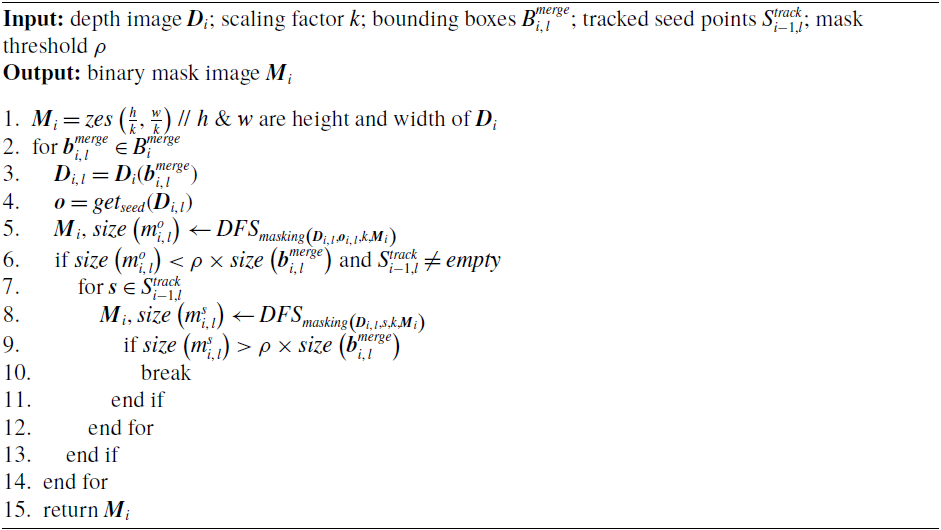
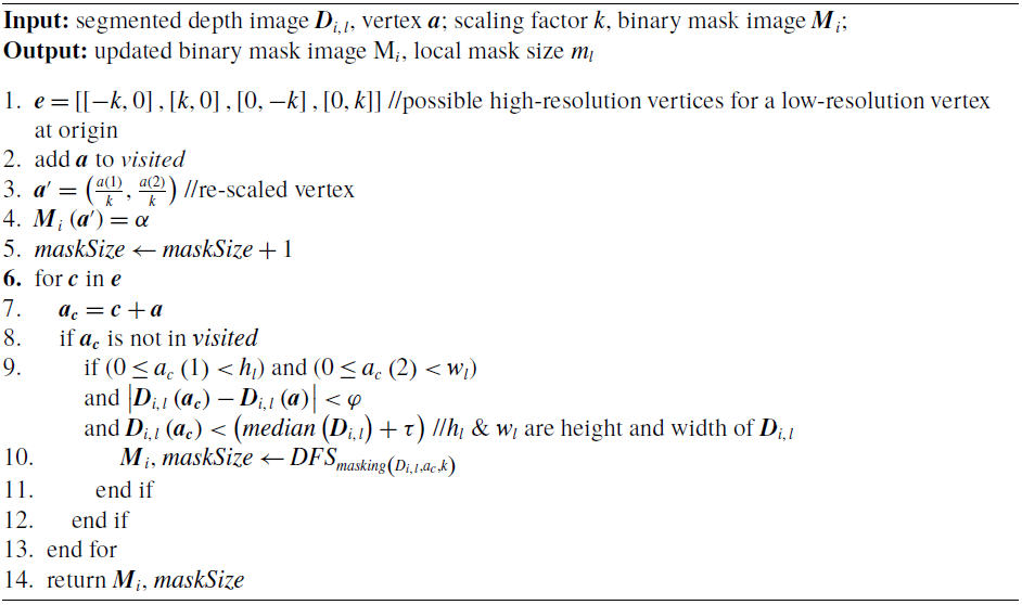
to generate the mask by using the tracked seed points as the source. The pseudocodes of depth masking approach and the DFS method for filling the mask image
 $\boldsymbol{{M}}_{i}$
are presented in Algorithm 1 and Algorithm 2, respectively. The correspondence matching method and the approaches for generating
 $\boldsymbol{{M}}_{i}$
are discussed in detail in the following sub-sections.
5.1 Box merging
This sub-module removes duplicates while taking a union of the detected and tracked boxes and then sorts them based on the depth data. Any tracked box in
 $B_{i - 1}^{track}$
that is detected in the current frame is updated to the new observation, while the ones not detected are retained from the previous. This approach loops through
 $B_{i - 1}^{track}$
and compares the distance between each tracked box, say
 $\boldsymbol{{b}}_{i - 1,l}^{track} \in B_{i - 1}^{track}$
against all the detected boxes
 $B_i^{det}$
. For any box
 $b_{i - 1,l}^{rack} \in B_{i - 1}^{track}$
whose
depth masking

DFS masking

distance is less than a threshold, say
 $\zeta $
against any box in
 $B_i^{det}$
, the box
 $\boldsymbol{{b}}_{i - 1,l}^{track}$
is eliminated else, stored for masking. This can be represented as:
 \begin{equation}remove\left( {\boldsymbol{{b}}_{i - 1,l}^{track}} \right) = \left\{ {\begin{array}{*{20}{l}}{True,if\;{\exists _{{b_{i,\,l}} \in B_{i,\,l}^{det}}}\left| {\boldsymbol{{b}}_{i - 1,l}^{track} - b_{i,\,l}^{det}} \right| < \zeta }\\ {False,otherwise}\end{array}} \right.\end{equation}
Note that the term
 $l$
represents different
 ${l^{th}}$
boxes and does not relate the
 ${l^{th}}$
box of
 $B_i^{det}$
to the
 ${l^{th}}$
box of
 $B_{i - 1}^{track}$
. If Eq. (1) holds
 $True$
for any detected box
 $\boldsymbol{{b}}_{i,\,l}^{det} \in B_i^{det}$
against any
 $\boldsymbol{{b}}_{i - 1,l}^{track} \in B_{i - 1}^{track}$
, the box
 $\boldsymbol{{b}}_{i - 1,l}^{track}$
is eliminated such that the union will accept the updated observation. The non-eliminated boxes in
 $B_{i - 1}^{track}$
and all boxes in
 $B_i^{det}$
are used to generate the mask image. The boxes after the union are given by:
 \begin{equation}B_i^{merge} = B_i^{det} \cup \left\{ {b_{i - 1,l}^{track} \in B_{i - 1}^{track}:\neg remove\left( {\boldsymbol{{b}}_{i - 1,l}^{track}} \right)} \right\}\end{equation}
The boxes from Eq. (3) are then sorted based on the mean of the depth within each box using the depth image
 $\boldsymbol{{D}}_{i}$
. Using each box
 $\boldsymbol{{b}}_{i,\,l}^{merge} \in B_i^{merge}$
, a local or sub-depth image is segmented or sliced, say
 ${\boldsymbol{{D}}_{i,\,l}}$
, and the mean depth of each
 ${\boldsymbol{{D}}_{i,\,l}}$
is computed. The mean depth of all boxes, say
 $\left[ {{\bar{\boldsymbol{{D}}}_{i,1}},{{\bar{\boldsymbol{{D}}}}_{i,2}}, \ldots } \right],$
is then sorted in a descending order based on the depth value and the order of the sorted depth means is reflected on each
 $\boldsymbol{{b}}_{i,\,l}^{merge} \in B_i^{merge}$
.
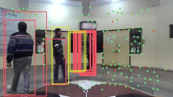
The correspondence matched box removal is performed to remove redundancies in boxes. If outliers are not removed, the number of boxes can interpolate and increase over time, generating unnecessary boxes and if not controlled, boxes can be generated unlimitedly. An illustration of this is shown in Fig. 5 – experimentally generated. On the other hand, the boxes are sorted to assign each seed point to the correct box it belongs to. This is further discussed in section 5.5.
Illustration of box tracking error (experimentally generated) interpolating over time due to uncontrolled box tracking. This occurs when the tracked box which is too close, which is also corresponding to a newly detected box is not removed. Here, yellow box and red box represent detected and tracked boxes, respectively.

5.2 Generating mask from a selected source
This approach is the default method for generating the mask – since seed points are obtained only from a previously generated mask. For each box
 $\boldsymbol{{b}}_{i,\,l}^{merge} \in B_i^{merge}$
, the source
 $o$
is selected by first dividing or slicing the depth image
 $\boldsymbol{{D}}_{i}$
within
 ${\boldsymbol{{b}}_{i,\,l}}$
into four grids, say
 $\boldsymbol{{D}}_{i,\,l}^g$
where
 $g\;=\;1,2,3,4 $
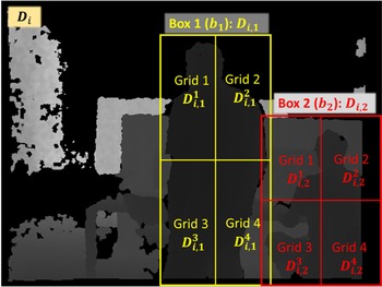
and the mean or average depth of each grid is computed – an illustration of slicing boxes into four grids is shown in Fig. 6. The size of
 $g$
or rather the number of grids is flexible and can be set to any valid value. After which, the index of the pixel whose depth is closest to the minimum of the four means is selected as the source for each box in
 $B_i^{merge}$
:
 \begin{equation}\boldsymbol{{o}} = arg\;mi{n_o}\left| {\mathop {\min }\limits_g \left( {\overline {\boldsymbol{{D}}_{i,\,l}^g} } \right) - {\boldsymbol{{D}}_{i,\,l}}\left( o \right)} \right|\end{equation}
Illustration of slicing boxes into grids. Here, the term
 ${\boldsymbol{{D}}_{i,1}}$
corresponds to the depth image obtained from bounding box
 ${\boldsymbol{{b}}_1}$
belonging to set of detected boxes
 ${B_{i,j}}$
and the term
 $i$
represents the frame number.

Here, the overall equation returns the image coordinate or the index of the pixel with a depth which is closest to the minimum mean depth of the grids; the function
 ${\boldsymbol{{D}}_{i,\,l}}\left( \boldsymbol{{o}} \right)$
gives the depth of a point
 $o$
using the depth image the term;
 $g$
represents the grids; the bar symbol is used to denote the mean depth of the sliced depth image grid. For four grids,
 $min\left( {\boldsymbol{{D}}_{i,\,l}^g} \right)$
bears:
 \begin{equation}min\left( \boldsymbol{{D}}_{i,\,l}^{g} \right) = \min \left( \bar{\boldsymbol{{D}}}_{i,\,l}^1,\bar{\boldsymbol{{D}}}_{i,\,l}^2,\bar{\boldsymbol{{D}}}_{i,\,l}^3,\bar{\boldsymbol{{D}}}_{i,\,l}^4 \right)\end{equation}
The reason behind slicing the sub-depth images
 ${\boldsymbol{{D}}_{i,\,l}}$
into grids is to assist the module in obtaining a more consistent masking. Consider the grids in Box 2 as shown in Fig. 6. In grid 1 of Box 2, the number of pixels belonging to the foreground (semantic class: human) is considerably lesser compared to the background pixels while in grid 4, most of the pixels belongs to the foreground and providing more consistent depth within the foreground. Regardless, depending on the type of data used, the approach of slicing
 ${\boldsymbol{{D}}_{i,\,l}}$
can be dropped if needed, wherein the index of the pixel with the depth closest to the mean of the depth in
 ${\boldsymbol{{D}}_{i,\,l}}$
can be used as the source, that is:
 \begin{equation}\boldsymbol{{o}} = arg\;mi{n_o}\left| {\overline {{\boldsymbol{{D}}_{i,\,l}}} - {\boldsymbol{{D}}_{i,\,l}}\left( \boldsymbol{{o}} \right)} \right|\end{equation}
Here, the equation returns the index of the any pixel within
 ${\boldsymbol{{D}}_{i,\,l}}$
whose depth is closest to the mean depth. Using the obtained source
 $\boldsymbol{{o}}$
for the th box, DFS is employed to traverse across
 ${\boldsymbol{{D}}_{i,\,l}}$
to fill
 $\boldsymbol{{M}}_{i}$
with
 $\alpha $
. The scaling factor
 $k$
is used to skip pixels during traversal to reduce the time required to generate masks. The approach of depth image traversal is described in section 5.4.
For each box, a count for the number of vertices or pixels being visited is maintained. In other terms, the size of each local mask, say
 $size\left( {\boldsymbol{{m}}_{i,\,l}^o} \right),$
is recorded as DFS traverses across each
 ${\boldsymbol{{D}}_{i,\,l}}$
, where the function
 $size\left( {} \right)$
returns the count of all visited vertices. The term
 $o$
in
 $\boldsymbol{{m}}_{i,\,l}^o$
represents the source being selected from the mentioned approach. Using
 $size\left( {\boldsymbol{{m}}_{i,\,l}^o} \right)$
, the decision on whether the mask needs to be re-generated using seed points is made which is assisted by a minimum mask size threshold
 $\rho $
.
 \begin{equation}\gamma _{i,\,l}^o = \left\{ {\begin{array}{*{20}{l}}{True,if\;size\left( {\boldsymbol{{m}}_{i,\,l}^o} \right)}\quad { > \rho \times size\left( {\boldsymbol{{b}}_{i,\,l}^{merge}} \right)}\\[5pt] {False,otherwise}\end{array}} \right.\end{equation}
Here,
 $\gamma _{i,\,l}^o$
stores the binary value for deciding whether the mask should be regenerated for the
 ${l^{th}}$
box;
 $\rho $
is the percentile threshold, where
 $0 \le \rho \le 1$
;
 $size\left( {} \right)$
returns the number of valid pixels – for
 $\boldsymbol{{m}}_{i,\,l}^o$
, it returns the number of visited pixels, whereas for
 $b_{i,\,l}^{merge}$
, it returns the number of pixels within the box
 $\boldsymbol{{b}}_{i,\,l}^{merge}$
. In Eq. (6),
 $\gamma _{i,\,l}^o$
holds
 $True$
for the
 ${l^{th}}$
box if the size of local mask
 $\boldsymbol{{m}}_{i,\,l}^{}$
is greater than a certain percentage (assigned to
 $\rho )$
of the total number of pixels within
 ${\boldsymbol{{D}}_{i,\,l}}$
or here, simply the size of box
 $\boldsymbol{{b}}_{i,\,l}^{merge} \in B_{i,\,l}^{merge}$
. If
 $\gamma _{i,\,l}^{}$
is
 $True$
, the mask generated using
 $\boldsymbol{{b}}_{i,\,l}^{merge}$
is accepted else, an attempt to re-generate the mask is made by using the tracked seed points
 $S_{i - 1,l}^{ack}$
, which is discussed in the next sub-section.
5.3 Generating mask using seed points
In Eq. (7), if
 $\gamma _{i,\,l}^o$
holds
 $False$
, this sub-module loops through the tracked seed points
 $S_{i - 1,l}^{track}$
, using the index of each seed point as the source, over which DFS traverses through the corresponding
 ${\boldsymbol{{D}}_{i,\,l}}$
to fill
 $\boldsymbol{{M}}_{i}$
with
 $\alpha $
for valid pixels (the approach is described in section 5.4). The approach of selecting the seed points is discussed in section 5.5. The loop is terminated at any timestamp if the following equation holds
 $True$
:
 \begin{equation}\gamma _{i,\,l}^s = \left\{ {\begin{array}{*{20}{l}}{True,if\; size\left( {\boldsymbol{{m}}_{i,\,l}^s} \right)}\quad { > \rho \times size\left( {\boldsymbol{{b}}_{i,\,l}^{merge}} \right)}\\[5pt] {False,otherwise}\end{array}} \right.\end{equation}
Here, the term
 $s$
corresponds to a seed point in
 $S_{i - 1,l}^{track}$
, that is
 $s \in S_{i - 1,l}^{track},$
wherein the loop iterates through
 $s$
points. The same check is performed as described using Eq. (7) and if
 $\gamma _{i,\,l}^s$
in Eq. (8) is
 $True$
for any
 $s$
, the loop is terminated. If for all
 $s \in S_{i - 1,l}^{track}$
,
 $\gamma _{i,\,l}^s$
holds
 $False$
,
 $\boldsymbol{{M}}_{i}$
is filled with
 $\alpha $
for the box
 ${\boldsymbol{{b}}_l}$
entirely.
5.4. DFS Based masking
The depth-first search algorithm is employed to fill
 $\boldsymbol{{M}}_{i}$
with
 $\alpha $
where
 $0 < \alpha \;<\;255$
as it traverses over each
 ${\boldsymbol{{D}}_{i,\,l}}$
to generate the binary mask image. Here,
 ${\boldsymbol{{D}}_{i,\,l}}$
is obtained by segmenting the region in
 $\boldsymbol{{D}}_{i}$
belonging to the box
 $\boldsymbol{{b}}_{i,\,l}^{merge} \in B_i^{merge},$
and it is used as the graph for DFS to traverse. The scaling factor
 $k$
is employed to skip pixels in
 ${\boldsymbol{{D}}_{i,\,l}}$
by a factor of
 $k$
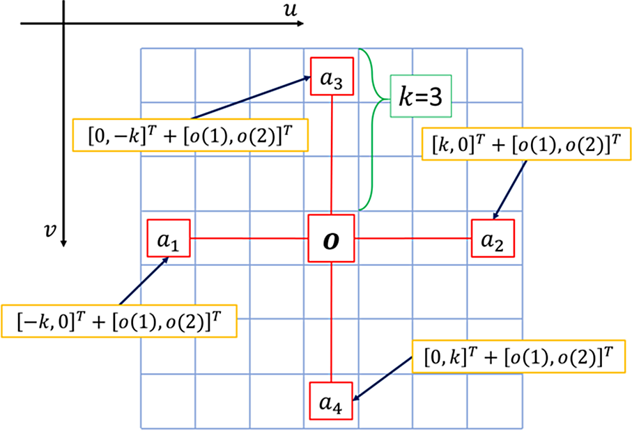
such that the traversal time be reduced. An illustration of skipping pixels is shown in Fig. 7.
An illustration of skipping pixels (vertex) by a scaling factor
 $k$
. Here,
 $o$
is the source, while
 ${\boldsymbol{{a}}_1}$
,
 ${\boldsymbol{{a}}_2}$
,
 ${\boldsymbol{{a}}_3}$
and
 ${\boldsymbol{{a}}_4}$
are the possible vertices that DFS can visit for
 $k\;=\;3$
from the vertex
 $\boldsymbol{{o}}$
.

Due to a reduction of resolution, a vertex known to be at origin in the lower-resolution map can be at either of the points in the higher resolution bounded by the points
 $e = \left[ {{\boldsymbol{{e}}_1},{\boldsymbol{{e}}_2},{\boldsymbol{{e}}_3},{\boldsymbol{{e}}_4}} \right]$
where
 ${\boldsymbol{{e}}_1} = {\left[ { - k,0} \right]^T}$
,
 ${\boldsymbol{{e}}_2} = {\left[ {k,0} \right]^T}$
,
 ${\boldsymbol{{e}}_3} = {\left[ {0, - k} \right]^T}$
and
 ${\boldsymbol{{e}}_4} = {\left[ {0,k} \right]^T}$
and k is the reduction factor of resolution. So, for a current vertex, say, the neighbouring vertices to be visited, say
 ${\boldsymbol{{a}}_1}$
,
 ${\boldsymbol{{a}}_2}$
,
 ${\boldsymbol{{a}}_3}$
and
 ${\boldsymbol{{a}}_4}$
are iteratively obtained by adding
 $\boldsymbol{{e}}$
as follows:
 \begin{equation}{\boldsymbol{{a}}_1} = {\boldsymbol{{e}}_1} + \boldsymbol{{a}} = {\left[ { - k,0} \right]^T} + {\left[ {a\left( 1 \right),a\left( 2 \right)} \right]^T}\end{equation}
 \begin{equation}{\boldsymbol{{a}}_2} = {\boldsymbol{{e}}_2} + \boldsymbol{{a}} = {\left[ {k,0} \right]^T} + {\left[ {a\left( 1 \right),a\left( 2 \right)} \right]^T}\end{equation}
 \begin{equation}{\boldsymbol{{a}}_3} = {\boldsymbol{{e}}_3} + \boldsymbol{{a}} = {\left[ {0, - k} \right]^T} + {\left[ {a\left( 1 \right),a\left( 2 \right)} \right]^T}\end{equation}
 \begin{equation}{\boldsymbol{{a}}_4} = {\boldsymbol{{e}}_4} + \boldsymbol{{a}} = {\left[ {0,k} \right]^T} + {\left[ {a\left( 1 \right),a\left( 2 \right)} \right]^T}\end{equation}
In Eqs. (9)–(12), the terms
 $a\left( 1 \right)$
and
 $a\left( 2 \right)$
are the image coordinates of vertex
 $\boldsymbol{{a}}$
. In Fig. 7, the current vertex is the source
 $\boldsymbol{{o}}$
, while the neighbouring vertices
 ${\boldsymbol{{a}}_1}$
,
 ${\boldsymbol{{a}}_2}$
,
 ${\boldsymbol{{a}}_3}$
and
 ${\boldsymbol{{a}}_4}$
to be visited are iteratively obtained by adding
 $\boldsymbol{{e}}$
whose
 $k\;=\;3$
.
In addition to the validation check performed by DFS – where the algorithm traverses to a neighbouring vertex only if the vertex is not being visited before – three extended validations are performed before adding any neighbouring vertex for traversal:
-
1. Validation using box limits: A neighbouring pixel is validated by checking against the box limits, that is, if for any neighbouring vertex
 ${\boldsymbol{{a}}_c} = {\left[ {{a_c}\left( 1 \right),{a_c}\left( 2 \right)} \right]^T}$
, where
$c\;=\;1,2,3,4$
, if either
${\boldsymbol{{a}}_c}\left( 1 \right)$
or
${\boldsymbol{{a}}_c}\left( 2 \right)$
exceeds any of limits in referencing box
${\boldsymbol{{b}}_{i,\,l}} = \left[ {{x_{i,l,min}},{y_{i,l,min}},{x_{i,l,max}},{y_{i,l,max}}} \right]$
, the vertex
${a_c}$
is set as an invalid vertex.
-
2. Validation using differential depth difference: Traversal from a foreground dynamic object to a background in the depth image is characterized by a sudden change in the depth. The depth distance, say
$\delta \left( {{\boldsymbol{{a}}_c},\boldsymbol{{a}}} \right)$
between the current vertex, say
$\boldsymbol{{a}}$
and its neighbouring vertex, say
${a_c}$
which is yet to be visited, is checked. If
$\delta \left( {{\boldsymbol{{a}}_c},\boldsymbol{{a}}} \right)$
is larger than a threshold, say
$\varphi $
, the vertex
${\boldsymbol{{a}}_c}$
is set as an invalid vertex. This can be represented as:


 \begin{equation}valid\left( {{\boldsymbol{{a}}_c}} \right) = \left\{ {\begin{array}{*{20}{l}}{True,\quad if\delta \left( {{\boldsymbol{{a}}_c},\boldsymbol{{a}}} \right) < \varphi }\\[5pt] {False, \qquad otherwise}\end{array}} \right.\end{equation}
where the depth distance
 $\delta \left( {{\boldsymbol{{a}}_c},\boldsymbol{{a}}} \right)$
is defined as:
 \begin{equation}\delta \left( {{\boldsymbol{{a}}_c},\boldsymbol{{a}}} \right) = |{\boldsymbol{{D}}_{i,\,l}}\left( {{\boldsymbol{{a}}_c}} \right) - {\boldsymbol{{D}}_{i,\,l}}\left( \boldsymbol{{a}} \right)|\end{equation}
Here, in Eq. (14),
 ${\boldsymbol{{D}}_{i,\,l}}\left( \boldsymbol{{a}} \right)$
is the depth value at vertex or pixel
 $\boldsymbol{{a}}$
and similarly for
 ${\boldsymbol{{D}}_{i,\,l}}\left( {{\boldsymbol{{a}}_c}} \right)$
. This validation limits DFS from traversing to a neighbouring vertex whose depth difference with the current vertex is larger than a threshold, avoiding sudden change in depth which limits the traversal in the foreground.
Validation using depth tolerance: Normally, the foreground dynamic objects have a small variation in their depth values. A depth tolerance, say
 $\tau ,$
is defined such that if the depth value of a neighbouring pixel, say
 ${\boldsymbol{{a}}_c}$
which is yet to be visited has a depth value larger than sum of
 $\tau $
and median depth of
 ${\boldsymbol{{D}}_{i,\,l}}$
, the vertex
 ${\boldsymbol{{a}}_c}$
is considered invalid. This can be represented as:
 \begin{equation}valid\left( {{\boldsymbol{{a}}_c}} \right) = \left\{ {\begin{array}{*{20}{l}}{True,\quad if\ {\boldsymbol{{D}}_{i,\,l}}\left( {{\boldsymbol{{a}}_c}} \right) < } \quad {median\left( {{\boldsymbol{{D}}_{i,\,l}}} \right) + \tau }\\[5pt] {False, \qquad otherwise}\end{array}} \right.\end{equation}
Here, the function
 $median\left( {{\boldsymbol{{D}}_{i,\,l}}} \right)$
returns the median depth value of the segmented depth image
 ${\boldsymbol{{D}}_{i,\,l}}$
. This validation limits DFS from traversing too far from the median depth. The threshold
 $\tau $
can be obtained based on the type of semantic being dealt with. For example, if the semantic is of human class,
 $\tau $
can range from say
 $0.5\;meters$
to
 $1.5\;meters$
.
In all the three-validation courses, if one of them holds
 $False$
– that is, if the vertex is invalid – the neighbouring vertex
 ${\boldsymbol{{a}}}_{c}$
is eliminated from the graph. The validations using the depth values enables the masking module to segment out the foreground from the background and hence generating a mask of the foreground.
Since the resolution of
 $_i$
is scaled down by the same scaling factor
 $k$
(as shown in Eq. (1)) – which is added to skip pixels while traversing (Eqs. (9)–(12)) – every valid vertex or pixel location being visited can simply be divided by
 $k$
to obtain the corresponding pixel location of
 $\boldsymbol{{M}}_{i}$
, which is to be filled or rather assigned with the masking value
 $\alpha $
. For example, if a current vertex being visited, say
 $\boldsymbol{{a}}$
is valid,
 $\boldsymbol{{M}}_{i}$
can be replaced by
 $\alpha $
using:
 \begin{equation}\boldsymbol{{M}}_{i}\left( {\frac{{a\left( 1 \right)}}{k},\frac{{a\left( 2 \right)}}{k}} \right) = \alpha \end{equation}
The mask image
 $\boldsymbol{{M}}_{i}$
is simultaneously filled by
 $\alpha $
for every valid vertex as DFS traverses across each
 ${\boldsymbol{{D}}_{i,\,l}}$
. This simultaneous approach of filling eliminates the need of refilling
 $_{}$
after DFS traversal.
5.5 Point filtering or point classification
This module separates extracted features, say
 ${P_i}$
into three classes: features to be employed for SLAM
 $P_i^{static}$
; seed points
 ${S_i} = \left\{ {{S_{i,\,l}}} \right\}$
; and invalid points
 $P_i^{invlid}$
– points with either invalid depth or which are too close to the mask. Hence,
 ${P_i}$
can be represented as
 ${P_i} = P_i^{static} \cup {S_i} \cup P_i^{invalid}$
. The module loops through all
 $n$
features and checks to which class a feature belongs and stores or eliminate them accordingly. The approach of filtering or classifying features is discussed below:
5.5.1 Eliminating invalid features
Firstly, for any point feature
 ${\boldsymbol{{p}}_i} \in {P_i}$
, if the depth is invalid, that is
 $\boldsymbol{{D}}_{i}\left( {{\boldsymbol{{p}}_i}} \right)\;=\;0$
, the point
 ${\boldsymbol{{p}}}_{i}$
is eliminated. Secondly, if a feature has a valid depth but is too close to the mask, the feature is set as an invalid feature. This is performed to increase the confidence of selecting static features for performing SLAM – features too close to the edge of the mask are more vulnerable in being non-static. In this elimination method, an inflate factor
 $\sigma $
is defined wherein, for a point
 ${\boldsymbol{{p}}_i}$
which is then rescaled as
 ${\boldsymbol{{p}}'_{\!\!i}} = \dfrac{{{p_i}}}{k}$
,
 $\sigma $
is used to define a squared-window, say
 $W\!\left(\,{\boldsymbol{{p}}'_{\!\!i}} \right)$
around the candidate point
 ${\boldsymbol{{p}}'_{\!\!i}}$
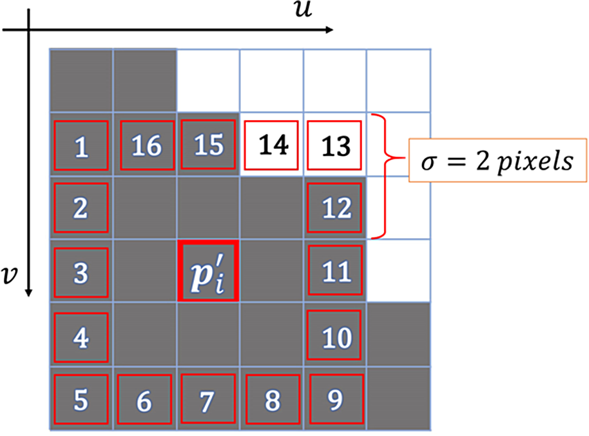
. An illustration of generating
 $W\!\left(\,{\boldsymbol{{p}}'_{\!\!i}} \right)$
around a point
 ${\boldsymbol{{p}}'_{\!\!i}}$
with
 $\sigma \;=\;2$
is shown in Fig. 8. The window
 $W\!\left(\,{\boldsymbol{{p}}'_{\!\!i}} \right)$
can be defined as:
 \begin{equation}W\!\left(\,{\boldsymbol{{p}}'_{\!\!i}} \right) = \left[ {{x_{{\rm{min}}}}\left(\,{\boldsymbol{{p}}'_{\!\!i}} \right),{y_{{\rm{min}}}}\left(\,{\boldsymbol{{p}}'_{\!\!i}} \right),{x_{{\rm{max}}}}\left(\,{\boldsymbol{{p}}'_{\!\!i}} \right),{y_{{\rm{max}}}}\left( {p'_{\!\!i}} \right)} \right]\end{equation}
Illustration of checking a feature being close to the mask. Here, the white pixels belong to the mask, while the grey pixels belong to static background;
 ${\boldsymbol{{p}}'_{\!\!i}}$
is the feature being validated, while pixels numbered 1 to 16 are the neighbouring pixels to be checked – the neighbouring pixels obtained by using a window around
 ${\boldsymbol{{p}}'_{\!\!i}}$
whose inflate factor
 $\sigma $
is 2 pixels.

Or,
 \begin{equation}W\!\left(\,{\boldsymbol{{p}}'_{\!\!i}} \right) = \left[ {{\boldsymbol{{p}}'_{\!\!i}}\left( 1 \right) - \sigma ,{\boldsymbol{{p}}'_{\!\!i}}\left( 2 \right) - \sigma ,{\boldsymbol{{p}}'_{\!\!i}}\left( 1 \right) + \sigma ,{\boldsymbol{{p}}'_{\!\!i}}\left( 2 \right) + \sigma } \right]\end{equation}
Feature close to mask

where the terms
 ${\boldsymbol{{p}}'_{\!\!i}}\left( 1 \right)$
and
 ${\boldsymbol{{p}}'_{\!\!i}}\left( 2 \right)$
are the pixel coordinates of the point
 ${\boldsymbol{{p}}'_{\!\!i}}$
. Here, it is imperative that
 $W\!\left(\,{\boldsymbol{{p}}'_{\!\!i}} \right)$
is within the image height and width limits. If the border of
 $W\!\left(\,{\boldsymbol{{p}}'_{\!\!i}} \right)$
exceeds image size limits, the border pixels of the image itself could be used. This filtering scans the pixels, say
 $w$
along the boundary of
 $W\!\left(\,{\boldsymbol{{p}}'_{\!\!i}} \right)$
for any intensity equal to masking value
 $\alpha $
. The border pixels are first scanned across either
 $u$
-
 $axis$
or
 $v$
-
 $axis$
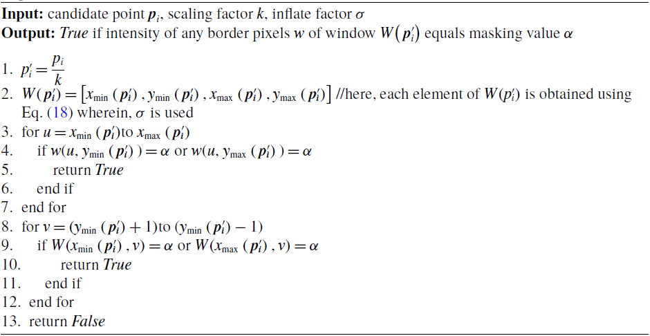
along both minimum and maximum limits, followed by scanning along the other axis while making sure that one pixel is validated not more than once. The pseudocode of this filtering approach is shown in Algorithm 3. The algorithm returns
 $True$
if the conditions given in lines 4 and 9 of Algorithm 3 are met. At any point during the scan if any border pixel, say
 $w = \alpha $
,
 ${\boldsymbol{{p}}_i}$
is eliminated. In Fig. 8,
 ${\boldsymbol{{p}}'_{\!\!i}}$
is to be eliminated since pixel number 13 and 14 are within the mask. Depending on the value assigned to
 $\sigma $
, the number of pixels to scan increases or decreases. The time required to check all the pixels along the border of
 $W\!\left(\,{\boldsymbol{{p}}'_{\!\!i}} \right)$
is proportional to the inflate factor
 $\sigma $
. The invalid points are thus
 $P_i^{invalid} = \left\{ {{p_i} \in {P_i}\;:\;\boldsymbol{{D}}_{i}\left( {{\boldsymbol{{p}}_i}} \right)\;=\;0 \vee \frac{{{p_i}}}{k} \in W\!\left( {\frac{{{p_i}}}{k}} \right)} \right\}$
, where for complexity reasons the interior points are approximated by just the boundary.
5.1.1 Separating seed points from extracted features
The extracted features
 ${P_i}$
to be employed for implementing SLAM are filtered using
 $\boldsymbol{{M}}_{i}$
as well. Each feature location being extracted is divided by
 $k$
and compared against the intensity of
 $\boldsymbol{{M}}_{i}$
at the obtained location. If the intensity for a re-scaled feature location in is equal to
 $\alpha $
, the feature is stored as a seed point else, the feature is stored for performing SLAM. In simple terms, features (which are re-scaled) belonging to the mask are used as seed points, while the other valid features are used for SLAM. For a feature say
 ${\boldsymbol{{p}}_i} \in {P_i}$
, the filtering can be performed as:
 \begin{equation}seedPoint\left( {{\boldsymbol{{p}}_i}} \right) = \left\{ {\begin{array}{*{20}{l}}{True,\quad if\boldsymbol{{M}}_{i}\left( {\frac{{{\boldsymbol{{p}}_i}\left( 1 \right)}}{k},\frac{{{\boldsymbol{{p}}_i}\left( 2 \right)}}{k}} \right) = \alpha }\\[5pt] {False,\quad otherwise}\end{array}} \right.\end{equation}
If Eq. (19) holds
 $False$
, the feature
 ${\boldsymbol{{p}}_i}$
is stored and employed in performing SLAM, otherwise it is stored as a seed point. The seed points represent dynamic objects and are conventionally filtered out. Here we store them separately for the generation of the dynamic masked image, should it be impossible by the other points. The seed points are stored in a box wise manner, say
 ${S_{i,\,l}}$
where
 $l$
is the box, or
 $\boldsymbol{{b}}_{i,\,l}^{merge} \in B_i^{merge}$
so that they could be tracked separately by the tracking module, especially for tracking boxes – the tracking module is discussed in section 6. The seed points are thus given by
 ${S_i} = { \cup _l}{S_{i,\,l}} = { \cup _l}\left\{ {{p_i} \in P:seedPoint\left( {{\boldsymbol{{p}}_i}} \right)} \right\}.$
There can also be cases where the boxes overlap, which can result in overlapping masks and this could further result in assigning the seed points to a wrong box. This is attended to by sorting the boxes in descending order – as discussed in section 5.1. As the boxes are in descending order based on the depth, the seed points belonging to an intersecting mask are eventually assigned to the foreground objects or rather boxes. Suppose boxes
 ${\boldsymbol{{b}}_{i,1}}$
and
 ${\boldsymbol{{b}}_{i,2}}$
have overlapping masks, whose mean depths are
 $\bar{\boldsymbol{{D}}}_{i,1}$
and
 $\bar{\boldsymbol{{D}}}_{i,2}$
, respectively. Suppose
 $\bar{\boldsymbol{{D}}}_{i,1} < \bar{\boldsymbol{{D}}}_{i,2}$
that is,
 $\bar{\boldsymbol{{D}}}_{i,1}$
is in front of
 $\bar{\boldsymbol{{D}}}_{i,2}$
. The order after sorting would be
 $[\bar{\boldsymbol{{D}}}_{i,2},\bar{\boldsymbol{{D}}}_{i,1}]$
. If there are seed points belonging to the intersecting mask, the points would be first assigned to
 ${\boldsymbol{{b}}_{i,2}}$
, followed by
 ${\boldsymbol{{b}}_{i,1}}$
and as a result, the seed points would be tracked with respect to the intended box.
The features used for SLAM are thus
 $P_i^{static} = {P_i}\backslash \left( {{S_i} \cup P_i^{invalid}} \right)$
. Say, there are
 $size\left( {{S_{}}} \right)$
seed points and
 $size\left( {P_i^{invalid}} \right)$
invalid points, an amount of
 $\left( {size\left( {{P_i}} \right) - \left( {size\left( {{S_i}} \right) + size\left( {P_i^{invalid}} \right)} \right)} \right)$
points are used for SLAM. In summary, point filtering module first checks if a point has an invalid depth and then separates valid points into either seed points, points close to mask (which are also considered invalid) or points to be used for SLAM.
6. Tracking Module
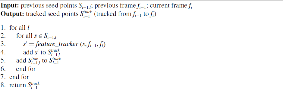
The tracking module tracks the seed points to assist the masking module for regenerating masks and in addition track the bounding boxes as well. The approach to tracking the seed points is not confined to a particular tracking method – Kanade-Lucas-Tomasi (KLT) feature tracker [Reference Lucas and Kanade39, Reference Shi and Tomasi40], Kalman filter, particle filter and feature matching method, to mention a few, are some commonly used point-feature tracking methods.
Box wise feature tracking

Box tracker

The seed points
 ${S_{i - 1,l}}$
are tracked in a box wise manner from previous frame, say
 ${f_{i - 1}}$
to the current frame, say
 ${f_i}$
to obtain
 $S_{i - 1,l}^{track}$
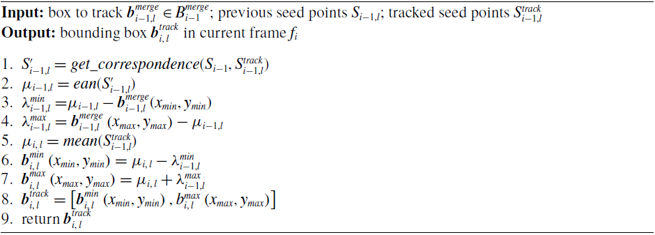
seed points. A brief overview on the box wise seed point tracking is shown in Algorithm 4. The box wise seed point tracking is essential as both mask regeneration and box tracking are performed box wise. For regenerating a mask, the algorithm firstly loops over the boxes
 $B_{i,\,l}^{merge}$
(line 2 of Algorithm 1) and the tracked seed points
 $S_{i - 1,l}^{track}$
belonging to reference box
 $\boldsymbol{{b}}_{i,\,l}^{merge}$
are loop over, using them as the source for DFS traversal (line 7 of Algorithm 1). While for tracking the bounding boxes, the spatial-correlation information between the seed points
 ${S_{i - 1,l}}$
and
 $S_{i - 1,l}^{track}$
is considered to obtain a box. Note that
 ${S_{i - 1,l}}$
are seed points belonging to and
 $S_{i - 1,l}^{track}$
are the tracked seed points being tracked from
 ${f_{i - 1}}$
to
 ${f_i}$
.
In case of tracking boxes, though there is the option to track the corners of a box, the reliability – consistency and accuracy – of tracking them is slim. Features belonging to strong corners are more reliable for tracking and since seed points are basically strong corners, hence they can deliver a more consistent correlation. This module keeps a check on the number of boxes in previous frame
 ${f_{i - 1}}$
, say
 $size\left( {B_{i - 1}^{merge}} \right)$
and if the number of detected boxes
 $B_i^{det}$
reduces in the current frame
 ${f_i}$
, that is
 $size\left( {B_i^{det}} \right) < size\left( {B_{i - 1}^{merge}} \right)$
, it finds and then attempts to generate or track those boxes in which are not detected in
 ${f_i}$
using the seed points
 ${S_{i - 1,l}}$
and tracked seed points
 $S_{i - 1,l}^{track}$
. The pseudocode for obtaining the tracked box is given in Algorithm 5.
For a box to be tracked, say
 $\boldsymbol{{b}}_{i - 1,l}^{merge}$
, the module finds the seed points in
 ${S_{i - 1,l}}$
corresponding to
 $S_{i - 1,l}^{track}$
and computes a spatial correlation between corresponding points, say
 $S_{i - 1,l}^{\prime}$
to define the box in the current frame
 ${f_i}$
. The approach to obtaining corresponding seed points is not confined to a particular method and depends on the type of tracking method used. It is evident that all tracked seed points
 $S_{i - 1,l}^{track}$
will have a corresponding point in
 ${S_{i - 1,l}}$
since
 $S_{i - 1,l}^{track}$
are tracked from
 ${S_{i - 1,l}}$
. Here, an option is to keep track of the indices of points in
 $S_{i - 1,l}^{track}$
successfully tracked to
 ${f_i}$
. After obtaining the corresponding seed points
 $S_{i - 1,l}^{\prime}$
, the mean of all points in
 $S_{i,\,l}^{\prime}$
, say
 ${\mu _{i - 1,l}}$
is computed. Using the mean point
 ${\mu _{i - 1,l}}$
, two lines, say
 $\lambda _{i - 1,l}^{min}$
and
 $\lambda _{i - 1,l}^{max}$
connecting the two corners, say
 $\boldsymbol{{b}}_{i - 1,l}^{min}$
and
 $\boldsymbol{{b}}_{i - 1,l}^{max}$
of the box
 ${\boldsymbol{{b}}_l}$
(referred to the format specified in section 4) is obtained as:
 \begin{equation}\lambda _{i - 1,l}^{min} = \mu _{i - 1,l}^{min} - \boldsymbol{{b}}_{i - 1,l}^{min}\end{equation}
 \begin{equation}\lambda _{i - 1,l}^{max} = \boldsymbol{{b}}_{i - 1,l}^{max} - \mu _{i - 1,l}^{max}\end{equation}
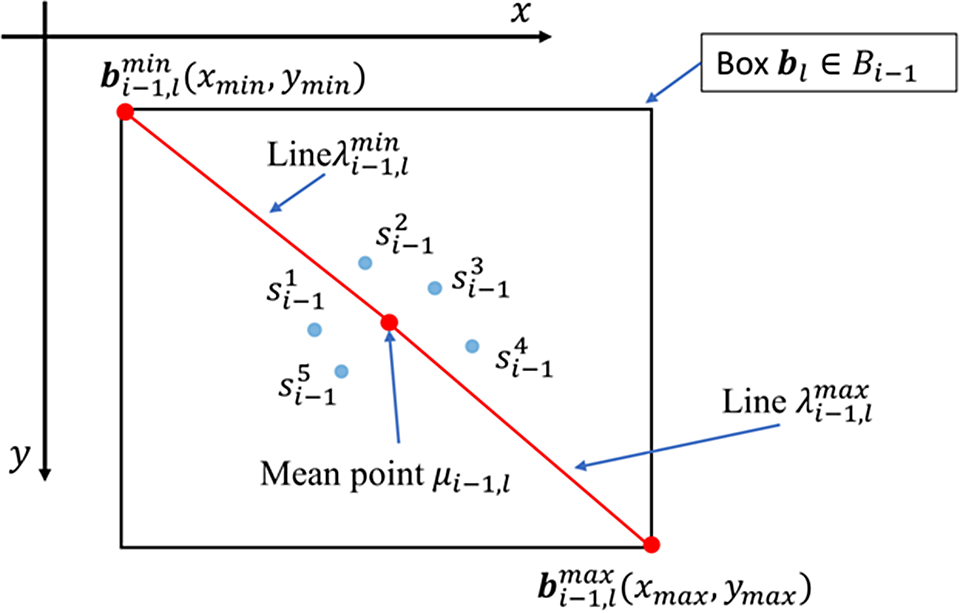
An illustration of obtaining the lines is shown in Fig. 9. After retrieving
 $\lambda _{i - 1,l}^{min}$
and
 $\lambda _{i - 1,l}^{max}$
, the mean point, say
 ${\mu _{i,\,l}}$
for the tracked seed points
 $S_{i - 1,l}^{track}$
in
 ${f_i}$
is computed as well. The lines
 $\lambda _{i - 1,l}^{min}$
and
 $\lambda _{i - 1,l}^{max}$
are then employed to obtain the corner points
 $\boldsymbol{{b}}_{i,\,l}^{min}$
and
 $\boldsymbol{{b}}_{i,\,l}^{max}$
of the new or rather tracked box in the current frame
 $i$
as:
 \begin{equation}\boldsymbol{{b}}_{i,\,l}^{min} = {\mu _{i,\,l}} - \lambda _{i - 1,l}^{min}\end{equation}
 \begin{equation}\boldsymbol{{b}}_{i,\,l}^{max} = {\mu _{i,\,l}} + \lambda _{i - 1,l}^{min}\end{equation}
Illustration of lines
 $\lambda _{i - 1,l}^{min}$
and
 $\lambda _{i - 1,l}^{max}$
connecting the mean point
 ${\mu _{i - 1,l}}$
to the two corners
 $\boldsymbol{{b}}_{i - 1,l}^{min}$
and
 $\boldsymbol{{b}}_{i - 1,l}^{max}$
of a box
 ${\boldsymbol{{b}}_l}$
. The points
 $s_{i - 1}^1$
,
 $s_{i - 1}^2$
,…,
 $s_{i - 1}^5$
are the corresponding seed points
 $S_{i - 1,l}^{\prime}$
within
 ${\boldsymbol{{b}}_l}$
.

Finally, the two corners
 $\boldsymbol{{b}}_{i,\,l}^{min}$
and
 $\boldsymbol{{b}}_{i,\,l}^{max}$
are concatenated to obtain the tracked box, say
 $\boldsymbol{{b}}_{i,\,l}^{track} = \left[ {\boldsymbol{{b}}_{i,\,l}^{min},\boldsymbol{{b}}_{i,\,l}^{max}} \right]$
.
The approach to finding which box to be tracked is rather straight forward. Suppose, the number of current detected boxes
 $B_i^{det}$
is less than previous boxes
 $B_{i - 1}^{merge}$
, the distance between each of the current box in
 $B_i^{det}$
against all
 $B_{i - 1}^{merge}$
is compared to get the corresponding indices – here, the two closest (least in-between distance) boxes in
 $B_{i - 1}^{merge}$
and
 $B_i^{det}$
are selected as corresponding boxes. For any box in
 $B_{i - 1}^{merge}$
whose corresponding box is not in
 $B_i^{det}$
, the tracking approach is employed. On the other hand, it can be made more robust if the object detector can specify unique identifier (ID) for each box being detected between
 ${f_{i - 1}}$
and
 ${f_i}$
. The IDs can be employed to identify the boxes to be tracked.
The resulting tracked boxes
 $B_i^{track}$
are the fed to the masking module for outlier removal and box merging. If the tracking error or accuracy for a point can be obtained, this information can be further used to filter out poorly tracked points.
Benchmark for dataset collected using ZED stereo camera.

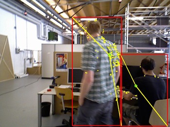
Boxes tracked by the box tracking method. The red boxes are the bounding boxes; the yellow dots are the seed points; the green dot is the mean point; and the yellow lines indicates the vectors used to obtain the two corners of a bounding box.

7. Results and Discussions
The experimental results and the discussions relative to them are presented in this section. Several open source SLAM libraries are used to compare with the proposed approach. In addition, the box tracking accuracy test results are also presented.
7.1 Experimental setup
The experiments were conducted using both publicly available and self-collected RGB-D datasets, wherein the TUM dataset [Reference Sturm, Engelhard, Endres, Burgard and Cremers2], which is publicly made available, is used since the ground truths are provided for comparison and evaluation. In addition, the dataset involves dynamic objects, making it an ideal dataset to test the proposed approach. Ample number of algorithms being proposed, which are discussed in section 2, employs TUM dataset as well. For self-collected dataset, ZED stereo camera is used. ZED stereo camera is incorporated with a software development kit (SDK) which allows RGB-D data recording. Both indoor and outdoor datasets were recorded hand-held, where all the recorded dataset involved dynamic semantics in the scene. The image resolution of TUM dataset is
 $640 \times 480$
, while the ZED recorder images bear
 $672 \times 376$
resolution. ZED sequences were recorded at 15 frames per second (FPS).
Box tracking accuracy test results for boxes being tracked using seed points.

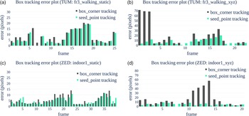
Error plots of tracking boxes using box-corner tracking method and box tracking using seed points for segments of four sequences (entitled in each plot). Here, the horizontal axis (labelled frame) is the number of frames in which the box is supposed to be tracked.

The experiments were performed using Intel i5–8250U CPU (1.6GHz) with 16GB memory. The dynamic objects in datasets are annotated to obtain a pre-trained model for the object detection module for detecting the semantics. For both training and detection, the TensorFlow object detection module [Reference Huang, Rathod, Sun, Zhu, Korattikara, Fathi, Fischer, Wojna, Song, Guadarrama and Murphy41] is employed. For tracking the features, KLT tracker is used. The masking parameters used in these experiments were kept constant. The masking image recalling factor
 $k$
is kept at 4 for all the experiments, hence reducing the resolution of the mask image by 4 times the original image.
7.2. Comparison specifications
The proposed approach is built on top of the RGB-D parallel tracking and mapping (RGBD-PTAM) implementation which is designed and developed based on S-PTAM [Reference Pire, Fischer, Civera, Cristóforis and Berlles9] algorithm. The comparison is performed using results obtained through ORB-SLAM2 [Reference Mur-Artal and Tardós8], RTAB-Map [Reference Labbé and Michaud42], RGBD-PTAM [Reference Pire, Fischer, Civera, Cristóforis and Berlles9] and the modified RGB-PTAM as the proposed approach. For TUM dataset, both static and dynamic scenes are utilized, whereas for self-collected dataset, indoor and outdoor data are collected to further test the mentioned approaches.
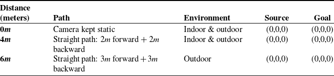
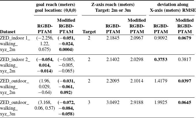
For self-collected dataset, no ground truth was collected, but a benchmark is set to compare the results wherein, a predefined path is defined. Table I shows the specifications of the benchmark set for the collected dataset. Both the path defined are straight paths, where the camera moves in a straight line for a specified distance from source at location, say
 $\left( {0,0,0} \right)$
in a 3D cartesian coordinate system and returns to
 $\left( {0,0,0} \right)$
. Therefore, it is expected for an algorithm to obtain a path that returns the camera’s location back to the source. In addition, since the camera moves back and forth in a straight line though hand-held, an algorithm is expected to produce a path close to straight line in a top-view (2D) mode. These two specifications – camera returning to source and camera following a straight 2D path – are used to compare the algorithms.
In addition, the box tracking module is tested using segments of both TUM and self-collected datasets, wherein the performance of box tracking is tested.
7.3. Evaluation of box tracking module
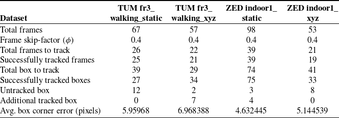
In this evaluation, dynamic objects in segments of both TUM and self-collected datasets are annotated to set a ground truth. In the experiments, the approach takes the RGB images along with annotated data as input. In the process, the annotations are randomly removed, simulating cases where the object detection module fails to detect a dynamic object. For any removed annotation or bounding box, it is expected for the box tracking method to track a box. Fig. 10 shows and illustration of the result obtained from tracking a box.
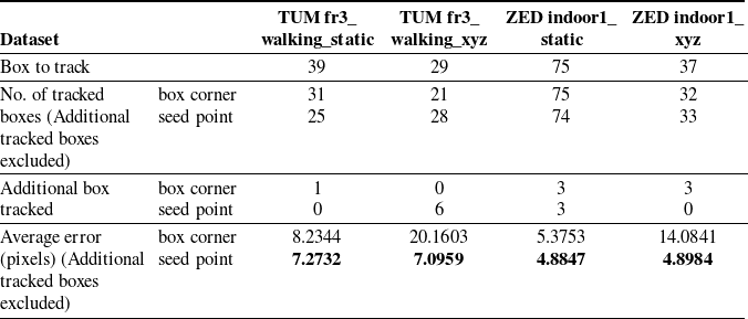
Comparison of tracking boxes using box-corner tracking method and box being tracked using seed points.

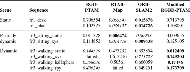
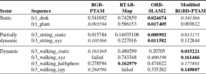
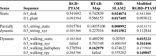
Comparison of root-mean-squared error (RMSE) of the absolute trajectory error (ATE) in meters for the trajectories obtained using RGBD-PTAM, RTAB-Map, ORB-SLAM2 and proposed approach (Modified RGBD-PTAM).

Comparison of translational relative pose errors (RPE) in meters obtained using RGBD-PTAM, RTAB-Map, ORB-SLAM2 and proposed approach (Modified RGBD-PTAM) over TUM RGB-D dataset sequences.

Comparison of rotational relative pose errors (RPE) in degrees obtained using RGBD-PTAM, RTAB-Map, ORB-SLAM2 and proposed approach (Modified RGBD-PTAM) over TUM RGB-D dataset sequences.

In this experiment, a frame skip-factor, say
 $\phi ,$
is used to define the percentage of frames in which the boxes are to be removed. In any given sequence, a random number of frame indices are selected based on
 $\phi $
where the bounding boxes are to be removed. The number of boxes being removed are recorded such that the number tracked boxes can be compared with it to obtain an accuracy scale. In addition, the distance between the corners of the ground truth boxes and tracked boxes are compared to evaluate the errors of the box being tracked. Table II shows the results obtained from segments of four sequences. It is observed that the method sometimes tracks additional boxes in cases where there are no expected boxes be tracked as per the ground truth data. The average box corner error (last row of Table II) is computed by first obtaining the difference between the ground truth and the tracked box, followed by computing average error as:
 \begin{equation}\varepsilon = \frac{1}{{4n}}\mathop \sum \limits_{i\;=\;1}^n \left( {{e_{x,min,i}} + {e_{y,min,i}} + {e_{x,max,i}} + {e_{y,max,i}}} \right)\end{equation}
where
 $n$
is the number of tracked boxes apart from the additional tracked boxes and the unit of
 $\varepsilon $
is in pixels. The term
 ${e_{x,min,i}}$
as computed as:
 \begin{equation}{e_{x,min,i}} = \left| {x_{min,i}^g - x_{min,i}^t} \right|\end{equation}
where
 $x_{min,i}^g$
and
 $x_{min,i}^t$
are the lower-limit or minimum
 $x$
component (along
 $x$
-axis) of the ground truth and the tracked box, respectively. The terms
 ${e_{y,min,i}}$
,
 ${e_{x,max,i}}$
and
 ${e_{y,max,i}}$
in Eq. (24) are computed in a similar manner.
The approach of tracking the boxes using seed points is further compared with the box tracked using the box corners. For tracking the corners, the two corners of a box, say
 ${\left( {{x_{min}},{y_{min}}} \right)_{{b_l}}}$
and
 ${\left( {{x_{max}},{y_{max}}} \right)_{{b_{l,}}}}$
are tracked and the obtained tracked points are compared with the ground truth box corners to obtain the error in pixels. In this test, at each random frame where the box is to be tracked, the sum of errors the two corners are considered. Fig. 11 shows the bar graph of the obtained error results for the same dataset segments used in Table II. Further results are presented in Table III. Here, the average errors are computed using the same approach as discussed for Table II. It is imperative to note that these results are obtained from randomly removing boxes from segments of the sequences, and it is observed that tracking boxes using seed points gave more consistent box tracking accuracies though the success rate of tracking box corners is also adequate.
7.4 Evaluation of the proposed approach and comparisons
The overall tests and experiments of the proposed approach are implemented using TUM RGB-D dataset and a set of self-collected dataset, which was collected using ZED stereo camera in both indoor and outdoor conditions. Tables IV, V and VI show the results and comparison of the proposed approach – which is built on top of RGBD-PTAM (hence named modified RGBD-PTAM in the tables) – against RGBD-PTAM, RTAB-Map and ORB-SLAM2 over a selected set of sequences from TUM dataset. This test is performed over static, partially dynamic and dynamic scenes using TUM benchmark. Table IV shows the root-mean-squared error (RMSE) of the absolute trajectory error (ATE) of the obtained trajectories in meters, while Tables V and VI show the translational relative pose error (RPE) in meters and rotational RPE in degrees, respectively. Here, as the proposed approach is built on top of RGBD-PTAM, the error value or rather, its accuracy depends on how well the base algorithm performs. While the modified RGBD-PTAM performs as the base algorithm in static and partially dynamic scenes, in dynamic scenes, the proposed approach mostly outperforms the other algorithms as they do not have modules that separately or particularly handles the dynamic objects. It is irrefutable from these results that filtering out the dynamic features can improve the overall SLAM performance. The trajectories obtained using the proposed approach over the dynamic scene sequences – used in Tables IV–VI – are shown in Fig. 12.
Plots comparing the trajectories obtained by the proposed approach (modified RGBD-PTAM) against the ground truth over the sequences (a) fr3_sitting_static, (b) fr3_sitting_xyz, (c) fr3_walking_static, (d) fr3_walking_xyz, (e) fr3_walking_halfsphere and (f) fr3_walking_rpy of TUM’s RGB-D sequences which involves partially dynamic and dynamic objects. The black line indicates ground truth the trajectory, the blue line is the estimated trajectory, and the red lines represent the difference between the ground truth and the estimated positions.

Due to the absence of ground truth for the dataset collected using ZED camera, the measures mentioned in section 7.2 are considered to test the accuracy of the proposed approach. The results are presented in Tables VII and VIII. The comparison of proposed approach against RGBD-PTAM – the base algorithm – for sequences where the camera is kept static is presented in Table VII. For static sequences, the RMSE of ATE is obtainable as it is expected for the algorithm to estimate the pose at the source, say
 $\left( {0,0,0} \right)$
throughout the sequence. For non-static sequences where the camera is in motion, a pre-defined path is followed wherein, all sequences follow a straight path as defined in Table I. The results obtained for the non-static camera sequences is presented in Table VIII.
Comparison of root-mean-squared error (RMSE) of the absolute trajectory error (ATE) in meters for the trajectories obtained using RGBD-PTAM and proposed approach (Modified RGBD-PTAM) for sequences collected using ZED stereo camera, where the camera was kept static. Comparison performed over both indoor and outdoor sequences.

Comparison of root-mean-squared error (RMSE) of the goal-reach, Z-reach and deviation along X-axis in meters obtained using RGBD-PTAM and proposed approach (Modified RGBD-PTAM) for sequences collected using ZED stereo camera, where the camera moved for specific distance. Comparison performed over both indoor and outdoor sequences. The Z-axis reach is defined based on how far the camera is intended to move in Z-axis, while X-axis deviation defines how far the camera deviates along the X-axis. The intended path follows straight path in the Z-axis.

In Table VIII, the
 $Z$
-axis reach defines how far the camera is expected to move based on the pre-defined path along the camera’s
 $Z$
-axis. For example, as per Table I, the two pre-defined
 $Z$
-axis targets are
 $2meters$
and
 $3meters$
and as the camera moves back and forth, the camera is expected to move back after reaching the
 $Z$
-axis target. The deviation along
 $X$
-axis defines how far the camera moves away from the camera’s
 $Z$
-axis at each timestamp. As the intended path is a straight line, the deviation in the
 $X$
-axis is expected to be minimal. In other words, the location of camera along
 $X$
-axis is expected to be constant, that is
 ${x_i} \approx 0$
throughout the sequence. The more deviation, the more erroneous the trajectory.
The 2D trajectory plots are presented in Fig. 13 over the non-static sequences. From these plots, it is observable that dynamic objects can cause drifts in the trajectory. It is also observed that the drift tends to occur in the direction of the moving objects. From these plots, it is observable that the proposed approach keeps the camera close to the intended path by negating the effects of dynamic objects by a considerable degree, unlike the trajectories obtained by RGBD-PTAM where there are significantly larger drifts.
2D plot of trajectories obtained by RGBD-PTAM (green) and proposed approach (orange) compared against the intended straight-line path over sequences collected using ZED stereo camera (ZED_indoor1_xyz_2m, ZED_indoor2_xyz_2m, ZED_outdoor_xyz_2m and ZED_outdoor_xyz_3m).

8. Conclusions
This paper presents modules that can be incorporated into a SLAM algorithm to improve its performance in a dynamic environment. The proposed approach detects semantics and classifies the semantics based on how likely they belong to a dynamic object class. A depth-first search (DFS)-based depth masking method is introduced which takes the depth image and the detected bounding boxes to generate a lower resolution binary mask image, which is then used to segment or separate features into three classes – valid features, seed points and invalid points. The valid features, which belong to static background are used for performing SLAM, and the invalid points are eliminated, while the seed points – point features which belongs to the mask – are tracked to assist in regenerating masks as well as track boxes to obtain consistent masking.
The proposed approach was built over a state-of-the-art SLAM algorithm RGBD-PTAM, and the experiments were implemented over the TUM RGB-D dataset and sequences collected using ZED stereo camera, where both indoor and outdoor data were collected. Other state-of-the-art SLAM algorithms, particularly RTAB-Map, ORB-SLAM including RGBD-PTAM, are compared against the proposed approach over the TUM RGB-D dataset and further evaluated over the ZED sequences. While TUM RGB-D sequences are recorded indoors, the self-collected dataset includes outdoor sequences as well. In order to test the versatility of the proposed algorithm. The results show that incorporating the proposed approach improves the overall output of the SLAM algorithm in dynamic environments, nullifying the effects of moving objects substantially.
Based on experiments conducted and also the results presented in Tables IV–VI, ORB-SLAM2 carries favourable accuracies. Incorporating the proposed approach into other adequately performing algorithms is a future perspective. The proposed approach is designed for RGB-D data and hence limited to RGB-D images. Integrating some of the concepts into SLAM algorithms which utilizes other type of input data is also a possible future work.
Acknowledgements
This work is supported by NavAjna Technologies Pvt. Ltd., Mercedes-Benz Research & Development India and Indian Institute of Information Technology, Allahabad.
Disclosure Statement
This manuscript is original, has not been published previously and not under consideration for publication elsewhere. Additionally, to the best of our knowledge, the named authors have no conflict of interest, financial or otherwise.
Author Contributions
The study is conceived designed by both the authors – L. Kenye and R. Kala. L. Kenye conducted the data gathering, development and experiments, while R. Kala involved in the evaluations. The article is written and arranged by both the authors.