INTRODUCTION
Mathematical functions have been used to describe growth of domestic ruminants for predictive purposes, and the information can be used at both scientific and farm levels. The parameters that constitute the non-linear mathematical functions are artefacts of the human mind, but they are useful representations of reality. Researchers ideally take random, unbiased samples for point and interval estimation of parametric values and make inferences to the population of interest. Therefore, parameters of traditional growth functions are empirical and can be aggregated, for instance, at the organism level; they have been used to summarize information about the growth profile into a few terms such as the specific growth rate, weights at birth and maturity and residual variance. Nonetheless, advances in computational statistics have been introduced into statistical software (Pinheiro & Bates Reference Pinheiro and Bates2000; Littell et al. Reference Littell, Milliken, Stroup, Wolfinger and Schabenberger2006; Vonesh Reference Vonesh2012) that allow a more general quantitative description of growth by generalizing not only the expected growth mean, but also the variance of growth trends, thus accommodating heteroscedasticity of the growing variable over time.
The growth of ruminants is centripetal, i.e., the head and foreparts achieve asymptotic growth prior to inner body counterparts (Lawrence & Fowler Reference Lawrence and Fowler2002). However, in goat wethers, as with other castrated farm ruminants, the long bones probably reach a greater length compared with intact animals, but hormones other than oestrogen and testosterone (e.g., thyroid hormones and growth factors) may act as determinants of complete ossification of epiphyseal plates after puberty (Doumit & Merkel Reference Doumit, Merkel, Pond and Bell2005; Hossner Reference Hossner2005). In general, weight records of ruminants resemble a sigmoid-shaped pattern, and body parts such as bones, muscles and fat exhibit remarkable differences in their growth profiles. Whenever detected in the growth profile, the inflection point is usually attributable to puberty, the point at which sexual maturity begins and the growth rate starts to reduce asymptotically to zero. The maturity of these major body constituents occurs earlier for bones, intermediate for muscles and later for fat with reference to the timing of body maturity (Doumit & Merkel Reference Doumit, Merkel, Pond and Bell2005). Nevertheless, how body parts and body composition change from birth to maturity in goats remains unknown. The distribution of fat in the bodies of goats differs from that of other ruminant species, and visceral fat accretion is a striking characteristic that may help goats to survive and even reproduce in the face of seasonal food shortages (Carmichael et al. Reference Carmichael, Kouakou, Gelaye, Kannan, Lee and Terrill2012). Despite the fact that castrated animals usually have intermediary growth profiles when compared with intact males and females (Mahgoub et al. Reference Mahgoub, Kadim, Al-Saqry and Al-Busaidi2004), the information gathered from wethers may be of use for predictive purposes and understanding long-term variation. Therefore, based on a multi-model selection process, the goal of the present study was to characterize the growth of body parts and composition of the growing empty body to infer how these aspects relate to the long-term growth of goat wethers from specialized dairy breeds.
MATERIALS AND METHODS
Swiss Alpine (Chamoisée) and Saanen kids used in the present study were sampled from the annual offspring of a large dairy herd raised in the county of Viçosa (20°46′22″ S, 42°51′12″ W, elevation 706 m a.s.l.), State of Minas Gerais (Brazil), where according to the Köppen–Geiger classification (Kottek et al. Reference Kottek, Grieser, Beck, Rudolf and Rubel2006), a Cwa climate predominates (i.e. the main climate is warm temperate, with dry winters and hot summers). Two Saanen and two Alpine kids were sampled randomly and slaughtered at birth, and one Saanen and three Alpine kids were sampled at random and slaughtered at 15 days old. Afterwards, 50 kids (37 Alpine and 13 Saanen) were moved for rearing in the county of Campos dos Goytacazes (21°42′36″ S, 41°20′22″ W, elevation 15 m a.s.l.), Northern Rio de Janeiro State, where the predominant climate according to Köppen–Geiger classification (Kottek et al. Reference Kottek, Grieser, Beck, Rudolf and Rubel2006) is Aw (equatorial savannah with dry winters). The kids were castrated immediately after their arrival.
The kids were reared in a floor-bed-type barn until weaning at 90 days old. A milk replacer was fed, and a soybean meal and ground maize mixture was offered to the animals on a daily basis. Cunhã (Clitoria ternatea, L.), Elephant-grass (Pennisetum purpureum, Schum.) and occasionally Sabiá (Mimosa caesalpiniifolia, Bentham) were the roughages available and offered ad libitum to the kids until weaning. After 90 days, four kids were chosen randomly and slaughtered; the remaining 46 kids were transferred to a stilted-type barn with a slatted floor and the animals received a ration based on soybean meal, ground maize, minerals and maize silage (Zea mays, L.). These 46 animals were divided into seven groups and each group was allotted to a pen (from five to seven animals per pen). However, it is important to emphasize that animals were group-fed the same experimental diet. Additional roughage (Cunhã, Elephant-grass and occasionally Sabiá) was offered ad libitum according to the availability of the forage type. The diet was formulated for a target average daily weight gain of 0·150 kg/day, based on tabular energy and chemical composition of feeds (AFRC 1997; NRC 2007) programmed in a non-linear optimization algorithm used to minimize the cost of the diet (Jardim et al. Reference Jardim, Vieira, Fernandes, Araujo, Glória, Rohem Júnior, Rocha and Abreu2013, Reference Jardim, Vieira, Fernandes, Araujo, Glória, Rohem Júnior, Rocha and Abreu2015). The amount of concentrate offered was adjusted monthly after weaning as the animals grew and according to the forage type available. The dry matter (DM) intake of concentrate scaled to the metabolic body weight (BW0·75) at weaning averaged (mean ± s.d.) 34 ± 0·2 g/(day × kg0·75). The concentrate used (crude protein (CP) = 191 g/kg; metabolizable energy = 11·3 MJ/kg) contained 283·5 g of soybean meal, 575·3 g of ground maize and 29·7 g of mineral pre-mix per kg dry matter. The BW0·75 scaled intake rate of DM averaged (mean ± s.d.) 62 ± 3·6 g/(day × kg0·75) from 135 to 365 days, dropped to 42 ± 6·4 at 485 days and 37 ± 5·9 at 545 days, and stabilized at 36 ± 3·6 g/(day × kg0·75) from 610 to 890 days of the experimental period.
In addition to birth (day zero) and to 15 days of age, the animals were slaughtered at approximate ages of 90 (weaning), 135, 210, 270, 365, 485, 610, 735, 790, 840, 890 and 920 days. Nonetheless, the growth profiles were obtained with the actual age at slaughter for each animal to avoid bias in the resulting growth profiles. The oldest ages (790–920 days old) at slaughter were chosen at the time of replacement of the last deciduous incisive teeth. Four animals were slaughtered at each age, except at later ages when the remaining animals were slaughtered. Half of the animals were slaughtered 2 h after the morning meal and the other half 2 h after the afternoon meal to measure the contents of the full gastrointestinal tract. At slaughter, the animals were rendered insensible, bled, flayed and eviscerated. Individual parts, i.e. the head, members, half carcasses, blood, skin, organs (including the remaining reproductive tract and bladder), the segments of the gastrointestinal tract and their contents, total abdominal fat (omental, pelvic and renal), and trimmed cuts (diaphragm, non-carcass muscle pieces and thymus) were weighed to the nearest 0·005 kg. All body parts, including carcass, head and members, were ground in a cutter mill.
Chemical analyses
Samples of the body parts were dried at 55 °C, and except for blood and skin samples, the excess fat from the dried samples was removed by petroleum ether extraction in a large volume (500 ml) Soxhlet apparatus before further analysis. The skin and de-fatted samples were ball-milled and their DM (method 967·03; AOAC 1998), CP (method 2001·11; Thiex et al. Reference Thiex, Manson, Andersson and Persson2002), crude fat (CF, method 2003·06; Thiex et al. Reference Thiex, Anderson and Gildemeister2003) and ash (Ash; method 942·05; AOAC 1998) contents were determined. The energy content of the body was computed from the caloric equivalents of protein and fat, i.e., 23·4 and 39·3 MJ/kg, respectively (Maynard et al. Reference Maynard, Loosli, Hintz and Warner1979). The DM, CP, CF, Ash and energy contents were computed as empty body weight (EBW), namely EBDM, EBCP, EBCF, EBAsh and EBE. The water content of the EBW was computed as EBH2O = EBW – EBDM.
Growth and covariance models
The general structure attributed to the growth models was
 $Y_t = \mu _{Y_t} + e_t $
, for
 $Y_t \sim Normal(\mu _{Y_t}, \sigma _{Y_t} ^2 )$
, i.e., the variable Y
t
is assumed to follow a normal distribution with mean and variance functions
 $\mu _{Y_t} $
and
 $\sigma _{Y_t} ^2 $
, respectively, as follows:
 $$\mu _{Y_t} \, = \,Y_f - b\exp (\! - kt)$$
 $$\mu _{Y_t} \, = \,Y_0 \exp (k(1 - \exp ( - Dt))/D)$$
 $$\mu _{Y_t} \, = \,Y_0 \times Y_f /(Y_0^n + (Y_f^n - Y_0^n )\exp ( - kt))^{1/n}$$
and
 $$\mu _{Y_t} = Y_{\,f1} - b\exp ( - k_1 t) + Y_{20} \exp (k_2 (1 - \exp ( - Dt))/D)$$
No random factors were introduced in the models excepting the assumed independently distributed error term, i.e.,
 $e_t \sim {\rm Normal}\,(0,\sigma _t^2 )$
. Equation (1) represents monomolecular growth (Brody Reference Brody1945; France et al.
Reference France, Dijkstra and Dhanoa1996), in which Y
f
is the asymptotic weight at maturity (mass units), k is the first-order specific growth rate (1/day) and b is a scale parameter. Equation (2) is the well-known Gompertz model and its parameters Y
0, k and D are the intercept (mass units), specific growth rate (1/day) and fractional reduction rate of the specific growth rate (1/day), respectively (France et al.
Reference France, Dijkstra and Dhanoa1996). The model proposed by Richards (Reference Richards1959), or Eqn (3), is the general model used as a reference for describing growth. In Eqn (3), Y
0 is the intercept, Y
f
is the asymptotic growth parameter, k is the specific growth rate and n is a size-scaling-related parameter that could be constrained, for instance, by the metabolic body size. The monomolecular or Brody growth model is combined with the Gompertz model to form the biphasic function shown by Eqn (4), in which Y
f1 is a scale parameter (mass units) representing the asymptotic phase of the monomolecular growth phase, b is a scale parameter (mass units) and k
1 (1/day) is the specific growth rate of the first-order initial growth. The parameter Y
20 (mass units) is a scale parameter representing the intercept of the sigmoid phase of growth, and k
2 and D, both expressed as 1/day, are the specific growth rate and its fractional rate of reduction during the sigmoid growth phase, respectively (Rocha et al.
Reference Rocha, Vieira, Abreu, Araujo, Glória, Tamy, Camisa Nova and Fernandes2015).
The conventional assumption of homoscedasticity was challenged using the computational powers of the NLMIXED procedure of SAS (v.9, SAS Systems, Inc., Cary, NC, USA). Attempts were made to correct for heterogeneity of variances over time in non-linear parameter estimation, such as weighted least squares (Matis & Hartley Reference Matis and Hartley1971; Bard Reference Bard1974). Only recently, however, has the computational analysis been improved by the powers of hardware and software to allow a widespread use of maximum-likelihood estimation of non-linear models and covariance structures that accommodate heteroscedasticity (Pinheiro & Bates Reference Pinheiro and Bates2000; Littell et al. Reference Littell, Milliken, Stroup, Wolfinger and Schabenberger2006; Vonesh Reference Vonesh2012). Hence, the variance was modelled as follows:
 $$\sigma _{Y_t} ^2 = \sigma ^2 $$
 $$\sigma _{Y_t} ^2 = \sigma _0^2 \exp \,(ct)$$
 $$\sigma _{Y_t} ^2 = \sigma _0^2 + \sigma _b^2 (1 - \exp \,( - st))$$
and
 $$\sigma _{Y_t} ^2 = \sigma ^2 (\mu _{Y_t} )^{2\psi} $$
where σ
2 is the homogeneous residual variance (
 $\sigma _t^2 = \sigma ^2 $
) as shown by Eqn (5). Exponential variance or Eqn (6) contains the starting residual variance (
 $\sigma _t^2 = \sigma _0^2 $
) associated with the weight at birth (t = 0), which increases exponentially during growth at a fractional rate c (1/day). Equation (7) describes an asymptotically growing variance, in which
 $\sigma _t^2 = \sigma _0^2 $
as the variance related to weights at birth,
 $\sigma _b^2 $
is the asymptotic increase in variance over time, and s (1/day) is the fractional rate or first-order rate of increase in
 $\sigma _{Y_t} ^2 $
. Equation (8) represent the residual variance (
 $\sigma _t^2 = \sigma ^2 $
) scaled by a power (ψ) function the expected mean,
 $\mu _{Y_t} $
.
The profiles exhibited by some variables measured in the present study resembled a straight line. In this regard, a simple linear model was introduced as Eqn (9) in order to check whether a linear model was as likely to describe the growth patterns as Eqns (1)–(4):
 $$\mu _{Y_t} \, = \,\beta _0 + \beta _1 t$$
The parameters β
0 and β
1 are the intercept and the slope of the growth profile, respectively. This model was also fitted in combination with Eqns (5)–(8). In addition, the effect of genotype was accounted for by introducing the fixed effect of breed (Alpine and Saanen) to evaluate the influence of breed over parameters according to the recommendations specified by Littell et al. (Reference Littell, Milliken, Stroup, Wolfinger and Schabenberger2006) and Vonesh (Reference Vonesh2012). Therefore, 40 models were tested: 20 models were produced by evaluating five models to interpret the expected growth (
 $\mu _{Y_t} $
) multiplied by four types of variance functions (
 $\sigma _{Y_t} ^2 $
), without the breed effect; and 20 model combinations
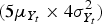 $(5\mu _{Y_t} \times 4\sigma _{Y_t} ^2 )$
were evaluated by introducing the fixed effect of breed.
Statistical procedures
The 40 models were fitted to the growth profiles by using the NLMIXED procedure of SAS (v.9, SAS Systems, Inc., Cary, NC, USA). The chosen Newton–Raphson algorithm (tech = NEWRAP) solved the maximum-likelihood estimation method by combining line search with ridging. The Akaike information criterion (Akaike Reference Akaike1974), corrected for small samples (Sugiura Reference Sugiura1978), is an output of the NLMIXED procedure. Therefore, the derived likelihood criteria were computed to establish a framework of multi-model selection (Burnham & Anderson Reference Burnham and Anderson2004). The corrected Akaike criterion, namely AICc r , computed for the rth model in the set of 40 models was used to calculate the differences (Δ r ) between the rth model and the minimum AICc r computed in the set of 40 models fitted. A likelihood probability w r (or Akaike weight) was computed for each one of the 40 models fitted. The evidence ratio ER r was computed from the maximum w r in the set of models fitted and the respective w r value of rth fitted model under evaluation. Models that presented 0 ⩽ Δ r ⩽ 2 also presented higher w r and lower ER r values and were therefore considered the best choice, given the data. Models with 2 < Δ r ⩽ 8 were considered to have less support, and models with Δ r > 8 were considered the worst choices among the evaluated models. The number of parameters (Θ) was considered as an additional parsimony criterion whenever the models were equally likely (i.e., for w r computed in the range 0 ⩽ Δ r ⩽ 2), and the model with a smaller number of parameters was preferably chosen (Burnham & Anderson Reference Burnham and Anderson2004). A full rank covariance matrix for parameters is indicative of a well-conditioned model, produces reliable covariance parameter estimates at convergence and is obtained in the fitting process whenever a positive definite Hessian is achieved (Pinheiro & Bates Reference Pinheiro and Bates2000). Therefore, the output of a full rank covariance matrix was considered a distinguishing criterion prevailing over the other criteria. This means that the model chosen in the set of possible models was the one which presented a full rank covariance matrix, equally likely information criteria and the lowest Θ.
One of the advantages of the NLMIXED procedure is the capability of predicting any function of the model parameters and performing tests on the general non-linear hypothesis, i.e., that any function
 $\hat g(\hat \theta, \; t)$
of the parameters can be predicted (Littell et al.
Reference Littell, Milliken, Stroup, Wolfinger and Schabenberger2006; Vonesh Reference Vonesh2012). The average daily rate of mass accretion (ΔY
t
/Δt) can be listed as an example. Therefore, based on the estimated covariance matrix of Y
t
and parameter estimates given the data, reliable confidence intervals (99%CI) were estimated for
 $\hat g(\hat \theta, \; t)$
and figure in the output of NLMIXED as
 $$99\% {\rm CI}:\hat g(\hat \theta, \; t) \pm t_{\left( {1 - \alpha, \; \; df} \right)} SE_{\hat g(\hat \theta, \; t)} $$
The estimate
 $SE_{\hat g(\hat \theta, \; t)} $
is the standard error of the estimate
 $\hat g(\hat \theta, \; t)$
; t
(1−α, df) is the two-tailed critical value of the Student's-t distribution based on the adopted significance level P < 0·01 and the degrees of freedom used to compute the estimate, df = n − Θ for n representing the number of observations and Θ corresponding to the number of parameters of
 $\hat g(\hat \theta, \; t)$
, including the variance parameters of Eqns (5)–(8). Therefore,
 $SE_{\hat g\left( {\hat \theta, \; t} \right)} $
can be obtained easily by dividing the reported quantity
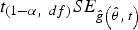 $t_{\left( {1 - \alpha, \; \; df} \right)} SE_{\hat g\left( {\hat \theta, \; t} \right)} $
by t
(1−α, df). The inflection points of Eqns (2) and (3) can be calculated by equating to zero the respective second derivatives and solving for t algebraically (France et al.
Reference France, Dijkstra and Dhanoa1996), or in the case of Eqn (4), numerically (Rocha et al.
Reference Rocha, Vieira, Abreu, Araujo, Glória, Tamy, Camisa Nova and Fernandes2015).
Reference inflection point
Inflection points were not detected in the growth profiles of BW and EBW. Therefore, the proportion of weight at maturity at the inflection point reported by Regadas Filho et al. (Reference Regadas Filho, Tedeschi, Rodrigues, Brito and Oliveira2014) was used, because those authors fitted the Richards model to the growth of females from birth to maturity, and those females were a representative part of the herd that gave birth to the kids used in the present study. Therefore, based on Regadas Filho et al. (Reference Regadas Filho, Tedeschi, Rodrigues, Brito and Oliveira2014) estimates, both Swiss Alpine (Chamoisée) and Saanen doelings reach 40% of the asymptotic weight at the inflection point, i.e., approx. 20 kg. The 99%CI for the age (
 $t_i^{\prime} $
) at this mass was computed from the following
 $\hat g(\hat \theta, \; t)$
of the growth profile of BW in the present study:
 $$99\% {\rm CI}\,[t_i^{\prime} ]: - \ln ((Y_f - 20)/b)/k \pm t_{\left( {1 - \alpha, \; \; df} \right)} SE_{t_i^{\prime}} $$
Body composition
As will be seen in the Results section, the model that best represented both BW and EBW mass accumulations was Eqn (1) combined with Eqn (6). Therefore, to represent body composition as a proportion of body parts and chemical composition of BW and EBW, the following ratio was estimated:
 $$y^{\prime} = Y_t /X_t $$
for Y t representing mass of some body part or chemical constituent. The expected y′ was multiplied by 1000 to express results as g/kg of X t = BW or X t = EBW; for Y t representing empty body energy, y′ was expressed as MJ/kg of BW or EBW. Nonetheless, the ratio between two normally distributed variables has a Cauchy distribution, which has no mean and neither the higher moments (Mood et al. Reference Mood, Graybill and Boes1974). Because the Box–Cox transformation (Box & Cox Reference Box and Cox1964) is useful to correct for lack of normality (Peltier et al. Reference Peltier, Wilcox and Sharp1998), the TRANSREG procedure of SAS was used to obtain a suitable transformation for Eqn (12). As a result, the value of the parameter λ of the Box–Cox transformation that maximized the logarithm of the likelihood function for every single ratio based on Eqn (12) of the present study was zero. Therefore, y′ was transformed as
 $$y^T = \ln y^{\prime} = \ln (Y_t /X_t )\sim{\rm Normal}(\mu, \sigma ^2 )$$
Which means that the natural logarithm (ln) of y′, namely yT
, was assumed to follow a normal distribution with mean μ and variance σ
2. Because
 $\hat \mu _{Y_t} $
,
 $\hat \sigma _{Y_t} ^2 $
,
 $\hat \mu _{X_t} $
and
 $\hat \sigma _{X_t} ^2 $
are already known from the models that presented Δ
r
= 0·0, and represent expected mean and variance of Y
t
(all variables except BW and EBW) and X
t
(BW and EBW), a direct estimation based on a function of
 $\hat \mu _{Y_t} $
,
 $\hat \sigma _{Y_t} ^2 $
,
 $\hat \mu _{X_t} $
and
 $\hat \sigma _{X_t} ^2 $
was computed as a 99%CI for Eqn (12). Because the variables Y
t
and X
t
are dependent on each other, the expected mean (E[Y
t
/X
t
]) and variance (V[Y
t
/X
t
]) of this ratio are given by the following approximations (Mood et al.
Reference Mood, Graybill and Boes1974):
 $$E[Y_t /X_t ] \approx \hat \mu _{Y_t} /\hat \mu _{X_t} - {\rm cov}\,[Y_t, X_t ]/\hat \mu _{X_t} ^2 + \hat \sigma _{X_t} ^2 \hat \mu _{Y_t} /\hat \mu _{X_t} ^3 $$
and
 $$\eqalign{V[Y_t /X_t ] & \approx (\hat \mu _{Y_t} /\hat \mu _{X_t} )^2 (\hat \sigma _{Y_t} ^2 /\hat \mu _{Y_t} ^2 + \hat \sigma _{X_t} ^2 /\hat \mu _{X_t} ^2 \cr & \quad- 2{\rm cov}\,[Y_t, X_t ]/(\hat \mu _{Y_t} \hat \mu _{X_t} ))}$$
in which
 ${\rm cov}\,[Y_t, X_t ] = \rho _{Y_t, X_t} \hat \sigma _{Y_t} \hat \sigma _{X_t} $
. Note that the correlation between Y
t
and X
t
 $(\rho _{Y_t, X_t} )$
is the only parameter that remains unknown. If yT
is normally distributed as stated in Eqn (13), then it was implicitly assumed that the ratio Y
t
/X
t
follows a lognormal distribution with mean and variance given by Eqns (16) and (17).
 $$E[Y_t /X_t ] = \exp \,(\mu + \sigma ^2 /2)$$
 $$V[Y_t /X_t ] = \exp \,(2\mu + 2\sigma ^2 ) - \exp \,(2\mu + \sigma ^2 )$$
The solutions for μ and σ 2 were obtained algebraically by equating Eqns (14)–(16), and Eqns (15)–(17), and solving for μ and σ 2:
 $$\mu \approx \ln \,(\hat \mu _{Y_t} /\hat \mu _{X_t} - \rho _{Y_t, X_t} \hat \sigma _{Y_t} \hat \sigma _{X_t} /\hat \mu _{X_t} ^2 + \hat \sigma _{X_t} ^2 \hat \mu _{Y_t} /\hat \mu _{X_t} ^3 ) - {\sigma ^2}/2$$
and
 $$\eqalign{\sigma ^2 \, \approx \, & \ln \,(1 + (\hat \mu _{Y_t} /\hat \mu _{X_t} )^2 (\hat \sigma _{Y_t} ^2 /\hat \mu _{Y_t} ^2 + \hat \sigma _{X_t} ^2 /\hat \mu _{X_t} ^2 \cr &\quad- 2\rho _{Y_t, X_t} \hat \sigma _{Y_t} \hat \sigma _{X_t} /(\hat \mu _{Y_t} \hat \mu _{X_t} )) \cr & \times \exp \,( - 2\ln \,(\hat \mu _{Y_t} /\hat \mu _{X_t} - \cr &\qquad\rho _{Y_t, X_t} \hat \sigma _{Y_t} \hat \sigma _{X_t} /\hat \mu _{X_t} ^2 + \hat \sigma _{X_t} ^2 \hat \mu _{Y_t} /\hat \mu _{X_t} ^3 )))} $$
Therefore, the NLMIXED procedure was used to predict E[Y
t
/X
t
] by ascribing yT
~Normal (μ, σ
2) to the model sentence (MODEL) of the procedure. The estimated parameters of
 $\hat \mu _{Y_t} $
,
 $\hat \sigma _{Y_t} ^2 $
,
 $\hat \mu _{X_t} $
and
 $\hat \sigma _{X_t} ^2 $
were used as constants in the programming sentences of the NLMIXED procedure and the NEWRAP algorithm was allowed to run in order to estimate the parameter
 $\rho _{Y_t, X_t} $
. Once estimated, the correlation
 $\hat \rho _{Y_t, X_t} $
was added to the set of parameters (PARMS) involved in the estimation process, i.e., the parameter estimates of
 $\hat \mu _{Y_t} $
,
 $\hat \sigma _{Y_t} ^2 $
,
 $\hat \mu _{X_t} $
and
 $\hat \sigma _{X_t} ^2 $
, and the NLMIXED procedure was allowed to run without the optimization technique (TECH = NONE) with the augmented set of parameters (PARMS) due to the addition of
 $\hat \rho _{Y_t, X_t} $
. The degrees of freedom were computed accordingly.
Direct scaling of chemical components
The growth profiles of some chemical constituents were also represented graphically by simply plotting observed values and the respective estimated 99%CI of some variables against the expected EBW and EBCP, as follows:
 $$\hat \mu _{Y_t} \pm t_{\left( {1 - \alpha, \; \; df} \right)} SE_{\hat \mu _{Y_t}} = \hat \mu _{X_t} $$
and
 $$Y_t = \hat \mu _{X_t} $$
in which Y
t
= EBCP, EBCF, EBAsh or EBE for X
t
= EBW, and Y
t
= EBCF, EBAsh, EBE or EBH2O for X
t
= EBCP.
 $\hat \mu _{Y_t} $
and
 $\hat \mu _{X_t} $
were the fitted models chosen among Eqns (1)–(9) according to the quality-of-fit criteria previously described. The parabola or Eqn (22) has been successfully applied to scale Y
t
to X
t
(Brody Reference Brody1945), and has been used for predicting body composition and composition of gain (NRC 1996). By assuming that
 $Y_t \sim{\rm Normal}\,(\mu _{Y_t}, \sigma _{Y_t} ^2 )$
,
 $$\mu _{Y_t} = \gamma X_t^\delta $$
and
 $\sigma _{Y_t} ^2 $
follows Eqns (5), (6) or (8) after replacing t by X
t
(BW or EBW, kg). The breed effect was not accounted for in the scaling relationships. The best combination of Eqn (22) with the variance equation counterpart was chosen based on the same AICc
r
and derived likelihood-information measures as previously described. The average rates of mass or energy accretions (ΔY
t
/ΔX
t
) at specific mass intervals were computed as an additional
 $\hat g(\hat \theta, \; X_t )$
to be estimated as a 99%CI:
 $$\eqalign{99\% {\rm CI}\,[{\rm \Delta} Y_t /{\rm \Delta} X_t ] : & \gamma (\hat \mu _{X_{t^{\prime}}} ^\delta - \hat \mu _{X_t} ^\delta )/(\hat \mu _{X_{t^{\prime}}} - \hat \mu _{X_t} ) \cr & \quad \quad \pm t_{\left( {1 - \alpha, \; \; df} \right)} SE_{{\rm \Delta} Y_t /{\rm \Delta} X_t}}$$
for t′ > t.
 $\hat \mu _{X_{t^{\prime}}} $
and
 $\hat \mu _{X_t} $
are the expected X
t
masses at t′ and t, respectively. Parameter estimates were not shown because the purpose here was inferences on ΔY
t
/ΔX
t
. The age intervals chosen represent the early suckling phase (0–15 days), the adaptation period to a solid diet until weaning (15–90 days), and the post-weaning period until 7 months, which is the age at which replacement doelings of dairy breeds are mated to give birth at 1-year-old (Morand-Fehr & Sauvant Reference Morand-fehr, Sauvant and Jarrige1988). The rates were additionally estimated from one to two (365–730 days) and from two to almost two and half years old (730–913 days). The same age intervals were also used to estimate ΔY
t
/ΔX
t
as Eqn (10).
RESULTS
Selection of the best model
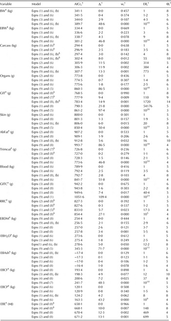
Because of the lack of information between 15 and 90 days, the estimation of the standard error of the parameter k 1 of Eqn (4) presented numerical problems and did not converge into a limit, i.e., tended to infinity. All the remaining parameters of this equation presented point and interval estimates. Therefore, to fit this equation more accurately, the starting value for k 1 was set equal to one because of the assumption that the monomolecular growth phase might have occurred during the initial stages of growth soon after birth. Nevertheless, this model did not present favourable likelihood criteria, did not present a full rank covariance matrix at convergence and was a worse choice for all cases (Table 1).
Some goodness-of-fit measures for models fitted* to the growing body, body parts and chemical constitution of the body of castrated male goats

† AICc r , corrected Akaike information criterion of the rth model; Δ r , difference between the AICc r values; w r , likelihood probability of the rth model; ER r , evidence ratio against the rth model; Θ r , number of parameters of the rth model.
‡ BW, body weight; EBW, empty body weight; GIT, gastrointestinal tract weight; AbFat, weight of the abdominal fat; Trimcut, weight of the trimmed cuts; GITC, weight of the fresh gastrointestinal contents; RRC, weight of the fresh ruminoreticular contents; and EBDM, EBH2O, EBAsh, EBCF, EBCP and EBE are the amounts of dry matter, water, ash, crude fat, crude protein and energy in the empty body, respectively.
§ The Hessian was not positive definite and the covariance matrix was not of full rank.
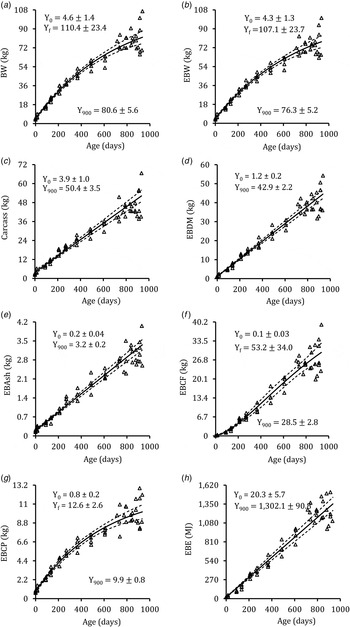
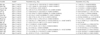
Some variables were fitted in grams (g) and other variables were fitted in kg because scale interfered in convergence during the optimization process. The models in which the breed effect was accounted for did not present favourable values for information-likelihood criteria. The exception was the best model for BW, i.e., Eqn (1) combined with Eqn (6), which also presented a full rank covariance matrix at convergence (Table 1). Nevertheless, despite the lowest Δ r and highest w r , there was no relevant numerical difference between the ERr values for Eqn (1) and (6) with and without the breed effect. Therefore, based on the additional parsimony criterion regarding the number of parameters, the best representation of BW was Eqn (1) combined with Eqn (6) without the breed effect (Table 2 and Fig. 1).
Observed (△), expected (solid lines) and 99% confidence intervals (99%CI, dashed lines) of the growth profiles, and 99%CI as Eqn (10) for the intercept (Y 0), asymptotic (Y f ) and 900-days (Y 900) masses. Dependent variables and the respective fitted models are: (a) body weight (BW, kg), Eqn (1) combined with Eqn (6); (b) empty body weight (EBW, kg), Eqn (1) with Eqn (6); (c) carcass weight (Carcass, kg), Eqn (9) with Eqn (6); and retained amounts in the empty body of (d) dry matter (EBDM, kg), Eqn (9) with Eqn (8); (e) ash (EBAsh, kg), Eqn (9) with Eqn (8); (f) crude fat (EBCF, kg), Eqn (3) with Eqn (8); (g) crude protein (EBCP, kg), Eqn (1) with Eqn (6); and (h) energy (EBE, kg), Eqn (9) with Eqn (8). Details of Eqns (1)–(9) are given in the text.

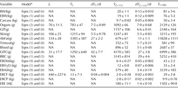
Estimates of parameters and its respective standard errors (SEθ) of the most likely model for each measured variable. The introduction of the breed effect did not improve the quality of fit and the models listed do not contain the breed effect

BW, body weight; EBW, empty body weight; GIT, gastrointestinal tract weight; AbFat, weight of the abdominal fat; Trimcut, weight of the trimmed cuts; GITC, fresh weight of the gastrointestinal contents; RRC, fresh weight of the ruminoreticular contents; empty body amounts of dry matter (EBDM), water (EBH2O), ash (EBAsh), crude fat (EBCF), crude protein (EBCP) and energy (EBE).


Equation (1) without the breed effect was the best choice for another seven variables of the 17 variables studied, and all parameter estimates of the chosen models presented reliable standard errors, with exception of RRC (Table 2). Equation (2) without the breed effect was unequivocally the best choice for three variables; Eqn (3) without the breed effect best mimicked the profiles of another two variables, and the linear model or Eqn (9) without the breed effect best fitted the growth profiles of four variables (Tables 1 and 2).
The traditional assumption of homoscedastic variance or Eqn (5) was not suited for representing the variability observed in the growth profiles of the majority of the variables studied. The exception was RRC, but none of the models fitted to RRC yielded full rank covariance matrices after convergence (Table 1) and the reported SE θ = b was not reliable (Table 2). Equation (6) modelled the variance of eight variables most closely, and Eqn (8) better represented the variance of the remaining eight variables. The asymptotic variance or Eqn (7) was not likely to represent the variability of any variable in the set (Table 2).
Long-term growth
Graphs were built to illustrate point and interval estimates for
 $\mu _{Y_t} $
of some variables in the continuum of the time-axis (Fig. 1). It should be noted that visually well-defined asymptotes were not reached for the selected variables. Figure 1 also contains the 99%CI of the intercept and asymptote of the estimated functions, thus indicating masses at birth and close to maturity. Some limits of the growth functions yielded estimates at maturity that are likely to occur; nonetheless, as mentioned before, some asymptotic values were overestimated or did not present asymptotic masses at all, as indicated by the linear profiles (Table 2). Thus, for some variables, asymptotic masses as estimates of the weights at maturity were less likely and a well-defined asymptote had not been reached. On the contrary, if
 $0.95\hat Y_f $
or
 $0.95\hat Y_0 \exp \,(\hat k/\hat D)$
at 913 days old were reached then it was possible to assume that asymptotic growth had been achieved. Based on Tables 2 and 3, variables that satisfied this simple condition were Organs, GIT, Skin, AbFat, Trimcut, GITC and RRC.
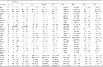
Estimated 99% confidence intervals (99%CI) presented as
 $\hat g(\hat \theta, \; t) \pm t_{\left( {1 - \alpha, \; \; df} \right)} SE_{\hat g(\hat \theta, \; t)} $
for proportions of body parts and chemical constituents* of the body weight (BW, kg) and empty body weight (EBW, kg) based on fitted equations at specific ages

Carcass; organs; GIT, gastrointestinal tract weight; Skin; AbFat, weight of the abdominal fat; Trimcut, weight of the trimmed cuts; GITC, fresh weight of the gastrointestinal contents; and RRC, fresh weight of the ruminoreticular contents. These variables are expressed in g/kg of the respective heading variable: BW or EBW.
* Empty body concentrations of dry matter (EBDM), water (EBH2O), ash (EBAsh), crude fat (EBCF) and crude protein (EBCP) are expressed in g/kg, and energy (EBE) expressed in MJ/kg of the respective heading variable: BW or EBW.
† 99%CI for the age at the inflection point for dairy does based on parameter estimates reported by Regadas Filho et al. (Reference Regadas Filho, Tedeschi, Rodrigues, Brito and Oliveira2014).
‡ Degrees of freedom used to build the 99% CI.
The use of Eqns (14)–(19) allowed the estimation of proportions of body parts and chemical composition of BW and EBW at specific ages (Table 3). The proportions of RRC at t = 0 and 15 days old were small and thus excluded before fitting the models, which explains why the proportions at these ages were reported as negligible. Because EBCF growth was sigmoid and EBCP growth was monomolecular, fat deposition occurred later than protein deposition. At
 $\hat t_i^{\prime} $
, only 20·0/83·5 = 0·240 of BW at 913 days was achieved, and 210-day-old animals reached 31·6/83·5 = 0·379 of the 913-day-old BW. The inflection points detected for AbFat and EBCF (Table 4) are indications that fat was also deposited later than EBDM, EBAsh and EBH2O.
Estimates of the 99% confidence intervals presented as
 $\hat g(\hat \theta, \; t) \pm t_{\left( {1 - \alpha, \; \; df} \right)} SE_{\hat g(\hat \theta, \; t)} $
for ages at the inflection points
 $(\hat t_i {\rm, \; days})$
, variables at
 $\hat t_i $
(
 $\hat Y_{t_i} $
; g, kg or MJ), growth rates at
 $\hat t_i $
(
 $d\hat Y_{t_i} /dt$
; g, kg or MJ/day),
 $\hat Y_{\hat t_i^{\prime}} $
and
 $d\hat Y_{\hat t_i^{\prime}} /dt$
at
 $\hat t_i^{\prime} = 112$
days based on parameters reported by Regadas Filho et al. (Reference Regadas Filho, Tedeschi, Rodrigues, Brito and Oliveira
2014
), and expected masses of the variables at t = 900 days of age. The acronym NA means not applicable for models with no inflection point

BW, body weight; EBW, empty body weight; GIT, gastrointestinal tract weight; AbFat, weight of the abdominal fat; Trimcut, weight of the trimmed cuts; GITC, fresh weight of the gastrointestinal contents; RRC, fresh weight of the ruminoreticular contents; empty body amounts of dry matter (EBDM), water (EBH2O), ash (EBAsh), crude fat (EBCF), crude protein (EBCP) and energy (EBE).
Inflection points were detected for a few variables (Table 4), whereas evidence for an inflection point was unlikely for those variables better described by Eqns (1) or (9), which have no inflection points. Inflection points were likely for those variables better described by Eqns (2) and (3). The 99%CI for t i were significant (P < 0·01), despite the large variability observed for EBCF (Table 4).
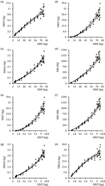
Generally, the time–implicit relationships of the growth patterns exhibited by the chemical constituents of the empty body were allometric to the estimated EBW and EBCP. Graphs built by plotting the composition of gain according to Eqns (20) and (21) revealed such relationships (Fig. 2). The behaviour of EBCF, EBAsh and EBE remained visually non-linear with respect to the estimated EBW (Fig. 2(b), (c) and (d)). The same can be said about observed and estimated 99%CI for EBCF, EBE and EBAsh plotted against the estimated EBCP (Fig. 2(e)–(g)). Because EBCP, EBH2O and EBW growth were best mimicked by Eqn (1) combined with Eqn (6) (Tables 1 and 2), an isometric growth might explain the profiles exhibited in panels a and h (Fig. 2). Therefore, it appears that EBH2O increased in an almost linear manner as the estimated EBCP increased, but showed an approachable asymptotic behaviour towards the larger protein amounts deposited in the empty body (Fig. 2(h)). If the respective estimates of the fractional growth rates of EBCP, EBH2O and EBW listed in Table 2 are taken as ratios on each other, for instance, 0·0017/0·0013 = 1·31 and 0·0028/0·0017 = 1·65, it can be seen that protein was deposited faster than EBW and water deposited faster than protein, respectively. The opposite behaviour was observed for EBCF, EBE and EBAsh, i.e., they were deposited faster only for larger estimated EBW values at late growth (Fig. 2).
Observed data (△) and point (solid lines) and 99% confidence interval (dashed lines) estimates for some variables plotted against the estimated empty body weight (EBW) and empty body crude protein (EBCP). On panels (a)–(d) are the respective plots of EBCP (kg), crude fat in the empty body (EBCF, kg), ash in the empty body (EBAsh, kg) and energy in the empty body (EBE, MJ) against EBW (kg). On panels (e)–(h) are the respective plots of EBCF, EBE, EBAsh and water in the empty body (EBH2O) against the EBCP.

Growth rates and composition of gain
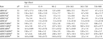
Time is explicit in ΔY t /Δt, but is implicit in ΔY t /ΔX t (Table 5). Therefore, based on the direct scaling relationship of Y t and X t , Eqn (22) combined with Eqn (8) was the best solution for scaling EBCP to both BW (Δ r = 0, w r = 0·897) and EBW (Δ r = 0, w r = 0·975), EBCF to both BW (Δ r = 0, w r ≅ 1·000) and EBW (Δ r = 0, w r ≅ 1·000), and EBE to both BW (Δ r = 1·7, w r = 0·303) and EBW (Δ r = 0, w r = 0·508). Equation (6) was equally as useful as Eqn (8) for describing the variability of EBE when scaled to BW (Δ r = 0, w r = 0·697) and EBW (Δ r = 0·1, w r = 0·492), but Eqn (8) was chosen, despite the fact that both shared the same value for Θ.
Estimates of the 99% confidence intervals (99%CI) presented as
 $\hat g(\hat \theta, \; t) \pm t_{\left( {1 - \alpha, \; \; df} \right)} SE_{\hat g(\hat \theta, \; t)} $
for the average daily rates of retention (ΔYt/Δt) of body weight (BW), empty body weight (EBW), crude protein (EBCP), crude fat (EBCF) and energy (EBE), and estimates of the 99%CI as
 $\hat g(\hat \theta, \; X_t ) \pm t_{\left( {1 - \alpha, \; \; df} \right)} SE_{\hat g(\hat \theta, \; X_t )} $
for EBCP, EBCF and EBE gains
 $(\Delta Y_t /\Delta X_t )$
for Xt = BW and Xt = EBW at specific age intervals

* df are degrees of freedom used to build the 99% confidence interval.
† g/day.
‡ MJ/day.
§ g/kg of gain.
¶ MJ/kg of gain.
DISCUSSION
Non-linear model selection
Many model combinations were used to quantitatively interpret the growth profiles of the present study, but only one model combination per variable was considered the best choice. These choices were based on a multi-model selection framework built on information-likelihood and additional criteria for selecting the model that best mimicked the data so that inferences on parameters and parameter functions could be made. Traditionally, some measures used to judge the quality of fit of different nested and non-nested models, such as the F-ratio and likelihood ratio tests, and R 2, are not effective and were neither used nor computed. In fact, F-ratios and likelihood-ratio tests introduce the dichotomy of rejecting or not rejecting the null hypothesis and do not provide a reasonable basis for multi-model selection (Burnham & Anderson Reference Burnham and Anderson2004; Stang et al. Reference Stang, Poole and Kuss2010). The R 2 or adjusted R 2 were inherited from linear models and their computation was not mentioned or said to be necessary according to specialized literature regarding non-linear models, e.g., Bard (Reference Bard1974), Ratkowsky (Reference Ratkowsky1990) and Pinheiro & Bates (Reference Pinheiro and Bates2000). Therefore, approaches that are more robust, such as information-likelihood criteria, are recommended (Spiess & Neumeyer Reference Spiess and Neumeyer2010). Provided that the sample is representative of the population, the AICc r (Akaike Reference Akaike1974; Sugiura Reference Sugiura1978) and its derived measures (Δ r , w r and ER r ) are rather informative (Burnham & Anderson Reference Burnham and Anderson2004).
Parameterization of growth models
The different growth patterns exhibited by the variables studied in the present paper motivated the investigation of the likelihood of not only the expected means, but also the likelihood of variance functions that may explain the observed heteroscedasticity of the growth profiles presented. The variance function
 $(\sigma _{Y_t} ^2 )$
complements the deterministic part of the non-linear model
 $(\mu _{Y_t} )$
, and both form the final stochastic version of the model, i.e.,
 $Y_t = \mu _{Y_t} + e_t $
for
 $Y_t \sim {\rm Normal}\,(\mu _{Y_t}, \sigma _{Y_t} ^2 )$
(Bard Reference Bard1974). There are some examples in the literature in which the covariance structures are modelled by accounting for a general increase in the variance over time (Pinheiro & Bates Reference Pinheiro and Bates2000; Littell et al.
Reference Littell, Milliken, Stroup, Wolfinger and Schabenberger2006; Strathe et al.
Reference Strathe, Danfaer, Sørensen and Kebreab2010; Vonesh Reference Vonesh2012). The method of maximum (and restricted maximum) likelihood estimates parameters and provides additional measures of the strength of evidence that the model mimics the real world (Pinheiro & Bates Reference Pinheiro and Bates2000; McCulloch & Searle Reference McCulloch and Searle2001; Vonesh Reference Vonesh2012). In the present study, for those variables in which a well-defined asymptotic phase was not evident, the exponential model, or Eqn (6), best mimicked the variability of the growth profiles and resulted in a better description of the variance increase over time. Some variables presented a distinguishable asymptotic phase, and this well-established attribute of the growth profile was most likely associated with a variance increase over time scaled by
 $\mu _{Y_t} $
and modelled as Eqn (8). However, a variance based on Eqn (8) can be said to be asymptotic only if the
 $\mathop {\lim} \limits_{t \to \infty} \mu _{Y_t} $
exists (Rocha et al.
Reference Rocha, Vieira, Abreu, Araujo, Glória, Tamy, Camisa Nova and Fernandes2015), which is not true for Eqn (9). The three patterns described by Eqns (6)–(8) are departures from the homoscedasticity assumption. Only experiments that last long enough to characterize maturity allow a proper estimation of the asymptotic weights and variability over time (Blaxter et al.
Reference Blaxter, Fowler and Gill1982; France et al.
Reference France, Dijkstra and Dhanoa1996; Strathe et al.
Reference Strathe, Danfaer, Sørensen and Kebreab2010). Otherwise, smaller time-trend effects jeopardise inferences regarding asymptotic estimates at maturity (Strathe et al.
Reference Strathe, Danfaer, Sørensen and Kebreab2010). The definition of the asymptotic growth phase is crucial to establish the weight and its variability at maturity, particularly for vertical production systems that host breeding categories such as replacement doelings, as is the case in some goat dairying systems (Morand-Fehr & Sauvant Reference Morand-fehr, Sauvant and Jarrige1988; Santos Júnior et al.
Reference Santos Júnior, Vieira, Henrique and Fernandes2008; Vieira et al.
Reference Vieira, Cabral, Souza, Fernandes, Henrique and Corte-Real2009).
The sexual condition (Strathe et al. Reference Strathe, Danfaer, Sørensen and Kebreab2010) and breed (Regadas Filho et al. Reference Regadas Filho, Tedeschi, Rodrigues, Brito and Oliveira2014) are additional determinant effects of growth trajectories. In the present study, the inclusion of the breed effect did not improve the information-likelihood of Eqn (1). If repeated measures had been taken for BW it would be possible to increase the degrees of freedom for finding significant effects of breed over parameters, as observed by Regadas Filho et al. (Reference Regadas Filho, Tedeschi, Rodrigues, Brito and Oliveira2014), but all other variables studied here (EBW, Carcass, AbFat, etc.) were measured by destructive methods and the elimination of the individual was inevitable. The lack of an adequate number of animals of both Swiss Alpine and Saanen breeds exerted a major influence on model fitting and the effect of breed did not improve the quality of fit of the models. Therefore, the inference space of the present study was constrained to the average body composition and composition of gain for animals irrespective of breed. Nonetheless, goats have not been grouped by breed or genotype to estimate nutrient requirements, but rather as belonging to functional breeding types, i.e., dairy, indigenous, or meat types, because effects other than functional type over protein and energy retention are harder to detect (Luo et al. Reference Luo, Goetsch, Nsahlai, Sahlu, Ferrell, Owens, Galyean, Moore and Johnson2004a , Reference Luo, Goetsch, Sahlu, Nsahlai, Johnson, Moore, Galyean, Owens and Ferrell b ; NRC 2007).
There are events and processes that may constrain the growing animal, such as weaning, puberty, maturation and seasonal variations in food availability and quality (Morand-Fehr Reference Morand-Fehr and Gall1981; Brunel et al. Reference Brunel, Ernande, Mollet and Rijnsdorp2013; Magistrelli et al. Reference Magistrelli, Aufy, Pinotti and Rosi2013; Marinho et al. Reference Marinho, Freitas, Falcão and Dias2013), which demand non-conventional approaches for the quantitative description of its growth. Therefore, multi-phasic non-linear models may be useful for interpreting growth profiles that present more than the one puberty inflection point, as the constraints to growth impinged by the environment may retard or accelerate the rate of weight gain outside the age of the point of inflection (Koops Reference Koops1986; Nešetřilová Reference Nešetřilová2005; Mendes et al. Reference Mendes, Muniz, Silva and Mazzini2008; Souza et al. Reference Souza, Carneiro, Malhado, Silva and Silveira2013; Rocha et al. Reference Rocha, Vieira, Abreu, Araujo, Glória, Tamy, Camisa Nova and Fernandes2015). However, the biphasic model or Eqn (4) did not supplant Eqn (1) in terms of likelihood criteria. Although puberty is not strictly applicable to wethers, puberty in specialized dairy goat breeds occurs between 90 and 120 days (Morand-Fehr Reference Morand-Fehr and Gall1981; Regadas Filho et al. Reference Regadas Filho, Tedeschi, Rodrigues, Brito and Oliveira2014) when the growth rate starts to decrease, and may be confounded with weaning effects due to the close proximity of these two events in time (Morand-Fehr Reference Morand-Fehr and Gall1981; Rocha et al. Reference Rocha, Vieira, Abreu, Araujo, Glória, Tamy, Camisa Nova and Fernandes2015).
Several post-natal growth profiles resembled the first-order monomolecular growth traditionally described by the law of diminishing returns, noted as the self-inhibiting growth phase by Brody (Reference Brody1945). This can be attributed to the fact that the inflection point might have occurred during the kid's pre-natal life. In fact, a Gompertz-like model has been applied to anticipate the growth of kids during pre-natal life to compute requirements for pregnancy (AFRC 1993; 1997). Therefore, the greater likelihood probability of Eqn (1) for describing BW (Table 1) may be a clear indication that the self-accelerating phase occurred during pre-natal growth and the self-inhibiting phase initiated near birth or soon after birth. The additional scaling parameter (n) of Eqn (3) did not increased the likelihood probability of this model, despite the flexible nature of Eqn (3) for describing monomolecular-like growth patterns (France et al. Reference France, Dijkstra and Dhanoa1996; López et al. Reference López, France, Gerrits, Dhanoa, Humphries and Dijkstra2000; Regadas Filho et al. Reference Regadas Filho, Tedeschi, Rodrigues, Brito and Oliveira2014).
The integrated sum of the growth rates of many body parts yields the growth pattern exhibited by the body as a whole (Owens et al.
Reference Owens, Dubeski and Hanson1993). As observed by France et al. (Reference France, Dijkstra and Dhanoa1996), there are growth rates that can be described empirically by first-order growth or dY/dt = k(Y
f
− Y) that originated Eqn (1), which was chosen to represent some growing body and body parts. Sigmoid models mimic growth profiles that may be the result of a gradual reduction of the fractional growth rate at birth, i.e., dY/dt = Ykexp( − Dt), that yields the Gompertz model, as described by Eqn (2). The general model built by Richards (Reference Richards1959) or Eqn (3) owes its general nature to fit monomolecular or sigmoid profiles due to the assumed growth rate,
 $dY/dt = kY(Y_f^n - Y^n )/(nY_f^n )$
, that generalizes the balance between catabolic and anabolic processes scaled to the body proper as suggested by von Bertalanffy (Reference von Bertalanffy1957). Biphasic models such as Eqn (4) can be introduced to address an asymptotic first-order growth combined with sigmoid growth so that
 $dY/dt = k_1 (Y_{f1} - Y) + Yk_2 \exp ( - Dt)$
; it is assumed that the first-order growth occurs primarily during the birth-weaning period and the sigmoid growth prevails after the weaning shock (Rocha et al.
Reference Rocha, Vieira, Abreu, Araujo, Glória, Tamy, Camisa Nova and Fernandes2015); therefore, the constraint k
2 < k
1 must hold. Rocha et al. (Reference Rocha, Vieira, Abreu, Araujo, Glória, Tamy, Camisa Nova and Fernandes2015) used a set of growing Saanen kids and a smaller subset of the present data, and found some influence of short-term effects and some likely existence of inflection points for growing kids until 200 and 365 days old. Because short-term effects have less influence on model fitting than a more complete time profile of animals growing to maturity (Strathe et al.
Reference Strathe, Danfaer, Sørensen and Kebreab2010), and for the sake of statistical rigour, Eqn (4) and its intrinsic assumptions were not likely to represent the long-term growth of the body, body parts and composition of gain of goat wethers.
The growing animal faces seasonal changes in the environment. If it grows with an unlimited food supply, growth is constrained mainly by genotype, and daily intake rate is expected to stabilize at maturity (Blaxter et al. Reference Blaxter, Fowler and Gill1982; Lawrence & Fowler Reference Lawrence and Fowler2002). Generally, after puberty, there are expenditures of nutrients for maintenance, somatic growth and reproduction (including lactation) that are balanced by the rate of nutrient intake (Brunel et al. Reference Brunel, Ernande, Mollet and Rijnsdorp2013). The growth condition is complex because a well-managed doe still grows after first kidding and reaches a steady-state mature size only after the second kidding (Morand-Fehr Reference Morand-Fehr and Gall1981). For castrated animals, a balance between nutrient acquisition and expense may explain growth stabilization (Blaxter et al. Reference Blaxter, Fowler and Gill1982), but the reproductive cycle constrains doelings and bucklings as they grow into adulthood. Blaxter et al. (Reference Blaxter, Fowler and Gill1982) theorized that maturity weight is achieved when energy intake and expenditure reach a balance because long-term intake at maturity and body composition reach a steady-state condition. This condition does not mean that maturity weight is immutable but rather is the balance between maintenance and reproductive expenditures, as well as efforts for harvesting nutrients from the environment (Lawrence & Fowler Reference Lawrence and Fowler2002).
From birth to mature empty body weights
The rate of fat deposition in does is larger than in wethers, which in turn is larger than in bucks; in addition, differences are more remarkable at heavier body weights (Mahgoub et al. Reference Mahgoub, Kadim, Al-Saqry and Al-Busaidi2004). Crossbreeds of Alpine × Hair and Saanen × Hair goats have heavier carcasses and internal fat weights than Hair breeds (Gökdal Reference Gökdal2013). Carmichael et al. (Reference Carmichael, Kouakou, Gelaye, Kannan, Lee and Terrill2012) argued that adult dairy goats (Saanen) most likely have more carcass fat than younger goats. By taking weights at 900 and 112 days from Table 4, the difference EBCF − AbFat was 14·7 and 1·3 kg of non-abdominal fat for adults and younglings, respectively.
The adipose tissue grows by both hypertrophic and hyperplasic mechanisms (Hossner Reference Hossner2005). Therefore, an unrestricted food supply may explain the absence of an asymptotic phase for the EBCF profile in Fig. 2(f), in which the predicted asymptote was twofold the predicted value at 900 days of age
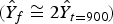 $(\hat Y_f \cong 2\hat Y_{t = 900} )$
. A corollary of this feeding regime is that as the growth rate of the animal increases, the accretion rate of fat increases and protein decreases (NRC 2007). This was confirmed by the results shown in Tables 3, 4, and 5; i.e., fat and protein contents in the empty body increase and decrease, respectively, as the wethers mature (Tedeschi et al.
Reference Tedeschi, Cannas and Fox2010). The 95%CIs for the average daily gain and for the average body weight of growing dairy animals reported by Luo et al. (Reference Luo, Goetsch, Sahlu, Nsahlai, Johnson, Moore, Galyean, Owens and Ferrell2004b
) were 0·14±0·014 kg/day and 23±1·5 kg, respectively. In the present study, animals of this size were 90–210 days old (Tables 3, 4 and 5). There is little information regarding body composition of goats (AFRC 1997; NRC 2007). Therefore, chemical composition estimates for the growing body of wethers obtained in the present study can be used ad interim to predict net energy and protein retention in the empty body of females for t < 210 days; for older ages, reproduction hampers generalizations.
The long-term profiles studied here by extending the EBW range from birth to maturity revealed a non-linear behaviour for body composition, although EBCP appeared to be isometric with respect to EBW, as well as water and protein shared an isometric growth in the EBW (Fig. 2). The body parts grew in an allometric manner as demonstrated by the existence of different ages at the detected points of inflection (Table 4), and by the observed different growth patterns and relationships (Figs 1 and 2). This allometric behaviour yielded different trends: some chemical constituents reached maturity earlier than others. This means that instant growth rates dY t /dX t for X t = EBW were not constant (the first derivative of Eqn (22) is not constant). Rather, Eqn (22) better described the relationship between EBW composition and EBW itself. Blaxter et al. (Reference Blaxter, Fowler and Gill1982) observed a linear increase for the lipid mass in the empty body of sheep, but they studied a heavier EBW range, i.e., from 46 to 130 kg, as the authors focused on the post-puberty phase of growth. The linear relationships for EBAsh and EBW observed in sheep by Blaxter et al. (Reference Blaxter, Fowler and Gill1982) do not appear to hold for goat wethers (Fig. 2(c)). Other relationships illustrated in Fig. 2 are curvilinear if compared with the linear growth behaviours reported by Blaxter et al. (Reference Blaxter, Fowler and Gill1982).
The linear mass accretions observed for Carcass, EBDM, EBAsh and EBE were not expected (Tables 1 and 2, and Fig. 1). The choices of Eqns (9), (6) and (8) were based on the criterion of full rank covariance matrix for parameters at convergence. The achievement of a positive definite Hessian is necessary for finishing the estimation procedure of a non-linear model by the nlme package of R (another statistical software system used to solve non-linear estimation problems: http://www.r-project.org/); otherwise, error messages are exhibited (Pinheiro & Bates Reference Pinheiro and Bates2000). The NLMIXED procedure output contains a covariance parameter matrix based on a Moore–Penrose inverse for the Hessian whenever the latter does not reach the ‘positive definiteness’ condition. A corollary of this scenario is that the Hessian is singular and some variance parameter estimates of the covariance matrix may be unreliable. Because interest here relied on inference, a more conservative criterion was adopted and models based on Δ r = 0 but without a full rank covariance matrix were disregarded from the solution set. The NLMIXED procedure, however, is based on the numerical integration of the likelihood function, which is maximized. If the convergence criterion is achieved, even with a singular Hessian, the point estimates of parameters are those that maximized the logarithm of the likelihood function (Littell et al. Reference Littell, Milliken, Stroup, Wolfinger and Schabenberger2006; Vonesh Reference Vonesh2012). Therefore, the models with Δ r = 0 were those with the highest adherence to the general growing tendencies exhibited by the data, despite the eventual output of unreliable standard errors for some parameters (not shown). This explains the choice of the best adherent model to estimate Eqn (12).
The linear EBE behaviour was the net result of the combined monomolecular growth of EBCP and the sigmoid growth of EBCF, as the sum of body parts forms the shape of the growth profile (Owens et al. Reference Owens, Dubeski and Hanson1993). The scaling function or Eqn (22), whose parameter estimates are not shown, was useful to estimate Eqn (23) as average rates of retention of protein, fat and energy in BW and EBW (Table 5). In summary, goat wethers of specialized dairy breeds grew from birth to maturity in an asymptotic, monomolecular time-trend for BW and EBW. However, body parts and chemical constituents of the body showed not only monomolecular growth, but also sigmoid and even linear growth trends as the animals aged. Some variables clearly presented well-defined asymptotic phases, but this was not true for all variables studied. The variances of the time-trends were both asymptotic and non-asymptotic, depending on the model chosen to represent variability and, ultimately, the existence of a well-defined asymptotic phase to the growth profile.
This research was supported by Conselho Nacional de Desenvolvimento Científico e Tecnológico – CNPq (Brazil), process numbers 306584/2012-3 and 479593/2010-8, and by Fundação Carlos Chagas Filho de Amparo à Pesquisa do Estado do Rio de Janeiro – FAPERJ (RJ, Brazil), process number E-26/110.231/2011. The first author thanks the fellowship provided by Coordenação de Aperfeiçoamento de Pessoal de Nível Superior (CAPES, Brazil) – Demanda Social Doutorado. We thank Professor Marcelo T. Rodrigues (DZO/UFV), who provided the animals. We thank the two anonymous reviewers whose contributions greatly enhanced the manuscript and proved that peer review is an essential part of the scientific publication process.