1. Introduction
Flapping-wing micro-air vehicles may suffer from a loss in the lifting surface owing to wing damage (Salem et al. Reference Salem, Cellini, Kabutz, Hari Prasad, Cheng, Jayaram and Mongeau2022). Assessing the aerodynamic effects of lifting-surface loss is a fundamental problem. Natural flyers with non-intact wings serve as ideal subjects for understanding the flow physics of lifting-surface loss (Lyu, Zhu & Sun Reference Lyu, Zhu and Sun2020; Rajabi, Dirks & Gorb Reference Rajabi, Dirks and Gorb2020; Hedenström Reference Hedenström2023). For example, birds periodically replace their flight feathers, mainly primary and secondary feathers, through a process known as moulting. The moulting process creates different trailing-edge gaps in their wings (Hedenström Reference Hedenström2023).
These trailing-edge moult gaps affects the aerodynamic performances of both gliding and flapping flight. During avian equilibrium gliding, sufficient lift is expected to attain a high lift-to-drag ratio for travelling a long horizontal distance. Tucker (Reference Tucker1991) experimentally measures the maximum lift-to-drag ratio of a Harris’s hawk during the moult duration at a given free stream velocity. A significant decrease in the maximum lift-to-drag ratio is observed after moult onset. This decrease reaches 31 % of the pre-moult level when the loss of the four primary feathers forms gaps in the wing tips. The reduction in the lifting surface accounts for 39 % of the observed decrease in the maximum lift-to-drag ratio according to equilibrium gliding performance theory (Tucker & Heine Reference Tucker and Heine1990). The remainder could be attributed to the changed spatial configuration of the wing tip slots. In addition, the efficiencies of the lift production for the available wing span and geometric angle of attack are measured using the span efficiency factor (Henningsson & Bomphrey Reference Henningsson and Bomphrey2013) and lift-curve slope, respectively. Hedenström & Sunada (Reference Hedenström and Sunada1999) model the wing geometry in three representative moult stages to numerically investigate the effects of one or two moult gaps of different sizes and positions on the span efficiency factor and lift-curve slope. The results show that the span efficiency factor and lift-curve slope decrease owing to the existence of a moult gap. The decrease in the lift-curve slope is almost independent of the gap width, whereas the decrease in the span efficiency factor is positively correlated with the gap width. For a moult gap with a width of 10 % that of the semi-span, the negative effects are most pronounced when the gap is located in the middle of the wing span, where the inner primary feathers or outer secondary feathers are missing. Nevertheless, the span efficiency factor and lift-curve slope gradually increase as the gap position moves towards the wing tip. As an exception, when the gap is near the wing tip, the lift distribution on the wing becomes approximately elliptical, which actually enhances the gliding performance. Furthermore, the experimental observations of KleinHeerenbrink & Hedenström (Reference KleinHeerenbrink and Hedenström2017) for a gliding jackdaw support the idea that the shedding of the inner primary feathers releases the constraints on the outer primary feathers, reducing the spanwise camber of the wing and thereby decreasing the span efficiency factor.
The negative effects of the moult gap on gliding aerodynamic performance can be alleviated using several methods. First, gliding birds adjust their wing morphology to minimise moult gaps (Tucker Reference Tucker1991; KleinHeerenbrink & Hedenström Reference KleinHeerenbrink and Hedenström2017). Second, increasing the geometric angle of attack narrows the disparity in gliding performance between the moult-gapped and intact wings (Sigrest & Inman Reference Sigrest and Inman2020). At the geometric angles of attack greater than 8
 $^\circ$
, the lift-to-drag ratio of the moult-gapped wing approaches that of the intact wing. Third, decreasing body weight, adopted by some birds, is beneficial for reducing the wing loading of moult-gapped wings (Senar, Domenech & Uribe Reference Senar2002; KleinHeerenbrink & Hedenström Reference KleinHeerenbrink and Hedenström2017). Based on the scaling of avian wings, the wing loading is proportional to the body weight raised to a power of
 $1/3$
(Liu Reference Liu2006; Sullivan, Meyers & Arzt Reference Sullivan, Meyers and Arzt2019). In addition, reducing the geometric aspect ratio decreases the reduction in the span efficiency factor of moult-gapped wings relative to intact wings (Hedenström & Sunada Reference Hedenström and Sunada1999).
As an alternative to gliding, flapping is a widely employed approach for hovering and forward flight. For hovering hummingbirds, a reduction in flight efficiency during moulting is observed by Chai (Reference Chai1997). He also emphasises that the loss of the lifting surface affects lift generation. In particular, reducing the area at the tip of the outer primary feathers leads to greater difficulties in producing sufficient lift compared with reducing the area of the inner secondary feathers. Flapping birds share similar responses to the possible performance deterioration with gliding birds (Chai Reference Chai1997; Tomotani & Muijres Reference Tomotani and Muijres2019). Songbirds with artificial moult gaps combine an increase in the geometric angle of attack with a reduction in the moult gap during vertical manoeuvring flight to obtain an unchanged net weight-normalised aerodynamic force (Tomotani & Muijres Reference Tomotani and Muijres2019).
Compared with gliding flight, flapping flight involves more complex vortex dynamics, which is closely related to the generation of aerodynamic forces (Wu, Lu & Zhuang Reference Wu, Lu and Zhuang2007; Li & Wu Reference Li and Wu2015; Liu, Wang & Liu Reference Liu, Wang and Liu2024). The flow is dominated by a vortex system composed of leading edge vortices (LEVs) (Videler, Stamhuis & Povel Reference Videler, Stamhuis and Povel2004; Maxworthy Reference Maxworthy2007; Muijres et al. Reference Muijres, Johansson, Barfield, Wolf, Spedding and Hedenstr̈m2008; Li et al. Reference Li, Feng, Kissing, Tropea and Wang2020), trailing edge vortices (TEVs) (Bomphrey et al. Reference Bomphrey, Nakata, Phillips and Walker2017; Liu, Du & Sun Reference Liu, Du and Sun2020; Corban, Bauerheim & Jardin Reference Corban, Bauerheim and Jardin2023) and tip vortices (TVs) (Birch & Lee Reference Birch and Lee2005; Shyy et al. Reference Shyy, Trizila, Kang and Aono2009; Zhang, Zhang & Huang Reference Zhang, Zhang and Huang2022). At the leading edge of the avian wing, the alula (or alular feather) forms a gap with the main wing at its root. This gap enhances the lift at post-stall angles of attack by inducing individual vortex structures that interact with the LEVs of the main wing (Linehan & Mohseni Reference Linehan and Mohseni2020). Similar aerodynamic benefits from gap flows dominated by vortex structures have been found in slotted wing tips (KleinHeerenbrink, Johansson & Hedenström Reference KleinHeerenbrink, Johansson and Hedenström2017), multi-feather configurations (Kim, Lee & Kim Reference Kim, Lee and Kim2019; Olivieri et al. Reference Olivieri, Boragno, Verzicco and Mazzino2019; Alben Reference Alben2021) and trailing-edge fringes (Rong & Liu Reference Rong and Liu2022; Deng, Yang & Chen Reference Deng, Yang and Chen2023). The enhancement of aerodynamic performance in these studies implies that the negative effect of the moult gap on flapping flight performance might be compensated by interactions among the vortices.
The moult gap of a wing can be considered a modification of the trailing-edge shape of the wing (Hedenström Reference Hedenström2023), which affects the formation and evolution of vortex structures around a flapping wing. The vortex dynamics of the flapping wing with smooth trailing edges has been investigated in previous studies (Von Ellenrieder et al. Reference Von, Karl, Parker and Soria2003; Trizila et al. Reference Trizila, Kang, Aono, Shyy and Visbal2011; Yilmaz & Rockwell Reference Yilmaz and Rockwell2012). Conversely, Van Buren et al. (Reference Van Buren, Floryan, Brunner, Senturk and Smits2017) focus on sharp changes in trailing-edge shape (symmetric chevron shape) and analyse the resulting performance of a pitching wing. It is found that a concave trailing edge suppresses the natural bending of TEVs and the compression of wake vortices, whereas a convex trailing edge promotes them. This change in the formation of TEVs is accompanied by the change in average wake velocity and correlates with differences in the average thrust and efficiency. Further work by Hemmati et al. (Reference Hemmati, Van Buren and Smits2019) identifies that the highest instantaneous thrust occurs simultaneously with the detachment of the TEVs. Zhang, Huang & Lu (Reference Zhang, Huang and Lu2020) also examine the influence of similar trailing-edge shapes on a heaving plate considering structural flexibility. The propulsion performance of the plate is caused by the distributions of the spanwise vorticity and the consequent jet momentum in the near wake. Another typical sharp change in the trailing-edge shape is the serrated trailing edge, which is found to weaken the TVs around a rectangular flat-plate wing during hovering flight (Ji et al. Reference Ji, Wang, Ravi, Tian, Young and Lai2022). These studies on concave/convex and serrated trailing edges indicate that changes in the entire trailing edge cannot be neglected in flapping flight. However, little is known about the effects of the moult gap on the aerodynamics of flapping flight.
The objective of this study is to investigate the effects of the moult gap on the aerodynamic performance and vortex dynamics in flapping flight. Moult gaps with different widths and positions are investigated by numerically solving the Navier–Stokes equations. The remainder of this paper is organised as follows. In § 2, we describe the bio-inspired model of a moult-gapped wing and a numerical method for solving the unsteady flow around the wing. An analysis of the effects of the moult gap on flapping aerodynamic performance is presented in § 3. Finally, the conclusions are given in § 4.
2. Numerical model and method
2.1. Moult-gapped wing model
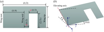
Schematic of the moult-gapped flapping wing. (a) Wing planform. (b) Wing kinematics described by the time-dependent elevation angle
 $\psi$
at a constant geometric angle of attack
 $\alpha$
. The
 $x$
,
 $y$
and
 $z$
axes of the global coordinate system are along the streamwise, spanwise and vertical directions, respectively.

The bio-inspired wing model with a trailing-edge moult gap is constructed according to Hedenström & Sunada (Reference Hedenström and Sunada1999), as shown in figure 1(a). A rectangular flat-plate wing with chord length
 $c$
and span length
 $b$
is adopted as the basic configuration. The geometrical aspect ratio
 $b/c$
of the original intact wing is 4 (Bhat et al. Reference Bhat, Zhao, Sheridan, Hourigan and Thompson2019). A rectangular gap is cut at the trailing edge to simulate the lifting-surface loss during moulting. The semi-span
 $b/2$
is used as the reference length because of the variable local chord length induced by the moult gap. The moult gap has a normalised length of
 $1/3$
and normalised width of
 $w$
to simulate the high ratio of the longitudinal to transverse sizes of actual flight feathers. The normalised gap position between the inner side edge of the gap and wing mid is
 $d$
. Table 1 presents the values of the normalised width and the normalised position of the moult gap in all the cases considered in this study. The interval for the normalised width of the moult gap is set at 0.05, which corresponds to the normalised width of a single flight feather (inner primary or outer secondary feather) based on the ratio of the feather barb width to the wing span (Tucker Reference Tucker1987; Feo, Field & Prum Reference Feo, Field and Prum2015). The geometrical aspect ratio of the moult-gapped wing is larger than that of the intact wing owing to the reduced wing area. The moult-gapped wing operates in a fluid with density
 $\rho$
and kinematic viscosity
 $\nu$
and experiences a uniform incoming flow with velocity
 $U_{\infty }$
.
Set-up of the geometrical parameters of the intact and moult-gapped wings.

The kinematics of the moult-gapped wing is given by a time-dependent elevating motion at a constant geometric angle of attack. In figure 1(b), we define a global coordinate system
 $o{-}xyz$
with origin
 $o$
at the trailing-edge point of the wing root line and the
 $x$
,
 $y$
and
 $z$
axes along the streamwise, spanwise and vertical directions, respectively. The moult-gapped wing is tilted about the global
 $y$
axis to a geometric angle of attack
 $\alpha$
of 25
 $^\circ$
, around which the net weight-normalised aerodynamic force is effectively compensated (Tomotani & Muijres Reference Tomotani and Muijres2019). This geometric angle of attack is aligned with the stroke plane angle commonly used by flying animals (Tobalske & Dial Reference Tobalske and Dial1996; Wolf et al. Reference Wolf, Johansson, von Busse, Winter and Hedenström2010). At this geometric angle of attack, the moult-gapped wing revolves around the wing root line (shoulder joint), which is described by an elevating angle
 $\psi$
(Parslew Reference Parslew2015; Baliga, Szabo & Altshuler Reference Baliga, Szabo and Altshuler2019), as illustrated in figure 1(b). The change in the elevation angle
 $\psi$
with dimensionless time
 $t$
is specified in the following simple harmonic form (Lua et al. Reference Lua, Lee, Lim and Yeo2016):
 \begin{equation} \psi (t)={\psi }_{0}+{\psi }_{m} \sin (2{\pi }ft), \end{equation}
where
 ${\psi }_{0}$
is the mean elevation angle,
 ${\psi }_{m}$
is the elevation amplitude and
 $f$
is the dimensionless elevation frequency normalised by the reference frequency
 ${2{U}_{\infty }}/{b}$
. In this context, elevation aligns with the upstroke, whereas depression matches with the downstroke. The kinematical parameters derived from the actual flapping wing motion, as detailed by Liu et al. (Reference Liu, Kuykendoll, Rhew and Jones2006) and Wang et al. (Reference Wang, Liu, Xu and Wang2022), are listed in table 2. Two groups of moult-gapped wings are considered in this study, that is, GWA1–6 and GWB1–8, as presented in table 1, which are employed to investigate the effects of gap width and gap position, respectively, on the aerodynamic performance of the moult-gapped wing. To elucidate the role of the moult gap, an intact wing (IW) in table 1, characterised by the same elevation kinematical parameters, is also included in the present cases.
Set-up of the kinematical parameters of the intact and moult-gapped wings.

2.2. Methods and set-ups
The three-dimensional incompressible viscous flow encompassing the moult-gapped wing is described by the corresponding Navier–Stokes equations. In the framework of the immersed boundary method adopted in this study, the equations can be written as follows:
 \begin{equation} \boldsymbol{\nabla }\boldsymbol{\cdot }\boldsymbol{u}=0, \end{equation}
 \begin{equation} \frac {\partial \boldsymbol{u}}{\partial t} + \boldsymbol{u} \boldsymbol{\cdot }\boldsymbol{\nabla }\boldsymbol{u} = -\boldsymbol{\nabla }p + \frac {1}{{\textit{Re}}} {{{\nabla} }^{2}}\boldsymbol{u} + {{\boldsymbol{f}}^{*}}, \end{equation}
where
 $\boldsymbol{u}$
denotes the dimensionless velocity vector normalised by the free stream velocity
 ${U}_{\infty }$
and
 $p$
is the dimensionless pressure normalised by
 $\rho U_{\infty }^{2}$
. The Reynolds number is defined based on the radius of gyration
 $r_g$
of the wing model, that is,
 ${\textit{Re}}={{{U}_{\infty }}r_g}/{\nu }$
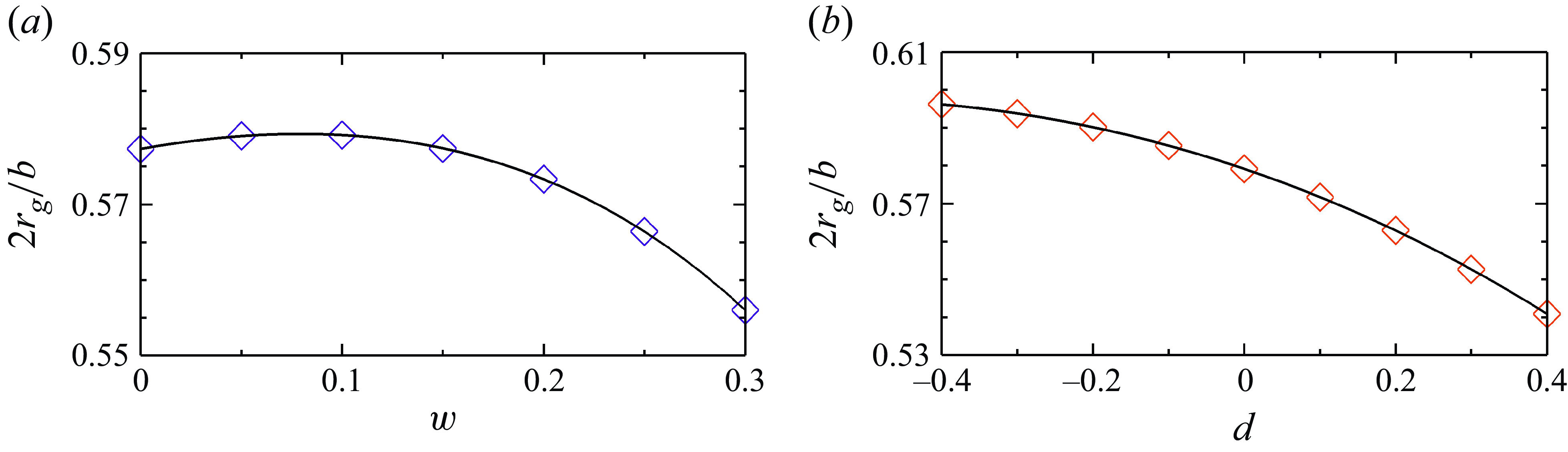
. The radius of gyration reflects the distribution of the lifting-surface area relative to the elevating axis. The normalised radius of gyration under all cases is plotted in figure 2. The Reynolds number of the intact wing is set to 346, considering the balance between ensuring adequate grid resolution and capturing the unsteady vortex dynamics according to the similar simulations in the literature (Shyy et al. Reference Shyy, Trizila, Kang and Aono2009; Taira & Colonius Reference Taira and Colonius2009; Medina et al. Reference Medina, Eldredge, Kweon and Choi2015; Kim et al. Reference Kim, Lee and Kim2019; Bhat et al. Reference Bhat, Zhao, Sheridan, Hourigan and Thompson2020). This is based on the assumption that the separation point of the flow over a flapping wing with a sharp leading edge is not sensitive to the Reynolds number, and that the unsteady flow is dominated by the Strouhal number (Ho et al. Reference Ho, Nassef, Pornsinsirirak, Tai and Ho2003; Buchholz & Smits Reference Buchholz and Smits2006). The effects of the Reynolds number are examined in Appendix A. The body force
 ${\boldsymbol{f}}^{*}$
is used in the immersed boundary method to represent the effect of the flapping wing on the fluid.
Normalised radius of gyration
 $2r_g/b$
. (a) Dependence on the normalised gap width
 $w$
for a fixed normalised gap position (
 $d=0$
). (b) Dependence on the normalised gap position
 $d$
for a fixed normalised gap width (
 $w=0.1$
).

We use the immersed boundary method in a discrete stream function formulation to solve the Navier–Stokes equations numerically. The second-order finite volume method is used for spatial discretisation, and the three-step, second-order and low-memory Runge–Kutta scheme is used for time advancement. Through precise projection methods, the condition of no divergence is ensured to the machine zero. In the momentum equation, the convection term is discretised explicitly and the diffusion term is treated implicitly. The details of the numerical method can be found in our previous work (Wang & Zhang Reference Wang and Zhang2011; Wang et al. Reference Wang, He and Zhang2013a ).
The computational domain is a cuboid with the coordinate ranges in the streamwise, spanwise and vertical directions of
 $[-2,4]b$
,
 $[-3,3]b$
and
 $[-5/2,5/2]b$
, respectively. The background mesh covers the computational domain, with
 $b/80$
as the minimum grid width in the near field and
 $b/20$
as the maximum grid width in the far field to ensure computational efficiency. The average size of the mesh representing the flapping wing is
 $b/80$
to guarantee the interpolation accuracy of the velocity
 $\boldsymbol{u}$
and external force
 ${\boldsymbol{f}}^{*}$
between the background and wing meshes. Free incoming and free convection conditions are specified at the inlet and outlet of the square computational domain, respectively. At the remaining four side boundaries, free-slip conditions are assigned. No-slip velocity is satisfied on the wall of the moult-gapped flapping wing. At the initial moment of the simulation, a unit flow velocity pervades the entire flow region. The simulation time is sufficiently long to ensure that the effect of the start-up process on the flow is negligible (as measured by the periodicity of the force coefficient). The aforementioned numerical settings have been used in several examples of flapping wing motion (Wang et al. Reference Wang, Xu, Zhang and Wang2021, Reference Wang, Liu, Xu and Wang2022). The detailed validations of the numerical method and checks of the grid independence can be found in our previous work (Wang et al. Reference Wang, Zhang, He and Liu2013b
, Reference Wang, He and Zhang2015a
,
Reference Wang, Zhang, He and Liub
, Reference Wang, He and Liu2019; Zhang et al. Reference Zhang, He, Wang and Zhang2019; Tong, Yang & Wang Reference Tong, Yang and Wang2021).
Panel (a) Computational domain showing the grid distribution around the moult-gapped wing. The boundary conditions are also marked on the corresponding surfaces. Panel (b) includes the wing mesh and background mesh extracted from the horizontal plane
 $z=0$
.

Two types of aerodynamic force coefficients are used in accordance with different reference areas. To compare the total aerodynamic forces, we choose a nominal area as follows as a reference area:
 \begin{equation} {S_n}=\frac {{b}{c}}{2}, \end{equation}
which is the area of a single intact wing. The corresponding force coefficients are denoted by the subscript
 $n$
. This type of force coefficient is hereafter referred to as the nominal aerodynamic force coefficient. The nominal lift and drag coefficients of the flapping wing are calculated as follows:
 \begin{equation} {{C}_{L,n}}=\frac {{{F}_{z}}}{{1}/{2}\;\rho U_{\infty }^{2}S_n}, \quad {{C}_{D,n}}=\frac {{{F}_{x}}}{{1}/{2}\;\rho U_{\infty }^{2}S_n}, \end{equation}
where
 ${F}_{z}$
and
 ${F}_{x}$
are the vertical and streamwise integrated fluid forces in the global coordinate system
 $o{-}xyz$
, respectively. To compare the aerodynamic forces per unit area, we choose the actual area of the single wing,
 \begin{equation} {S_a}=\frac {{b}{c}}{6}(3-2{w}), \end{equation}
as the reference area. The corresponding force coefficients are distinguished by the subscript
 $a$
. We hereafter designate this particular type of force coefficient as the actual aerodynamic force coefficient. Under these conditions, the expressions for the actual lift and drag coefficients of the flapping wing are
 \begin{equation} {{C}_{L,a}}=\frac {{{F}_{z}}}{{1}/{2}\;\rho U_{\infty }^{2}S_a}, \quad {{C}_{D,a}}=\frac {{{F}_{x}}}{{1}/{2}\;\rho U_{\infty }^{2}S_a}. \end{equation}
Using the instantaneous force coefficient, the period-averaged force coefficient (denoted by the overline) is computed as follows:
 \begin{equation} \overline { {C}_{\left \langle \centerdot \right \rangle } } = \frac {1}{T} \int _{T}{ {{C}_{\left \langle \centerdot \right \rangle }} (t) \,{\rm d}t}, \end{equation}
where
 $T=1/f$
is the dimensionless period of elevation motion.
3. Results and discussion
3.1. Effect of gap width on aerodynamic forces
Effect of gap width on average nominal aerodynamic force coefficients. (a) Average nominal lift coefficient
 $\overline {{C}_{L,n}}$
. (b) Average nominal lift-to-drag ratio
 ${\overline {{C}_{L,n}}}/{\overline {{C}_{D,n}}}$
. The solid line denotes the results of the present unsteady simulation, the dashed line corresponds to the results of the quasi-2-D model, where the aerodynamic force is proportional to the lifting-surface area and the dash–dotted line reflects the results of the quasi-steady lift model of Nabawy & Crowther (Reference Nabawy and Crowther2014b
). The case of
 $w=0$
corresponds to the intact wing.

Figure 4 illustrates the effect of gap width on the average nominal aerodynamic force coefficients. The solid line with triangular symbols represents the results of the present numerical simulation. The moult-gapped wing with a normalised gap width
 $w \leqslant 0.1$
almost maintains the average nominal lift coefficient
 $\overline {{C}_{L,n}}$
, which is equivalent to that of the intact wing. As the normalised gap width
 $w$
increases to 0.2 and 0.3, the average nominal lift coefficient
 $\overline {{C}_{L,n}}$
of the moult-gapped wing decreases to 0.71 and 0.63, respectively. To identify the factors that affect the aerodynamics of the moult-gapped wing, we introduce the results based on two theoretical models in figure 4. The dashed line with circular symbols is derived from the quasi-two-dimensional (quasi-2-D) model, which assumes that the aerodynamic force is proportional to the lifting-surface area. The cases denoted by the dashed line employ the same aerodynamic forces per unit area as those of the intact wing. In addition, the dash–dotted line with square symbols in figure 4(a) represents the predicted results of the quasi-steady lift model for general intact flapping wings. This quasi-steady lift model is proposed by Nabawy & Crowther (Reference Nabawy and Crowther2014b
), and includes both translational and non-translational components. The non-translational components are equal to zero, since the flapping wing in this work does not rotate about its spanwise axis during stroke reversal, and the elevation motion is symmetric between the upstroke and downstroke. The translational component dominates the generation of average lift and is expressed as the function of the geometric angle of attack
 $\alpha$
as
 \begin{equation} (\overline {C_{L,a}})^{ \textit{quasi-st.}}=\frac {{{{\kappa }_{ {2D}}}}/{2}} {E+{{{\kappa }_{ {2D}}}}/({\pi {e}{{AR}_{a}}})}\sin \left ( 2\alpha \right ), \end{equation}
where
 $\kappa _{ {2D}}$
is the lift-curve slope of a two-dimensional flat-plate aerofoil, which is set to
 $5.16$
to account for the effect of the Reynolds number (Okamoto, Yasuda & Azuma Reference Okamoto, Yasuda and Azuma1996). The geometry-specific parameter
 $E$
is the Jones edge velocity correction for the variation in the local chord of finite span wing (Jones Reference Jones1941). The Jones edge velocity correction is defined as the ratio of the wing semi-perimeter to the wing span, which is
 $3/2$
and
 $11/6$
for the intact and moult-gapped wings, respectively. Here,
 ${AR}_{a}$
is the actual aspect ratio of a single wing, which is given by
 ${{b}^2}/4{S_a}$
. The span efficiency factor
 $e$
corresponds to the induced angle of attack due to the finite span (Dommasch, Sherby & Connolly Reference Dommasch, Sherby and Connolly1961). This span efficiency factor is 0.75, which is close to the mean value evaluated by Muijres et al. (Reference Muijres, Spedding, Winter and Hedenström2011, Reference Muijres, Bowlin, Johansson and Hedenström2012) and Nabawy & Crowther (Reference Nabawy and Crowther2014a
) for flapping flight. The nominal lift coefficient predictions of this formula are obtained through a reference area conversion.
The intact wing is represented in figure 4 by a normalised gap width
 $w=0$
to clarify the effect of the moult gap. The average nominal lift coefficient
 $\overline {{C}_{L,n}}$
(a measure of the total aerodynamic force) of the intact wing is 0.76, which agrees well with that of the quasi-steady lift model. The average nominal lift coefficient
 $\overline {{C}_{L,n}}$
of the moult-gapped wing does not exceed that of the intact wing owing to the loss of the lifting surface. For these moult-gapped wings, the average nominal lift coefficient
 $\overline {{C}_{L,n}}$
almost decreases with an increase in the gap width.
The average nominal lift coefficient has the slowest decline rate relative to the normalised gap width when compared with the results from the quasi-2-D and quasi-steady lift models. The quasi-2-D lift model exhibits a linear decrease induced solely by the reduction in the lifting-surface area, whereas the quasi-steady lift model presents a more rapid decrease owing to the finite wing span. This comparison suggests that the loss of the lifting surface not only reduces the area supporting the aerodynamic loading, but also triggers a nonlinear flow mechanism. The nonlinear flow mechanism mitigates the reduction in aerodynamic force caused by the moult gap.
Despite its benefits, this nonlinear flow mechanism cannot prevent a decrease in the average lift-to-drag ratio of the moult-gapped wings, as shown in figure 4(b). The average nominal lift-to-drag ratio
 ${\overline {{C}_{L,n}}}/{\overline {{C}_{D,n}}}$
of the intact wing is 1.45. The moult-gapped wing with a normalised gap width of
 $w=0.1$
has an average nominal lift-to-drag ratio
 ${\overline {{C}_{L,n}}}/{\overline {{C}_{D,n}}}$
of 1.41, which is 3 % smaller than that of the intact wing. This results from an increase in the average nominal drag coefficient
 $\overline {{C}_{D,n}}$
that occurs during the early stages of moulting in the investigation of gliding flight (KleinHeerenbrink & Hedenström Reference KleinHeerenbrink and Hedenström2017). As the gap width increases, the effect of the reduction in the lifting-surface area is revealed. When the normalised gap width reaches 0.15, the average nominal lift-to-drag ratio
 ${\overline {{C}_{L,n}}}/{\overline {{C}_{D,n}}}$
is close to the value of the intact wing owing to the almost identical average nominal drag coefficient
 $\overline {{C}_{D,n}}$
. This almost-identity results from the cancellation between the reduction in the lifting-surface area and the increase in the drag per unit area. For the wide gaps (
 $w=0.2$
and
 $w=0.3$
), the decrease in the average nominal lift-to-drag ratio
 ${\overline {{C}_{L,n}}}/{\overline {{C}_{D,n}}}$
is attributed to the larger decrease in the average nominal lift coefficient
 $\overline {{C}_{L,n}}$
compared with that in the average nominal drag coefficient
 $\overline {{C}_{D,n}}$
. As observed by Sunada et al. (Reference Sunada, Takashima, Hattori, Yasuda and Kawachi2002) and Lee & Kim (Reference Lee and Kim2017), the average nominal lift coefficient
 $\overline {{C}_{L,n}}$
decreases more rapidly than the average nominal drag coefficient
 $\overline {{C}_{D,n}}$
under wide gaps, which Lee & Kim (Reference Lee and Kim2017) ascribed to the higher sensitivity of lift compared with drag to changes in the wing shape.
Effect of gap width on average actual lift coefficient
 $\overline {{C}_{L,a}}$
. The legends are the same as those in figure 4. The case of
 $w=0$
corresponds to the intact wing.

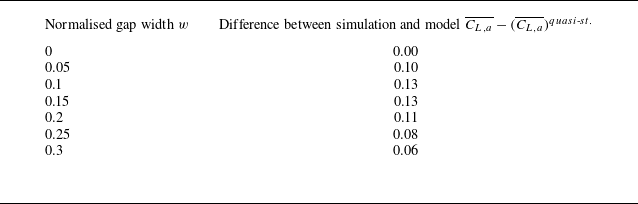
The actual aerodynamic coefficient reflects the relative magnitude of the decrease in the aerodynamic force and reduction in area. Figure 5 shows the average actual lift coefficients of the intact and moult-gapped wings. Because the proportion of lifting-surface reduction is larger than that of aerodynamic lift reduction, the average actual lift coefficients of the moult-gapped wing are greater than those of the intact wing. Larger average actual aerodynamic force coefficients of the moult-gapped wing were also observed in experimental measurements of hovering hummingbirds by Chai (Reference Chai1997). Among these moult-gapped wings, those with normalised gap widths of 0.1 and 0.2 exhibit equal reduction proportions in average lift and area, resulting in an equal average actual lift coefficient of 0.82. When the normalised gap width increases to 0.3, the average actual lift coefficient decreases to 0.79. The average actual lift-to-drag ratio
 ${\overline {{C}_{L,a}}}/{\overline {{C}_{D,a}}}$
exactly equals the average nominal lift-to-drag ratio
 ${\overline {{C}_{L,n}}}/{\overline {{C}_{D,n}}}$
because the difference between them lies only in the reference area. The quasi-steady lift model cannot accurately detect unsteady interactions caused by moult gaps, resulting in an underestimation of the average actual lift coefficient. Table 3 shows the difference in the average actual lift coefficient between the results of the present unsteady simulation and quasi-steady lift model. The quasi-steady lift model underestimates by up to 16 % compared with the numerical simulation when the gap width is 0.1. Even for the moult-gapped wing with the gap width of 0.3, which has the smallest underestimation by the model, the difference in average actual lift coefficient is still 8 %.
Difference in the average actual lift coefficient between the unsteady simulation and quasi-steady model of Nabawy & Crowther (Reference Nabawy and Crowther2014b ).

To investigate the change in the average nominal aerodynamic force coefficients, the histories of the instantaneous nominal aerodynamic coefficients of the moult-gapped wings with different gap widths during the flapping period are plotted in figure 6. The white and shaded blocks represent the upstroke and downstroke of the flapping wing, respectively. When the normalised gap width
 $w$
is 0.1, during the downstroke, the curves of the nominal lift coefficient
 ${C}_{L,n}$
and nominal drag coefficient
 ${C}_{D,n}$
of the moult-gapped wing are slightly different from those of the intact wing. This slight difference shows that the moult-gapped wing with a normalised gap width
 $w$
of 0.1 does not suffer a significant loss in aerodynamic force owing to the lifting surface reduction. As the gap width increases (the normalised gap width
 $w$
increases to 0.2 and 0.3), the instantaneous lift and drag gradually decrease. As shown in figure 6, the maximum decrease in the aerodynamic force owing to the lifting-surface loss occurs near the peak of aerodynamic force during the downstroke. Near the moment of maximum aerodynamic force, the decrease in the force is faster than the decrease in the area for wide gaps. At the moment of
 $t/T=3.45$
, for normalised gap widths
 $w$
of 0, 0.1, 0.2 and 0.3, the ratio of the nominal lift coefficients is
 $1:0.96:0.85:0.73$
, whereas the ratio of the actual lifting-surface areas is
 $1:0.93:0.87:0.80$
. Conversely, the further away from the moment of maximum aerodynamic force, the weaker the effect of area loss. During the upstroke, the aerodynamic forces of the wings with different gap widths tend to be consistent. The moult gap enhances the aerodynamic force relative to the intact wing during part of the upstroke (see the time intervals
 $3.00\lt t/T\lt 3.10$
and
 $3.90\lt t/T\lt 4.00$
in figure 6).
Effect of the gap width on the total aerodynamic forces of the moult-gapped wing. (a) Nominal lift coefficient
 ${C}_{L,n}$
. (b) Nominal drag coefficient
 ${C}_{D,n}$
. The subscript
 $n$
indicates that the reference area is the area of the intact wing. The white and shaded blocks represent the upstroke and downstroke of the flapping wing, respectively.

The larger average actual lift coefficient of the moult-gapped wing compared with the intact one is a consequence of temporal accumulation, as shown in figure 7. To facilitate comparison, the differences in the aerodynamic coefficients between the moult-gapped and intact wings are also plotted. The positive increment in the instantaneous actual lift coefficient
 ${C}_{L,a}$
of the moult-gapped wing persists for most of the flapping period, although the positive increment is small. The moult-gapped wing only exhibits a lower actual lift coefficient
 ${C}_{L,a}$
during the time interval
 $3.70 \lt t/T \lt 3.86$
when the normalised gap width
 $w$
is 0.1, and during the acceleration stage
 $3.25 \lt t/T \lt 3.50$
of the downstroke when the normalised gap width
 $w$
is 0.2 and 0.3. The actual lift coefficient curve of the moult-gapped wing, with a normalised gap width of 0.3, decreases more near the peak. It is worth noting that despite the different gap sizes, the actual drag coefficient
 ${C}_{D,a}$
of the moult-gapped wing is always greater than that of the intact wing. During most of the upstroke, the actual drag coefficient
 ${C}_{D,a}$
increases monotonically as the gap widens. When these results are considered alongside the experimental data from KleinHeerenbrink & Hedenström (Reference KleinHeerenbrink and Hedenström2017), it is plausible that increased drag is a common feature that is consistent in both gliding and flapping flight modes.
Effect of the gap width on the aerodynamic forces per unit area of the moult-gapped wing. (a) Actual lift coefficient
 ${C}_{L,a}$
. (b) Actual drag coefficient
 ${C}_{D,a}$
. (c) Difference in the actual lift coefficient
 ${\Delta }{C}_{L,a}$
. (d) Difference in the actual drag coefficient
 ${\Delta }{C}_{D,a}$
. The subscript
 $a$
indicates that the reference area is the area of the actual wing. The white and shaded blocks represent the upstroke and downstroke of the flapping wing, respectively.

3.2. Vortex dynamics of moult-gapped wings
The above-mentioned analysis of the aerodynamic forces of moult-gapped wings with different gap widths shows that the moult-gapped wing can generate more aerodynamic force per unit area. To reveal the vortex dynamics associated with these changes, the vortices of the intact and moult-gapped wings are compared in this subsection.
Figure 8 shows the vortices of the intact wing and the moult-gapped wing with a normalised gap width
 $w$
of 0.2 at three equally spaced moments during the upstroke deceleration stage (
 $3.00\lt t/T\lt 3.25$
). These vortices are identified using isosurfaces of the
 $Q$
-criterion (Hunt, Wray & Moin Reference Hunt, Wray and Moin1988) and coloured by the spanwise vorticity. For the intact wing, the LEVs appear along the entire span of the wing with their streamwise size increasing continuously, as the flapping velocity of the moult-gapped wing gradually decreases to zero, as shown in figure 8(a). Simultaneously, the TEVs are convected towards the wake. The TVs swing from the lower side to the upper side relative to the wing plane.
The flow over the moult-gapped wing contains vortices with similar characteristics. However, the moult gap at the trailing edge induces distinct local vortices. The most important feature is that the shear layer at the edges of the moult gap develops into a type of attached vortex structures. We refer to these vortex structures as gap vortices (GVs), according to the work of Lee, Lahooti & Kim (Reference Lee, Lahooti and Kim2018). To illustrate the features of GVs, figure 9(a) presents an isosurface with the
 $Q$
-criterion of 5 to depict the three-dimensional structure of GVs around the moult-gapped wing with a normalised gap width
 $w$
of 0.2. The GVs are composed of three segments attached to the inner, leading and outer edges of the moult gap. The GVs use their inner and outer edge segments to connect the TEVs of the moult-gapped wing. As shown in figure 9(b), the inner and outer edge segments are a pair of counter-rotating streamwise vortices with comparative strengths. The magnitude of this pair of vortices is larger at the mid-chord position of the moult gap than at both ends.
Vortices in the flow over the intact and moult-gapped wings during the upstroke deceleration stage (
 $3.00\lt t/T\lt 3.25$
). (a) Intact wing. (b) Moult-gapped wing (the normalised gap width
 ${w}=0.2$
). Free stream flow is directed from left to right. The vortex structures are represented by isosurfaces of
 $Q=3$
and coloured by the normalised spanwise vorticity
 ${\omega }_{y}$
.

Gap vortices (GVs) around the moult-gapped wing. (a) Spacial structure. (b) Normalised streamwise vorticity in the inner (
 $\triangle$
) and outer (
 $\square$
) edge segments. The plot shows the attached vortex structures of the moult-gapped wing with a normalised gap width
 $w$
of 0.2 at the moment
 $t/T=3.30$
. The vortex structures are represented by isosurfaces of
 $Q=5$
in panel (a). The normalised streamwise vorticity
 ${\omega }_{x}$
is displayed in four slices at normalised streamwise positions of –0.1, 0, 0.1 and 0.2 in panel (b).

Vortices in the flow over the intact and moult-gapped wings during the downstroke. (a) Intact wing. (b) Moult-gapped wing (the normalised gap width
 ${w}=0.2$
). Free stream flow is directed from left to right. The vortex structures are represented by isosurfaces of
 $Q=3$
and coloured by the normalised spanwise vorticity
 ${\omega }_{y}$
.

Normalised spanwise vorticity in the flow over the intact and moult-gapped wings during the downstroke. (a) Intact wing. (b) Moult-gapped wing (the normalised gap width
 ${w}=0.2$
). Free stream flow is directed from left to right. The spanwise distance from the slice to the symmetry plane at the wing root is 56 % of the semi-span. The slice crosses the narrow section with the moult gap.

When the intact wing and the moult-gapped wing with a normalised gap width
 $w$
of 0.2 enter the downstroke, the respective vortex structures at four equally spaced moments (the moment
 ${t}/{T}=3.76$
represents the end of the downstroke) are shown in figure 10. To elucidate the effects of the moult gap, figure 11 presents the distribution of spanwise vorticity
 ${\omega }_{y}$
in a slice located 56 % of the semi-span from the symmetry plane at the wing root. The slice passes through narrow sections of the moult-gapped wing with a normalised gap width
 $w$
of 0.2 throughout the downstroke. Before the mid-downstroke
 ${t}/{T}=3.50$
, the streamwise size of the LEVs over the intact wing continues to increase and gradually evolves to a spiral configuration, as observed in figures 10(a) and 11(a). The TEVs of the intact wing are convected downstream during the downstroke acceleration stage (
 $3.25\lt t/T\lt 3.50$
). The TEVs shed in the form of a single semi-ring together with the TVs at the moment
 ${t}/{T}=3.63$
in the following deceleration stage.
For the moult-gapped wing, the streamwise development of the LEVs produces their interaction with the GVs, resulting in a reduction in the streamwise size of LEVs compared with that of the intact wing (at the moment
 ${t}/{T}=3.37$
). The interaction between the LEVs and GVs also changes the spanwise distribution and shedding process of the LEVs, as shown in the three windows in figure 10(b). Furthermore, the moult gap changes the evolution of the TEVs, leading to the TEVs shedding in the form of double semi-rings at the moment
 ${t}/{T}=3.63$
. This is because of the simultaneous shedding of the inner and outer edge segments of the GVs and their connected TEVs.
The flow at the moult gap is characterised by the appearance of the GVs. The evolution of GVs remains consistent as the gap width varies. The GVs are responsible for aerodynamic compensation for the lifting-surface loss of the moult-gapped wings. The GVs induce nonlinear interactions among the vortices generated in the flapping flight. The GVs affect the evolution of other main vortex structures, thereby altering the vortex lift. At the same time, the GVs adjust the gap leakage flow, which modifies the near wake by changing the flow momentum (detailed in § 3.3). The moult-gapped wing relies on these interactions to compensate for the lost aerodynamic force, which is identified as vortex compensation. This vortex compensation corrects the discrepancy between the results (
 $\overline {C_{L,a}}$
) of the unsteady simulation and the predictions (
 $(\overline {C_{L,a}})^{ {quasi\text{-}st.}}$
) of the quasi-steady lift model (3.1) by
 \begin{equation} \overline {C_{L,a}}=(\overline {C_{L,a}})^{ \textit{quasi-st.}}+(\overline {C_{L,a}})^{ {\textit{gap}}}, \end{equation}
where
 $(\overline {C_{L,a}})^{ {\textit{gap}}}$
is the contribution of the vortex compensation.
The vortices around the flapping wing can be modelled as a vortex loop (Hedenström et al. Reference Hedenstr̈m, Johansson, Wolf, von Busse, Winter and Spedding2007). The change in the vortex loop from the intact wing to the moult-gapped wing is displayed in figure 12. This change affects unsteady lift, thereby modifying average lift (Wang & Wu Reference Wang and Wu2010; Chowdhury & Ringuette Reference Chowdhury and Ringuette2019). The correlation between the vortex loops and the average lift can be described by an actuator disk model (Spalart Reference Spalart2003; Oh et al. Reference Oh, Lee, Park, Choi and Kim2020). To compute the average lift of flapping wings in forward flight, Muijres et al. (Reference Muijres, Spedding, Winter and Hedenström2011) have modified the actuator disk model, which involves the unsteady vortex dynamics by using the non-uniform vertical induced velocity and the modified actuator disk area. The modified actuator disk area is selected as the area enclosed by the main vortex structures developed within one flapping period. The average lift is the change rate of downward momentum across the control surface around the flapping wing. The downwash flow at the actuator disk is visualised in figure 12(a).
Schematic of the vortex loops formed by the main vortex structures. (a) Intact wing. (b) Moult-gapped wing. The dashed lines represent the vortex lines, with thin arrows indicating their directions. The bold arrows denote the downwash flow at the modelled actuator disk. An observation slice is visualised in panel (b).

Generation of the increased induced downwash at the double vortex loops. The schematic is plotted on the observation slice in figure 12. The upward gap leakage through the moult gap creates the GVs, which increase the induced downwash. The variables
 $r_{ {\textit{in}}}$
and
 $r_{ {\textit{out}}}$
are the radial positions of the inner and outer edge segments of the GVs, respectively.

Normalised vertical velocity
 $u_z$
. (a) Intact wing. (b) Moult-gapped wing (the normalised gap width
 ${w}=0.2$
). The slice A is at the spanwise position
 $2y/b=78\,\%$
, and the slice B is at the streamwise position
 $2x/b=45\, \%$
. The plot shows the downwash behind the intact wing and its increase behind the moult-gapped wing at the moment
 $t/T=3.63$
.

We developed a new model to account for the interaction caused by the moult gap. The moult gap with the high ratio of the longitudinal length to transverse width splits the original single vortex loop into double vortex loops, as illustrated in figure 12(b). We model the vortex compensation associated with the moult gap as an increase in vertical induced velocity at the actuator disks corresponding to the double vortex loops, as shown in figure 13. The increase in the induced downwash results from the GVs, which are generated by the upward gap leakage through the moult gap. Figure 14 exhibits the induced downwash behind the intact wing and its increase behind the moult-gapped wing during the downstroke. The intact wing creates more downwash behind its outer part owing to a higher relative velocity. The moult-gapped wing increases the induced downwash more prominently in the outer vortex loop. The upward gap leakage vanishes in the surrounding downwash after travel of approximately a semi-chord. In our model, the increased induced downwash correlates with the actual lifting surface, whereas the upward gap leakage corresponds to the lost lifting surface. The average lift component compensating for the lifting-surface loss is represented by the change rate of upward momentum. The normalised form of the average lift component is given as follows:
 \begin{equation} (\overline {C_{L,a}})^{ {\textit{gap}}}=\frac {1}{{1}/{2}\;\rho U_{\infty }^{2}{{S}_{a}}}\int _{{{r}_{ {\textit{in}}}}}^{{{r}_{ {\textit{out}}}}}{\rho {{\left [ {{u}_{i}}\left ( r \right ) \right ]}^{2}}\frac {2c}{3}}\,{\rm d}r=\frac {4c}{3U_{\infty }^{2}{{S}_{a}}}\int _{{{r}_{ {\textit{in}}}}}^{{{r}_{ {\textit{out}}}}}{{{\left [ {{u}_{i}}\left ( r \right ) \right ]}^{2}}}\,{\rm d}r, \end{equation}
where
 $r$
is the radial distance from the wing root,
 ${{u}_{i}}(r)$
is the induced upwash velocity of the GVs within the moult gap. Here,
 ${r}_{ {\textit{in}}}$
and
 ${r}_{ {\textit{out}}}$
are the radial positions of the inner and outer edges of the moult gap, respectively, that is,
 \begin{equation} {{r}_{ {\textit{in}}}}=\frac {b}{4}+d\frac {b}{2}, \end{equation}
 \begin{equation} {{r}_{ {\textit{out}}}}=\frac {b}{4}+(d+w)\frac {b}{2}. \end{equation}
The evolution of the GVs with wing motion indicates that the strength of the GVs depends on the local relative velocity between the wing and fluid. This relative velocity is dominated by the local elevation velocity under a specified incoming velocity. The induced upwash velocity is proportional to the vertical component of local elevation velocity as
 \begin{equation} {{u}_{i}}\left ( r \right )\propto {{u}_{e,z}}\left ( r \right ). \end{equation}
Here,
 \begin{equation} {{u}_{e,z}}\left ( r \right )=\left ( {{\varOmega }}r \right )\cos \alpha , \end{equation}
where
 $\varOmega$
is the effective elevation velocity, which is defined as the root-mean-square of the elevation velocity, that is, the maximum elevation velocity multiplied by a factor of
 ${\sqrt {2}}/{2}$
,
 \begin{equation} {{\varOmega }}=\frac {\sqrt {2}}{2}\left ( 2\pi f{{\psi }_{m}} \right )=\sqrt {2}\pi f{{\psi }_{m}}. \end{equation}
The effective elevation velocity reflects the average energy of the moult-gapped wing during an elevating period (Sujatha Reference Sujatha2010; Wang et al. Reference Wang, Xu, Zhang and Wang2021). This characteristic quantity accounts for the cumulative effect of the elevating velocity at all moments, reflecting the complete temporal behaviour of the elevating motion. The effective elevation velocity also matches the average lift component in (3.3), which is formulated as the integral of the squared induced velocity.
From the relation (3.6), we define a correlation coefficient
 $k$
as the ratio of the induced upwash velocity to the vertical component of local elevation velocity for measuring their correlation,
 \begin{equation} k=\frac {{{u}_{i}}\left ( r \right )}{{{u}_{e,z}}\left ( r \right )}. \end{equation}
Substituting (2.6) and (3.4)–(3.9) into (3.3), and rearranging the resulted expression, we obtain the compact form
 \begin{equation} (\overline {C_{L,a}})^{ {\textit{gap}}}=\frac {16}{9} G {{k}^{2}} {{\left ( \frac {\varOmega b}{2{{U}_{\infty }}} \right )}^{2}} {{\cos }^{2}}\alpha , \end{equation}
where the average lift coefficient accounting for the moult gap is written in terms of the correlation coefficient, inverse of advance ratio (
 ${2{{U}_{\infty }}}/{\varOmega b}$
), geometric angle of attack, and a geometric parameter related to the width and position of the moult gap,
 \begin{equation} G = \frac {\displaystyle \left [ {{\left ( \frac {1}{4}+\frac {d+w}{2} \right )}^{3}}-{{\left ( \frac {1}{4}+\frac {d}{2} \right )}^{3}} \right ]}{\displaystyle \left ( \frac {1}{2}-\frac {w}{3} \right )}. \end{equation}
According to (3.1) and (3.10), the final expression for the average actual lift coefficient is
 \begin{equation} \overline {C_{L,a}} =\frac {{{{\kappa }_{ {2D}}}}/{2}} {E+{{{\kappa }_{ {2D}}}}/({\pi {e}{{AR}_{a}}})}\sin \left ( 2\alpha \right ) + \frac {16}{9} G {{k}^{2}} {{\left ( \frac {\varOmega b}{2{{U}_{\infty }}} \right )}^{2}} {{\cos }^{2}}\alpha . \end{equation}
The correlation coefficient
 $k$
depends on both the width and the position of the moult gap. To decouple the effects of these two factors,
 $k$
is decomposed into two parts as follows:
 \begin{equation} k={{k}_{w}}{{k}_{d}}, \end{equation}
where
 $k_w$
and
 $k_d$
account for the effects of the gap width and gap position, respectively. We make a convention in this section that when the gap is located a wing-mid position of
 $d = 0$
, the correlation coefficient
 $k_d = 1$
. The correlation coefficient
 $k$
can be solved by combining (3.1)–(3.13). As shown in figure 15(a), the correlation coefficient
 $k_w$
decreases as the normalised gap width
 $w$
increases. The fitted linear model for the correlation coefficient
 $k_w$
is
 \begin{equation} k_w = -17.9w + 6.4. \end{equation}
The decrease trend implies that a wider moult gap cannot effectively induce an upwash flow through the GVs owing to an increased distance from the gap flow to the vortex cores of the GVs, thereby weakening the vortex compensation. Using (3.14), the newly proposed lift model (3.12) can reasonably predict the average actual lift coefficient of moult-gapped wings with different gap widths, as illustrated in figure 16(a).
Correlation coefficients (a)
 $k_w$
and (b)
 $k_d$
between the induced upwash velocity and vertical component of local elevation velocity for moult-gapped wings with different gap widths and positions. The diamond symbols represent the results of numerical simulations, while the solid lines correspond to the fitted models.

Comparison of the proposed model prediction with numerical simulation for average actual lift coefficient. (a) Moult-gapped wings with different gap widths. (b) Moult-gapped wings with different gap positions. The triangle symbols represent the results of numerical simulations, while the solid lines correspond to the proposed lift models.

3.3. Moult gaps at different spanwise positions
Effect of gap position on average nominal aerodynamic force coefficients. (a) Schematic of moult gaps at different spanwise positions. (b) Average nominal lift coefficient
 $\overline {{C}_{L,n}}$
. (c) Average nominal drag coefficient
 $\overline {{C}_{D,n}}$
. The dashed line in panels (b) and (c) represents the average nominal aerodynamic force coefficients of the intact wing.

To clarify the vortex compensation generated by the moult gaps at different spanwise positions, we present the results for a constant normalised gap width
 ${w}=0.1$
and distinct normalised gap positions
 $d$
, as detailed now. As displayed in figure 17(a), when the normalised gap position
 $d=0$
, the inner edge of the moult gap is located in the wing mid. When the normalised gap position
 $d=0.4$
, the outer edge of the moult gap is located at the wing tip, whereas when the normalised gap position
 $d=-0.4$
, the distance between the inner edge of the moult gap and the wing root is
 $b/20$
. The effect of gap position on the average nominal aerodynamic force coefficients is shown in figures 17(b) and 17(c). To highlight the aerodynamics of the moult-gapped wings, we use dashed lines to indicate the average nominal lift coefficient
 $\overline {{{C}_{L,n}}}=0.76$
and the average nominal drag coefficient
 $\overline {{{C}_{D,n}}}=0.52$
of the intact wing.
For the cases investigated in this section, when the moult gap is located in the inner part of the moult-gapped wing (the normalised gap position
 $d\lt 0$
), the average nominal lift coefficient
 $\overline {{{C}_{L,n}}}$
and average nominal drag coefficient
 $\overline {{{C}_{D,n}}}$
of the moult-gapped wing are not lower than the corresponding values of the intact wing. Hence, moult-gapped wings with inboard moult gaps tend to maintain or even enhance aerodynamic forces. If the normalised gap position
 $d$
is −0.1, the average nominal lift coefficient
 $\overline {{{C}_{L,n}}}$
is almost equal to that of the intact wing. As the moult gap moves inwards, the average nominal lift coefficient of the moult-gapped wing increases. When the normalised gap positions are −0.2 and −0.3, the average nominal lift coefficients are approximately 0.78. When the moult gap moves further inwards to where the normalised gap position
 $d$
is −0.4, the average nominal lift coefficient of the moult-gapped wing reaches 0.82, an 8 % increase from that of the intact wing. The average nominal drag coefficient of the moult-gapped wing varies relatively gently with changes in the gap position along the span. As the normalised gap position shifts from −0.1 to −0.3, the average nominal drag coefficient of the moult-gapped wing almost remains constant at 0.54. Until the normalised gap position reaches −0.4 near the wing root, the average nominal drag coefficient of the moult-gapped wing experiences a maximum increase of 6 %.
When the moult gap is located in the outer part of the moult-gapped wing (the normalised gap position
 $d \geqslant 0$
), the average nominal lift coefficient
 $\overline {{C}_{L,n}}$
may be lower than the corresponding values for the intact wing. Moult-gapped wings with outboard moult gaps could lose partial aerodynamic lift. For example, when the gap location parameter
 $d$
is 0.1, the average nominal lift coefficient
 $\overline {{C}_{L,n}}$
of the moult-gapped wing decreases to 0.74. As the moult gap relocates outwards to the position corresponding to a normalised gap position
 $d$
of 0.2, the average nominal lift coefficient of the moult-gapped wing reverts to the baseline level observed for the intact wing. With the normalised gap position
 $d$
of 0.3, there is a 3 % increase in the average nominal lift coefficient
 $\overline {{C}_{L,n}}$
. Upon further outwards displacement to the wing tip, where the normalised gap position
 $d$
reaches 0.4, the average nominal lift coefficient
 $\overline {{C}_{L,n}}$
of the moult-gapped wing decreases to 0.75. The average nominal drag coefficient of the moult-gapped wing is not lower than that of the intact wing. The outboard moult gaps yield a smaller average nominal drag coefficient than the inboard ones of the wing.
The quasi-steady lift model cannot predict the change in the average actual lift coefficient caused by the different spanwise positions of the moult gap because all parameters in (3.1) have the same values. However, the effect of gap position is considered in the moult-gap-related geometric quantity and the correlation coefficient
 $k_d$
of the proposed model (3.10). As shown in figure 15(b), the correlation coefficient
 $k_d$
decreases in a negative power law as the moult gap moves outwards, eliminating the irregularity of the change in the average lift coefficient. The fitted power law is
 \begin{equation} k_d = \frac {1}{1.9d+1}. \end{equation}
The small correlation coefficient near the wing tip could result from the characteristics of LEVs and TVs, as well as the gap flow induced by high elevation velocity (detailed later). With (3.15), the newly proposed lift model (3.12) qualitatively predicts the trend of the average actual lift coefficient with respect to the spanwise position of the moult gap, as shown in figure 16(b).
The effect of gap position on the aerodynamic performance of a finite-span wing is more complex during flapping flight than during gliding flight. In gliding flight, the aerodynamic performance of the moult-gapped wing progressively enhances as the moult gap relocates outwards owing to the reduction in the spanwise circulation within the cross-section towards the wing tip (Hedenström & Sunada Reference Hedenström and Sunada1999). Conversely, in flapping flight, despite a comparable decline in the instantaneous and time-averaged spanwise circulations from the proximal end to the distal end along the span (Poelma, Dickson & Dickinson Reference Poelma, Dickson and Dickinson2006; Thielicke & Stamhuis Reference Thielicke and Stamhuis2015), the aforementioned trend of the aerodynamic force of the moult-gapped wing markedly differs. To further elucidate the effect of the gap position on the aerodynamic forces of the moult-gapped wing, we use the intact wing as a reference and examine the instantaneous force coefficients over one flapping period at two gap positions (
 $d=0.3$
and
 $d=-0.4$
) related to the average aerodynamic force enhancement and two gap positions (
 $d=0.1$
and
 $d=0.4$
) associated with the average aerodynamic force loss.
Instantaneous nominal aerodynamic force coefficients of the moult-gapped wings that enhance the aerodynamic forces. (a) Nominal lift coefficient
 ${C}_{L,n}$
. (b) Nominal drag coefficient
 ${C}_{D,n}$
. The white and shaded blocks represent flapping upstroke and downstroke, respectively.

As illustrated in figure 18(a), the nominal lift coefficient
 ${C}_{L,n}$
of the moult-gapped wing with a moult gap near the root (
 $d = -0.4$
) matches that of the intact wing during
 $3.25 \lt {t/T} \lt 3.58$
and surpasses it for the rest of the period. This indicates that the aerodynamic benefit of this gap position arises primarily from downstroke deceleration (
 $3.50\lt {t/T}\lt 3.75$
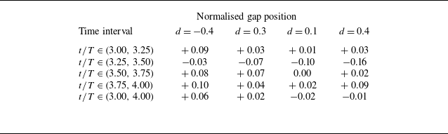
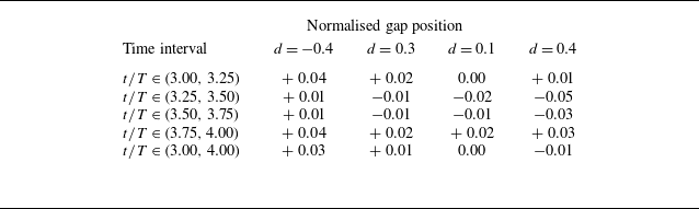
) and upstroke. Table 4 shows that the lift increments of the moult-gapped wing over the intact wing during the upstroke deceleration (
 $3.00\lt {t/T}\lt 3.25$
), downstroke deceleration (
 $3.50\lt {t/T}\lt 3.75$
) and upstroke acceleration (
 $3.75\lt {t/T}\lt 4.00$
) stages are +0.09, +0.08 and +0.10, respectively. In contrast, the downstroke acceleration stage (
 $3.25\lt {t/T}\lt 3.50$
) exhibits a decrease of 0.03. The moult-gapped wing with the normalised gap position
 $d = 0.3$
outperforms the intact wing in terms of the average nominal lift coefficient, as shown in figure 17(b). This lift enhancement is attributed to the slower decay rate during the downstroke deceleration stage (
 $3.50\lt {t/T}\lt 3.75$
), resulting in a net positive increment in lift across the downstroke deceleration (
 $3.50\lt {t/T}\lt 3.75$
), upstroke acceleration (
 $3.75\lt {t/T}\lt 4.00$
) and upstroke deceleration (
 $3.00\lt {t/T}\lt 3.25$
) stages, compensating for the loss in the downstroke acceleration stage (
 $3.25\lt {t/T}\lt 3.50$
), as detailed in table 4. The nominal drag coefficients
 ${C}_{D,n}$
for moult-gapped wings with
 $d$
of −0.4 and 0.3 are approximately that of the intact wing during downstroke (see figure 18
b). The increased drag for these configurations primarily arises during upstroke, with average drag increments of +0.04 and +0.02, respectively, relative to the intact wing (see table 5).
Increments in the average nominal lift coefficient of the moult-gapped wing compared to the intact wing at different stages.

Increments in the average nominal drag coefficient of the moult-gapped wing compared to the intact wing at different stages.

As shown in figure 19(a), the nominal lift coefficient
 ${C}_{L,n}$
of the moult-gapped wing with a moult gap near the wing mid (
 $d=0.1$
) decreases below that of the intact wing during two intervals. Specifically, a major decrease occurs in the interval
 ${3.25\lt t}/{T}\lt 3.55$
, while a minor decrease appears in the interval
 ${3.70\lt t}/{T}\lt 3.80$
. The nominal lift coefficient
 ${C}_{L,n}$
for the moult-gapped wing with a wing-tip gap (
 $d = 0.4$
) is also less than that of the intact wing during the interval
 $3.25\lt {t}/{T}\lt 3.55$
, but exceeds it during the interval
 $3.60\lt {t}/{T}\lt 3.90$
. Thus, the lift loss results from a compromise between the decrease in lift during the downstroke acceleration (
 $3.25\lt t/T\lt 3.50$
) and the possible increase in lift near downstroke reversal. Table 4 shows that the increments in the average nominal lift coefficient for both the moult-gapped wings experience a greater decrease during the downstroke acceleration stage (
 $3.25\lt t/T\lt 3.50$
) than the total increase observed in the other three stages. Moreover, the average nominal drag coefficients
 $\overline {{C}_{D,n}}$
for the moult-gapped wings with normalised gap positions
 $d$
of 0.1 and 0.4 equal that of the intact wing (see figure 19
b), which results from balanced opposite increments near the maximum flapping velocities during downstroke (at the moment
 $t/T=3.50$
) and upstroke (at the moment
 $t/T=4.00$
).
Instantaneous nominal aerodynamic force coefficients of the moult-gapped wings that lose the aerodynamic forces. (a) Nominal lift coefficient
 ${C}_{L,n}$
. (b) Nominal drag coefficient
 ${C}_{D,n}$
. The white and shaded blocks represent flapping upstroke and downstroke, respectively.

In summary, the lift of the moult-gapped wings depends on the trade-off between lift loss during downstroke acceleration (
 $3.25\lt t/T\lt 3.50$
) and lift enhancement in the subsequent three stages. Specifically, the decrease in lift near the lift peak and the increase or decrease in lift near downstroke reversal play crucial roles. Regarding the drag of the moult-gapped wings, the positive increment near the drag peak is dominant or, at the very least, balanced by the negative increment near the drag valley.
The spanwise position affects the relative velocity and interaction length between the fluid at the moult gap and the wing, regulating the generation and evolution of GVs. As the moult gap moves outwards along the span, there is an increase in the relative velocity between the fluid at the moult gap and the wing, coupled with a longer interaction length. Moult gaps located towards the outer wing generate GVs more frequently than those near the inner wing, resulting in more GVs shedding within a single stroke. This enhanced activity disrupts the attachment state of the LEVs, thereby reducing the vortex lift. The role of the local relative velocity in modulating the vortex forces through the GVs can also be revealed by the instantaneous nominal aerodynamic forces under different gap widths, as shown in figure 6. When the gap position is fixed, the changes in the local relative velocity stem from variations in the wing angular velocity caused by the elevation motion. In this scenario, the maximum local relative velocity occurs near the peak of the aerodynamic force, where the maximum lift loss is also produced.
The strengths and directions of the main vortex structures, such as the LEVs, are non-uniformly distributed along the span (Li & Nabawy Reference Li and Nabawy2024). For a typical rectangular wing, the flapping motion generates a bow-shaped LEV at the leading edge, indicating that the local direction of the LEVs changes along the span. The LEVs closely follow the straight leading edge of the wing at the wing mid. Towards the wing tip, they diverge from the leading edge owing to the influence of the TVs. At the wing root, the confined corner space forces the LEVs away from the leading edge. Overall, the vortex line representing the direction of the LEVs approximates an arcuate convex curve that bends towards the trailing edge, as depicted by the dotted line in figure 20(a). Moreover, it is equally important to recognise that the local strength of the LEVs varies along the span, peaking at the wing mid and dimnishing to its minimum value at the wing root and tip, as indicated by the size of the rotation symbol in figure 20(a). Consequently, the effect stemming from the interaction between the LEVs and GVs initially intensifies and then decreases as the moult gap moves from the wing root to the wing tip along the span. In this context, the effect of the interaction between LEVs and GVs on aerodynamic forces is most profoundly affected by the wing-mid moult gap. This is evidenced by the changes in LEVs during the downstroke acceleration stage (
 $3.25\lt t/T\lt 3.50$
), as illustrated in figure 20(b). The significant lift loss observed in the moult-gapped wing, with a normalised gap position of 0.1, is primarily attributed to this distinctive structural feature of LEVs.
Spacial structures of the LEVs of the intact wing and the moult-gapped wing with a normalised gap position of 0.1. (a) Top view. (b) Back view. The vortex structures are represented by isosurfaces of
 $Q=8$
and coloured by the normalised spanwise vorticity
 ${\omega }_{y}$
. The flow structures in the figure appear at the moment
 ${t}/{T}=3.43$
. The spanwise variations of the strength and direction of the LEVs are presented schematically in panel (a). The area enclosed by the dashed line in panel (b) shows the strong interaction between the LEVs and GVs.

The local relative velocity at the moult gap accounts for the lift loss near the lift peak. The spanwise variation in the LEVs is associated with lift enhancement or loss near downstroke reversal. The change in flapping velocity direction near downstroke reversal intensifies the coupling between velocity and vorticity in the flow, which correlates with vortex lift through the Lamb vector. The Lamb vector is known as the origin of vortical flow nonlinearity and its normalised form is written as
 \begin{equation} \boldsymbol{l}=\boldsymbol{u} \times \boldsymbol{\omega }, \end{equation}
where
 $\boldsymbol{\omega }=\boldsymbol{\nabla }\times \boldsymbol{u}$
is the dimensionless vorticity vector normalised by
 ${2{{U}_{\infty }}}/{b}$
. The spatial integral of the vertical component of the Lamb vector,
 ${{l}_{z}}={{u}_{x}}{{\omega }_{y}}-{{u}_{y}}{{\omega }_{x}}$
, measures the magnitude of the lift in unsteady vortex dynamics, and its spatial distribution can be used to reveal the contribution of the main flow structures to lift generation (Marongiu, Tognaccini & Ueno Reference Marongiu, Tognaccini and Ueno2013; Wang et al. Reference Wang, Xu, Zhang and Wang2021, Reference Wang, Liu, Xu and Wang2022).
Distribution of the vertical component of the normalised Lamb vector and its two decomposed parts. (a) Intact wing. (b) Moult-gapped wing (normalised gap position
 $d$
of −0.4). The flow structures in the figure appear at the downstroke reversal,
 ${t}/{T}=3.76$
. The spanwise distance of the slice across narrow sections of the moult-gapped wing from the symmetry plane at the wing root is 19 % of the semi-span
 $b/2$
.

Next, an analysis is conducted on the Lamb vector for the moult-gapped wing, specifically with the moult gap located close to the wing root (
 $d=-0.4$
), near downstroke reversal. Figure 21 shows the distributions of the vertical component of the Lamb vector
 $l_z$
of the moult-gapped wing, and its decomposition parts
 ${{l}_{z1}}={{u}_{x}}{{\omega }_{y}}$
and
 ${{l}_{z2}}=-{{u}_{y}}{{\omega }_{x}}$
at the moment
 ${t}/{T}=3.76$
. The inclination of the LEVs near the wing root produces spanwise and streamwise vorticities of the same order of magnitude. Both vorticity components contribute positively to the lift enhancement under the action of gap flow. For the intact wing in figure 21(a), the positive values of the vertical component
 $l_z$
of the Lamb vector in the near field are primarily concentrated in a strip region initiated at the leading edge that forms a specific angle with the upper wing surface. In contrast, the region with negative values is attached to the lower wing surface and rolls up downstream the trailing edge. Compared with the intact wing, the increment in the vertical component
 $l_z$
of the Lamb vector for the moult-gapped wing, with a moult gap proximate to the wing root, is predominantly situated in a thicker strip region. Additionally, there is an increased magnitude in the Lamb vector component
 $l_{z}$
in the region between the upper wing surface and strip region. These changes in and below the strip region stem from the decomposed parts
 $l_{z1}$
and
 $l_{z2}$
, respectively, as illustrated in figure 21(b). Further decomposition, as shown in figure 22, reveals that the thicker strip region results from the reduced recirculation zone and vertical diffusion of the spanwise vorticities of the LEVs because of gap leakage. Specifically, gap leakage not only augments the flow momentum of the separation zone above the upper wing surface, thereby reducing the recirculation velocity magnitude, but also intensifies the downwards diffusion of spanwise vorticities. Moreover, the gap leakage accumulates negative streamwise vorticities from the LEVs upstream of the leeward side, resulting in the increased magnitude of the vertical Lamb vector component in the region between the upper wing surface and strip region, as depicted in figure 22(b). The effect of the moult gap near the wing root on enhancing the lift by adjusting the LEVs is more pronounced during the upstroke acceleration stage (
 $3.75\lt t/T\lt 4.00$
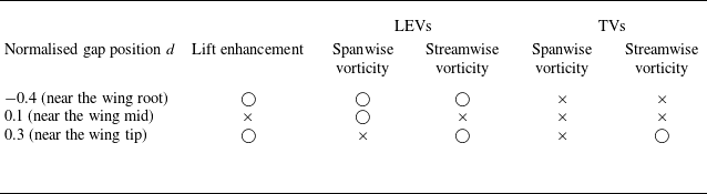
). Similar Lamb vector analyses for moult gaps near the wing tip (normalised gap position of 0.3) and near the wing mid (normalised gap position of 0.1) are provided in Appendix B. The results are summarised in table 6. The circle mark (
 $\bigcirc$
) and cross mark (
 $\times$
) represent enabled and disabled actions, respectively.
Distribution of the velocity and vorticity components at the downstroke reversal,
 ${t}/{T}=3.76$
. (a) Intact wing. (b) Moult-gapped wing (normalised gap position
 $d$
of −0.4). The spanwise distance of the slice across narrow sections of the moult-gapped wing from the symmetry plane at the wing root is 19 % of the semi-span
 $b/2$
.

Lift enhancement or loss of the moult-gapped wings with three different gap positions near downstroke reversal and identification of vorticity sources from the LEVs and TVs based on the Lamb vector analysis (
 $\bigcirc$
, enabled;
 $\times$
, disabled).

When the moult gap is at the non-wing-tip position (normalised gap position
 $d\leqslant 0.3$
), the flow topology around the moult-gapped wing differs from that of the original intact wing. By contrast, when the moult gap is at the wing tip (normalised gap position
 $d=0.4$
), the moult-gapped wing reduces to the continuous shape of the intact wing, and the flow exhibits a topology analogous to that of the intact wing. The presence of a moult gap changes the shape of the local wing tip, which directly affects the formation and evolution of the TVs. Under normal conditions, many birds form gaps in their wing tips by adjusting the vertical positions of the front primary feathers. This wing-tip configuration, similar to a winglet (Whitcomb Reference Whitcomb1976), propagates vorticity in both the horizontal and vertical directions, which can significantly reduce induced drag during gliding flight (Tucker Reference Tucker1995). The effect of the winglet-like structure on the aerodynamic performance strongly depends on its specific configuration. The experimental example under a total gap size ratio of 0 given by Lynch, Mandadzhiev & Wissa (Reference Lynch, Mandadzhiev and Wissa2018) corresponds to the moult-gapped wing with
 $d=0.4$
in this study. Their results show that the lift coefficient of gliding flight could be significantly improved owing to the wing-tip gap. Nevertheless, in flapping flight cases, the lifting-surface loss is the dominant factor. As shown in figure 19(a), the wing with a wing-tip gap loses significant lift near the lift peak but increases the lift at downstroke reversal. Because of the larger lift loss during the former stage, the average nominal lift coefficient
 $\overline {{{C}_{L,n}}}$
decreases. In contrast, the average nominal drag coefficient
 $\overline {{{C}_{D,n}}}$
remains unchanged when compared with that of the intact wing.
4. Conclusions
The role of the moult gap in a bio-inspired flapping wing model is investigated in this study. The unsteady aerodynamics and vortex dynamics of moult-gapped flapping wings are obtained by solving Navier–Stokes equations numerically. The effects of gap widths and gap positions on the aerodynamic performance and vortex structures are analysed.
The moult gap decreases the average lift and lift-to-drag ratio. However, the decrease in average lift of the moult-gapped wing is slower than that expected from the quasi-steady aerodynamic model. This is because the moult gap triggers nonlinear vortex interactions, which enhances the ability to generate lift per unit area of lifting surface (that is, the actual lift coefficient). The lift of moult-gapped wings depends on the trade-off between the reduction in the lifting surface and the enhancement in the actual lift coefficient.
The nonlinear vortex interactions alleviate the decrease in lift, which is identified as vortex compensation of the moult-gapped wing. The enhancement in the actual lift coefficient originates from the three-dimensional gap vortices attached to the gap edges. The gap vortices interact with leading-edge vortices and tip vortices, while also modifying the gap leakage flow. Consequently, the vortex system generated by each wing transforms from one vortex loop into a pair of parallelly arranged vortex loops. The vortex compensation varies as the moult gap moves along the span. On the one hand, the flapping motion increases the relative velocity and interaction length between the gap flow and wing, thereby affecting the development of gap vortices when the gap moves outwards along the span. The relative velocity accounts for the lift loss near the lift peak. On the other hand, the finite wing span causes the strength and direction of the leading-edge vortices to vary in the spanwise direction. The distribution of Lamb vector reveals that the spanwise variation in the leading-edge vortices is closely related to the lift enhancement or loss near downstroke reversal.
We model the vortex compensation as an increase in vertical induced velocity at the actuator disks reflecting the pair of parallelly arranged vortex loops. We propose a composite actuator disk model capable of predicting the average actual lift coefficient for both the intact and moult-gapped wings. This model accounts for not only the finite-span wing but also the vortex compensation effects. The proposed model captures the nonlinear interactions among the vortices around the wing in a period-averaged sense, which can be used to estimate the aerodynamic performance of a damaged flapping wing.
Funding
We gratefully acknowledge financial support from the National Natural Science Foundation of China (NSFC) Basic Science Center Program for ‘Multiscale Problems in Nonlinear Mechanics’ (Grant No. 11988102). This work is also supported by the National Natural Science Foundation of China (Grant Nos. 92252203, 12102439 and 12425207), the Chinese Academy of Sciences Project for Young Scientists in Basic Research (Grant No. YSBR-087) and the Strategic Priority Research Program of Chinese Academy of Sciences (Grant No. XDB0620102).
Declaration of interests
The authors report no conflict of interest.
Data availability statement
The data that support the findings of this work are available from the corresponding author upon reasonable request.
Appendix A. Reynolds number effects of the moult-gapped wing
An examination of Reynolds number effects is provided in this appendix. Four Reynolds numbers of the intact wing, ranging from
 $O(10^2)$
to
 $O(10^3)$
, are considered. For the moult-gapped wings at each Reynolds number, the normalised gap width
 $w$
changes from 0 to 0.3, while the normalised gap position
 $d$
is fixed at 0. The set-up of numerical simulations varies with the Reynolds number, as shown in table 7. According to our previous work (Wang et al. Reference Wang, He and Zhang2015a
; Chen, Liu & Wang Reference Chen, Liu and Wang2025), the mesh for the moult-gapped wing and its background region is refined and the time step is reduced with increasing the Reynolds number.
Set-up of numerical simulations at different Reynolds numbers.

Effect of the Reynolds number on the average nominal lift coefficient
 $\overline {{C}_{L,n}}$
. (a) Original normalised gap width
 $w$
. (b) Scaled normalised gap width
 $w/{\delta }$
.

Effect of the Reynolds number on the average actual lift coefficient
 $\overline {{C}_{L,a}}$
. (a) Original normalised gap width
 $w$
. (b) Scaled normalised gap width
 $w/{\delta }$
.

Effect of the Reynolds number on the average nominal lift-to-drag ratio
 ${\overline {{C}_{L,n}}}/{\overline {{C}_{D,n}}}$
. (a) Original normalised gap width
 $w$
. (b) Scaled normalised gap width
 $w/{\delta }$
.

Figure 23(a) plots the average nominal lift coefficient against the normalised gap width. Although the Reynolds number increases, the average nominal lift coefficient consistently exhibits a nonlinear decay, which partially mitigates the lifting-surface loss. At Reynolds numbers of 173 and 346, the moult-gapped wings with normalised gap widths
 $w \leqslant 0.1$
exhibit no decrease in the average nominal lift coefficient compared with the intact wing. When the Reynolds number increases to 693 and 1039, this non-decreasing range narrows to
 $w \leqslant 0.05$
. The range of no decrease in the average nominal lift coefficient corresponds to the range of increase in the average actual lift coefficient owing to the reduction in wing area, as displayed in figure 24(a). For the cases of
 ${\textit{Re}}=173$
and
 ${\textit{Re}}=346$
, the moult-gapped wing maintains a higher average actual lift coefficient relative to the intact wing, even at the maximum tested gap width of
 $w=0.3$
. Conversely, when
 ${\textit{Re}}=693$
and
 ${\textit{Re}}=1039$
, the moult-gapped wing with this gap width of
 $w=0.3$
shows the most reductions in the average actual lift coefficient of
 $3\,\%$
and
 $9\, \%$
, respectively, compared with the intact wing. These results suggest that the Reynolds number modulates both the magnitude and effective range of flow-induced compensation for lift loss. There is a characteristic shear layer thickness
 $\delta$
in jet flow (Goren & Wronski Reference Goren and Wronski1966). This characteristic thickness is related to the Reynolds number through
 ${\delta }=0.7{\textit{Re}}^{-1/3}$
. We use the characteristic thickness to scale the normalised gap width
 $w$
. After this scaling, the critical points of rapid decay in the average nominal lift coefficient collapse into a narrow range, as exhibited in figure 23(b). The reduced sensitivity to the Reynolds number indicates a universal mechanism associated with the vortex dynamics of the moult-gapped wing. In the narrow range of the scaled normalised gap width, the average actual lift coefficient reaches its maximum (see figure 24
b).
In figure 25, the average nominal (or actual) lift-to-drag ratio increases with the Reynolds number at a normalised gap width. Across varying Reynolds numbers, the average nominal lift-to-drag ratio generally decreases with increasing the normalised gap width, while exhibiting one or more local maxima whose positions shift with the Reynolds number. This implies that the Reynolds number affects the competition between the reduction in the lifting-surface area and the increase in the lift/drag per unit area under small gap widths.
The Reynolds number makes these effects through changing the vortex structures and their interactions. While the evolution of LEVs and TVs is modulated by the Reynolds number, the GVs maintain their essential characteristics without qualitative changes, as exhibited in figure 26. The streamwise vorticity of the GVs retains robust distribution, likely due to the aft positioning of the moult gap. The characteristic size of the vortex structures decreases as the Reynolds number increases, as shown in figure 27. There is no distinct vortex breakdown even for the maximum tested Reynolds number.
Although the Reynolds number exerts limited effects on the basic characteristics of large-scale vortex structures and their contribution to lift generation (Liu et al. Reference Liu, Wang and Liu2024), the extended Reynolds number ranges are essential for quantifying the real flight of birds or micro-air vehicles, which is accounted for in further work.
Effect of Reynolds number on gap vortices (GVs). The plot shows the distribution of the normalised streamwise vorticity
 ${\omega }_{x}$
around the moult-gapped wing with a normalised gap width
 $w$
of 0.2. The slices are extracted at the normalised streamwise position
 $2x/b=0.1$
around the moment
 ${t}/{T}=3.30$
.

Effect of Reynolds number on global vortices. The plot exhibits the top view of the moult-gapped wing with a normalised gap width
 $w$
of 0.2 around the moment
 ${t}/{T}=3.30$
. The vortex structures are represented by isosurfaces of
 $Q=3$
and coloured by the normalised spanwise vorticity
 ${\omega }_{y}$
.

Appendix B. Lamb vector field of the moult-gapped wings with the moult gaps at two typical positions
Distribution of the vertical component of the normalised Lamb vector and its two decomposed parts. (a) Intact wing. (b) Moult-gapped wing (normalised gap position
 $d$
of 0.3). The flow structures in the figure appear at the downstroke reversal,
 ${t}/{T}=3.76$
. The spanwise distance of the slice across narrow sections of the moult-gapped wing from the symmetry plane at the wing root is 84 % of the semi-span
 $b/2$
. This view is from the wing tip to the wing root.

Distribution of the velocity and vorticity components at the downstroke reversal,
 ${t}/{T}=3.76$
. (a) Intact wing. (b) Moult-gapped wing (normalised gap position
 $d$
of 0.3). The spanwise distance of the slice across narrow sections of the moult-gapped wing from the symmetry plane at the wing root is 84 % of the semi-span
 $b/2$
. This view is from the wing tip to the wing root.

This appendix first shows the distribution characteristics of the Lamb vector around the moult-gapped wing with a moult gap near the wing tip (normalised gap position
 $d$
of 0.3). The degree of inclination of the LEVs near the wing tip is higher because of the interference of the TVs. The streamwise vorticities of the LEVs and TVs contribute to the lift enhancement of the moult-gapped wing. As shown in figure 28(a), the near-wing-tip section of the intact wing exhibits an additional strip region with a positive Lamb vector component
 $l_{z}$
compared with the near-wing-root section in figure 21. This region results from the decomposed part
 $l_{z2}$
of the vertical Lamb vector component
 $l_z$
. The increase in the Lamb vector component
 $l_z$
within the same section of the moult-gapped wing with a normalised gap position
 $d$
of 0.3 is attributed to the thickening of the new strip region and an increased positive Lamb vector component
 $l_z$
between the upper wing surface and the upstream original strip region, as illustrated in figure 28(b). In comparison, both increases arise from the decomposed part
 ${l}_{z2}$
. As observed in figure 29, the gap leakage expands the region of positive spanwise velocity that points towards the wing tip, allowing the negative streamwise vorticity of the TVs to obtain a more positive spanwise velocity. Consequently, this process consequently thickens the new strip region. Furthermore, the increase in the positive Lamb vector component
 $l_z$
between the upper wing surface and the original strip region is also attributed to the accumulation of positive streamwise vorticities from the LEVs upstream of the gap flow.
The following presents the distribution characteristics of the Lamb vector around the moult-gapped wing with a moult gap near the wing mid (normalised gap position
 $d$
of 0.1). The LEVs have the largest strength near the wing mid, with the direction almost parallel to the leading edge of the moult-gapped wing. The lift loss caused by the strong interference between the gap flow and LEVs is primarily associated with the spanwise vorticities of the LEVs. As shown in figure 30, the change in the vertical component
 ${l}_{z}$
of the Lamb vector for the moult-gapped wing compared with the intact wing is characterised by an enlargement of the region with a negative vertical component
 ${l}_{z}$
above the trailing edge. This change is dominated by the decomposed part
 ${l}_{z1}$
of the vertical component of the Lamb vector. Under the strong interaction between the LEVs and GVs, the recirculation zone beneath the LEVs expands unexpectedly, as observed in figure 31. Moreover, some spanwise vorticities of the LEVs enter the expanded recirculation zone, thereby causing a small portion of the lift to be lost near downstroke reversal.
Distribution of the vertical component of the normalised Lamb vector and its two decomposed parts. (a) Intact wing. (b) Moult-gapped wing (normalised gap position
 $d$
of 0.1). The flow structures in the figure appear at the downstroke reversal,
 ${t}/{T}=3.76$
. The spanwise distance of the slice across narrow sections of the moult-gapped wing from the symmetry plane at the wing root is 61 % of the semi-span
 $b/2$
.

Distribution of the velocity and vorticity components at the downstroke reversal,
 ${t}/{T}=3.76$
. (a) Intact wing. (b) Moult-gapped wing (normalised gap position
 $d$
of 0.1). The spanwise distance of the slice across narrow sections of the moult-gapped wing from the symmetry plane at the wing root is 61 % of the semi-span
 $b/2$
.

Appendix C. Limitations and potential applications
As a first step to investigate the moult-gapped flapping wing, we focus on the aerodynamic effects and vortex dynamics associated with different gap widths and gap positions. The numerical simulation is employed owing to its high spatio-temporal resolution of the near-wall vorticity. However, multiple physical factors that affect the aerodynamic performance of moult-gapped wings are not considered in this study, including the wing flexibility and aspect ratio. These additional physical factors can be addressed by combined numerical and experimental approaches. The experiments provide a crucial complement when actual flapping wings are included. Here, we take the wing flexibility as an example to discuss the possible effects of the additional physical factors. The potential applications of the current study are also provided.
The flexibility of flapping wings is generally distributed along the chordwise or spanwise direction (Shyy et al. Reference Shyy, Aono, Chimakurthi, Trizila, Kang, Cesnik and Liu2010). For the two-dimensional hovering wing, appropriate chordwise flexibility can improve aerodynamic performance by modulating the evolution of leading-edge vortices and their interaction with trailing-edge vortices (Eldredge, Toomey & Medina Reference Eldredge, Toomey and Medina2010). In forward flight, the flapping wing with the spanwise flexibility reaches its optimal aerodynamic performance when the prescribed flapping frequency approximates to the first natural frequency of the structure (Martínez-Muriel et al. Reference Martínez-Muriel, Arranz, García-Villalba and Flores2023). Under this condition, the effective angles of attack of the outboard wing sections become larger and the development of the leading edge vortices is delayed. Nevertheless, excessive chordwise and spanwise flexibility may conversely degrade the aerodynamic performance. While the wing flexibility modulates the aerodynamic characteristics, its coupling with large-scale vortices exhibits universal behaviour. Zhang et al. (Reference Zhang, Huang and Lu2020) numerically investigate the propulsive performance of heaving flexible plates with different trailing-edge shapes. The degree of flexibility is measured by the bending stiffness
 $K$
. The plate with the concave trailing edge has certain similar characteristics to the moult-gapped wing model in our study. For plates with large bending stiffness (
 $K \in [22,25]$
), the concave trailing-edge plate exhibits superior performance compared with the straight trailing-edge plate. Conversely, at low-to-moderate bending stiffness levels (
 $K \in [2,10]$
), the concave trailing-edge plate underperforms the straight trailing-edge counterpart. In addition, at the large bending stiffness, the strength of leading-edge vortices decreases when the trailing edge changes from the straight profile to the concave one. Moreover, the concave trailing-edge plate causes reversed horseshoe vortices, corresponding to the gap vortices of the moult-gapped wings. The horseshoe vortices are not significantly affected by the bending stiffness.
The potential applications of this work in the damage-coping response and fault-tolerant design of micro-air vehicles (Salem et al. Reference Salem, Cellini, Kabutz, Hari Prasad, Cheng, Jayaram and Mongeau2022) are as follows. Similar to the flying animals, micro-air vehicles experience degradation in critical flight performance when sustaining wing damage, given the inherent instability of flapping flight. The change in the average/instantaneous aerodynamic force coefficients caused by the wing gap could be used to develop an onboard fault-tolerant flight controller (Shekar, LeBeau & Gururajan Reference Shekar, LeBeau and Gururajan2022), which can monitor abrupt variations in the flight dynamics and activate compensatory kinematics to stabilise the micro-air vehicles. With this ability, the micro-air vehicles decide either to continue its predefined task or execute safe and controlled landing. Towards the goal, the numerical or experimental data, such as the results of our work, can be taken as input of machine learning algorithm to detect and classify the wing damage (Shekar et al. Reference Shekar, LeBeau and Gururajan2022, Reference Shekar, LeBeau and Gururajan2023). A prototype of this fault-tolerant flight controller has been implemented by mimicking the damage-coping response of flies (Salem et al. Reference Salem, Cellini, Kabutz, Hari Prasad, Cheng, Jayaram and Mongeau2022). Both active (adaptive) and passive (robust) controls are applied to handle various wing damages.