1 Introduction
Double-diffusive convection in porous media, driven by both temperature and concentration gradients, has been the subject of intensive research in view of its importance in many natural and industrial problems. Such applications include ground water pollution, geothermal systems, crude oil production, storage of energy, underground diffusion of nuclear wastes, solidification of binary mixtures, and so on. An overview of the current state of the art on this topic was conducted recently by Ingham & Pop (Reference Ingham and Pop1998, Reference Ingham and Pop2005), Vafai (Reference Vafai2005), Vadasz (Reference Vadasz2008) and Nield & Bejan (Reference Nield and Bejan2013).
Nield (Reference Nield1968) and Taunton, Lightfoot & Green (Reference Taunton, Lightfoot and Green1972) were first to study double-diffusive convection in a porous layer modelled according to Darcy’s law, which is relevant to densely packed and low-permeability porous media. Relying on linear stability theory on an initially motionless stable concentration stratified horizontal porous layer heated and salted from the bottom, the onset of motion was predicted. More recently, the Soret and Dufour effects on the onset of convection in a porous layer were investigated by Motsa (Reference Motsa2008). The onset of double-diffusive convection in a porous cavity subject to mixed boundary conditions was studied numerically by Mahidjiba, Mamou & Vasseur (Reference Mahidjiba, Mamou and Vasseur2000). Both Mahidjiba et al. (Reference Mahidjiba, Mamou and Vasseur2000) and Motsa (Reference Motsa2008) predicted the critical Rayleigh number for the onset of motion in terms of the governing parameters of the problem and in particular the aspect ratio of the enclosure and the various boundary conditions imposed on the system.
Finite-amplitude convection, in a two-component fluid-saturated porous layer, has been considerably investigated in the past. For instance, on the basis of Fourier series, Nield, Manole & Lage (Reference Nield, Manole and Lage1993), using a low-order Galerkin approximation, investigated theoretically convection induced by inclined thermal and solutal gradients in a horizontal porous layer. The onset and development of double-diffusive convection in a rectangular cavity subject to vertical gradients of heat and solute were investigated analytically and numerically by Mamou & Vasseur (Reference Mamou and Vasseur1999). It was demonstrated by these authors, on the basis of the parallel flow approximation, that the onset of motion from the rest state was subcritical when the buoyancy forces were opposing each other and the Lewis number was greater than unity. Moreover, the existence of multiple solutions, for a given set of the governing parameters, and the possible occurrence of travelling waves in a shallow enclosure were demonstrated numerically. Double-diffusive and Soret-induced convection in a shallow horizontal porous layer subject to Neumann boundary conditions was investigated by Bahloul, Boutana & Vasseur (Reference Bahloul, Boutana and Vasseur2003). An asymptotic analytical solution of the steady form of the governing equations, valid in the limit of an infinite layer, was derived by these authors. The critical Rayleigh numbers for the onset of supercritical and subcritical convection, as well as expressions for the Nusselt and Sherwood numbers, were obtained explicitly in terms of the governing parameters. The same problem was reconsidered by Alloui, Bennacer & Vasseur (Reference Alloui, Bennacer and Vasseur2009), taking into account the variation of permeability within the porous layer. The problem of thermosolutal convection in a shallow cavity subject to cross-fluxes of heat and mass was investigated by Kalla et al. (Reference Kalla, Mamou, Vasseur and Robillard2001). It was found that, for subcritical convection conditions, up to five different solutions were possible for a given set of governing parameters. The analytical predictions were validated with numerical simulations of the full governing equations. Soret-driven convection in a shallow cavity exposed to uniform heat fluxes was considered by Bahloul, Vasseur & Robillard (Reference Bahloul, Vasseur and Robillard2007). The imperfection caused by a horizontal temperature gradient to the standard Bénard bifurcations (supercritical or subcritical) was discussed. Moreover, the existence of transcritical bifurcations was demonstrated. Natural convection in a porous layer heated and salted from below and subject to a horizontal heat flux was investigated by Mansour et al. (Reference Mansour, Amahmid, Hasnaoui and Mamou2007). The particular case for which an equilibrium state existed between the horizontal heat flux and the induced Soret mass flux, for which a rest state solution was possible, was considered by these authors. It was found, analytically and numerically, that five distinct regions describing different flow behaviours were possible. The stability of the rest state and convective states within a shallow porous layer, modelled according to Hazen–Darcy law, was studied by Mamou (Reference Mamou2003). Considering various combinations of Dirichlet and Neumann thermal and solution boundary conditions, the thresholds for the onset of overstability and Hopf bifurcation were predicted as a function of the governing parameters. Both thresholds were found to depend considerably on the acceleration coefficient and the normalized porosity of the porous medium.
All of the above studies relied on Darcy’s law, which is relevant to densely packed low-porosity and permeability porous media. This model is valid only when the pore-diameter-related Reynolds number is less than unity. However, when the permeability of the porous medium is high enough, the drag effect due to the solid matrix and the viscous stresses near the solid walls may become non-negligible. To take into account these non-Darcy effects, both the Dupuit (Reference Dupuit1863) (or Forchheimer Reference Forchheimer1901) and the Brinkman (Reference Brinkman1949) terms must be included in Darcy’s law. Nield & Bejan (Reference Nield and Bejan2013) provided a comprehensive review literature survey of non-Darcy natural convection in porous media. The majority of the research effort was devoted to flows caused by a single buoyancy effect (thermal convection). A few studies were also reported on non-Darcy effects on double-diffusive convection, in a cavity filled with a porous medium saturated by a binary fluid. Karimi-Fard, Charrier-Mojtabi & Vafai (Reference Karimi-Fard, Charrier-Mojtabi and Vafai1997) used the Brinkman–Forchheimer-extended Darcy equation to study the influence of the form drag and boundary effects on double-diffusive convection in a vertical porous layer. It was observed that the heat and mass transfer increased with increase in Darcy number and decrease of the form drag parameter. Moreover, it was found that, for a given value of the form drag parameter, the heat transfer was maximized for a critical value of the Schmidt number. Shivakumara & Sumithra (Reference Shivakumara and Sumithra1999), using both linear and nonlinear stability theories, relied on the Brinkman-extended Darcy flow model to study the non-Darcian effects on double-diffusive convection in a horizontal sparsely packed porous layer. Depending on the values of the physical parameters, it was demonstrated that the onset of motion might be either supercritical or subcritical. It was observed that Hopf bifurcation always occurs at a lower value of the Rayleigh number than the one obtained for simple bifurcation. Moreover, the condition for the transition from oscillatory to direct instability was derived. The effect of temperature modulation on the onset of double-diffusive convection in a porous layer, modelled according to the Brinkman–Forchheimer-extended Darcy equation, was studied by Bhadauria (Reference Bhadauria2007). On the basis of linear stability theory it was demonstrated that the effect of decreasing Darcy number is to decrease the value of the critical Rayleigh number. The results corresponding to the Brinkman model and the Darcy model were compared and correlated. The Soret effect in a horizontal sparsely packed porous layer was investigated by Gaikwad & Kamble (Reference Gaikwad and Kamble2012). The Rayleigh numbers for both stationary and oscillatory convection were derived using linear stability analysis. Khanafer & Vafai (Reference Khanafer and Vafai2002) conducted a numerical analysis of double-diffusive mixed convection in a lid-driven enclosure filled with a fluid-saturated porous medium, considering non-Darcian effects.
Recently, the effect of form drag on natural thermal convection in a shallow porous layer heated from below was studied by Rebhi, Mamou & Alliche (Reference Rebhi, Mamou and Alliche2014), considering the Dupuit-extended Darcy model. The form drag was found to have a significant impact on the convective heat transfer. Moreover, although the form drag effect had no influence on the thresholds for the onset of stationary motion, it was demonstrated to have a strong effect on the onset of Hopf bifurcation. As the form drag has a stabilizing effect on the convective flow, it is believed to have a considerable effect on the onset of subcritical convection in opposing double-diffusive convection. This point is the subject of the present study. Neumann/Dirichlet thermal and solutal boundary conditions are applied on the horizontal walls of the cavity. The case of opposing thermal and concentration buoyancy forces is considered. For this situation, it is well known that, for a given set of governing parameters, the onset of motion may be subcritical, i.e. occur at finite amplitude convection well below the thresholds of stationary convection (see, for instance, Mamou & Vasseur Reference Mamou and Vasseur1999). More recently, Rebhi et al. (Reference Rebhi, Mamou, Vasseur and Alliche2016) investigated the form drag effect on Soret convection within a tall porous cavity. It was reported that, for the situation where the buoyancy forces are equal and opposing each other, the onset of subcritical convection was significantly affected by the form drag, which played a role as a stabilizing effect. Multiple steady-state and oscillatory solutions coexisted near criticality, and vertically travelling waves were observed. To the best of the authors’ knowledge, the effect of the form drag parameter on subcritical bifurcation in Lapwood convection does not seem to have been investigated systematically in the past. A new bistability phenomenon is demonstrated in the present study, for which two steady-state solutions with similar flow patterns coexist near the onset of stationary convection.
This paper is organized as follows. In § 2, the governing equations describing the problem are derived. Section 3 describes the numerical method used to solve the problem. An approximate analytical solution, obtained on the basis of a steady parallel flow approximation, is proposed in § 4. A linear stability analysis is presented in § 5 in order to predict the onset of Hopf bifurcation; transition from stationary to oscillatory convection. The results are discussed in § 6 and a conclusion is presented in § 7.
2 Mathematical formulation
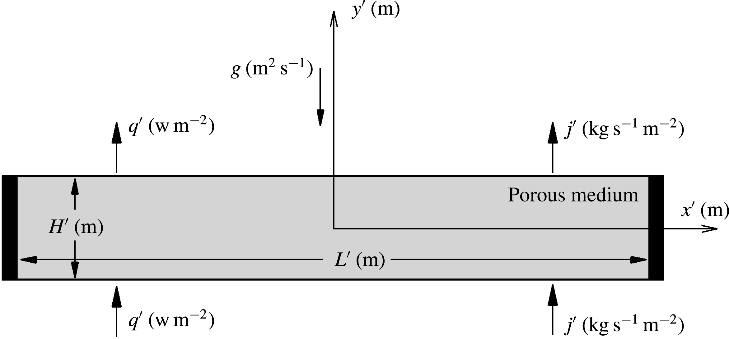
The configuration considered in this study is a horizontal shallow porous cavity, of thickness
 $H^{\prime }$
and length
 $L^{\prime }$
, filled with a binary mixture (see figure 1). The origin of the coordinate system is located at the centre of the cavity, with
 $x^{\prime }$
and
 $y^{\prime }$
being the horizontal and vertical coordinates respectively. All of the boundaries are impermeable. Neumann boundary conditions are applied, for both temperature and concentration, on the horizontal walls of the layer. The binary fluid is assumed to satisfy the Boussinesq approximation. The density variation with temperature and concentration is described by the state equation as
 $\unicode[STIX]{x1D70C}=\unicode[STIX]{x1D70C}_{0}[1-\unicode[STIX]{x1D6FD}_{T}^{\prime }(T^{\prime }-T_{0}^{\prime })-\unicode[STIX]{x1D6FD}_{N}(N-N_{0})]$
, where
 $\unicode[STIX]{x1D70C}_{0}$
is the fluid mixture density at temperature
 $T^{\prime }=T_{0}^{\prime }$
and mass fraction
 $N=N_{0}$
, and
 $\unicode[STIX]{x1D6FD}_{T}^{\prime }$
and
 $\unicode[STIX]{x1D6FD}_{N}$
are the thermal and concentration expansion coefficients respectively. The equations relating the fluxes of heat,
 $q^{\prime }$
, and matter,
 $j^{\prime }$
, to the thermal and solute gradients present in the binary fluid mixture are given by
 $q^{\prime }=-k\unicode[STIX]{x1D735}T^{\prime }$
and
 $j^{\prime }=-\unicode[STIX]{x1D70C}D\unicode[STIX]{x1D735}N$
, where
 $k$
and
 $D$
are the thermal conductivity and the isothermal diffusion coefficient respectively.
Schematic diagram of the problem domain and coordinate system.

The governing equations that describe the convective behaviour of the system are conservation of mass, momentum, energy and species, stated as follows using the conservative form assuming incompressible flow (see, for instance, Rebhi et al. Reference Rebhi, Mamou and Alliche2014, Reference Rebhi, Mamou, Vasseur and Alliche2016):
 $$\begin{eqnarray}\displaystyle & \displaystyle \frac{\unicode[STIX]{x2202}u}{\unicode[STIX]{x2202}x}+\frac{\unicode[STIX]{x2202}v}{\unicode[STIX]{x2202}y}=0, & \displaystyle\end{eqnarray}$$
 $$\begin{eqnarray}\displaystyle & \displaystyle -\frac{\unicode[STIX]{x2202}P}{\unicode[STIX]{x2202}x}=\left(1+\frac{V_{a}}{P_{r}^{\ast }}\right)u, & \displaystyle\end{eqnarray}$$
 $$\begin{eqnarray}\displaystyle & \displaystyle -\frac{\unicode[STIX]{x2202}P}{\unicode[STIX]{x2202}y}=\left(1+\frac{V_{a}}{P_{r}^{\ast }}\right)v-R_{T}(T+\unicode[STIX]{x1D711}S), & \displaystyle\end{eqnarray}$$
 $$\begin{eqnarray}\displaystyle & \displaystyle \frac{\unicode[STIX]{x2202}T}{\unicode[STIX]{x2202}t}+\frac{\unicode[STIX]{x2202}(uT)}{\unicode[STIX]{x2202}x}+\frac{\unicode[STIX]{x2202}(vT)}{\unicode[STIX]{x2202}y}=\unicode[STIX]{x1D6FB}^{2}T, & \displaystyle\end{eqnarray}$$
 $$\begin{eqnarray}\displaystyle & \displaystyle \unicode[STIX]{x1D700}\frac{\unicode[STIX]{x2202}S}{\unicode[STIX]{x2202}t}+\frac{\unicode[STIX]{x2202}(uS)}{\unicode[STIX]{x2202}x}+\frac{\unicode[STIX]{x2202}(vS)}{\unicode[STIX]{x2202}y}=Le^{-1}\unicode[STIX]{x1D6FB}^{2}S, & \displaystyle\end{eqnarray}$$
where the variables
 $u$
and
 $v$
are respectively the dimensionless horizontal and vertical dimensionless velocity components,
 $V_{a}=\sqrt{u^{2}+v^{2}}$
is the dimensionless velocity magnitude,
 $P$
is the dimensionless pressure,
 $T$
is the dimensionless temperature,
 $S$
is the dimensionless concentration,
 $t$
is the dimensionless time and
 $\unicode[STIX]{x1D700}$
is the normalized porosity of the porous medium.
The dimensionless boundary conditions applied on the walls of the cavity are
 $$\begin{eqnarray}u=0,\quad \frac{\unicode[STIX]{x2202}T}{\unicode[STIX]{x2202}x}=\frac{\unicode[STIX]{x2202}S}{\unicode[STIX]{x2202}x}=0,\quad \text{at}~x=\pm \frac{A}{2},\end{eqnarray}$$
 $$\begin{eqnarray}v=0,\quad \frac{\unicode[STIX]{x2202}T}{\unicode[STIX]{x2202}y}=\frac{\unicode[STIX]{x2202}S}{\unicode[STIX]{x2202}y}=-1,\quad \text{at}~y=\pm \frac{1}{2}.\end{eqnarray}$$
The above equations were non-dimensionalized by introducing the following scales (primed quantities are dimensional):
 $$\begin{eqnarray}\left.\begin{array}{@{}c@{}}(x,y)=(x^{\prime },y^{\prime })/H^{\prime },\quad (u,v)=(u^{\prime },v^{\prime })H^{\prime }/\unicode[STIX]{x1D6FC},\\ t=t^{\prime }\unicode[STIX]{x1D6FC}/H^{\prime 2},\quad \unicode[STIX]{x1D700}=\unicode[STIX]{x1D719}/\unicode[STIX]{x1D70E},\\ T=(T^{\prime }-T_{0}^{\prime })/\unicode[STIX]{x0394}T^{\prime },\quad S=N/\unicode[STIX]{x0394}N,\\ P=P^{\prime }K/\unicode[STIX]{x1D708}\unicode[STIX]{x1D70C}\unicode[STIX]{x1D6FC},\end{array}\right\}\end{eqnarray}$$
where
 $\unicode[STIX]{x0394}T^{\prime }=q^{\prime }H^{\prime }/k$
and
 $\unicode[STIX]{x0394}N=j^{\prime }/\unicode[STIX]{x1D70C}D$
,
 $\unicode[STIX]{x1D6FC}$
is the thermal diffusivity of the porous medium and
 $\unicode[STIX]{x1D70E}=(\unicode[STIX]{x1D70C}C)_{P}/(\unicode[STIX]{x1D70C}C)_{f}$
is the heat capacity ratio;
 $(\unicode[STIX]{x1D70C}C)_{f}$
and
 $(\unicode[STIX]{x1D70C}C)_{p}$
are the heat capacities of the fluid and the saturated porous medium respectively.
From the above equations, it is observed that the present problem is controlled by six governing parameters, namely the Rayleigh number,
 $R_{T}$
, the modified Prandtl number,
 $P_{r}^{\ast }$
, the Lewis number,
 $Le$
, the buoyancy ratio,
 $\unicode[STIX]{x1D711}$
, the normalized porosity,
 $\unicode[STIX]{x1D700}$
, and the aspect ratio of the enclosure,
 $A$
:
 $$\begin{eqnarray}\left.\begin{array}{@{}c@{}}\displaystyle R_{T}=\frac{g\unicode[STIX]{x1D6FD}_{T}^{\prime }\unicode[STIX]{x0394}T^{\prime }KH^{\prime }}{\unicode[STIX]{x1D6FC}\unicode[STIX]{x1D708}},\quad P_{r}^{\ast }=\frac{\unicode[STIX]{x1D708}H^{\prime }}{\unicode[STIX]{x1D6FC}C_{DF}K^{1/2}},\quad Le=\frac{\unicode[STIX]{x1D6FC}}{D},\\ \displaystyle \unicode[STIX]{x1D711}=\frac{\unicode[STIX]{x1D6FD}_{N}\unicode[STIX]{x0394}N}{\unicode[STIX]{x1D6FD}_{T}^{\prime }\unicode[STIX]{x0394}T^{\prime }},\quad \unicode[STIX]{x1D700}=\frac{\unicode[STIX]{x1D719}}{\unicode[STIX]{x1D70E}},\quad A=\frac{L^{\prime }}{H^{\prime }},\end{array}\right\}\end{eqnarray}$$
where
 $g$
is the gravitational acceleration,
 $\unicode[STIX]{x1D708}$
is the kinematic viscosity of the fluid,
 $K$
is the porous matrix permeability and
 $C_{DF}$
is a coefficient related to a form or pressure drag.
The overall form drag coefficient defined in terms of the modified Prandtl number is a combination of two dimensionless parameters (
 $P_{r}^{\ast }=P_{r}/F_{s}$
), the Prandtl number,
 $P_{r}$
, and the Forchheimer number,
 $F_{s}=C_{DF}Da^{1/2}$
. According to Beavers, Sparrow & Rodenz (Reference Beavers, Sparrow and Rodenz1973) and Nield & Bejan (Reference Nield and Bejan2013), the adapted form drag coefficient, within a bounded porous shallow layer, filled with beads, can be estimated from the following relationship:
 $C_{DF}=0.55[1-2.75(1+1/A)d^{\prime }/H^{\prime }]$
, where
 $d^{\prime }$
is the bead diameter. As an example of practical small or big values of
 $P_{r}^{\ast }$
, if we consider an infinite porous layer,
 $A\gg 1$
, with a characterized Darcy number of order
 ${\sim}10^{-4}$
or larger, and assume
 $d^{\prime }/H^{\prime }\ll 1$
, it can be easily seen that the modified Prandtl number can be close to unity (
 $P_{r}^{\ast }\sim 1$
) for metal liquids (
 $P_{r}\sim 10^{-3}$
) or very large (
 $P_{r}^{\ast }\gg 1$
) for gas (i.e. air) and other liquids (i.e. water, oils and polymers).
In the literature, it appears that there is still some confusion around the physical meaning of the quadratic term in the motion equation, which is attributed to the Forchheimer or Dupuit effect. Some of the previous studies stated that the quadratic term represents the inertial drag, while for some others it quantifies the form or pressure drag; see, for instance, just to give a few references, Lage (Reference Lage, Ingham and Pop1998), Vafai (Reference Vafai2005) and Lasseux, Abbasian Arani & Ahmadi-Senichault (Reference Lasseux, Abbasian Arani and Ahmadi-Senichault2011). Therefore, it is worth reiterating that, according to the literature (Joseph, Nield & Papanicolaou Reference Joseph, Nield and Papanicolaou1982; Lage Reference Lage, Ingham and Pop1998; Nield Reference Nield2000; Nield & Bejan Reference Nield and Bejan2013; Rebhi et al. Reference Rebhi, Mamou and Alliche2014), the quadratic term in the Dupuit–Darcy equation is in fact linked to a form or pressure drag with irrefutable physical explanation.
In the present study, two dimensionless parameters,
 $P_{r}^{\ast }$
and
 $\unicode[STIX]{x1D700}$
, are introduced to reduce the number of governing parameters. The parameter
 $P_{r}^{\ast }$
combines the effects of the Prandtl and Forchheimer numbers and
 $\unicode[STIX]{x1D700}$
the effects of the porous matrix porosity
 $\unicode[STIX]{x1D711}$
and the heat capacity ratio
 $\unicode[STIX]{x1D70E}$
. Most of the governing parameter value ranges are chosen from the literature to illustrate the effect of the form drag on the flow behaviour and heat and mass transfer rates.
In order to satisfy the continuity equation, a stream function
 $\unicode[STIX]{x1D6F9}$
is defined such that
 $u=\unicode[STIX]{x2202}\unicode[STIX]{x1D6F9}/\unicode[STIX]{x2202}y$
and
 $v=-\unicode[STIX]{x2202}\unicode[STIX]{x1D6F9}/\unicode[STIX]{x2202}x$
. Eliminating the pressure from (2.2) and (2.3) in the usual way, the momentum equation in terms of the stream function is given by
 $$\begin{eqnarray}\left(1+\frac{V_{a}}{P_{r}^{\ast }}\right)\unicode[STIX]{x1D6FB}^{2}\unicode[STIX]{x1D6F9}+\frac{1}{P_{r}^{\ast }V_{a}}\left(v^{2}\frac{\unicode[STIX]{x2202}^{2}\unicode[STIX]{x1D6F9}}{\unicode[STIX]{x2202}x^{2}}+u^{2}\frac{\unicode[STIX]{x2202}^{2}\unicode[STIX]{x1D6F9}}{\unicode[STIX]{x2202}y^{2}}-2uv\frac{\unicode[STIX]{x2202}^{2}\unicode[STIX]{x1D6F9}}{\unicode[STIX]{x2202}x\unicode[STIX]{x2202}y}\right)=-R_{T}\frac{\unicode[STIX]{x2202}}{\unicode[STIX]{x2202}x}(T+\unicode[STIX]{x1D711}S).\end{eqnarray}$$
The heat and mass transfer rates, expressed in terms of the Nusselt and Sherwood numbers, can be computed from the following expressions:
 $$\begin{eqnarray}Nu=\frac{1}{\unicode[STIX]{x0394}T},\quad Sh=\frac{1}{\unicode[STIX]{x0394}S},\end{eqnarray}$$
where
 $\unicode[STIX]{x0394}T=T(x,-1/2)-T(x,1/2)$
and
 $\unicode[STIX]{x0394}S=S(x,-1/2)-S(x,1/2)$
are the temperature and concentration differences, evaluated at any
 $x$
position.
For a finite aspect ratio enclosure, it is of interest to quantify the heat transfer and mass transfer rates in terms of the average Nusselt and Sherwood numbers,
 $Nu_{m}$
and
 $Sh_{m}$
, defined respectively as
 $$\begin{eqnarray}\left.\begin{array}{@{}l@{}}\displaystyle Nu_{m}=\frac{1}{A}\int _{-A/2}^{+A/2}Nu\,\text{d}x,\\ \displaystyle Sh_{m}=\frac{1}{A}\int _{-A/2}^{+A/2}Sh\,\text{d}x.\end{array}\right\}\end{eqnarray}$$
3 Numerical solution
The governing equations (2.4), (2.5) and (2.9) with the specified boundary conditions in (2.6) were solved numerically using a finite difference method. Central differencing was used to approximate the advection–diffusion terms, i.e. the scheme is second-order accurate in space. The governing equations were converted into a system of algebraic equations through their discretization at each internal grid node. The algebraic equations were solved by a line-by-line iterative method. The method sweeps the domain of integration along the
 $x$
- and
 $y$
-axes and uses tridiagonal matrix inversion to solve the resulting system of equations. The stream function equation (2.9) was solved by the SOR (successive over-relaxation) method. Starting from given specified initial values of variables, the dimensionless time step that yielded convergence for the majority of cases was up to
 $\unicode[STIX]{x0394}t=10^{-3}$
. At each new time step, updating of the physical new variable,
 $\unicode[STIX]{x1D6F9}$
, was done until the convergence criterion
 $\sum _{i,j=1}^{m}(\unicode[STIX]{x1D6F9}_{i,j}^{k}-\unicode[STIX]{x1D6F9}_{i,j}^{k-1})/\sum _{i,j=1}^{m}\unicode[STIX]{x1D6F9}_{i,j}^{k}\leqslant 10^{-6}$
was satisfied. The subscripts
 $i$
and
 $j$
denote grid locations in the
 $(x,y)$
plane,
 $m$
is the node number in either
 $x$
- or
 $y$
-direction, and
 $k$
represents the
 $k$
th iteration within the SOR iterative procedure. A further decrease of the convergence criterion did not cause any significant change in the final results. Convergence with mesh size was verified by employing coarser and finer grids on selected test problems. Based on these results, a mesh size of
 $400\times 200$
was adopted for most of the cases considered in this study. Most of the numerical results presented here were obtained for a cavity with an aspect ratio of
 $A=10$
. However, a few results were included to demonstrate the aspect ratio effect on the existence of the bistability phenomenon.
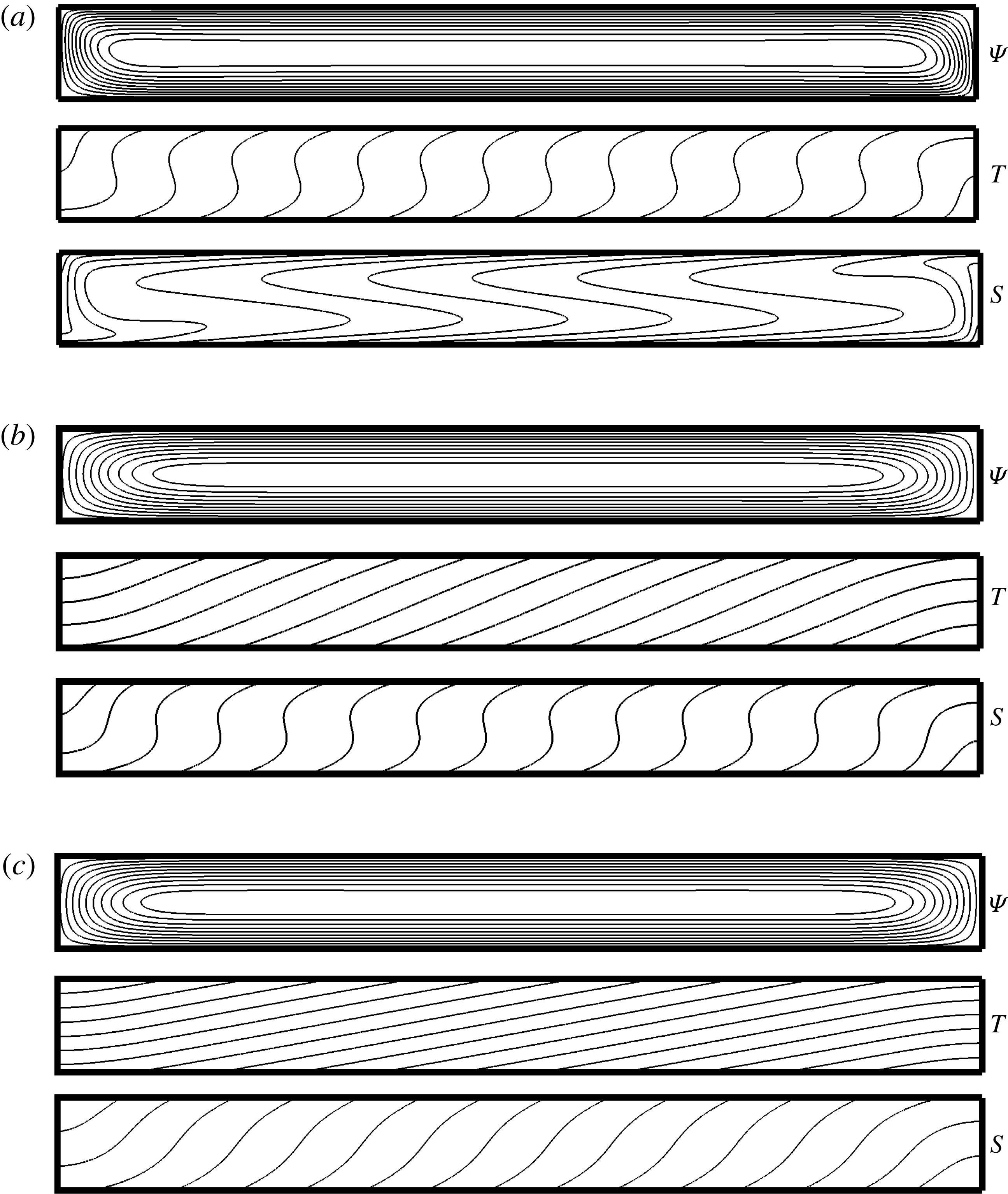
Typical numerical results are presented in figure 2(a–c) for various values of the governing parameters. In these graphs, streamlines, isotherms and isoconcentrates are presented from top to bottom. The results clearly illustrate the fact that for a shallow cavity,
 $(A\gg 1)$
, the flow in the core region of the enclosure is essentially parallel, while the temperature and concentration in the core are linearly stratified in the horizontal directions. The analytical solution, developed in the following section, relies on these physical observations.
4 Nonlinear analytical solution
In the limit of a shallow cavity,
 $A\gg 1$
, the governing equations (2.4), (2.5) and (2.9) can be considerably simplified under the parallel flow assumption
 $\unicode[STIX]{x1D6F9}(x,y)\approx \unicode[STIX]{x1D6F9}(y)$
,
 $T(x,y)\approx C_{T}x+\unicode[STIX]{x1D703}_{T}(y)$
and
 $S(x,y)\approx C_{S}x+\unicode[STIX]{x1D703}_{S}(y)$
, where
 $C_{T}$
and
 $C_{S}$
are unknown constant temperature and concentration gradients respectively in the
 $x$
-direction.
Substituting these approximations into the governing equations (2.4), (2.5) and (2.9) and assuming steady-state flows, we obtain the following system of ordinary differential equations:
 $$\begin{eqnarray}\displaystyle & \displaystyle \frac{\text{d}}{\text{d}y}\left(\frac{\text{d}\unicode[STIX]{x1D6F9}}{\text{d}y}+\frac{1}{P_{r}^{\ast }}\left|\frac{\text{d}\unicode[STIX]{x1D6F9}}{\text{d}y}\right|\frac{\text{d}\unicode[STIX]{x1D6F9}}{\text{d}y}\right)=-R_{T}(C_{T}+\unicode[STIX]{x1D711}C_{S}), & \displaystyle\end{eqnarray}$$
 $$\begin{eqnarray}\displaystyle & \displaystyle \frac{\text{d}^{2}\unicode[STIX]{x1D703}_{T}}{\text{d}y^{2}}=C_{T}\frac{\text{d}\unicode[STIX]{x1D6F9}}{\text{d}y}, & \displaystyle\end{eqnarray}$$
 $$\begin{eqnarray}\displaystyle & \displaystyle \frac{\text{d}^{2}\unicode[STIX]{x1D703}_{S}}{\text{d}y^{2}}=C_{S}\frac{\text{d}\unicode[STIX]{x1D6F9}}{\text{d}y}. & \displaystyle\end{eqnarray}$$
In terms of the horizontal velocity component,
 $u$
, equation (4.1) reduces to
 $$\begin{eqnarray}\displaystyle \frac{\text{d}}{\text{d}y}\left(u+\frac{1}{P_{r}^{\ast }}|u|u\right)=-R_{T}(C_{T}+\unicode[STIX]{x1D711}C_{S}), & & \displaystyle\end{eqnarray}$$
Integrating once in
 $y$
-direction, the above equation becomes:
 $$\begin{eqnarray}\displaystyle & \displaystyle u+\frac{1}{P_{r}^{\ast }}|u|u=-R_{T}(C_{T}+\unicode[STIX]{x1D711}C_{S})y. & \displaystyle\end{eqnarray}$$
Contours of stream (top), temperature (middle) and concentration (bottom) for (a)
 $R_{T}=100$
,
 $Le=10$
,
 $\unicode[STIX]{x1D711}=-0.24$
,
 $P_{r}^{\ast }=\infty$
,
 $\unicode[STIX]{x1D6F9}_{0}=3.722$
,
 $Nu=3.706$
,
 $Sh=5.997$
; (b)
 $R_{T}=30$
,
 $Le=5$
,
 $\unicode[STIX]{x1D711}=-0.1$
,
 $P_{r}^{\ast }=2$
,
 $\unicode[STIX]{x1D6F9}_{0}=0.644$
,
 $Nu=1.159$
,
 $Sh=3.132$
; (c)
 $R_{T}=30$
,
 $Le=5$
,
 $\unicode[STIX]{x1D711}=-0.1$
,
 $P_{r}^{\ast }=1$
,
 $\unicode[STIX]{x1D6F9}_{0}=0.285$
,
 $Nu=1.033$
,
 $Sh=1.693$
.

It is well known that in a horizontal shallow layer, the convective flow circulation can be indifferently clockwise or counterclockwise. Thus, for clockwise flow,
 $u>0$
for
 $-1/2\leqslant y\leqslant 0$
and
 $u<0$
for
 $0\leqslant y\leqslant 1/2$
, and vice versa for counterclockwise circulation. In general, we can write
 $|u|=nu$
, where
 $n=1(-1)$
for
 $-1/2\leqslant y\leqslant 0$
(
 $0\leqslant y\leqslant 1/2$
).
With this assumption, the solution of (4.5), after eliminating the non-physical one, is given by
 $$\begin{eqnarray}u(y)=n\frac{P_{r}^{\ast }}{2}[-1+(1-2\unicode[STIX]{x1D6FA}ny)^{1/2}],\end{eqnarray}$$
where
 $\unicode[STIX]{x1D6FA}=2R_{T}(C_{T}+\unicode[STIX]{x1D711}C_{S})/P_{r}^{\ast }$
.
After integrating (4.6) once, the stream function profile reads
 $$\begin{eqnarray}\unicode[STIX]{x1D6F9}(y)=\frac{P_{r}^{\ast }}{6\unicode[STIX]{x1D6FA}}\left[(1+\unicode[STIX]{x1D6FA})^{3/2}-(1-2n\unicode[STIX]{x1D6FA}y)^{3/2}-\frac{3\unicode[STIX]{x1D6FA}}{2}(1+2ny)\right].\end{eqnarray}$$
Upon solving (4.2) and (4.3), one obtains the following solution:
 $$\begin{eqnarray}\unicode[STIX]{x1D703}(y)=P_{r}^{\ast }\unicode[STIX]{x1D6E4}_{C}\unicode[STIX]{x1D6E4}_{L}\left[n\frac{(1-2n\unicode[STIX]{x1D6FA}y)^{5/2}-1}{30\unicode[STIX]{x1D6FA}^{2}}-\frac{n}{4}y^{2}+\left(\frac{(1+\unicode[STIX]{x1D6FA})^{3/2}}{6\unicode[STIX]{x1D6FA}}-\frac{1}{4}\right)y\right]-y,\end{eqnarray}$$
where
 $\unicode[STIX]{x1D703}$
represents the temperature profile
 $\unicode[STIX]{x1D703}_{T}$
with (
 $\unicode[STIX]{x1D6E4}_{C}=C_{T}$
and
 $\unicode[STIX]{x1D6E4}_{L}=1$
) or the concentration profile
 $\unicode[STIX]{x1D703}_{S}$
with (
 $\unicode[STIX]{x1D6E4}_{C}=C_{S}$
and
 $\unicode[STIX]{x1D6E4}_{L}=Le$
).
As discussed in the past by various authors (see, for instance, Bahloul et al.
Reference Bahloul, Boutana and Vasseur2003),
 $C_{T}$
and
 $C_{S}$
may be obtained by considering an arbitrary control volume near the end regions of the cavity. Energy and solute balances, in this control volume, were considered to find the two constants. In this way, it can be easily demonstrated that the heat and solute transports across a transverse section, at any
 $x$
, are given by the following expressions:
 $$\begin{eqnarray}\left.\begin{array}{@{}l@{}}\displaystyle \int _{-1/2}^{1/2}\frac{\unicode[STIX]{x2202}T}{\unicode[STIX]{x2202}y}\,\text{d}y=\int _{-1/2}^{1/2}\unicode[STIX]{x1D703}_{T}u\,\text{d}y,\\ \displaystyle \int _{-1/2}^{1/2}\frac{\unicode[STIX]{x2202}S}{\unicode[STIX]{x2202}y}\,\text{d}y=Le\int _{-1/2}^{1/2}\unicode[STIX]{x1D703}_{S}u\,\text{d}y.\end{array}\right\}\end{eqnarray}$$
After substituting the temperature, concentration and velocity profiles into the above equations and performing the resulting integrals, it is readily found that
 $$\begin{eqnarray}\displaystyle & & \displaystyle \unicode[STIX]{x1D6E4}_{L}^{2}\left[\frac{(1+\unicode[STIX]{x1D6FA})^{4}}{240\unicode[STIX]{x1D6FA}^{3}}-\frac{(1+\unicode[STIX]{x1D6FA})^{7/2}}{210\unicode[STIX]{x1D6FA}^{3}}-\frac{(1+\unicode[STIX]{x1D6FA})^{3}(-2+3\unicode[STIX]{x1D6FA})}{180\unicode[STIX]{x1D6FA}^{3}}\right.\nonumber\\ \displaystyle & & \displaystyle \quad +\,\frac{(1+\unicode[STIX]{x1D6FA})^{3/2}}{48\unicode[STIX]{x1D6FA}}-\frac{(15\unicode[STIX]{x1D6FA}^{2}-12\unicode[STIX]{x1D6FA}+8)(1+\unicode[STIX]{x1D6FA})^{3/2}}{1680\unicode[STIX]{x1D6FA}^{3}}\nonumber\\ \displaystyle & & \displaystyle \quad -\left.\frac{(1+\unicode[STIX]{x1D6FA})^{3/2}}{45\unicode[STIX]{x1D6FA}^{3}}+\frac{(-2+3\unicode[STIX]{x1D6FA})(1+\unicode[STIX]{x1D6FA})^{3/2}+4}{120\unicode[STIX]{x1D6FA}^{2}}+\frac{83}{5040\unicode[STIX]{x1D6FA}^{3}}-\frac{1}{48}\right]\nonumber\\ \displaystyle & & \displaystyle \quad +\,\unicode[STIX]{x1D6E4}_{L}\frac{(-2+3\unicode[STIX]{x1D6FA})(1+\unicode[STIX]{x1D6FA})^{3/2}+2}{30\unicode[STIX]{x1D6FA}^{2}P_{r}^{\ast }\unicode[STIX]{x1D6E4}_{C}}-\frac{\unicode[STIX]{x1D6E4}_{L}}{8P_{r}^{\ast }\unicode[STIX]{x1D6E4}_{C}}-\frac{1}{P_{r}^{\ast 2}}=0.\end{eqnarray}$$
Equation (4.10) was solved numerically using the Newton–Raphson method. In this way, the values of
 $C_{T}$
and
 $C_{S}$
, and thus the stream function, temperature and concentration fields, could be obtained for any combination of the controlling parameters
 $R_{T},\unicode[STIX]{x1D711},Le$
and
 $P_{r}^{\ast }$
.
Substituting (4.8) into (2.10), the Nusselt and Sherwood numbers are given respectively by
 $$\begin{eqnarray}\displaystyle & \displaystyle Nu^{-1}=P_{r}^{\ast }C_{T}\left[\frac{(1+\unicode[STIX]{x1D6FA})^{5/2}-1}{15\unicode[STIX]{x1D6FA}^{2}}-\frac{(1+\unicode[STIX]{x1D6FA})^{3/2}}{6\unicode[STIX]{x1D6FA}}+\frac{1}{8}\right]+1, & \displaystyle\end{eqnarray}$$
 $$\begin{eqnarray}\displaystyle & \displaystyle Sh^{-1}=LeP_{r}^{\ast }C_{S}\left[\frac{(1+\unicode[STIX]{x1D6FA})^{5/2}-1}{15\unicode[STIX]{x1D6FA}^{2}}-\frac{(1+\unicode[STIX]{x1D6FA})^{3/2}}{6\unicode[STIX]{x1D6FA}}+\frac{1}{8}\right]+1. & \displaystyle\end{eqnarray}$$
Upon combining the expressions for
 $C_{T}$
and
 $C_{S}$
, equation (4.10), with
 $\unicode[STIX]{x1D6FA}=2R_{T}(C_{T}+\unicode[STIX]{x1D711}C_{S})/P_{r}^{\ast }$
, it is found after some algebra that
 $$\begin{eqnarray}\unicode[STIX]{x1D6FA}=\frac{2}{P_{r}^{\ast 2}}R_{T}\unicode[STIX]{x1D706}\!\!{-}\left(\frac{1}{\hbar }+\frac{\unicode[STIX]{x1D711}}{Le\unicode[STIX]{x1D6F6}}\right),\end{eqnarray}$$
where
 $$\begin{eqnarray}\unicode[STIX]{x1D706}\!\!{-}=\unicode[STIX]{x1D6FA}[168(-2+3\unicode[STIX]{x1D6FA})(1+\unicode[STIX]{x1D6FA})^{3/2}-(630\unicode[STIX]{x1D6FA}^{2}+336)],\end{eqnarray}$$
 $$\begin{eqnarray}\displaystyle \text{Im} & = & \displaystyle -21(1+\unicode[STIX]{x1D6FA})^{4}+24(1+\unicode[STIX]{x1D6FA})^{7/2}+28(-2+3\unicode[STIX]{x1D6FA})(1+\unicode[STIX]{x1D6FA})^{3}\nonumber\\ \displaystyle & & \displaystyle +\,(1+\unicode[STIX]{x1D6FA})^{3/2}[112-105\unicode[STIX]{x1D6FA}^{2}+3(15\unicode[STIX]{x1D6FA}^{2}-12\unicode[STIX]{x1D6FA}+8)-42\unicode[STIX]{x1D6FA}(-2+3\unicode[STIX]{x1D6FA})]\nonumber\\ \displaystyle & & \displaystyle -\,168\unicode[STIX]{x1D6FA}-83+105\unicode[STIX]{x1D6FA}^{3}+\frac{5040\unicode[STIX]{x1D6FA}^{3}}{P_{r}^{\ast 2}\unicode[STIX]{x1D6E4}_{L}^{2}},\end{eqnarray}$$
with
 $\hbar =\text{Im}(\unicode[STIX]{x1D6E4}_{L}=1)$
and
 $\unicode[STIX]{x1D6F6}=\text{Im}(\unicode[STIX]{x1D6E4}_{L}=Le)$
.
The threshold for the onset of motion, expressed in terms of the supercritical Rayleigh number,
 $R_{TC}^{sup}$
, is obtained with the limit
 $\unicode[STIX]{x1D6FA}\rightarrow 0$
, and the subcritical Rayleigh number,
 $R_{TC}^{sub}$
, is obtained by deriving (4.13) with respect to
 $R_{T}$
with the limit condition
 $\text{d}\unicode[STIX]{x1D6FA}/\text{d}R_{T}=\infty$
at the saddle–node point. The two critical Rayleigh numbers are expressed as follows:
 $$\begin{eqnarray}R_{TC}^{sup}=\frac{12}{(1+\unicode[STIX]{x1D711}Le)},\quad R_{TC}^{sub}=\frac{P_{r}^{\ast 2}Le\hbar ^{2}\unicode[STIX]{x1D6F6}^{2}}{2(Le\unicode[STIX]{x1D6F6}^{2}\unicode[STIX]{x1D706}+\unicode[STIX]{x1D711}\hbar ^{2}\unicode[STIX]{x1D6FE})},\end{eqnarray}$$
where
 $$\begin{eqnarray}\left.\begin{array}{@{}c@{}}\displaystyle \unicode[STIX]{x1D706}=\frac{\text{d}\unicode[STIX]{x1D706}\!\!{-}(\unicode[STIX]{x1D6FA})}{\text{d}R_{T}}\hbar -\unicode[STIX]{x1D706}\!\!{-}\frac{\text{d}\hbar (\unicode[STIX]{x1D6FA})}{\text{d}R_{T}},\\ \displaystyle \unicode[STIX]{x1D6FE}=\frac{\text{d}\unicode[STIX]{x1D706}\!\!{-}(\unicode[STIX]{x1D6FA})}{\text{d}R_{T}}\unicode[STIX]{x1D6F6}-\unicode[STIX]{x1D706}\!\!{-}\frac{\text{d}\unicode[STIX]{x1D6F6}(\unicode[STIX]{x1D6FA})}{\text{d}R_{T}}.\end{array}\right\}\end{eqnarray}$$
In the following sections, the above results are considerably simplified upon considering two limiting cases, namely the Darcy and Dupuit flow regimes.
4.1 Darcy flow regime
 $(|u|/P_{r}^{\ast })\ll 1$

When the form drag effect is very weak, the Dupuit–Darcy law approaches the classical Darcy law. This situation corresponds to the case where the form drag coefficient is very small, i.e.
 $P_{r}^{\ast }\rightarrow \infty$
, such that
 $\unicode[STIX]{x1D6FA}\rightarrow 0$
. Performing a first-order approximation, the velocity, stream function and temperature profiles are obtained respectively as follows:
 $$\begin{eqnarray}\displaystyle & \displaystyle \unicode[STIX]{x1D6F9}(y)=\unicode[STIX]{x1D6F9}_{0}(1-4y^{2}), & \displaystyle\end{eqnarray}$$
 $$\begin{eqnarray}\displaystyle & \displaystyle \unicode[STIX]{x1D703}(y)=\frac{\unicode[STIX]{x1D6E4}_{L}\unicode[STIX]{x1D6E4}_{C}\unicode[STIX]{x1D6F9}_{0}}{3}(3y-4y^{3})-y. & \displaystyle\end{eqnarray}$$
The flow intensity
 $\unicode[STIX]{x1D6F9}_{0}=R_{T}(C_{T}+\unicode[STIX]{x1D711}C_{S})/8$
is given by
 $$\begin{eqnarray}\unicode[STIX]{x1D6F9}_{0}=\pm \frac{\sqrt{b}}{Le}\left[d_{1}\pm \sqrt{d_{1}^{2}+d_{2}}\right]^{1/2},\end{eqnarray}$$
where
 $d_{1}=R_{T}Le(Le+\unicode[STIX]{x1D711})/12-(Le^{2}+1)$
and
 $d_{2}=R_{T}Le^{2}(1+\unicode[STIX]{x1D711}Le)/3-4Le^{2}$
.
According to (2.10) and (4.19), the Nusselt and Sherwood numbers are given by
 $$\begin{eqnarray}Nu=6\frac{\unicode[STIX]{x1D6F9}_{0}^{2}+2b}{\unicode[STIX]{x1D6F9}_{0}^{2}+12b},\quad Sh=6\frac{\unicode[STIX]{x1D6F9}_{0}^{2}Le^{2}+2b}{\unicode[STIX]{x1D6F9}_{0}^{2}Le^{2}+12b},\end{eqnarray}$$
with
 $b=15/16$
.
The above solution is similar to the results reported in the past by Mamou & Vasseur (Reference Mamou and Vasseur1999) upon considering the present problem on the basis of the classical Darcy flow regime.
Moreover, it was demonstrated by these authors, on the basis of linear stability theory, that the onset of convection from the rest state
 $(\unicode[STIX]{x1D6F9}=0)$
occurs at critical Rayleigh numbers given by
 $$\begin{eqnarray}R_{TC}^{sup}=\frac{R^{sup}}{(1+\unicode[STIX]{x1D711}Le)},\quad R_{TC}^{over}=\frac{(\unicode[STIX]{x1D700}Le+1)}{Le(\unicode[STIX]{x1D700}+\unicode[STIX]{x1D711})}R^{sup},\quad R_{TC}^{osc,0}=\frac{(\unicode[STIX]{x1D700}Le-1)}{Le\left(\sqrt{\unicode[STIX]{x1D700}}-\sqrt{-\unicode[STIX]{x1D711}}\right)^{2}}R^{sup},\end{eqnarray}$$
where
 $R_{TC}^{sup}$
,
 $R_{TC}^{over}$
and
 $R_{TC}^{osc,0}$
are the supercritical, overstable and oscillating Rayleigh numbers respectively. The critical Rayleigh number expressions (4.22) remain valid for any enclosure aspect ratio and for Neumann or Dirichlet thermal and solutal boundary conditions. The constant
 $R^{sup}$
represent the critical Rayleigh number value for the onset of thermal convection; i.e.
 $R^{sup}=12$
for an infinite horizontal layer subject to Neumann type boundary conditions.
It was noted that the onset of convection was oscillatory in the range
 $R_{TC}^{over}\leqslant R_{T}\leqslant R_{TC}^{osc,0}$
, where
 $R_{TC}^{osc,0}$
marks the upper limit of the overstable regime at which the oscillation frequency vanishes.
Furthermore, it is well known that when the thermal and solutal buoyancy forces are opposing each other
 $(\unicode[STIX]{x1D711}<0)$
, convection may be subcritical. This type of bifurcation, occurring with a finite amplitude magnitude
 $(\unicode[STIX]{x1D6F9}\neq 0)$
, can only be predicted on the basis of a nonlinear theory such as the parallel flow approximation presented above or by running a weakly nonlinear stability analysis. In this way, it can be demonstrated from the above parallel flow solution that the subcritical Rayleigh number for the onset of convection is given by
 $$\begin{eqnarray}R_{TC}^{sub}=\frac{(Le^{2}-1)}{Le(Le+\unicode[STIX]{x1D711})^{2}}[(Le-\unicode[STIX]{x1D711})+2\sqrt{-\unicode[STIX]{x1D711}Le}]R^{sup}.\end{eqnarray}$$
4.2 Dupuit flow regime
$(|u|/P_{r}^{\ast })\gg 1$

The Dupuit convective regime refers to the situation where the form drag effect is dominant
 $(\unicode[STIX]{x1D6FA}\gg 1)$
, i.e. when
 $(|u|/P_{r}^{\ast })\gg 1$
. From the Dupuit–Darcy solution, upon assuming that
 $(\unicode[STIX]{x1D6FA}\rightarrow \infty )$
, the velocity, stream function, temperature and concentration profiles are derived as follows:
 $$\begin{eqnarray}\displaystyle & \displaystyle \unicode[STIX]{x1D6F9}(y)=\frac{P_{r}^{\ast }}{6\unicode[STIX]{x1D6FA}}[\unicode[STIX]{x1D6FA}^{3/2}-(-2n\unicode[STIX]{x1D6FA}y)^{3/2}], & \displaystyle\end{eqnarray}$$
 $$\begin{eqnarray}\displaystyle & \displaystyle \unicode[STIX]{x1D703}(y)=P_{r}^{\ast }\unicode[STIX]{x1D6E4}_{C}\unicode[STIX]{x1D6E4}_{L}\left[n\frac{(-2n\unicode[STIX]{x1D6FA}y)^{5/2}}{30\unicode[STIX]{x1D6FA}^{2}}+\frac{\unicode[STIX]{x1D6FA}^{1/2}}{6}y\right]-y. & \displaystyle\end{eqnarray}$$
From (4.9), it is found that the temperature and concentration gradients can be derived from the following expression:
 $$\begin{eqnarray}-\frac{\unicode[STIX]{x1D6E4}_{L}^{2}\unicode[STIX]{x1D6FA}}{80}+\unicode[STIX]{x1D6E4}_{L}\frac{\unicode[STIX]{x1D6FA}^{1/2}}{10P_{r}^{\ast }\unicode[STIX]{x1D6E4}_{C}}-\frac{1}{P_{r}^{\ast 2}}=0.\end{eqnarray}$$
According to (2.10) and (4.25), the Nusselt and Sherwood numbers are given by
 $$\begin{eqnarray}Nu=5\frac{\unicode[STIX]{x1D6FA}P_{r}^{\ast 2}+80}{\unicode[STIX]{x1D6FA}P_{r}^{\ast 2}+400},\quad Sh=5\frac{\unicode[STIX]{x1D6FA}P_{r}^{\ast 2}Le^{2}+80}{\unicode[STIX]{x1D6FA}P_{r}^{\ast 2}Le^{2}+400}.\end{eqnarray}$$
5 Stability analysis
The stability of the basic solution is studied in this section. As usual, the perturbed solution for the stream function, temperature and concentration fields is assumed to have the following form:
 $$\begin{eqnarray}\left.\begin{array}{@{}c@{}}\unicode[STIX]{x1D6F9}_{p}(x,y,t)=\text{e}^{pt+\text{i}ly}f(y),\\ T_{p}(x,y,t)=\text{e}^{pt+\text{i}ly}g(y),\\ S_{p}(x,y,t)=\text{e}^{pt+\text{i}ly}h(y),\end{array}\right\}\end{eqnarray}$$
where
 $p$
is a complex number expressing the growth rate of the perturbation,
 $l=n\unicode[STIX]{x03C0}/A$
is the wavenumber and
 $n$
is the number of cells;
 $f(y)$
,
 $g(y)$
and
 $h(y)$
are space functions describing the perturbation fields.
Introducing (5.1) into (2.4), (2.5) and (2.9) and neglecting second higher-order nonlinear terms yields the following linear system:
 $$\begin{eqnarray}\displaystyle & \displaystyle (D^{2}-k^{2})f+\frac{1}{P_{r}^{\ast }}[|D\unicode[STIX]{x1D6F9}_{b}|(D^{2}-k^{2})+2(-1)^{q}D^{2}\unicode[STIX]{x1D6F9}_{b}D^{2}]f=-\text{i}kR_{T}(g+\unicode[STIX]{x1D711}h), & \displaystyle\end{eqnarray}$$
 $$\begin{eqnarray}\displaystyle & \displaystyle (C_{T}D-\text{i}kDT_{b})f+(k^{2}+\text{i}kD\unicode[STIX]{x1D6F9}_{b}-D^{2})g=-pg, & \displaystyle\end{eqnarray}$$
 $$\begin{eqnarray}\displaystyle & \displaystyle (C_{S}D-\text{i}kDS_{b})f+(Le^{-1}k^{2}+\text{i}kD\unicode[STIX]{x1D6F9}_{b}-Le^{-1}D^{2})h=-p\unicode[STIX]{x1D700}h, & \displaystyle\end{eqnarray}$$
where
 $$\begin{eqnarray}D=\frac{\text{d}}{\text{d}y},\quad \frac{(D\unicode[STIX]{x1D6F9}_{b})^{2}}{|D\unicode[STIX]{x1D6F9}_{b}|}=|D\unicode[STIX]{x1D6F9}_{b}|,\end{eqnarray}$$
 $$\begin{eqnarray}\frac{D\unicode[STIX]{x1D6F9}_{b}}{|D\unicode[STIX]{x1D6F9}_{b}|}=(-1)^{q},\quad \text{where }\left.\begin{array}{@{}l@{}}q=0,\quad \text{when }D\unicode[STIX]{x1D6F9}_{b}>0,\\ q=1,\quad \text{when }D\unicode[STIX]{x1D6F9}_{b}<0.\end{array}\right\}\end{eqnarray}$$
The boundary conditions for the perturbations are given by
 $$\begin{eqnarray}f=0,\quad Dg=Dh=0,\quad \text{at }x=\pm \frac{A}{2}\text{ and }y=\pm \frac{1}{2}.\end{eqnarray}$$
In the above equations, (
 $\unicode[STIX]{x1D6F9}_{b}$
,
 $T_{b}$
,
 $S_{b}$
) is the basic solution representing the rest state solution (
 $\unicode[STIX]{x1D6F9}_{b}=0$
,
 $T_{b}=x$
,
 $S_{b}=x$
) or the convective solution given by (4.7)–(4.8).
The above small perturbation equations are basically similar to those governing the Darcy problem, the difference being the inclusion of the terms associated with the form drag coefficient. Using a Galerkin finite element method, based on the cubic Hermite element, the above linear problem is reduced to the following global eigenvalue problem:
 $$\begin{eqnarray}\left[\begin{array}{@{}ccc@{}}[\unicode[STIX]{x1D612}_{\unicode[STIX]{x1D713}}] & -R_{T}[\unicode[STIX]{x1D609}_{\unicode[STIX]{x1D713}}] & -{\displaystyle \frac{R_{S}}{Le}}[\unicode[STIX]{x1D609}_{\unicode[STIX]{x1D713}}]\\ \text{}[\unicode[STIX]{x1D609}_{\unicode[STIX]{x1D703}}] & [\unicode[STIX]{x1D612}_{\unicode[STIX]{x1D703}}] & 0\\ \text{}[\unicode[STIX]{x1D609}_{\unicode[STIX]{x1D719}}] & 0 & {\displaystyle \frac{1}{Le}}[\unicode[STIX]{x1D612}_{\unicode[STIX]{x1D719}}]\end{array}\right]\left\{\begin{array}{@{}c@{}}\boldsymbol{f}\\ \boldsymbol{ g}\\ \boldsymbol{h}\end{array}\right\}=p\left[\begin{array}{@{}ccc@{}}0 & 0 & 0\\ 0 & -[\unicode[STIX]{x1D614}_{\unicode[STIX]{x1D703}}] & 0\\ 0 & 0 & -\unicode[STIX]{x1D700}[\unicode[STIX]{x1D614}_{\unicode[STIX]{x1D719}}]\end{array}\right]\left\{\begin{array}{@{}c@{}}\boldsymbol{f}\\ \boldsymbol{ g}\\ \boldsymbol{h}\end{array}\right\},\end{eqnarray}$$
where
 $[\unicode[STIX]{x1D609}_{\unicode[STIX]{x1D713}}]$
,
 $[\unicode[STIX]{x1D609}_{\unicode[STIX]{x1D703}}]$
,
 $[\unicode[STIX]{x1D609}_{\unicode[STIX]{x1D719}}]$
,
 $[\unicode[STIX]{x1D612}_{\unicode[STIX]{x1D713}}]$
,
 $[\unicode[STIX]{x1D612}_{\unicode[STIX]{x1D703}}]$
,
 $[\unicode[STIX]{x1D612}_{\unicode[STIX]{x1D719}}]$
,
 $[\unicode[STIX]{x1D614}_{\unicode[STIX]{x1D703}}]$
, and
 $[\unicode[STIX]{x1D614}_{\unicode[STIX]{x1D719}}]$
are square matrices of dimension
 $m\times m$
, where
 $m=2N_{ey}+1$
(
 $N_{ey}$
is the number of elements in the
 $y$
-direction) is the number of nodes within the domain
 $-1/2<y<1/2$
. The vectors
 $\{\boldsymbol{f}\}$
,
 $\{\boldsymbol{g}\}$
and
 $\{\boldsymbol{h}\}$
are the perturbation unknown stream function, temperature and solute eigenvectors of dimension
 $m$
. The corresponding elementary matrices are obtained as follows:
 $$\begin{eqnarray}\displaystyle \left.\begin{array}{@{}c@{}}\displaystyle [\unicode[STIX]{x1D609}_{\unicode[STIX]{x1D713}}]^{e}=\int _{-1}^{1}\text{i}kH_{j}H_{i}{\displaystyle \frac{\unicode[STIX]{x0394}y}{2}}\,\text{d}\unicode[STIX]{x1D702},\\ \displaystyle [\unicode[STIX]{x1D609}_{\unicode[STIX]{x1D703}}]^{e}=\int _{-1}^{1}\left(C_{T}\frac{\unicode[STIX]{x2202}H_{j}}{\unicode[STIX]{x2202}\unicode[STIX]{x1D702}}-\text{i}k\frac{\unicode[STIX]{x2202}T_{b}}{\unicode[STIX]{x2202}\unicode[STIX]{x1D702}}H_{j}\right)H_{i}\,\text{d}\unicode[STIX]{x1D702},\\ \displaystyle [\unicode[STIX]{x1D609}_{\unicode[STIX]{x1D719}}]^{e}=\int _{-1}^{1}\left(C_{S}\frac{\unicode[STIX]{x2202}H_{j}}{\unicode[STIX]{x2202}\unicode[STIX]{x1D702}}-\text{i}k\frac{\unicode[STIX]{x2202}S_{b}}{\unicode[STIX]{x2202}\unicode[STIX]{x1D702}}H_{j}\right)H_{i}\,\text{d}\unicode[STIX]{x1D702},\\ \displaystyle \![\unicode[STIX]{x1D612}_{\unicode[STIX]{x1D713}}]^{e}=\!\int _{-1}^{1}\!\left(\!\left(\!1+\frac{2}{P_{r}^{\ast }}\left|\frac{\unicode[STIX]{x2202}\unicode[STIX]{x1D6F9}_{b}}{\unicode[STIX]{x2202}\unicode[STIX]{x1D702}}\right|\frac{2}{\unicode[STIX]{x0394}y}\right)\frac{2}{\unicode[STIX]{x0394}y}\frac{\unicode[STIX]{x2202}H_{j}}{\unicode[STIX]{x2202}\unicode[STIX]{x1D702}}\frac{\unicode[STIX]{x2202}H_{i}}{\unicode[STIX]{x2202}\unicode[STIX]{x1D702}}+k^{2}\left(\!1+\frac{1}{P_{r}^{\ast }}\left|\frac{\unicode[STIX]{x2202}\unicode[STIX]{x1D6F9}_{b}}{\unicode[STIX]{x2202}\unicode[STIX]{x1D702}}\right|\frac{2}{\unicode[STIX]{x0394}y}\right)\frac{\unicode[STIX]{x0394}y}{2}H_{j}H_{i}\right)\text{d}\unicode[STIX]{x1D702},\!\\ \displaystyle [\unicode[STIX]{x1D612}_{\unicode[STIX]{x1D703}}]^{e}=\int _{-1}^{1}\left(\frac{\unicode[STIX]{x0394}y}{2}k^{2}H_{j}H_{i}+\text{i}k\frac{\unicode[STIX]{x2202}\unicode[STIX]{x1D6F9}_{b}}{\unicode[STIX]{x2202}\unicode[STIX]{x1D702}}H_{j}H_{i}+\frac{2}{\unicode[STIX]{x0394}y}\frac{\unicode[STIX]{x2202}H_{j}}{\unicode[STIX]{x2202}\unicode[STIX]{x1D702}}\frac{\unicode[STIX]{x2202}H_{i}}{\unicode[STIX]{x2202}\unicode[STIX]{x1D702}}\right)\text{d}\unicode[STIX]{x1D702},\\ \displaystyle [\unicode[STIX]{x1D612}_{\unicode[STIX]{x1D719}}]^{e}=\int _{-1}^{1}\left(\frac{\unicode[STIX]{x0394}y}{2}k^{2}H_{j}H_{i}+\text{i}kLe\frac{\unicode[STIX]{x2202}\unicode[STIX]{x1D6F9}_{b}}{\unicode[STIX]{x2202}\unicode[STIX]{x1D702}}H_{j}H_{i}+\frac{2}{\unicode[STIX]{x0394}y}\frac{\unicode[STIX]{x2202}H_{j}}{\unicode[STIX]{x2202}\unicode[STIX]{x1D702}}\frac{\unicode[STIX]{x2202}H_{i}}{\unicode[STIX]{x2202}\unicode[STIX]{x1D702}}\right)\text{d}\unicode[STIX]{x1D702},\\ \displaystyle [\unicode[STIX]{x1D614}_{\unicode[STIX]{x1D703}}]^{e}=[\unicode[STIX]{x1D614}_{\unicode[STIX]{x1D719}}]^{e}=\int _{-1}^{1}H_{j}H_{i}\frac{\unicode[STIX]{x0394}y}{2}\,\text{d}\unicode[STIX]{x1D702},\end{array}\right\}\hspace{-14.39996pt} & & \displaystyle \nonumber\\ \displaystyle & & \displaystyle\end{eqnarray}$$
where
 $H_{i}$
is a function of
 $\unicode[STIX]{x1D702}$
representing the cubic Hermite element test functions.
The EigPack double precision routines for solving eigenvalue problems of the form
 $\boldsymbol{A}x=\unicode[STIX]{x1D706}\boldsymbol{B}x$
were used to solve the above eigenvalue problem. A similar numerical procedure, using the IMSL library, was used in the past by Mamou & Vasseur (Reference Mamou and Vasseur1999).
Table 1 shows a comparison between the predictions of the present approach and those reported in the literature for the onset of Hopf bifurcation in the case of a pure thermal convection
 $(\unicode[STIX]{x1D711}=0)$
.
Comparison of critical values at the onset of Hopf bifurcation for pure thermal convection;
 $\unicode[STIX]{x1D711}=0$
,
 $Le=10$
and
 $\unicode[STIX]{x1D700}=1$
.

Table 2 illustrates a similar comparison in the case of double-diffusive convection for
 $R_{S}=-100$
,
 $Le=10$
and
 $\unicode[STIX]{x1D700}=1$
. The parameter
 $R_{S}$
, corresponding to the solutal Rayleigh number, is defined as
 $R_{S}=R_{T}\unicode[STIX]{x1D711}Le$
. An excellent agreement is obtained for the prediction of the critical Rayleigh number, the critical wavenumber and the corresponding frequency for Hopf bifurcation. Having thus gained confidence in the numerical procedure, the effect of the form drag coefficient was investigated.
Comparison of critical values at the onset of Hopf bifurcation for double-diffusive convection;
 $R_{S}=-100$
,
 $Le=10$
and
 $\unicode[STIX]{x1D700}=1$
.

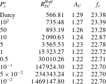
Table 3 shows the influence of
 $P_{r}^{\ast }$
on the onset of Hopf bifurcation, as predicted by linear stability theory, for
 $R_{S}=-240$
,
 $Le=10$
and
 $\unicode[STIX]{x1D700}=1$
. It is clear that the critical Rayleigh number,
 $R_{TC}^{Hopf}$
, at which a Hopf bifurcation occurs, increases considerably upon decreasing
 $P_{r}^{\ast }$
. In other words, a decrease of the modified Prandtl number results in a weakening of the convective flow and thus has a stabilizing effect.
Computed values of
 $R_{TC}^{Hopf}$
,
 $A_{C}$
and
 $f_{r}$
for
 $R_{S}=-240$
,
 $Le=10$
and
 $\unicode[STIX]{x1D700}=1$
.

6 Discussion
The results presented in this paper are focused on the effect of the form drag on classical double-diffusive convection, where mixed subcritical, overstable and stationary convection may occur. The most important new result and finding to report herein is the existence of a bistability phenomenon induced mainly by the form drag effect in Lapwood convective flow type through porous media at high Reynolds number.
In a binary convective unstable system, such as in Lapwood convection, and omitting the roll clockwise rotation direction, a bistability phenomenon arises when the system has two possible stable convective solutions occurring under the same conditions above the thresholds of stationary convection. One can be naturally initiated from the rest state and the other one must be triggered by a high nonlinear convective excitation. These two solutions have the same flow structure but different flow intensities, and exhibit different heat and mass transfer rates. These two solutions are usually connected by a third unstable solution, leading to an ‘S’ shape bifurcation near criticality.
Form drag effect on linear and nonlinear bifurcation behaviour in double-diffusive Lapwood convection within a horizontal porous layer.

Bifurcation diagram in terms of
 $\unicode[STIX]{x1D6F9}_{0}$
versus
 $R_{T}$
for
 $\unicode[STIX]{x1D711}=-0.1$
,
 $Le=5$
,
 $\unicode[STIX]{x1D700}=1$
and (a)
 $P_{r}^{\ast }=\infty$
, (b)
 $P_{r}^{\ast }=1$
and (c)
 $P_{r}^{\ast }=2$
; ——, analytical stable;


In the present study, the bistability phenomenon was found to occur within a region spanning between the onset of overstable and subcritical convection, at
 $R_{T}=\min (R_{TC}^{over},R_{TC}^{sub})$
, depending on the governing parameters, and the onset of supercritical convection,
 $R_{T}=R_{TC}^{sup}$
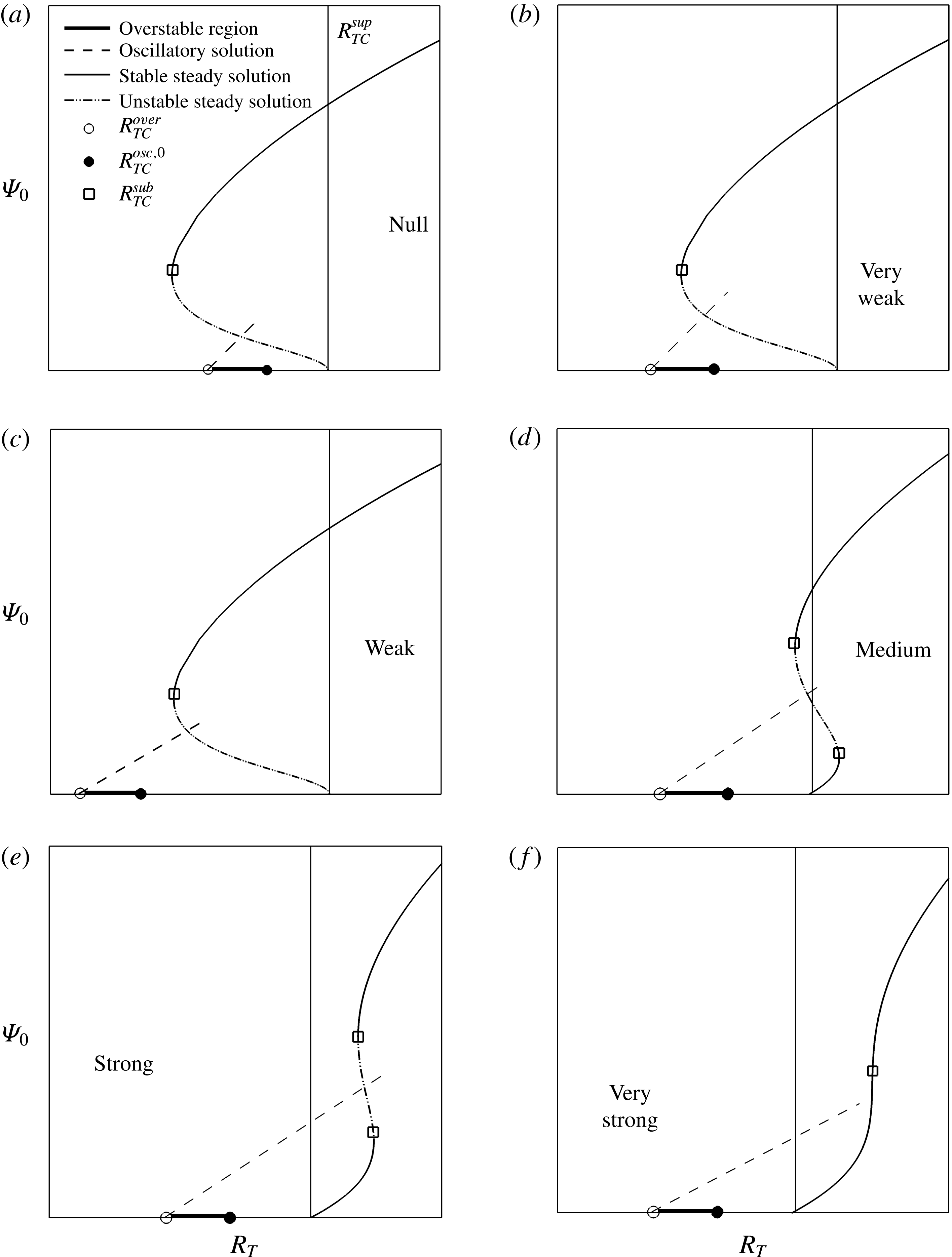
, or slightly beyond. For a situation where this phenomenon exists, the sequential bifurcation behaviour rated according to the form drag magnitude (from null to very strong) is exemplified in figure 3. The zone where the overstable regime occurs, according to the linear stability analysis, is indicated by a thick segment delineated by
 $R_{TC}^{over}$
and
 $R_{TC}^{osc,0}$
. To recall, in the overstable region, convection when initiated from the rest state is amplified in an oscillatory way. In figure 3(a), a typical Darcian subcritical bifurcation is depicted. The solid line refers to a stable steady-state solution, the dot-dot-dashed line refers to an unstable solution and the dashed line refers to a stable oscillatory solution. The onset of subcritical convection is designated by the saddle–node point depicted by a square empty symbol.
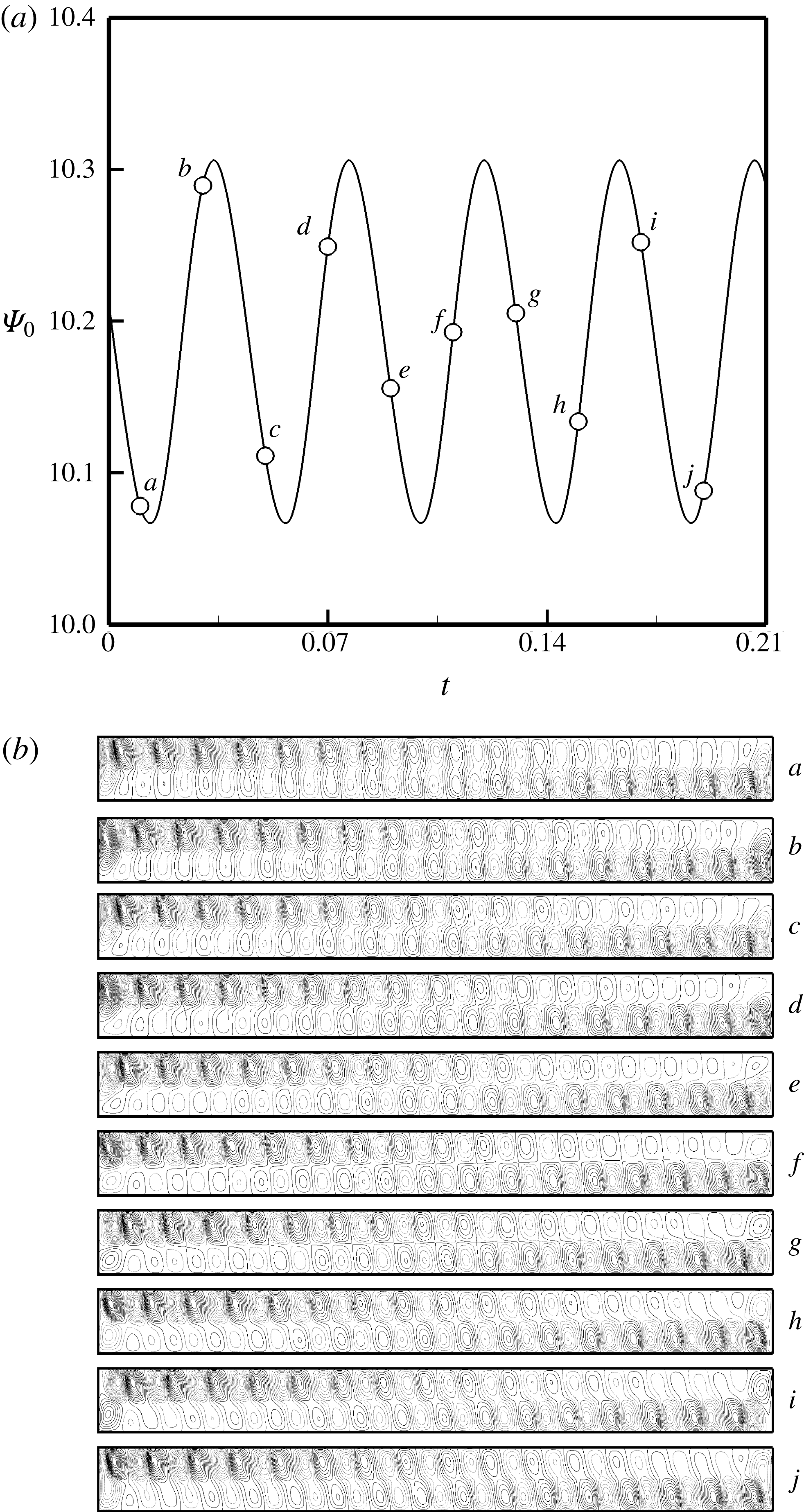
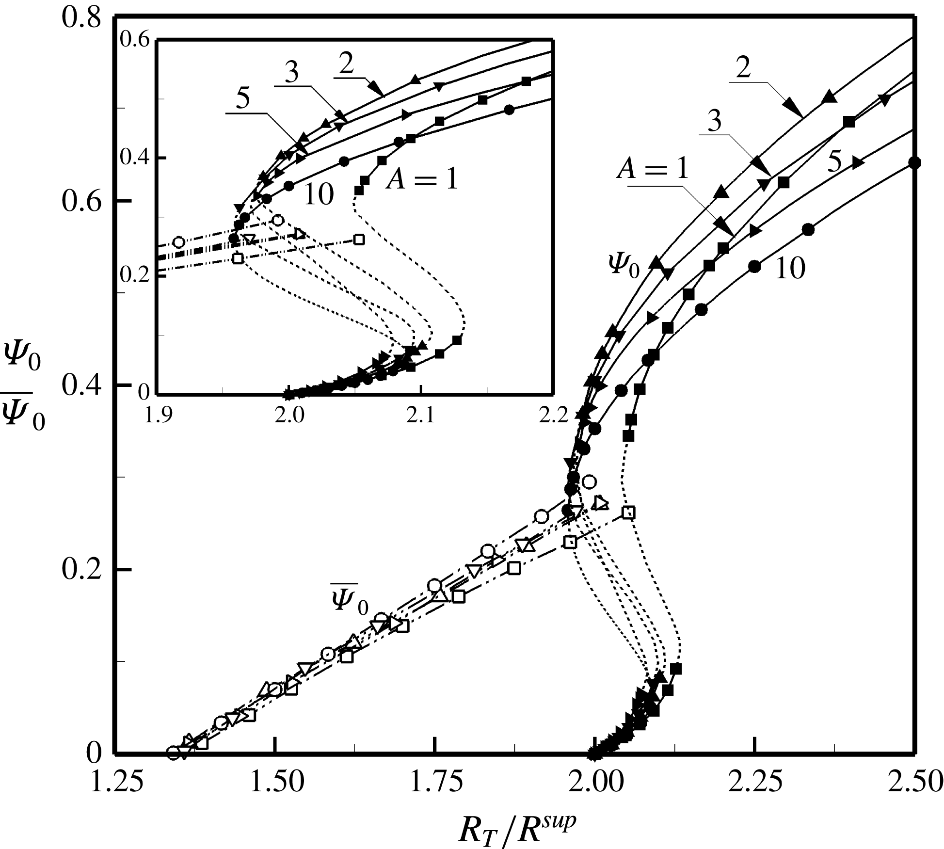
When transitioning from pure Darcy to dominant Dupuit convective regimes, the bifurcation behaviour undergoes a remarkable change according to the magnitude of the form drag coefficient. Figure 3(a) illustrates a typical Darcian bifurcation where the subcritical convection threshold is below the overstable one; this is denoted by a ‘null’ form drag effect. Increasing the form drag magnitude progressively, the threshold of subcritical convection increases continuously through the overstable region (‘very weak’) and then over along the stationary regime below the onset of the supercritical convection threshold (‘weak’ to ‘medium’ effect), leaving behind the possible occurrence of stationary or overstable flows. According to the medium effect situation, the single subcritical bifurcation is broken into a double subcritical bifurcation connected by an unstable branch. One bifurcation is forwards initiated at a saddle–node point below the threshold of supercritical convection, and the other one is backward but induced beyond that threshold. In this situation, a bistability regime occurs between the two thresholds. As the form drag effect becomes ‘strong’, the bistability region shrinks, and it disappears completely when the effect becomes ‘very strong’, as displayed in figure 3(f). Below the thresholds of supercritical convection, no matter what the form drag magnitude is, the developed convective flow is always sustained but oscillatory. More highlights on the bistability phenomenon are given in the following sections.
6.1 Shallow horizontal layer
$(A\gg 1)$

In this subsection, the effects of the governing parameters on the convective flows, as predicted by the present analytical solution, are compared with the numerical results obtained by solving the full governing equations. As discussed above, the governing parameters of the problem are the Rayleigh number
 $R_{T}$
, the buoyancy ratio
 $\unicode[STIX]{x1D711}$
, the Lewis number
 $Le$
, the normalized porosity
 $\unicode[STIX]{x1D700}$
and the modified Prandtl number
 $P_{r}^{\ast }$
.
Figure 4 exemplifies the effect of the modified Prandtl number,
 $P_{r}^{\ast }$
, on the onset of motion and the resulting convective flow in the present system. The form drag effect is proportional to
 $1/P_{r}^{\ast }$
. The bifurcation diagrams are presented in terms of the flow intensity,
 $\unicode[STIX]{x1D6F9}_{0}$
, the value of the stream function at the centre of the cavity, as a function of
 $R_{T}$
for
 $\unicode[STIX]{x1D711}=-0.1$
,
 $Le=5$
and
 $\unicode[STIX]{x1D700}=1$
. The curves depicted in the graphs are the predictions of the present analytical/numerical nonlinear theories. The solid lines correspond to stable branches and the dot-dot-dashed lines to unstable ones. The numerical solutions of the full governing equations, obtained for
 $A=10$
, are shown by solid circles. A good agreement is observed between these two nonlinear theory results. For the values of the governing parameters considered here, the critical Rayleigh numbers for the onset of motion, as predicted by (4.22), are given by
 $R_{TC}^{sup}=24$
,
 $R_{TC}^{over}=16$
and
 $R_{TC}^{osc,0}=20.53$
. These critical Rayleigh numbers are not affected by the form drag since they correspond to onsets of motion occurring from the rest state. It is well known that the flow circulation in the layer can be indifferently clockwise or counterclockwise. Since the results are symmetrical, only the counterclockwise solutions
 $(\unicode[STIX]{x1D6F9}_{0}>0)$
are depicted in all of the bifurcation curves presented in this paper.
The results presented in figure 4(a) are obtained for
 $P_{r}^{\ast }\rightarrow \infty$
, i.e. in the absence of form drag effects. The resulting bifurcation curve is consistent with the behaviour reported in the past by Mamou & Vasseur (Reference Mamou and Vasseur1999) and Bahloul et al. (Reference Bahloul, Vasseur and Robillard2007), while considering double-diffusive and Soret-induced convection in a porous layer modelled according to Darcy’s law. The onset of motion is characterized by a transition from the rest state through finite amplitude convection
 $(\unicode[STIX]{x1D6F9}_{0}\neq 0)$
, i.e. nonlinear instabilities. This transition occurs at a subcritical Rayleigh number of
 $R_{TC}^{sub}=15.63$
, which is well below the supercritical Rayleigh number of
 $R_{TC}^{sup}=24$
. At this threshold, subcritical bifurcation occurs only when the buoyancy forces induced by the thermal and solutal contributions are opposing each other and when the stabilizing agent is the slower diffusing component
 $(Le>1)$
. In the graph, the solution depicted by the solid line (thermal branch), referred to as the stable solution, is confirmed by the numerical results depicted by black circles. This is not the case for the dot-dot-dashed line (solutal branch), connecting the subcritical and supercritical Rayleigh numbers, which corresponds to an unstable solution. The thermal and the solutal lines are connected to each other at a saddle–node bifurcation. In general, the numerical results presented in figure 4(a) indicate that, below the subcritical Rayleigh number (region I), the rest state prevails. In region (II), delineated by
 $R_{TC}^{sub}\leqslant R_{T}\leqslant R_{TC}^{over}$
, parallel flow theory predicts the existence of two solutions (one stable and the other one not). In region (III), delimited by
 $R_{TC}^{over}\leqslant R_{T}\leqslant R_{TC}^{osc,0}$
, starting with the conduction state as initial conditions, the numerical results indicate that for
 $R_{T}=16.1$
the flow is oscillatory. The result is presented in the graph, by circle symbols, in terms of the root mean square of the stream function,
 $\overline{\unicode[STIX]{x1D6F9}}_{0}$
. Upon increasing the Rayleigh number step by step and using the previous results as initial conditions, the oscillating flow branch
 $\overline{\unicode[STIX]{x1D6F9}}_{0}$
can be sustained up to
 $R_{T}=16.9$
. Above this Rayleigh number, the solution bifurcates directly towards the steady convective motion predicted by parallel flow theory. Numerically, it was found that upon increasing (decreasing) the Rayleigh number and starting the computations with a conductive state (finite amplitude convection) the resulting solution follows the hysteresis loop depicted by the arrow paths depicted on the graphs.
The results presented in figure 4(b) are obtained for a relatively small value of the modified Prandtl number, namely
 $P_{r}^{\ast }=1$
, for which the form drag effect is significant. As already mentioned, the critical Rayleigh numbers for the onset of motion from the rest state (
 $R_{TC}^{over}$
,
 $R_{TC}^{osc,0}$
,
 $R_{TC}^{sup}$
) are not affected by the form drag effect. Thus, the minimum critical Rayleigh number for the onset of linear motion is the overstable Rayleigh number
 $R_{TC}^{over}=16$
, such that below this value, zone (I), the system remains at rest, as indicated by the numerical results presented in the graph. Above this value, similarly to the results obtained in figure 4(a), for
 $R_{T}>R_{TC}^{over}$
the numerical results reveal the existence of an oscillating flow branch,
 $\overline{\unicode[STIX]{x1D6F9}}_{0}$
, over the range
 $16.2\leqslant R_{T}\leqslant 28.5$
. The resulting type of oscillating flow, in zone (II), is illustrated in figure 4(b) for the particular case
 $R_{T}=18$
in terms of the time history of
 $\unicode[STIX]{x1D6F9}_{0}$
for a few cycles. It is found that the oscillating branch also exists in zone (III), delineated by
 $R_{TC}^{osc,0}\leqslant R_{T}\leqslant R_{TC}^{sup}$
, as exemplified by the results obtained for
 $R_{T}=22$
. The oscillatory solution branch is also observed to extend beyond
 $R_{T}=R_{TC}^{sup}$
, where it bifurcates toward the steady state solution branch. The solid line in zone (IV) is the prediction of nonlinear parallel flow theory. It is observed that the onset of steady motion is now not subcritical, compared with figure 4(a) for Darcy’s law, but rather supercritical. The resulting pitchfork type bifurcation, characterized by a transition from the rest state
 $(\unicode[STIX]{x1D6F9}_{0}=0)$
to a convective regime, takes place at a supercritical Rayleigh number of
 $R_{TC}^{sup}=24$
. Upon increasing the Rayleigh number above this critical value, a good agreement is observed between the analytical and numerical results.
Two possible time histories of the stream function intensity
 $\unicode[STIX]{x1D6F9}_{0}$
and the flow structure for
 $\unicode[STIX]{x1D711}=-0.1$
,
 $Le=5$
,
 $P_{r}^{\ast }=2$
and
 $\unicode[STIX]{x1D700}=1$
: (a)
 $R_{T}=18$
(zone II), (b)
 $R_{T}=22$
(zone III).

The case
 $P_{r}^{\ast }=2$
, which is an intermediate value of the modified Prandtl number between those considered above, is depicted in figure 4(c). The bifurcation diagram is now characterized by six different zones. In particular, zones (I) and (II), delineated by
 $R_{TC}^{over}$
and
 $R_{TC}^{osc,0}$
, are the same as those discussed above, for
 $P_{r}^{\ast }=1$
. Thus, the rest state prevails in zone (I), while for
 $R_{T}>R_{TC}^{over}$
the flow is found to be oscillatory. This flow regime gives rise to a branch corresponding to the numerical results obtained for
 $\overline{\unicode[STIX]{x1D6F9}}_{0}$
versus
 $R_{T}$
. It is found that the oscillating branch can be maintained up to
 $R_{T}=23.9$
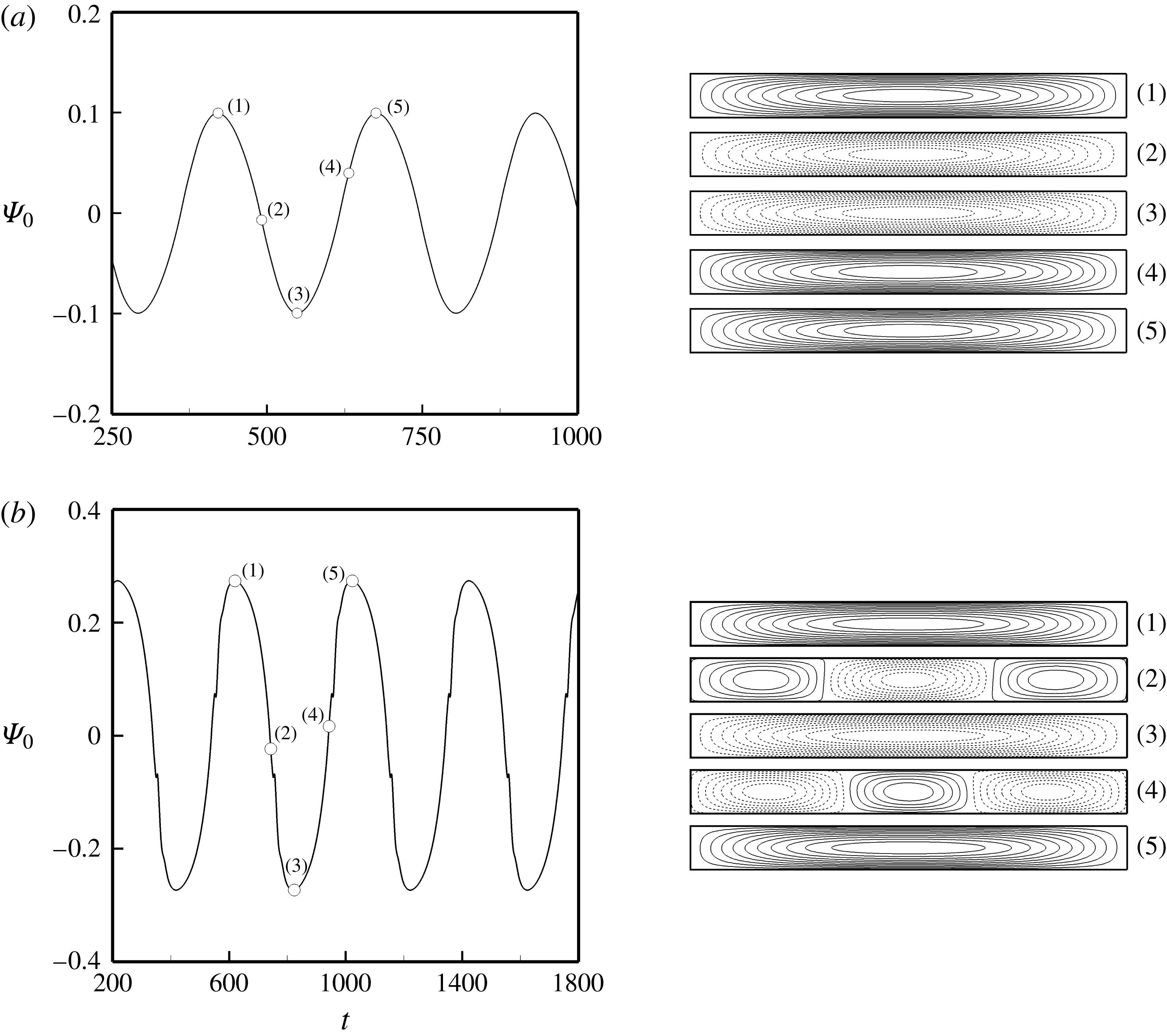
, above which the numerical solution bifurcates towards a steady finite amplitude convective regime. Figure 5(a) illustrates the results obtained for
 $R_{T}=18$
, zone (II), in terms of the variation of the stream function
 $\unicode[STIX]{x1D6F9}_{0}$
in time and selected streamline patterns during a period. The flow structure consists of a unicellular cell filling up the entire cavity. An overturning of the flow from counterclockwise to clockwise circulation and vice versa is observed. The bifurcation curve, predicted by parallel flow theory, indicates the onset of motion occurring now at a subcritical Rayleigh number of
 $R_{TC}^{sub}=23.51$
. Thus, zone (III) in the graph is now confined in the range
 $R_{TC}^{osc,0}\leqslant R_{T}\leqslant R_{TC}^{sub}$
. Figure 5(b) illustrates the results obtained in this region, for
 $R_{T}=22$
. The strength of the resulting oscillating circulation is found to be naturally higher than that reported in zone (II) and the corresponding flow structure is more complex. At time
 $t=620$
, the flow pattern consists of a counterclockwise unicellular circulation. As time increases, this unicellular structure breaks up to give rise to a central clockwise circulation and two small counterclockwise rotating eddies, localized near the end regions of the cavity. These two eddies vanish gradually, giving rise to a weak unicellular clockwise circulation in the layer, as can be seen from the results obtained at
 $t=840$
. As time progresses further, the flow pattern consists of a counterclockwise circulating cell in the central part of the system and two clockwise eddies near the end regions. At time
 $t=1020$
, the unicellular counterclockwise circulation observed at
 $t=620$
is recovered. The whole process is repeated during each time period. This oscillatory behaviour and the flow patterns could be different when the layer aspect ratio is varied. The results, predicted by the present parallel flow model, are now discussed. The resulting bifurcation curve is seen to be quite particular. A bird’s-eye view of the graph indicates the existence of two stable different branches, depicted by solid lines. The upper one, starting at
 $R_{TC}^{sub}$
, is the standard branch observed in subcritical bifurcations, as exemplified, for instance, in figure 4(a). On the other hand, the lower stable branch, which starts at
 $R_{TC}^{sup}=24$
, corresponds to a supercritical bifurcation similar to that discussed in figure 4(b). However, it is observed that this latter exists only in the range
 $R_{TC}^{sup}\leqslant R_{T}\leqslant R_{TC}^{tur}$
, where
 $R_{TC}^{tur}=25.08$
corresponds to a turning saddle–node point. The two stable branches are connected with each other by an unstable branch, shown as a dot-dot-dashed line. This is a typical bistability bifurcation. Numerical confirmation of the analytical solution is also presented in the graph and here again the agreement is excellent. Starting the numerical procedure with the rest state as initial conditions, it was found that, upon increasing the Rayleigh number above
 $R_{TC}^{sub}=23.51$
, the resulting solution follows the hysteresis loop depicted by arrows in the zoom included in figure 4(c). Thus, for
 $R_{T}\geqslant R_{TC}^{tur}$
, zone (VI), only the upper branch exists and it is seen that, as expected, upon increasing
 $R_{T}$
the strength of the convection is promoted monotonically. Such a steady solution can be maintained up to a critical Rayleigh number of
 $R_{TC}^{Hopf}$
, above which a Hopf bifurcation occurs and the flow becomes unsteady. Hopf bifurcation will be covered in the following section. On the other hand, upon decreasing the Rayleigh number below
 $R_{TC}^{tur}$
, one must now consider two distinct zones. Zone (V) is characterized by the existence for a given Rayleigh number of three possible different solutions (two stable and one unstable). Region (V), which is demarcated by
 $R_{TC}^{sup}\leqslant R_{T}\leqslant R_{TC}^{tur}$
, is the cradle where a bistability phenomenon occurs leading to the existence of two distinct finite amplitude solutions between two forward and backward subcritical bifurcations, even though it happens beyond the thresholds of supercritical convection. Within this region, two lower and upper stable convective branches were obtained and connected by a third unstable branch.
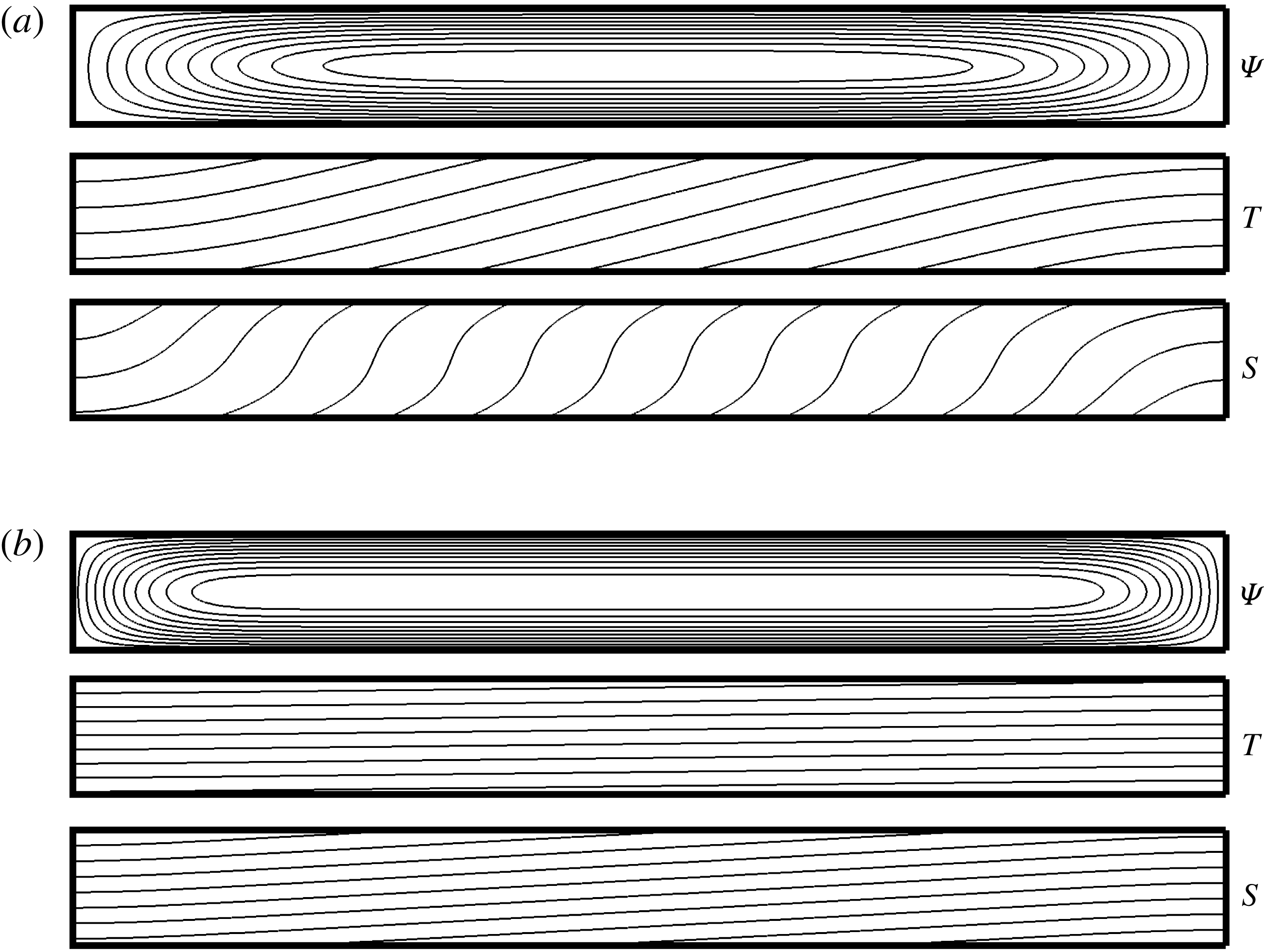
Figure 6(a,b) illustrates the streamlines, isotherms and isoconcentrates obtained numerically in the bistability convection zone, for
 $R_{T}=24.5$
. Appropriate initial conditions had to be specified to simulate the two different stable solutions. Thus, to help in bifurcating towards the desired solution, the analytical solution was used as initial condition. For the upper branch, the lower branch can be obtained naturally when departing from the rest state. The upper-branch flow patterns are shown in figure 6(a) and the lower-branch patterns are displayed in figure 6(b). Naturally, it has not been possible to confirm numerically the third unstable solution predicted by the analytical model.
Contours of stream (top), temperature (middle) and concentration (bottom) for
 $R_{T}=24.5$
,
 $P_{r}^{\ast }=2$
,
 $\unicode[STIX]{x1D711}=-0.1$
,
 $Le=10$
and
 $\unicode[STIX]{x1D700}=1$
; (a)
 $\unicode[STIX]{x1D6F9}_{0}=0.394$
,
 $Nu=1.063$
,
 $Sh=2.182$
; (b)
 $\unicode[STIX]{x1D6F9}_{0}=0.016$
,
 $Nu=1.000$
,
 $Sh=1.003$
.

Bifurcation diagram as a function of
 $R_{T}$
and
 $P_{r}^{\ast }$
for
 $\unicode[STIX]{x1D711}=-0.1$
,
 $Le=5$
and
 $\unicode[STIX]{x1D700}=1$
; (a) flow intensity
 $\unicode[STIX]{x1D6F9}_{0}$
, (b) Nusselt number
 $Nu$
and (c) Sherwood number
 $Sh$
; ——, analytical stable;


A more complete view of the effects of
 $P_{r}^{\ast }$
and
 $R_{T}$
on
 $\unicode[STIX]{x1D6F9}_{0}$
,
 $Nu$
and
 $Sh$
is presented in figure 7(a–c) for
 $\unicode[STIX]{x1D711}=-0.1$
,
 $Le=5$
and
 $\unicode[STIX]{x1D700}=1$
. Results are obtained for values of the modified Prandtl number ranging between
 $P_{r}^{\ast }=\infty$
(Darcy) and 1. In general, it is seen from figure 7(a) that, for a given Rayleigh number, a decrease in the form drag parameter reduces the strength of the convective motion in the layer considerably. This is due to the fact that decrease of
 $P_{r}^{\ast }$
results in an increase of the form drag. Consequently, as can be observed from figure 7(b,c), both the heat and the mass transfer rates are considerably inhibited with a decrease of the modified Prandtl number. The plots also clearly show the effect of
 $P_{r}^{\ast }$
on the existence of the different types of bifurcation curves discussed in figure 4. For the set of governing parameters considered here, it is predicted by the analytical model that the bifurcation is subcritical provided that
 $P_{r}^{\ast }>1.85$
, as depicted in figure 8(a) for
 $P_{r}^{\ast }=2$
. The resulting bifurcation curve is characterized by an upper subcritical stable branch existing for
 $R_{T}\geqslant R_{TC}^{sub}=23.5$
. Furthermore, due to the form drag effect, the graph also indicates the existence of a supercritical stable branch extending in the range
 $R_{TC}^{sup}=24\leqslant R_{T}\leqslant R_{TC}^{tur}=25.1$
. Both
 $R_{TC}^{sub}$
and
 $R_{TC}^{tur}$
are connected to each other by an unstable branch depicted by a dot-dot-dashed line. Upon decreasing the value of
 $P_{r}^{\ast }$
, the onset of motion remains subcritical down to
 $P_{r}^{\ast }=1.85$
, at which point the condition
 $R_{TC}^{sub}=R_{TC}^{sup}=24$
is reached, as illustrated in figure 8(b). For
 $P_{r}^{\ast }\leqslant 1.85$
, it is seen from figure 8(b,c) that the onset of motion is now supercritical (
 $R_{TC}^{sub}\geqslant R_{TC}^{sup}$
). Thus, as exemplified in figure 8(c) for
 $P_{r}^{\ast }=1.5$
, it is noticed that the subcritical Rayleigh number
 $R_{TC}^{sub}$
becomes greater than
 $R_{TC}^{sup}$
, such that it degenerates into a second turning point
 $R_{TC}^{sub}$
. The bifurcation curve is now characterized by two turning points,
 $R_{TC}^{sub}=25.4$
and
 $R_{TC}^{tur}=25.9$
. It is noted from figure 8(a–c) that, in the range
 $R_{TC}^{sup}(R_{TC}^{sub})\leqslant R_{T}\leqslant R_{TC}^{tur}$
, three different solutions (two stable and one unstable) are possible for a given
 $R_{T}$
, confirming the existence of the bistability phenomenon discussed above. Finally, the results presented in figure 8(d) for
 $P_{r}^{\ast }=1.3$
indicate that the condition
 $R_{TC}^{tur}=R_{TC}^{sub}=26.5$
is reached. As a result, for
 $P_{r}^{\ast }\leqslant 1.3$
, the analytical model predicts that, for a given Rayleigh number
 $R_{T}>R_{TC}^{sup}$
, the resulting supercritical bifurcation curves are now single valued. A stability diagram is illustrated in figure 8(e), where the bistability region is delineated by the hatched area.
Bifurcation diagram in terms of
 $\unicode[STIX]{x1D6F9}_{0}$
versus
 $R_{T}$
for
 $\unicode[STIX]{x1D711}=-0.1$
and
 $Le=5$
; (a)
 $P_{r}^{\ast }=2$
, (b)
 $P_{r}^{\ast }=1.85$
, (c)
 $P_{r}^{\ast }=1.5$
and (d)
 $P_{r}^{\ast }=1.3$
; ——, analytical stable;


Analytical results obtained for
 $P_{r}^{\ast }=2$
,
 $Le=5$
and
 $\unicode[STIX]{x1D700}=1$
: (a) bifurcation diagram in terms of
 $\unicode[STIX]{x1D6F9}_{0}$
versus
 $R_{T}$
, (b) critical Rayleigh number
 $R_{TC}$
versus
 $\unicode[STIX]{x1D711}$
.

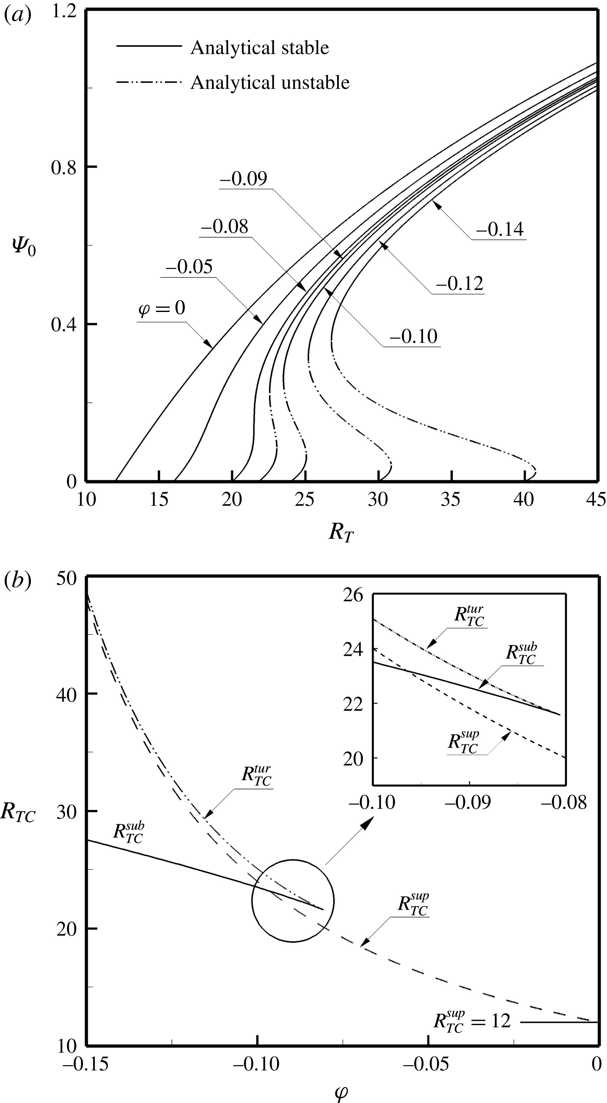
Figure 9(a) shows typical bifurcation diagrams for
 $\unicode[STIX]{x1D6F9}_{0}$
as a function of
 $R_{T}$
and
 $\unicode[STIX]{x1D711}$
for
 $P_{r}^{\ast }=2$
,
 $Le=5$
and
 $\unicode[STIX]{x1D700}=1$
. The curve obtained for
 $\unicode[STIX]{x1D711}=0$
corresponds to convection induced solely by the thermal effect. It gives rise to a pitchfork bifurcation occurring at a supercritical Rayleigh number of
 $R_{TC}^{sup}=12$
. The way in which this supercritical bifurcation is affected upon decreasing the value of the buoyancy ratio is illustrated in the graph. In fact, the evolution of the bifurcation curves with the buoyancy ratio is quite similar to that discussed in figure 8(a–d) while studying the effect of
 $P_{r}^{\ast }$
. Figure 9(b) shows the variation of the critical Rayleigh numbers
 $R_{TC}^{sup}$
,
 $R_{TC}^{sub}$
and
 $R_{TC}^{tur}$
with
 $\unicode[STIX]{x1D711}$
. The graph indicates that in the range
 $-0.15\leqslant \unicode[STIX]{x1D711}\leqslant -0.096$
, the subcritical Rayleigh number is the lower critical Rayleigh number
 $(R_{TC}^{sub}<R_{TC}^{sup}<R_{TC}^{tur})$
, such that the onset of motion is subcritical, as exemplified in figure 8(a). At
 $\unicode[STIX]{x1D711}=-0.096$
, it is found that
 $R_{TC}^{sub}=R_{TC}^{sup}=23.19$
, this situation being similar to that depicted in figure 8(b). Upon keeping on decreasing the value of the buoyancy ratio, it is observed that, in the range
 $-0.096\leqslant \unicode[STIX]{x1D711}\leqslant -0.081$
, the bifurcation curve consists of a lower supercritical branch extending in the range
 $R_{TC}^{sup}\leqslant R_{T}\leqslant R_{TC}^{tur}$
and an upper branch that exists for the condition
 $R_{T}\geqslant R_{TC}^{sub}$
, as exemplified in figure 8(c). The subcritical branch has thus degenerated into a branch corresponding to the critical Rayleigh number
 $R_{TC}^{sub}$
. The results obtained at
 $\unicode[STIX]{x1D711}=-0.081$
, for which
 $R_{TC}^{tur}=R_{TC}^{sub}=21.58$
, are similar to those depicted in figure 8(d), i.e. the two turning point branches merge. For
 $-0.081\leqslant \unicode[STIX]{x1D711}\leqslant 0$
, the only existing critical Rayleigh number is the supercritical one,
 $R_{TC}^{sup}$
.
(a) Subcritical Rayleigh number
 $R_{TC}^{sub}$
as a function of
 $P_{r}^{\ast }$
and
 $Le$
for
 $\unicode[STIX]{x1D711}=-0.1$
. (b) Bifurcation diagram in terms of
 $\unicode[STIX]{x1D6F9}_{0}$
as a function of
 $R_{T}$
and
 $P_{r}^{\ast }$
for
 $\unicode[STIX]{x1D711}=-0.1$
,
 $Le=15$
and
 $\unicode[STIX]{x1D700}=1$
; ——, analytical stable;


The subcritical Rayleigh number
 $R_{TC}^{sub}$
is plotted in figure 10(a) as a function of
 $P_{r}^{\ast }$
and various values of the Lewis number, for the case
 $\unicode[STIX]{x1D711}=-0.1$
. For larger values of the modified Prandtl number
 $(P_{r}^{\ast }\rightarrow \infty )$
, the results predicted by Darcy’s model, equation (4.23), are recovered, as depicted in the small inset included in the graph. Thus, as
 $Le\rightarrow \infty$
, the solute concentration is almost uniform in the system, except in very thin layers near the horizontal boundaries. Consequently, the onset of convection approaches asymptotically the criterion for the onset of convection in a porous layer subjected solely to constant heat fluxes (i.e.
 $R_{TC}^{sub}\rightarrow R_{TC}^{sup}=12$
). Upon decreasing the Lewis number progressively,
 $R_{TC}^{sub}$
first increases sharply, up to a maximum,
 $R_{TC}^{sub}=16$
at
 $Le=3.22$
, and then decreases monotonically. It is observed that below
 $Le=2.16$
, subcritical convection is not possible. This follows from the fact that when the Lewis number is small enough, the mass transfer process across the porous layer is ruled by pure diffusion. The onset of motion is then supercritical, occurring at a Rayleigh number of
 $R_{TC}^{sup}=15.3$
, as predicted by (4.22). Upon keeping on decreasing the Lewis number further, it is seen that the supercritical Rayleigh number tends asymptotically towards
 $R_{TC}^{sup}=12$
as
 $Le\rightarrow 0$
. The effect of the modified Prandtl number on the subcritical Rayleigh number is clearly illustrated in the graph. As already mentioned, a decrease of
 $P_{r}^{\ast }$
annihilates the strength of the convective motion in the layer. Thus, for a given Lewis number, it is found that the value of
 $R_{TC}^{sub}$
, at which convection occurs, increases considerably upon decreasing
 $P_{r}^{\ast }$
. For instance, for
 $Le=10^{3}$
, it is found that the subcritical Rayleigh number increases from
 $R_{TC}^{sub}=12.25$
for
 $P_{r}^{\ast }=10^{3}$
to
 $R_{TC}^{sub}=28$
for
 $P_{r}^{\ast }=10^{-1}$
. Naturally, for the lower values of the Lewis number presented in the graph, subcritical convection is not always possible as the modified Prandtl number is decreased. Hence, for
 $Le=3(5)$
, the onset of motion is supercritical for
 $P_{r}^{\ast }\leqslant 14(1.85)$
. Another view of the effect of the modified Prandtl number is illustrated in figure 10(b). The results obtained in terms of
 $\unicode[STIX]{x1D6F9}_{0}$
as a function of
 $R_{T}$
and
 $P_{r}^{\ast }$
, for
 $\unicode[STIX]{x1D711}=-0.1$
and
 $Le=15$
, are found to be different from those discussed in figure 7(a) for
 $Le=5$
. Thus, independently of the value of
 $P_{r}^{\ast }$
, the analytical solution indicates that the subcritical bifurcation curves consist of upper stable branches connected with lower unstable branches. The latter are seen to tend asymptotically towards the supercritical Rayleigh number
 $R_{TC}^{sup}\rightarrow \infty$
. In fact, for the particular Lewis number considered here, onset of supercritical convection is possible only for a negative value of the Rayleigh number, namely
 $R_{TC}^{sup}=-24$
, as predicted by (4.22). A negative value of
 $R_{T}$
corresponds to the case of a layer heated from the top. Decrease of the value of the Rayleigh number below this critical value yields the pitchfork bifurcation curves depicted in the graph. Although the strength of the resulting convective motions
 $\unicode[STIX]{x1D6F9}_{0}$
is very small, the enlargement depicted in figure 10(b) shows that the agreement between the analytical model and the numerical code is very good. For a given value of the form drag coefficient, it is seen that the rest state prevails in the range
 $-24\leqslant R_{T}\leqslant R_{TC}^{sub}(P_{r}^{\ast })$
.
Figure 11(a) shows the influence of the form drag coefficient on the thresholds of bifurcations
 $(R_{TC}^{Hopf},R_{TC}^{sub},R_{TC}^{sup},R_{TC}^{over},R_{TC}^{osc,0})$
for
 $R_{S}=-240$
,
 $Le=10$
and
 $\unicode[STIX]{x1D700}=0.2$
. According to (4.22), the onsets of motion from the rest state are given by
 $R_{TC}^{over}=138$
,
 $R_{TC}^{osc,0}=180$
and
 $R_{TC}^{sup}=252$
, these values being independent of
 $P_{r}^{\ast }$
. As expected, the graph indicates that the onset of Hopf bifurcation,
 $R_{TC}^{Hopf}$
, decreases sharply upon increasing the value of the form drag parameter. It follows that the steady parallel flow is destabilized earlier with an increase of
 $P_{r}^{\ast }$
. A similar trend is observed for the evolution of the subcritical Rayleigh number,
 $R_{TC}^{sub}$
, with the form drag coefficient. In both cases, for sufficiently large values of
 $P_{r}^{\ast }$
, the Darcy limits represented by dashed lines are reached asymptotically. It is also observed that, in the range
 $0.12\leqslant P_{r}^{\ast }\leqslant 10^{3}$
, the minimum critical Rayleigh number for the onset of motion is the subcritical one. However, for
 $P_{r}^{\ast }\leqslant 0.12$
, linear stability theory predicts that convection is possible when
 $R_{T}\geqslant R_{TC}^{over}$
, the overstable critical Rayleigh number. Figure 11(b) illustrates the effect of
 $P_{r}^{\ast }$
on the wavelength
 $A_{C}$
of the incipient flow structure at the onset of Hopf bifurcation. It is found that the wavelength (frequency) decreases (increases) monotonically from
 $A_{C}=1.35$
(
 $f_{r}=21$
), in the pure Darcy regime, towards
 $A_{C}=1.22$
(
 $f_{r}=22.67$
), in the pure Dupuit regime. The form drag effects on these two parameters are thus relatively weak.
Form drag effect for
 $R_{S}=-240$
,
 $Le=10$
,
 $Pr^{\ast }=10$
, and
 $\unicode[STIX]{x1D700}=0.2$
on (a) the thresholds of convection
 $R_{TC}$
and (b) the critical wavelength
 $A_{C}$
and oscillatory frequency
 $f_{r}$
.

Bifurcation diagram in terms of
 $\unicode[STIX]{x1D6F9}_{0}$
versus
 $R_{T}$
for
 $R_{S}=-240$
,
 $Le=10$
,
 $Pr^{\ast }=10$
, and
 $\unicode[STIX]{x1D700}=0.2$
; ——, analytical stable;


Figure 12 exemplifies the effects of the thermal Rayleigh number,
 $R_{T}$
, on the flow intensity,
 $\unicode[STIX]{x1D6F9}_{0}$
, for the case where
 $R_{S}=-240$
,
 $P_{r}^{\ast }=10$
,
 $Le=10$
and
 $\unicode[STIX]{x1D700}=0.2$
. The numerical results obtained for a cavity with an aspect ratio of
 $A=20$
are observed to be in excellent agreement with the prediction of the parallel flow model. According to (4.22), the critical Rayleigh numbers for the onset of motion from the rest state are given by
 $R_{TC}^{over}=138$
,
 $R_{TC}^{osc,0}=180$
and
 $R_{TC}^{sup}=252$
. The onset of oscillating motion, predicted by the numerical procedure described in § 3, occurs at
 $R_{TC}^{Hopf}=1967$
, while the onset of subcritical convection predicted by the nonlinear parallel flow approximation is
 $R_{TC}^{sub}=29$
. In the graph, zones (I)–(V) are equivalent to those defined in figure 4(a), while in zone (VI), for which
 $R_{T}\geqslant R_{TC}^{Hopf}$
, the convective flow is oscillating. This point is confirmed by the numerical results obtained for
 $R_{T}=2200$
, 3000 and 4000. The empty circles presented in the graph correspond to the resulting time-averaged values of
 $\unicode[STIX]{x1D6F9}_{0}$
obtained by the numerical code. The time evolution of the flow intensity,
 $\unicode[STIX]{x1D6F9}_{0}$
, obtained for
 $R_{T}=2200$
, just above the critical Rayleigh number for Hopf bifurcation predicted by linear stability theory
 $(R_{TC}^{Hopf}=1967)$
, is depicted in figure 13(a). The resulting oscillatory flow is found to be simply periodic. Snapshots of the perturbations of the stream function (obtained from subtracting the time-averaged solution from the time-accurate one) at different time steps shown in figure 13(a) are presented in figure 13(b). The numerical results indicate that the critical wavelength and the oscillation frequency are given by
 $A_{C}=1.25$
and
 $f_{r}=23.15$
respectively, which are close to the values
 $A_{C}=1.24$
and
 $f_{r}=22.30$
predicted by linear stability theory. At the onset of Hopf bifurcation, as predicted by the linear stability analysis, there exist two symmetrical solutions at the same circular frequency
 $p_{i}$
(imaginary part of
 $p$
) but with opposite signs. The negative and positive signs indicate the existence of travelling waves in the horizontal direction in both ways, as demonstrated by the full numerical solution presented in figure 13(b) and by the supplementary movies (available at https://doi.org/10.1017/jfm.2016.787). The incipient perturbation flow patterns, obtained by the linear stability analysis, are illustrated in figure 11(b), and once superposed they appear to be similar to those obtained numerically in figure 13(b).
(a) Time history of the stream function
 $\unicode[STIX]{x1D6F9}_{0}$
as predicted by the numerical solution and (b) snapshots of the perturbations of the stream function
 $\unicode[STIX]{x1D6F9}_{p}$
corresponding to selected points, for
 $R_{T}=2200$
,
 $R_{S}=-240$
,
 $Le=10$
,
 $Pr^{\ast }=10$
,
 $A=20$
and
 $\unicode[STIX]{x1D700}=0.2$
. Animations of the stream function, temperature and solute concentration perturbations can be seen in the supplementary movies.

6.2 Square cavity
$(A=1)$

In this section, we consider the case of a square cavity subject to vertical temperature and concentration gradients. The two vertical walls of the cavity are impermeable and adiabatic, while Dirichlet or Neumann boundary conditions on temperature and solute are imposed on the horizontal walls. For this situation, an analytical model is not available, such that all of the results presented here are the predictions of the numerical code discussed in § 3.
Bifurcation diagram in terms of
 $\unicode[STIX]{x1D6F9}_{0}$
as a function of
 $R_{T}$
and
 $P_{r}^{\ast }$
for
 $A=1$
,
 $\unicode[STIX]{x1D711}=-0.1$
,
 $Le=5$
and
 $\unicode[STIX]{x1D700}=1$
; (a)
 $P_{r}^{\ast }=\infty$
–1; (b)
 $P_{r}^{\ast }=2$
;


 $R_{T}=48$
,
 $P_{r}^{\ast }=2$
:
 $\unicode[STIX]{x1D6F9}_{0}=0.433$
,
 $Nu_{m}=1.040$
,
 $Sh_{m}=1.779$
(upper solution). (d) Contours of stream (left), temperature (middle) and concentration (right) for
 $R_{T}=48$
,
 $P_{r}^{\ast }=2$
:
 $\unicode[STIX]{x1D6F9}_{0}=0.047$
,
 $Nu_{m}=1.000$
,
 $Sh_{m}=1.013$
(lower solution). (Neumann boundary conditions.)

Figure 14(a–d) shows typical results obtained for the case of a square cavity heated and salted from the bottom by constant fluxes. Figure 14(a) illustrates the bifurcation curve, depicting the effects of the Rayleigh number,
 $R_{T}$
, and the modified Prandtl number,
 $P_{r}^{\ast }$
, on the flow intensity,
 $\unicode[STIX]{x1D6F9}_{0}$
, for the case
 $\unicode[STIX]{x1D711}=-0.1$
,
 $Le=5$
and
 $\unicode[STIX]{x1D700}=1$
. The solid lines in the graph are obtained by a curve fitting of the numerical data, while the dot-dot-dashed lines are manually guessed predictions (artistic) based on the results obtained for the shallow layer. A bird’s-eye view of the graph indicates that the results are quantitatively similar to those obtained in the previous section for a high-aspect-ratio layer. Thus, upon decreasing the value of the Prandtl number from
 $P_{r}^{\ast }=\infty$
to 1, it is seen that the bifurcation curves evolve from a subcritical behaviour to a supercritical one. For intermediates values of the modified Prandtl number, the bifurcation curves indicate the occurrence of stable supercritical and subcritical branches connected by an unstable one. This point is exemplified by the curve for
 $P_{r}^{\ast }=2$
depicted in figure 14(b), showing again the region where bistability convection occurs. For this situation, two finite and distinct convective solutions are possible for a given range of the Rayleigh number depending upon the governing parameters of the problem. This point is illustrated in figure 14(c,d), showing the streamlines, isotherms and isoconcentrates obtained for
 $R_{T}=48$
. The solution presented in figure 14(d), which corresponds to the lower branch, is obtained starting the numerical calculations using the rest state as initial conditions. However, the solution corresponding to the upper branch, figure 14(c), can be obtained only upon following the hysteresis path depicted on the curve for
 $P_{r}^{\ast }=2$
. Figure 15 shows typical results obtained for a cavity subject to Dirichlet type thermal and solutal boundary conditions. The governing parameters considered here are the same as those for figure 14. It is clear that the existence of dual solutions is also obtained, as depicted by the bifurcation curve obtained, for instance, for
 $P_{r}^{\ast }=5$
.
Bifurcation diagram in terms of
 $\unicode[STIX]{x1D6F9}_{0}$
as a function of
 $R_{T}$
and
 $P_{r}^{\ast }$
for
 $A=1$
,
 $\unicode[STIX]{x1D711}=-0.1$
,
 $Le=5$
and
 $\unicode[STIX]{x1D700}=1$
; (a)
 $P_{r}^{\ast }=\infty$
–1; (b)
 $P_{r}^{\ast }=5$
;


 $R_{T}=80$
,
 $P_{r}^{\ast }=5$
:
 $\unicode[STIX]{x1D6F9}_{0}=1.005$
,
 $Nu_{m}=1.108$
,
 $Sh_{m}=2.274$
(upper solution). (d) Contours of stream (left), temperature (middle) and concentration (right) for
 $R_{T}=80$
,
 $P_{r}^{\ast }=5$
:
 $\unicode[STIX]{x1D6F9}_{0}=0.028$
,
 $Nu_{m}=1.000$
,
 $Sh_{m}=1.002$
(lower solution). (Dirichlet boundary conditions.)

The multiplicity of solutions and bistability convection reported in this study is due to the effects of the porous medium form drag
 $(P_{r}^{\ast })$
on the subcritical bifurcation flow regimes that occur when the buoyancy forces induced by the thermal and solutal contributions are opposing each other
 $(\unicode[STIX]{x1D711}<0)$
and when the stabilizing agent is the slower diffusing component
 $(Le>1)$
. Due to the symmetry of the boundary conditions considered here, the circulation of the convective flow in the cavity rotates indifferently clockwise or counterclockwise. All of the bifurcation curves presented in this paper are for the counterclockwise solutions
 $(\unicode[STIX]{x1D6F9}_{0}>0)$
, as exemplified, for instance, by figure 4(c). It follows that, for appropriate values of the governing parameters, up to six solutions are predicted by the parallel flow approximation theory (four stable solutions and two unstable ones). As demonstrated in this section, the bistability phenomenon is not affected by the aspect ratio of the enclosure or by the type of boundary conditions applied on the system.
As a complementary literature review, within the context of double-diffusive convection, the existence of multiple solutions has already been reported in the past by a few authors. For instance, Kalla et al. (Reference Kalla, Mamou, Vasseur and Robillard2001) investigated the problem of thermosolutal convection in a Darcy porous layer, subject to cross-fluxes of heat and mass. It was found that, for subcritical convection conditions, up to five different solutions are possible (two of which are unstable), but these were induced by a lateral heating. Here, the effect of the horizontal fluxes of heat is similar to that of the modified Prandtl number in the present study. Due to the lack of symmetry of the thermal and solutal boundary conditions, the number of stable solutions is reduced from four to three. Similar results were reported by Mansour, Amahmid & Hasnaoui (Reference Mansour, Amahmid and Hasnaoui2008) while reconsidering the same problem upon combining the effects of thermodiffusion (Soret) with those of double diffusion. Natural convection in a fluid layer of a binary mixture induced by the combined action of a shear stress and the Soret effect was considered by Mahidjiba, Bennacer & Vasseur (Reference Mahidjiba, Bennacer and Vasseur2006). Here, again, the existence of up to five different solutions (three stable and two unstable) was demonstrated analytically and numerically. Recently, the onset of Marangoni convection in a power-law fluid under a zero-gravity environment was studied by Alloui & Vasseur (Reference Alloui and Vasseur2013). For shear-thinning fluids, subcritical convection is possible, such that, for a given range of governing parameters, five different solutions have also been reported by these authors.
6.3 Cavity aspect ratio effect
Finally, the effect of the porous layer aspect ratio on subcritical convection is illustrated in figure 16. The bifurcation diagram illustrates the evolution of
 $\unicode[STIX]{x1D6F9}_{0}$
as a function of the normalized Rayleigh number (
 $R_{T}/R^{sup}$
), where
 $R^{sup}$
represents the critical Rayleigh number for the onset of thermal convection in a confined horizontal enclosure subject to a constant heat flux. The constant
 $R^{sup}$
values are given in figure 16 for different values of
 $A$
. The values are computed from (4.12) reported in Mamou & Vasseur (Reference Mamou and Vasseur1999). From the figure, with a chosen value of
 $P_{r}^{\ast }=2$
relying on previous findings, it appears clearly that the bistability convection occurs regardless of the aspect ratio value. However, it can be seen that the extent of the bistability region depends on the aspect ratio, and becomes relatively narrow when the aspect ratio is small. The region remains unaffected for large aspect ratio according to the asymptotic solution corroborated by the numerical solution of the full governing equations.
Bifurcation diagram in terms of
 $\unicode[STIX]{x1D6F9}_{0}$
as a function of
 $R_{T}/R^{sup}$
for
 $P_{r}^{\ast }=2$
,
 $\unicode[STIX]{x1D711}=-0.1$
,
 $Le=5$
,
 $\unicode[STIX]{x1D700}=1$
and different values of
 $A$
, with
 $(A,R^{sup})=(1,22.94)$
, (2, 14.79), (3, 13.24), (5, 12.45) and (10, 12.11). The lower and upper curves are joined manually by dotted curves for a better display of the bifurcation region.

7 Conclusion
The objective of this study was to investigate natural convection in a shallow porous cavity, filled with a binary fluid. The Dupuit–Darcy flow model was adopted to characterize the porous medium, and particular attention was given to how form drag affects the onset of motion and the resulting convective heat and mass transfer rates. Results were obtained for a wide range of the governing parameters, namely the thermal Rayleigh number
 $R_{T}$
, the modified Prandtl number
 $P_{r}^{\ast }$
, the buoyancy ratio
 $\unicode[STIX]{x1D711}$
, the Lewis number
 $Le$
, the normalized porosity
 $\unicode[STIX]{x1D700}$
and the aspect ratio of the cavity
 $A$
. The main conclusions of the present analysis are as follows.
-
(1) An analytical solution, based on the parallel flow approximation, was derived for the case of an infinite layer
$(A\gg 1)$
. Past studies on this topic (see, for instance, Mamou & Vasseur Reference Mamou and Vasseur1999 and Bahloul et al.
Reference Bahloul, Boutana and Vasseur2003) have demonstrated that, in the absence of the form drag effect
$(P_{r}^{\ast }\rightarrow \infty )$
, the onset of motion depends strongly upon the sign of the buoyancy parameter
$\unicode[STIX]{x1D711}$
. Thus, for
$(\unicode[STIX]{x1D711}>0)$
, i.e. when both the thermal and the solutal forces are destabilizing, the threshold for the onset of convection occurs at a supercritical Rayleigh number,
$R_{TC}^{sup}$
. Since the resulting bifurcation departs from the rest state, it follows that, as expected, this criterion is not affected by the form drag parameter. However, for opposing buoyancy forces
$(\unicode[STIX]{x1D711}<0)$
, the analytical solution predicts that the threshold of motion,
$R_{TC}^{sub}$
, could be subcritical, i.e. occur with a finite amplitude convection. The resulting convective heat and mass transfer rates were then considerably affected by the form drag coefficient
$(1/P_{r}^{\ast })$
. In particular, it was found that the shapes of the bifurcation curves can be considerably modified by the form drag parameter. Thus, for
$P_{r}^{\ast }\rightarrow \infty$
, classical subcritical pitchfork bifurcation diagrams are possible, while for
$P_{r}^{\ast }\rightarrow 0$
, the resulting curves are of the supercritical pitchfork type. In between these two limits, the curves display a more complex bifurcation process leading to bistability convection. Bifurcations consisting of a lower supercritical branch extending in the range
$R_{TC}^{sup}\leqslant R_{TC}\leqslant R_{TC}^{tur}$
and an upper subcritical one for
$R_{T}\geqslant R_{TC}^{sub}$
were obtained. In the bistable region, the two turning saddle–node points
$R_{TC}^{tur}$
and
$R_{TC}^{sub}$
are connected, to each other, by an unstable branch. -
(2) For a given set of governing parameters
$R_{T}$
,
$\unicode[STIX]{x1D711}$
and
$Le$
, it was found that both the strength of convection
$(\unicode[STIX]{x1D6F9}_{0})$
and the resulting heat
$(Nu)$
and mass
$(Sh)$
transfer rates decrease as the value of the modified Prandtl number
$P_{r}^{\ast }$
is made smaller. In fact, for
$P_{r}^{\ast }\ll 1$
, the pseudo-rest state was eventually reached, for which the heat and mass transfer rates were ruled mostly by conduction. -
(3) As expected, the modified Prandtl number did not affect the critical Rayleigh numbers for the onset of motion as predicted by linear stability theory, namely
$R_{TC}^{sup}$
,
$R_{TC}^{over}$
and
$R_{TC}^{osc,0}$
. However, the form drag effect had a strong influence on the onset of finite amplitude convection occurring at a subcritical Rayleigh number
$R_{TC}^{sub}$
, as predicted by the present nonlinear model. Moreover, linear stability theory indicated that
$P_{r}^{\ast }$
affected the onset of Hopf bifurcation,
$R_{TC}^{Hopf}$
, considerably. -
(4) For a given set of the governing parameters, both the analytical and the numerical results indicated the existence of up to six different solutions (four stable and two unstable), with the possible existence of a bistability phenomenon. It was demonstrated that this phenomenon did not depend upon the aspect ratio of the layer or on the type of thermal and solutal boundary conditions applied on the system.
-
(5) The above features, predicted by the analytical model and the linear stability theory, were confirmed by a numerical solution of the full governing equations. It must be mentioned that the results presented in this paper were only concerned with the case of opposing flows
$(\unicode[STIX]{x1D711}\leqslant 0)$
. However, the present theory may also apply to the case of aiding flows, where buoyancy forces are cooperative
$(\unicode[STIX]{x1D711}\geqslant 0)$
. -
(6) The form drag effect can completely suppress subcritical convection observed in a Darcian porous medium.





Supplementary movies
Supplementary movies are available at https://doi.org/10.1017/jfm.2016.787.