1 Introduction
Pressure fluctuations on walls under a turbulent boundary layer (TBL) have excited considerable interest for fundamental studies, since they represent an integral imprint of the velocity field in the boundary layer and provide indirect information on the structure of wall turbulence, and for applied research, since they constitute the driving force for the flow-induced noise (Blake Reference Blake1986). The hydrodynamic energy associated with the large range of turbulent motions involved in a turbulent boundary layer is converted into acoustic waves, either directly (quadrupole noise), or indirectly, namely the diffraction of evanescent waves by a singularity (roughness, trailing edge, …) or the structural response of the panel. In many engineering applications, the fluctuating pressure field may produce vibrations resulting in the generation and transmission of noise. This is the primary source of interior noise in an aircraft cabin or in a car in cruise conditions. Most of the studies have been primarily concentrated on zero-pressure-gradient TBLs and few reliable results are available for the influence of an external pressure gradient despite its significant interest in applications. Indeed the body in motion generally has a curvilinear shape, meaning that the TBL developing on its walls is subjected to a local free stream pressure gradient.
The question of the effects of a free stream pressure gradient on the properties and spectrum of the wall-pressure fluctuations was first addressed in the experimental study of Schloemer (Reference Schloemer1967). He studied both favourable and adverse gradients, and the main findings, summarized by Willmarth (Reference Willmarth1975), were that the convective velocity when scaled by the free stream velocity was lower for boundary layers subjected to an adverse pressure gradient (APG) and greater in the presence of a favourable pressure gradient (FPG). Streamwise coherence deduced from cross-spectra measurements decayed faster for APG flows, whereas lateral decay was apparently not affected. Due to the large transducer diameter with respect to flow properties, high frequencies, associated with small turbulent structures in the TBL, were hardly measured. His conclusions therefore apply only to the larger pressure-producing eddies. Schloemer (Reference Schloemer1967) nonetheless observed higher levels of fluctuating pressure for APG flows. This trend was corroborated by the wall-pressure power spectra provided in Bradshaw (Reference Bradshaw1967a
), where equilibrium boundary layers under severe adverse pressure gradients were studied. Bradshaw (Reference Bradshaw1967b
) associated the enhanced activity at low frequencies with the ‘inactive’ motions in the inner layer (
 $y/\unicode[STIX]{x1D6FF}\lesssim 0.2$
), that is the imprint of larger scales present in the upper part of the TBL down to the wall, which are reinforced by adverse conditions. Bradshaw (Reference Bradshaw1967a
) also used a flush-mounted pressure transducer that causes a lack of spatial resolution at high frequencies. Burton (Reference Burton1973) conducted surface pressure measurements for TBL over smooth and rough walls subjected to both adverse and favourable gradients. He used a pinhole microphone to reduce the effective diameter of pressure sensors, but his autospectra for FPG flows were still not resolved at high frequencies. The severe gradient in the APG configuration yielded a highly non-equilibrium TBL close to separation, so that it was difficult to draw firm conclusions. Overall, Burton (Reference Burton1973) confirmed Schloemer’s observation about the qualitative effect of pressure gradients upon convection velocity and streamwise coherence. McGrath & Simpson (Reference McGrath and Simpson1987) reported clean experiments for zero-pressure-gradient (ZPG) and FPG boundary layers. The influence of the favourable gradient on wall-pressure spectra was found to be rather weak. They also proposed analyses of cross-spectral measurements, which led to streamwise or spanwise coherence decays in qualitative agreement with previous studies. However, the coherences did not decay to zero, presumably because of large experimental uncertainties. McGrath & Simpson (Reference McGrath and Simpson1987) nonetheless indicated a lower exponential decay rate of the lateral coherence for FPG flows with respect to the ZPG configuration. Information for APG flows with the same experimental set-up can be inferred from the study of Simpson, Ghodbane & McGrath (Reference Simpson, Ghodbane and McGrath1987) for measurement locations before separation. However the boundary layer experienced a severe gradient and it is difficult to interpret the high levels of low-frequency fluctuations and noise observed in pressure spectra. The first numerical attempt to study the effect of pressure gradients on wall-pressure fluctuations beneath TBL was provided by Na & Moin (Reference Na and Moin1998), who reproduced the converging–diverging channel experiment of Spalart & Watmuff (Reference Spalart and Watmuff1993). Even if the Reynolds number is very low to allow a relevant comparison with experiments, well-resolved autospectra were obtained for favourable to adverse gradients. Since the external gradient was rapidly evolving, it was however not possible to investigate cross-spectra or frequency–wavenumber spectra.
Given the amount of uncertainty in the earlier experimental databases, new campaigns have been recently undertaken to gain insight into the effects of a free stream pressure gradient on the pressure statistics and to guide developments of improved flow noise models. In the framework of the French research project SONOBL (SOurces of NOise from Boundary Layers over vehicles), numerical and experimental databases have been established. The numerical investigation corresponds to the present contribution. The experimental parts were conducted in the anechoic wind tunnel of Ecole Centrale de Lyon (Salze et al.
Reference Salze, Bailly, Marsden, Jondeau and Juvé2014, Reference Salze, Bailly, Marsden, Jondeau and Juvé2015). The ceiling of the test section could be tilted, which allowed turbulent boundary layers in the presence of both favourable and adverse pressure gradients. A disk antenna, mounted on a rigid flat plate, was developed to allow the determination of wall pressure wavevector–frequency spectra thanks to the use of a rotating linear antenna of remote microphones. Pinhole measurements were also realized for moderate APG and FPG conditions, and for several inlet velocities between 25 and
 $75~\text{m}~\text{s}^{-1}$
. The Reynolds numbers
 $Re_{\unicode[STIX]{x1D703}}$
, based on momentum thickness, are in the range 3000 to 10 000 in the experiments, whereas lower values between 1500 and 3000 are reachable in the present simulations. At the same time, new measurements were carried out for characterizing adverse-pressure-gradient TBLs by Catlett et al. (Reference Catlett, Forest, Anderson and Stewart2014, Reference Catlett, Anderson, Forest and Stewart2016). They used wedge-like airfoils with different slopes and different inflow velocities to produce an extensive set of data, which were used to calibrate a semi-empirical autospectra model, with a functional form similar to that proposed by Goody (Reference Goody2004). Longitudinal and spanwise coherence coefficients were given in Catlett et al. (Reference Catlett, Anderson, Forest and Stewart2016) and showed a faster streamwise decay as the adverse gradient is increased. As in Salze et al. (Reference Salze, Bailly, Marsden, Jondeau and Juvé2014), a formula based on the work of Smol’yakov (Reference Smol’yakov2006) for the frequency-dependent phase velocity was calibrated. Another experimental study of the effects of pressure gradients on turbulent wall-pressure fluctuations was recently published by Hu & Herr (Reference Hu and Herr2016). A rotatable airfoil located near the end of a flat plate placed in the open jet of an anechoic facility at DLR Braunschweig was used to obtain both favourable and adverse pressure gradients. Measurements of autospectra, streamwise and spanwise coherences and phase velocities are provided for different values of the pressure gradients, thanks to different positive and negative angles of the airfoil. The experimental set-up did not achieve a perfect equilibrium, but the data are well-resolved and will also be used as a comparison point in the present study.
This study presents new developments based on large-eddy simulations (LES) of the compressible flow equations. In the past, a computational strategy has been assessed in Gloerfelt & Berland (Reference Gloerfelt and Berland2013) and Gloerfelt & Robinet (Reference Gloerfelt and Robinet2013) to provide both the turbulent aerodynamic field and the acoustic component which is associated with it. An original focus concerned the compressible part of wall-pressure fluctuations, which is very difficult to estimate accurately. The acoustic part is indeed very weak when compared to the aerodynamic contribution, but is of great importance for the fluid–structure coupling. Mach number dependence has been studied for subsonic flows (Mach numbers 0.3 to 0.9) (Gloerfelt & Margnat Reference Gloerfelt and Margnat2014). A
 $U^{8}$
-power-law dependence of the acoustic intensities has been observed demonstrating that the wall reflection degenerates dipolar sources into quadrupolar terms, as for free turbulence. Consequently, the radiation efficiency is weak, explaining the great care required to obtain the radiated field. Another study by Cohen & Gloerfelt (Reference Cohen and Gloerfelt2015) investigated the effect of both a favourable and an adverse pressure gradient on the wall-pressure signature. These simulations are analysed in the present work, and will be compared and put into perspective with the results of available databases.
The present paper is organized as follows. The governing equations and the set-up of the large-eddy simulations are provided in § 2. The flow results are presented in § 3, where the equilibrium character of the turbulent boundary layers is discussed. In § 4, the wall pressure is analysed for the different pressure-gradient cases. Autospectra, mean convection velocities and frequency–wavenumber spectra are computed to shed light on the influence of favourable or adverse pressure gradients. The direct noise radiation is also presented. Thorough comparisons with available databases for wall pressure in the presence of a pressure gradient are given in appendix A.
2 Set-up of large-eddy simulations
Direct noise calculations consist in computing both the turbulent aerodynamic field and the associated acoustic fluctuations by solving the compressible flow equations (Gloerfelt & Berland Reference Gloerfelt and Berland2013). Large-eddy simulations are carried out for turbulent boundary layers at Mach 0.5 subjected to five different pressure gradients: a strong adverse pressure gradient (APGs), a weak adverse pressure gradient (APGw), a zero pressure gradient (ZPG), a weak favourable pressure gradient (FPGw) and a strong favourable pressure gradient (FPGs). Inclined plates with different slopes are used to set the pressure gradients, which requires a curvilinear version of the flow solver as described hereafter.
2.1 Numerical methods
The governing equations are the compressible Navier–Stokes equations written for a curvilinear domain by using a coordinate transform. The physical space (
 $x_{1}$
,
 $x_{2}$
) is mapped into a Cartesian regular computational space (
 $\unicode[STIX]{x1D709}_{1}$
,
 $\unicode[STIX]{x1D709}_{2}$
), and the third direction, which corresponds to the spanwise direction
 $z$
, is left unchanged. By denoting
 $\unicode[STIX]{x1D70C}$
the density,
 $u_{i}$
the velocity components (
 $u_{3}\equiv w$
in the following) and
 $E$
the total specific energy, the set of equations for the unknown vector
 $\boldsymbol{U}=(\unicode[STIX]{x1D70C},\unicode[STIX]{x1D70C}u_{1},\unicode[STIX]{x1D70C}u_{2},\unicode[STIX]{x1D70C}u_{3},\unicode[STIX]{x1D70C}E)^{\text{T}}$
is given by
 $$\begin{eqnarray}\frac{\unicode[STIX]{x2202}\boldsymbol{U}}{\unicode[STIX]{x2202}t}+\frac{\unicode[STIX]{x2202}\boldsymbol{F}_{\boldsymbol{c}}}{\unicode[STIX]{x2202}\unicode[STIX]{x1D709}_{1}}+\frac{\unicode[STIX]{x2202}\boldsymbol{G}_{\boldsymbol{c}}}{\unicode[STIX]{x2202}\unicode[STIX]{x1D709}_{2}}+\frac{\unicode[STIX]{x2202}\boldsymbol{H}}{\unicode[STIX]{x2202}z}=0,\end{eqnarray}$$
where the curvilinear fluxes are defined by
 $$\begin{eqnarray}\left.\begin{array}{@{}c@{}}\displaystyle \boldsymbol{F}_{\boldsymbol{c}}=\boldsymbol{F}\frac{\unicode[STIX]{x2202}\unicode[STIX]{x1D709}_{1}}{\unicode[STIX]{x2202}x_{1}}+\boldsymbol{G}\frac{\unicode[STIX]{x2202}\unicode[STIX]{x1D709}_{1}}{\unicode[STIX]{x2202}x_{2}}=\frac{1}{J}\left(\boldsymbol{F}\frac{\unicode[STIX]{x2202}x_{2}}{\unicode[STIX]{x2202}\unicode[STIX]{x1D709}_{2}}-\boldsymbol{G}\frac{\unicode[STIX]{x2202}x_{1}}{\unicode[STIX]{x2202}\unicode[STIX]{x1D709}_{2}}\right),\\ \displaystyle \boldsymbol{G}_{\boldsymbol{c}}=\boldsymbol{F}\frac{\unicode[STIX]{x2202}\unicode[STIX]{x1D709}_{2}}{\unicode[STIX]{x2202}x_{1}}+\boldsymbol{G}\frac{\unicode[STIX]{x2202}\unicode[STIX]{x1D709}_{2}}{\unicode[STIX]{x2202}x_{2}}=\frac{1}{J}\left(-\boldsymbol{F}\frac{\unicode[STIX]{x2202}x_{2}}{\unicode[STIX]{x2202}\unicode[STIX]{x1D709}_{1}}+\boldsymbol{G}\frac{\unicode[STIX]{x2202}x_{1}}{\unicode[STIX]{x2202}\unicode[STIX]{x1D709}_{1}}\right),\end{array}\right\}\end{eqnarray}$$
with
 $J=x_{1,\unicode[STIX]{x1D709}_{1}}x_{2,\unicode[STIX]{x1D709}_{2}}-x_{1,\unicode[STIX]{x1D709}_{2}}x_{2,\unicode[STIX]{x1D709}_{1}}$
the Jacobian of the coordinate transformation. The fluxes
 $\boldsymbol{F}=\boldsymbol{F}_{\boldsymbol{e}}-\boldsymbol{F}_{\boldsymbol{v}}$
,
 $\boldsymbol{G}=\boldsymbol{G}_{\boldsymbol{e}}-\boldsymbol{G}_{\boldsymbol{v}}$
and
 $\boldsymbol{H}=\boldsymbol{H}_{\boldsymbol{e}}-\boldsymbol{H}_{\boldsymbol{v}}$
are the sum of the inviscid (subscript
 $\boldsymbol{e}$
) and visco-thermal fluxes (subscript
 $\boldsymbol{v}$
) given by
 $$\begin{eqnarray}\left.\begin{array}{@{}c@{}}\displaystyle \boldsymbol{F}_{\boldsymbol{e}}=(\unicode[STIX]{x1D70C}u_{1},\unicode[STIX]{x1D70C}u_{1}^{2}+p,\unicode[STIX]{x1D70C}u_{1}u_{2},\unicode[STIX]{x1D70C}u_{1}u_{3},(\unicode[STIX]{x1D70C}E+p)u_{1})^{\text{T}},\\ \displaystyle \boldsymbol{G}_{\boldsymbol{e}}=(\unicode[STIX]{x1D70C}u_{2},\unicode[STIX]{x1D70C}u_{1}u_{2},\unicode[STIX]{x1D70C}u_{2}^{2}+p,\unicode[STIX]{x1D70C}u_{2}u_{3},(\unicode[STIX]{x1D70C}E+p)u_{2})^{\text{T}},\\ \displaystyle \boldsymbol{H}_{\boldsymbol{e}}=(\unicode[STIX]{x1D70C}u_{3},\unicode[STIX]{x1D70C}u_{1}u_{3},\unicode[STIX]{x1D70C}u_{2}u_{3},\unicode[STIX]{x1D70C}u_{3}^{2}+p,(\unicode[STIX]{x1D70C}E+p)u_{3})^{\text{T}},\\ \displaystyle \boldsymbol{F}_{\boldsymbol{v}}=(0,\unicode[STIX]{x1D70F}_{11},\unicode[STIX]{x1D70F}_{12},\unicode[STIX]{x1D70F}_{13},u_{1}\unicode[STIX]{x1D70F}_{11}+u_{2}\unicode[STIX]{x1D70F}_{12}+u_{3}\unicode[STIX]{x1D70F}_{13}-q_{1})^{\text{T}},\\ \displaystyle \boldsymbol{G}_{\boldsymbol{v}}=(0,\unicode[STIX]{x1D70F}_{12},\unicode[STIX]{x1D70F}_{22},\unicode[STIX]{x1D70F}_{23},u_{1}\unicode[STIX]{x1D70F}_{12}+u_{2}\unicode[STIX]{x1D70F}_{22}+u_{3}\unicode[STIX]{x1D70F}_{23}-q_{2})^{\text{T}},\\ \displaystyle \boldsymbol{H}_{\boldsymbol{v}}=(0,\unicode[STIX]{x1D70F}_{13},\unicode[STIX]{x1D70F}_{23},\unicode[STIX]{x1D70F}_{33},u_{1}\unicode[STIX]{x1D70F}_{13}+u_{2}\unicode[STIX]{x1D70F}_{23}+u_{3}\unicode[STIX]{x1D70F}_{33}-q_{3})^{\text{T}}.\end{array}\right\}\end{eqnarray}$$
The specific total energy is
 $E=p/[(\unicode[STIX]{x1D6FE}-1)\unicode[STIX]{x1D70C}]+u_{i}^{2}/2$
for an ideal gas satisfying
 $p=\unicode[STIX]{x1D70C}rT$
, where
 $p$
is the pressure,
 $T$
the temperature,
 $r$
the gas constant and
 $\unicode[STIX]{x1D6FE}$
the ratio of specific heats. The viscous stress tensor
 $\unicode[STIX]{x1D70F}_{ij}$
is modelled as a Newtonian fluid
 $\unicode[STIX]{x1D70F}_{ij}=2\unicode[STIX]{x1D707}\unicode[STIX]{x1D61A}_{ij}-(2/3)\unicode[STIX]{x1D707}\unicode[STIX]{x1D61A}_{kk}\unicode[STIX]{x1D6FF}_{ij}$
, where
 $\unicode[STIX]{x1D61A}_{ij}=(u_{i,j}+u_{j,i})/2$
is the strain rate tensor and
 $\unicode[STIX]{x1D707}$
is the dynamic molecular viscosity. The dynamic viscosity is approximated with Sutherland’s law and the heat flux components
 $q_{i}$
are modelled with Fourier’s law as in Gloerfelt & Berland (Reference Gloerfelt and Berland2013).
Dispersion relation preserving finite differences on an eleven-point stencil optimized by Bogey & Bailly (Reference Bogey and Bailly2004) are used for the derivatives of the convective fluxes, whereas standard fourth-order finite differences are used for the viscous–thermal fluxes. The equations are integrated in time using an explicit low-storage six-step Runge–Kutta scheme optimized in the wavenumber space by Bogey & Bailly (Reference Bogey and Bailly2004). At the last substep, a selective filtering on an eleven-point stencil (Bogey & Bailly Reference Bogey and Bailly2004) is applied in each direction with an amplitude of 0.2 to eliminate grid-to-grid unresolved oscillations.
Since large enough computational domains are required for the wavenumber–frequency analysis, the grid resolutions correspond to wall-resolved LES. The present strategy belongs to the family of implicit LES. The explicit filter, defined as part of the numerical discretization, provides a smooth defiltering by removing the fluctuations at wavenumbers greater than the finite-difference scheme resolvability. Moreover, the dissipative character of the selective filtering induces a regularization. The effects of unresolved scales are taken into account implicitly in the high-wavenumber range thanks to the smooth truncations of the filter and finite-difference schemes in the wavenumber space. The efficiency of this LES strategy has been previously demonstrated for TBL flows (Aubard et al. Reference Aubard, Stefanin Volpiani, Gloerfelt and Robinet2013; Gloerfelt & Berland Reference Gloerfelt and Berland2013).
Periodic boundary conditions are used in the spanwise direction. On the solid wall, the no-slip conditions
 $u_{i}=0$
are imposed, with
 $\unicode[STIX]{x2202}p/\unicode[STIX]{x2202}n=0$
for the inviscid part, where
 $n$
is the direction normal to the solid surface. The finite-difference stencil for the convective terms is progressively reduced down to the second order. At the wall, the temperature is calculated with the adiabatic condition, and the density can be deduced using the ideal gas law. The viscous stress terms are evaluated from the interior points by using fourth-order backward differences.
Since the weak acoustic radiation from the TBLs is directly computed in the simulations, great care is required to select appropriate boundary conditions. At the upstream and upper boundaries of the computational domain, the radiation boundary conditions of Tam & Dong (Reference Tam and Dong1996), using a far-field solution of the sound waves, are applied. A large sponge zone (Gloerfelt & Lafon Reference Gloerfelt and Lafon2008) is furthermore added at the downstream end of the domain so that unhindered passage of aerodynamic perturbations is possible without the generation of spurious acoustic waves.
A critical point is to design a silent inflow technique to introduce perturbations necessary to trigger laminar-to-turbulent transition of the boundary-layer flows, without introducing spurious noise. To that end, a strategy based on a controlled transition has been developed in Gloerfelt & Robinet (Reference Gloerfelt and Robinet2013). A preliminary steady two-dimensional simulation with the same code is performed for the flow over a backward-facing step. At the inlet, a laminar Blasius boundary layer with a Reynolds number based on displacement thickness
 $Re_{\unicode[STIX]{x1D6FF}_{in}^{\ast }}\simeq 400$
is imposed ahead of the backward-facing step, whose height
 $h$
yields a Reynolds number
 $Re_{h}\simeq 462$
. A base flow is defined by extracting flow variables in a vertical plane located a few points downstream of the step and a compressible linear stability analysis is conducted to find a resonant triad of unstable modes. Using the inlet free stream velocity
 $U_{\infty }$
and the step height
 $h$
as reference velocity and length respectively, the triad is made up of one two-dimensional wave of frequency
 $0.2U_{\infty }/h$
and two oblique subharmonic waves of frequency
 $0.1U_{\infty }/h$
with opposite phase angles satisfying the resonant condition of Craik (Reference Craik1971). These values are close to those used in the work of Craik (Reference Craik1971) but here the velocity profile exhibits an inflexion point, leading to unstable modes with a greater amplification factor, which is favourable for developing instability waves from a low initial amplitude. The triad of unstable modes is superimposed on the base flow at the inlet of the three-dimensional simulations with an equal amplitude of
 $6\times 10^{-4}U_{\infty }$
for the fundamental and subharmonic waves. Details on the characteristics (frequency, wavenumber, amplitude) of the resonant triad are given in Gloerfelt & Robinet (Reference Gloerfelt and Robinet2013), where it has been checked that the transition toward a turbulent state is smooth and acoustically quiet. Figure 1 illustrates the transition pattern for the ZPG case. A fully turbulent state with no trace of the initial disturbances is reached for
 $x/h\gtrsim 900$
and the zone of interest for the wall-pressure analyses starts downstream of this limit. As a consequence, details of the transition are not influential for the present study. The important point is that the strategy adopted to trigger turbulence is sufficiently silent so that the direct acoustic radiation can be investigated.
Top view close to the wall (
 $y^{+}\simeq 25$
) of the streamwise velocity for the ZPG case showing the transition zone. A fully turbulent state is reached after the solid line for
 $x/h\simeq 900$
.

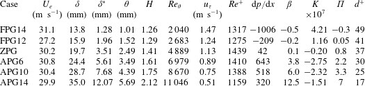
Summary of parameters for the simulated cases at Mach 0.5 with pressure gradients:
 $U_{e}$
and
 $u_{\unicode[STIX]{x1D70F}}$
are the free stream and friction velocities at the middle of the domain of interest. The two values for
 $\unicode[STIX]{x0394}y^{+}$
indicate the mesh spacing at the wall (subscript
 $w$
) and at the boundary-layer edge (subscript
 $e$
).
 $\unicode[STIX]{x1D6FC}$
is the angle of the slanted wall used to impose a prescribed pressure gradient.

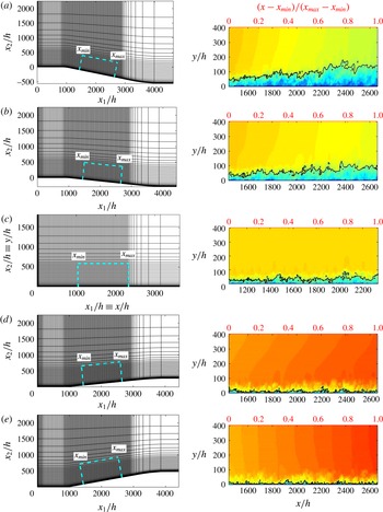
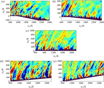
Two-dimensional slices of the computational grids in the left column. Every ten points are shown and the thick dashed lines define the domain of interest in the
 $(x_{1},x_{2})$
-plane. The reference length is the height
 $h$
of the backward-facing step located upstream of the domain and involved in the turbulence triggering method. Instantaneous views of the streamwise velocity field
 $u$
in the domain of interest after rotation in the right column for the different configurations: APGs (a), APGw (b), ZPG (c), FPGw (d) and FPGs (e). The black isocontour corresponds to
 $u=140~\text{m}~\text{s}^{-1}$
and highlights the boundary-layer thickening (with a scale factor of 3 in the vertical direction).

2.2 Grid design and flow parameters
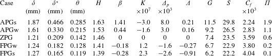
The data analysed in the paper are obtained from a series of simulations, whose main parameters are summarized in table 1. Five values of the pressure gradient are considered by keeping a horizontal free stream and changing the angle
 $\unicode[STIX]{x1D6FC}$
of the plate. The Mach number based on the free stream velocity is fixed at
 $M=U_{\infty }/c_{\infty }=0.5$
. The free stream thermodynamic quantities are
 $p_{\infty }=101\,300~\text{Pa}$
and
 $T_{\infty }=298.15~\text{K}$
.
Side views of the grids are presented in the left column of figure 2. The ZPG mesh is the same as that of the simulations of Gloerfelt & Margnat (Reference Gloerfelt and Margnat2014) and is discretized with
 $1440\times 400\times 400$
points. Grid points are equally spaced in the spanwise direction and are clustered near the wall using a geometric progression of 2 % for the first 25 points, then with a rate of 2.5 % for the following 155 points. The distribution is then uniform for the next 120 points and a stretching is finally applied to the last 100 points up to the top boundary (visible in figure 2
c for
 $y_{2}/h\gtrsim 600$
). In the streamwise direction, the grid points are clustered near the inlet over a range of 200 points, so that small grid sizes are used for properly entering unstable modes. The grid spacing is then regular up to the exit zone where a grid stretching with a geometric progression of 3 % is applied over the last 100 points to create a large sponge zone where the flow variables are progressively filtered with a Laplacian operator at each time step to minimize numerical reflections from the outlet.
For the non-zero-pressure-gradient cases, a curvilinear domain of
 $1600\times 400$
points is defined and extruded in the third direction on
 $n_{z}=400$
points. Along the
 $x_{1}$
-direction parallel to the external free stream, a first region of horizontal plate is defined in order to have the same inlet condition as the ZPG case. Note that the grid spacing is also refined on the first 150 points near the inlet boundary and is maintained constant for the next 200 points with a spacing slightly greater than the one in the zone of interest above the ramp. This second region corresponds to an inclined plate with an angle
 $\unicode[STIX]{x1D6FC}$
from the horizontal, which is negative for the adverse-pressure-gradient cases and positive for the favourable-pressure-gradient cases. The values of
 $\unicode[STIX]{x1D6FC}$
are reported in table 1 and are chosen to set the strength of the pressure gradient. The points are equally spaced on the ramp region with the nominal streamwise spacing. The third part of the mesh represents the exit zone where a horizontal plate is recovered with a severe stretching on the last 100 points. Note that the two transitions between the ramp and the flat portions are progressive and corresponds to a low radius of curvature set on approximately 30 grid points. The distribution of points in the wall-normal direction is the same as the ZPG case and the mesh is also regular in the spanwise direction.
The wall-pressure analyses are restricted to a zone of interest where a nearly equilibrium TBL flow is obtained. This area is defined between curvilinear abscissae
 $x_{min}$
and
 $x_{max}$
and is delimited by thick dashed lines in the left column of figure 2. These zones of interest for each cases exclude the transitional development zone, the exit sponge zone and the upper buffer region. For the non-zero-pressure-gradient cases, the domain of interest in the
 $(x_{1},x_{2})$
-plane where the plate is inclined is transformed into a Cartesian
 $(x,y)$
-plane where the plate is horizontal using a rotation and an interpolation of the variables. In the subsequent flow analyses,
 $u=\cos (\unicode[STIX]{x1D6FC})u_{1}+\sin (\unicode[STIX]{x1D6FC})u_{2}$
and
 $v=-\sin (\unicode[STIX]{x1D6FC})u_{1}+\cos (\unicode[STIX]{x1D6FC})u_{2}$
are the
 $x$
-component parallel to the wall and
 $y$
-component normal to the wall of the velocity respectively, where
 $u_{1},u_{2}$
are the components defined in the
 $(x_{1},x_{2})$
-plane and used in the governing equations (2.1). From now on, the coordinate system
 $(x,y,z)$
is used and the velocity components are denoted
 $(u,v,w)$
. The right column of figure 2 shows the streamwise component
 $u$
on the rotated domain restricted to the interest zone between
 $x_{min}$
and
 $x_{max}$
. It is noteworthy that the grid spacing in this region is regular in the
 $x$
- and
 $z$
-directions, and that the physical values of the spacings
 $\unicode[STIX]{x0394}x$
,
 $\unicode[STIX]{x0394}z$
and
 $\unicode[STIX]{x0394}y_{min}$
are the same for all simulations. They are given in table 1 in terms of wall units evaluated at the middle of the domain of interest (based on the friction velocity
 $u_{\unicode[STIX]{x1D70F}}$
and the viscous length scale
 $\ell _{v}=\unicode[STIX]{x1D708}/u_{\unicode[STIX]{x1D70F}}$
). The subscript
 $w$
is used to denote quantities evaluated at the wall and the subscript
 $e$
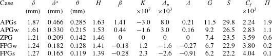
quantities evaluated at the edge of the boundary layer. In the tables 1 and 2, the quantities representative of the different configurations are taken at the middle of the domain of interest
 $(x_{max}-x_{min})/2$
, which are very close to the values averaged over
 $[x_{min},x_{max}]$
. The streamwise length of the domain of interest in terms of outer variables is
 $104.8\unicode[STIX]{x1D6FF}^{\ast }$
for APGs,
 $148.0\unicode[STIX]{x1D6FF}^{\ast }$
for APGw,
 $246.3\unicode[STIX]{x1D6FF}^{\ast }$
for ZPG,
 $268.3\unicode[STIX]{x1D6FF}^{\ast }$
for FPGw and
 $295.9\unicode[STIX]{x1D6FF}^{\ast }$
for FPGs.
Boundary layer properties and parameters quantifying the pressure gradient at the middle of the domain of interest.
The time step for all simulations is
 $\unicode[STIX]{x0394}t=\text{CFL}\unicode[STIX]{x0394}y_{min}/(U_{\infty }+c_{\infty })\simeq 0.025h/U_{\infty }$
, corresponding to a Courant–Friedrichs–Lewy number
 $\text{CFL}=1.5$
. The total simulation time is roughly the same for the different cases,
 $t=20\,000h/U_{\infty }$
. Statistical quantities are averaged over time and the spanwise direction. Wall-pressure planes are stored every
 $30\unicode[STIX]{x0394}t$
during the last
 $240\,000$
iterations, corresponding to 8000 samples and a non-dimensional time of approximately
 $6000h/U_{\infty }$
or
 $4.9(x_{max}-x_{min})/U_{\infty }$
.
3 Flow results
3.1 Pressure-gradient parameters
Figure 2 shows instantaneous views of the simulated TBLs over the domain of interest. The principal characteristics of the different simulations are summarized in tables 1 and 2. The pressure gradient in boundary-layer flows can be characterized by a variety of non-dimensional parameters, some of them are listed in table 2. The Clauser pressure-gradient parameter
 $\unicode[STIX]{x1D6FD}$
, the acceleration parameter
 $K$
(Kline et al.
Reference Kline, Reynolds, Schraub and Runstadler1967), the viscous-scaled pressure gradient
 $\unicode[STIX]{x1D6E5}_{p}$
and the Castillo & George (Reference Castillo and George2001) pressure-gradient parameter
 $\unicode[STIX]{x1D6EC}$
are defined as
 $$\begin{eqnarray}\unicode[STIX]{x1D6FD}=\frac{\unicode[STIX]{x1D6FF}^{\ast }}{\unicode[STIX]{x1D70F}_{w}}\frac{\text{d}P_{e}}{\text{d}x},\quad K=\frac{\unicode[STIX]{x1D708}}{U_{e}^{2}}\frac{\text{d}U_{e}}{\text{d}x},\quad \unicode[STIX]{x1D6E5}_{p}=\frac{\unicode[STIX]{x1D708}}{\unicode[STIX]{x1D70C}u_{\unicode[STIX]{x1D70F}}^{3}}\frac{\text{d}P_{e}}{\text{d}x},\quad \unicode[STIX]{x1D6EC}=\frac{\unicode[STIX]{x1D6FF}}{\unicode[STIX]{x1D70C}U_{e}^{2}(\text{d}\unicode[STIX]{x1D6FF}/\text{d}x)}\frac{\text{d}P_{e}}{\text{d}x},\quad\end{eqnarray}$$
where
 $U_{e}$
and
 $P_{e}$
are the mean streamwise velocity and local static pressure, respectively, at the edge of the boundary layer. In the following,
 $\unicode[STIX]{x1D6FF}$
,
 $\unicode[STIX]{x1D6FF}^{\ast }$
,
 $\unicode[STIX]{x1D703}$
denote the 99 %-, displacement and momentum thicknesses,
 $\unicode[STIX]{x1D70F}_{w}$
is the wall stress,
 $u_{\unicode[STIX]{x1D70F}}$
the friction velocity and
 $\unicode[STIX]{x1D708}$
is the kinematic viscosity. The TBL is also characterized by its shape factor
 $H$
and the defect shape factor
 $G$
defined as
 $$\begin{eqnarray}H=\frac{\unicode[STIX]{x1D6FF}^{\ast }}{\unicode[STIX]{x1D703}},\quad S=\frac{U_{e}}{u_{\unicode[STIX]{x1D70F}}}=\sqrt{\frac{2}{C_{f}}},\quad G=S\left(1-\frac{1}{H}\right).\end{eqnarray}$$
The defect law (Clauser Reference Clauser1954; Coles Reference Coles1956),
 $(U_{e}-\overline{u})/u_{\unicode[STIX]{x1D70F}}$
, for the mean streamwise velocity
 $\overline{u}$
can be used to define the wake parameter
 $\unicode[STIX]{x1D6F1}$
, which is also a measure of the free stream pressure gradient. The values obtained for the pressure-gradient parameters correspond to mild intensities, which can be encountered for instance over the cockpit of an airplane.
In the following, the mean and fluctuating aerodynamic quantities are analysed and validated with respect to the published literature. Beforehand it has been carefully checked that different criteria for self-similarity and equilibrium are fulfilled.
3.2 Notion of equilibrium
First we check the equilibrium character for the boundary layers subjected to a pressure gradient. The reason is twofold. First, the analysis of the wall pressure in the frequency–wavenumber space requires an assumption of homogeneity in the streamwise direction. This is the case in a fully turbulent channel flow (Viazzo, Dejoan & Schiestel Reference Viazzo, Dejoan and Schiestel2001; Hu, Morfey & Sandham Reference Hu, Morfey and Sandham2002, Reference Hu, Morfey and Sandham2006) but is only an approximation for a developing turbulent boundary layer due to its thickening. Equilibrium flows exhibit a self-similarity of mean and turbulent velocity profiles, so that the flow dynamics is similar over the domain of interest, and we follow the classical assumption that the slow thickening along
 $x$
can be neglected. Second, it is well known that the flow responds differently if the force of the pressure gradient is constant or varying in space or in time. The boundary layers subjected to an adverse gradient are especially very dependent on the upstream history and the way the gradient is applied. This is clearly a difficulty when comparing different databases. We hope this limitation can be circumvented by using equilibrium TBLs.
There is not a unique definition of equilibrium. It can be defined as the fact of obtaining a balance, that is to say the same relative weight between different terms of the governing equations. Some equilibrium can be reached without self-similar profiles. In fact a rigorous equilibrium is never reached for turbulent boundary layers since they depend on two scales (inner and outer). The only exception is sink flow, where the strength of the favourable pressure gradient leads to converging mean streamlines, and the law of the wake vanishes so that only an inner law can describe the mean quantities. We talk about ‘traditional’ equilibrium if a self-similarity is seen to exist for the mean streamwise velocity and for the Reynolds stress components. The boundary-layer thickness
 $\unicode[STIX]{x1D6FF}$
is often used as the length scale. Traditionally, the friction velocity
 $u_{\unicode[STIX]{x1D70F}}$
is chosen as the velocity scale: see e.g. Coles (Reference Coles1956) who successfully collapsed defect laws for different classes of flows. Castillo & George (Reference Castillo and George2001) suggested the use of
 $U_{e}$
, but this is not a turbulent velocity scale. They also introduced the use of the velocity scaling proposed by Zaragola & Smits (Reference Zaragola and Smits1997), namely
 $U_{ZS}=U_{e}\unicode[STIX]{x1D6FF}^{\ast }/\unicode[STIX]{x1D6FF}$
which seems to be the best velocity scale to extend the traditional equilibrium following Maciel, Rossignol & Lemay (Reference Maciel, Rossignol and Lemay2006). The latter have tested the different scalings for strong APG or nearly separated flows, and concluded that
 $U_{ZS}$
provides an acceptable self-similarity for both the defect law and the Reynolds stresses. Once again a rigorous equilibrium is difficult to achieve and is rather the exception than the rule. There are more papers describing the equilibrium conditions than experimental realizations which achieved a ‘good’ equilibrium. The reader is referred to discussions of Clauser (Reference Clauser1954), Coles (Reference Coles1956), Townsend (Reference Townsend1961), Rotta (Reference Rotta1962), Mellor (Reference Mellor1966), Kader & Yaglom (Reference Kader and Yaglom1981), Schofield (Reference Schofield1981), Tani (Reference Tani1986), Castillo & George (Reference Castillo and George2001), Maciel et al. (Reference Maciel, Rossignol and Lemay2006). We can summarize the traditional equilibrium conditions as follows:
-
(i) a power-law relation between
 $U_{e}$
and
$x$
is necessary, i.e.
$U_{e}\sim L_{0}^{-\unicode[STIX]{x1D6EC}}\sim (x-x_{0})^{-\unicode[STIX]{x1D6EC}}$
(Townsend Reference Townsend1961);
-
(ii) as a consequence the outer length scale will vary linearly with
$x$
, i.e.
$L_{0}\sim (x-x_{0})$
; -
(iii) some of the gradient parameters
$\unicode[STIX]{x1D6FD}$
,
$K$
,
$\unicode[STIX]{x1D6E5}_{p}$
,
$\unicode[STIX]{x1D6EC}$
defined by (3.1) or defect-law parameters
$G$
or
$\unicode[STIX]{x1D6F1}$
defined by (3.2) should remain constant along
$x$
.





The two last conditions (ii) and (iii) also imply that the outer length scale
 $\unicode[STIX]{x1D6FF}$
grows linearly, the ratios
 $\unicode[STIX]{x1D6FF}/\unicode[STIX]{x1D6FF}^{\ast }$
and
 $\unicode[STIX]{x1D6FF}/\unicode[STIX]{x1D703}$
are constant, thus
 $\unicode[STIX]{x1D6FF}^{\ast }$
and
 $\unicode[STIX]{x1D703}$
also evolve as
 $x-x_{0}$
.
Free stream velocity
 $U_{e}$
evolution: (a) log–log plot of
 $U_{e}$
versus
 $\unicode[STIX]{x1D6FF}$
for APGs (


 $\unicode[STIX]{x1D6EC}=0.24$
(APGs); 0.18 (APGw); 0 (ZPG);
 $-$
0.28 (FPGw);
 $-$
0.92 (FPGs). (b)
 $U_{e}$
versus
 $x$
in non-dimensionalized form. Solid lines represent
 $(x-x_{0})^{-\unicode[STIX]{x1D6EC}}$
curves.

To determine if there exists a power-law relation between
 $U_{e}$
and
 $\unicode[STIX]{x1D6FF}$
, we plot
 $U_{e}$
versus
 $\unicode[STIX]{x1D6FF}$
in a log–log plot (Castillo & George Reference Castillo and George2001; Maciel et al.
Reference Maciel, Rossignol and Lemay2006) in figure 3(a). A linear regression provides the values of the exponent from 0.24 for adverse to
 $-$
0.92 for favourable case. As a comparison, Skare and Krogstad obtained
 $\unicode[STIX]{x1D6EC}=0.22$
and Maciel et al. (Reference Maciel, Rossignol and Lemay2006) report values of 0.22 and 0.3 in experiments of Samuel & Joubert (Reference Samuel and Joubert1974) and Marusic & Perry (Reference Marusic and Perry1995) for non-equilibrium APG flows. Values between 0.16 and 0.2 are reported for nearly separated TBLs. Figure 3(b) shows fair comparisons of
 $U_{e}$
with
 $(x-x_{0})^{-\unicode[STIX]{x1D6EC}}$
by using the previously obtained exponent and extrapolating the virtual origin
 $x_{0}$
.
Development of boundary-layer thickness,
 $\unicode[STIX]{x1D6FF}$
(

 $\unicode[STIX]{x1D6FF}^{\ast }$
(

 $\unicode[STIX]{x1D703}$
(

 $\unicode[STIX]{x1D6FF},\unicode[STIX]{x1D6FF}^{\ast },\unicode[STIX]{x1D703}$
for APGs (equilibrium over
 $28\unicode[STIX]{x1D6FF}_{av}$
); (b)
 $\unicode[STIX]{x1D6FF},\unicode[STIX]{x1D6FF}^{\ast },\unicode[STIX]{x1D703}$
for APGw (equilibrium over
 $30\unicode[STIX]{x1D6FF}_{av}$
); (c)
 $\unicode[STIX]{x1D6FF},\unicode[STIX]{x1D6FF}^{\ast },\unicode[STIX]{x1D703}$
for ZPG (equilibrium over
 $40\unicode[STIX]{x1D6FF}_{av}$
); (d)
 $\unicode[STIX]{x1D6FF},\unicode[STIX]{x1D6FF}^{\ast },\unicode[STIX]{x1D703}$
for FPGw (equilibrium over
 $40\unicode[STIX]{x1D6FF}_{av}$
); (e)
 $\unicode[STIX]{x1D6FF},\unicode[STIX]{x1D6FF}^{\ast },\unicode[STIX]{x1D703}$
for FPGs (equilibrium over
 $38\unicode[STIX]{x1D6FF}_{av}$
).

The linear growth of the three boundary-layer thicknesses with streamwise distance is checked in figure 4. The thicknesses are normalized by their averaged value over [
 $x_{min}$
,
 $x_{max}$
]. A linear evolution is visible over a length of 30 to
 $40\unicode[STIX]{x1D6FF}_{av}$
. In the figures, linear fits of the data in the self-similar region are extended toward 0 to check if the virtual origin
 $x_{0}$
is reached. This is confirmed for the APGs flow but less good for the other flows.
 $\unicode[STIX]{x1D6FF}^{\ast }$
and
 $\unicode[STIX]{x1D703}$
have the same origin, but the slope for
 $\unicode[STIX]{x1D6FF}$
is slightly smaller. It is most noticeable for the FPGs case since the virtual origin is around
 $150\unicode[STIX]{x1D6FF}_{av}$
ahead of
 $x_{min}$
. We can indeed see in figure 5(a,b) that the ratios
 $\unicode[STIX]{x1D6FF}/\unicode[STIX]{x1D6FF}^{\ast }$
and
 $\unicode[STIX]{x1D6FF}/\unicode[STIX]{x1D703}$
are only approximately constant (a slight decrease is observed). The shape factor, plotted in figure 5(c), is also relatively constant over the interest zone, with increasing values from favourable to adverse gradients. Some authors (Hu & Herr Reference Hu and Herr2016) propose to use these values for characterizing the gradient intensity.
Ratios of boundary-layer thicknesses,
 $\unicode[STIX]{x1D6FF}/\unicode[STIX]{x1D6FF}^{\ast }$
(a),
 $\unicode[STIX]{x1D6FF}/\unicode[STIX]{x1D703}$
(b) and shape factor
 $H=\unicode[STIX]{x1D6FF}^{\ast }/\unicode[STIX]{x1D703}$
(c). APGs (


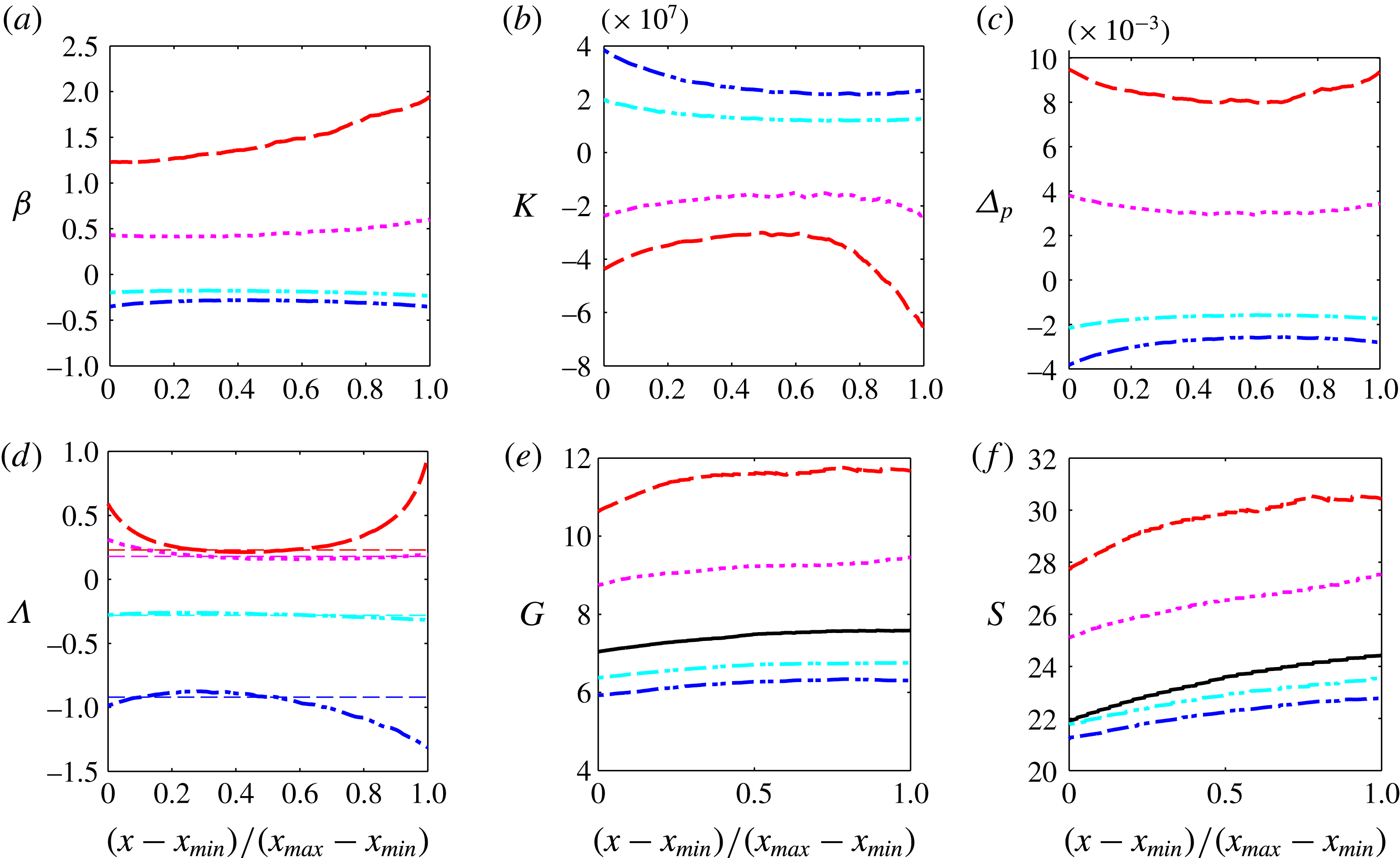
The streamwise evolution of the gradient parameters is depicted in figure 6. Considering the range in ordinate axis, the constant character is more or less observed. Discrepancies can be noted for the APGs flow, notably at the end of the interest zone. But the variation of
 $\unicode[STIX]{x1D6FD}$
from 1.23 to 1.94 can be considered as relatively weak when compared to those encountered in experiments with adverse gradients (Kline et al.
Reference Kline, Reynolds, Schraub and Runstadler1967; Skare & Krogstad Reference Skare and Krogstad1994; Nagano, Tsuji & Houra Reference Nagano, Tsuji and Houra1998). For the FPGs case, the flow is not fully established at the beginning of the interest region, as illustrated by the acceleration parameter
 $K$
. The Castillo & George (Reference Castillo and George2001) parameter
 $\unicode[STIX]{x1D6EC}$
also exhibits non-constant values at the beginning and at the end of the selected region for the strong gradient cases. This parameter should be equivalent to the exponent evaluated directly in figure 3 (Castillo & George Reference Castillo and George2001). The values determined in figure 3, corresponding to the horizontal dashed lines in figure 6(d), are indeed in very good agreement with those from the definition (3.1), at least in the centre of the domain of interest for the strongest gradient cases. The exponent for the two adverse-gradient flows are close (
 $\unicode[STIX]{x1D6EC}=0.24$
for APGs and 0.18 for APGw). Castillo & George (Reference Castillo and George2001) found values ranging from 0.18 to 0.28 by fitting different experimental data sets. They claim that APG boundary layers might be characterized by a single value,
 $\unicode[STIX]{x1D6EC}\approx 0.22$
. We feel that the value depends on the gradient intensity. By analysing two favourable-gradient TBLs, Castillo & George (Reference Castillo and George2001) conclude that FPG boundary layers are also characterized by a single value of
 $\unicode[STIX]{x1D6EC}$
(
 $\unicode[STIX]{x1D6EC}\approx -1.92$
). In the present numerical experiment, we have found different values, namely
 $-$
0.28 for FPGw and
 $-$
0.92 for FPGs, invalidating their assumption. The value of
 $\unicode[STIX]{x1D6EC}$
appears more dependent on the pressure-gradient force for FPG flows.
Overall, compared to previous experimental databases, the range of variations of the different pressure-gradient parameters along the interest domain is sufficiently small to consider that we have reached equilibrium flows.
Streamwise evolution of the Clauser pressure gradient parameter
 $\unicode[STIX]{x1D6FD}$
(a), acceleration parameter
 $K$
(b), viscous-scaled pressure gradient
 $\unicode[STIX]{x1D6E5}_{p}$
(c), Castillo & George (Reference Castillo and George2001) parameter
 $\unicode[STIX]{x1D6EC}$
(d), defect shape factor
 $G$
(e) and ratio
 $S$
(f). The horizontal dashed lines in (d) correspond to exponent values determined in figure 3(a).

3.3 Velocity profiles and similarity scales
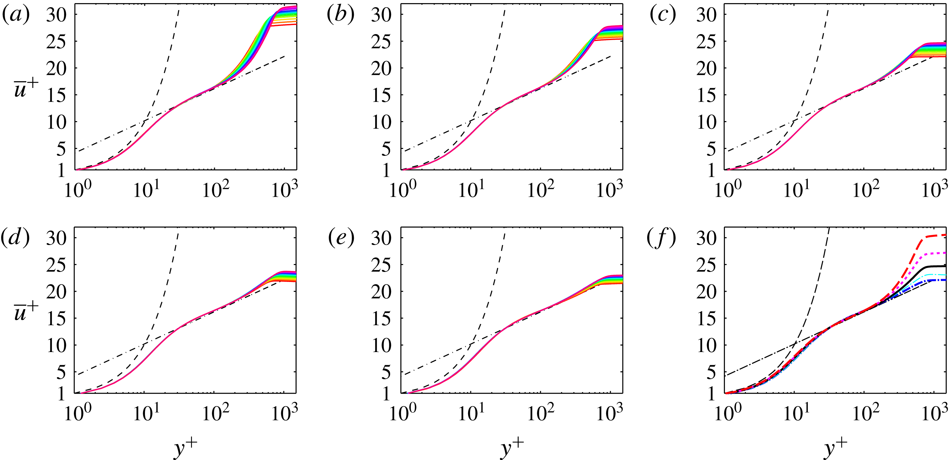
Figure 7 shows the mean streamwise velocity profiles scaled with inner variables (
 $\overline{u}^{+}=\overline{u}/u_{\unicode[STIX]{x1D70F}}$
and
 $y^{+}=yu_{\unicode[STIX]{x1D70F}}/\unicode[STIX]{x1D708}$
) for all the five pressure-gradient flows. Two notable features can be observed. First, all the profiles collapse in the inner region (
 $y\leqslant 0.1\unicode[STIX]{x1D6FF}$
). This was expected due to the mild magnitude of the pressure gradients imposed, as also observed for instance by Harun et al. (Reference Harun, Monty, Mathis and Marusic2013) with moderate pressure gradients. A deviation of the mean velocity profile from the classical log law has been reported for stronger pressure gradients (Skare & Krogstad Reference Skare and Krogstad1994; Nagano et al.
Reference Nagano, Tsuji and Houra1998; Nagib & Chauhan Reference Nagib and Chauhan2008; Monty, Harun & Marusic Reference Monty, Harun and Marusic2011). This effect is visible for instance in the profiles of Nagano et al. (Reference Nagano, Tsuji and Houra1998) plotted in figure 11(a). Note that this feature can only be investigated if a direct evaluation of the friction velocity
 $u_{\unicode[STIX]{x1D70F}}$
is performed (Nagib & Chauhan Reference Nagib and Chauhan2008). Since the present simulations use large-eddy simulation resolutions, a direct evaluation of
 $u_{\unicode[STIX]{x1D70F}}$
from
 $\unicode[STIX]{x2202}\overline{u}/\unicode[STIX]{x2202}y$
at the wall leads to an underestimation of the friction velocity. To allow comparisons, we have therefore computed
 $u_{\unicode[STIX]{x1D70F}}$
by fitting the profiles with analytical inner profiles. We used the law of Musker (Reference Musker1979), who proposed a simple formula valid from the viscous sublayer (
 $y^{+}<5$
, where
 $U^{+}=y^{+}$
) up to the overlap region where the log law is assumed. The formulation of Chauhan, Monkewitz & Nagib (Reference Chauhan, Monkewitz and Nagib2009) is used:
 $$\begin{eqnarray}\displaystyle U_{inner}^{+} & = & \displaystyle \frac{1}{\unicode[STIX]{x1D705}}\ln \left(\frac{y^{+}-a}{-a}\right)+\frac{R^{2}}{a(4\unicode[STIX]{x1D6FC}-a)}\left[(4\unicode[STIX]{x1D6FC}+a)\ln \left(-\frac{a}{R}\frac{\sqrt{(y^{+}-\unicode[STIX]{x1D6FC})^{2}+B^{2}}}{y^{+}-a}\right)\right.\nonumber\\ \displaystyle & & \displaystyle +\left.\frac{\unicode[STIX]{x1D6FC}}{B}(4\unicode[STIX]{x1D6FC}+5a)\left(\arctan \left(\frac{y^{+}-\unicode[STIX]{x1D6FC}}{B}\right)+\arctan \left(\frac{\unicode[STIX]{x1D6FC}}{B}\right)\right)\right],\end{eqnarray}$$
where
 $\unicode[STIX]{x1D6FC}=(-1/\unicode[STIX]{x1D705}-a)/2$
,
 $B=\sqrt{-2a\unicode[STIX]{x1D6FC}-\unicode[STIX]{x1D6FC}^{2}}$
and
 $R=\sqrt{\unicode[STIX]{x1D6FC}^{2}+B^{2}}$
. The value for the parameter
 $a$
is set at
 $-$
10.5531 so that the constants of the log law are (
 $\unicode[STIX]{x1D705}=0.41$
,
 $B=5$
). Even if the logarithmic region is difficult to assess for low Reynolds number turbulent boundary layers, some authors found that the log law having constants
 $\unicode[STIX]{x1D705}=0.41$
and
 $B=5$
is a good approximation for fitting velocity profiles at low Reynolds numbers (see Erm & Joubert (Reference Erm and Joubert1991) and references therein). Note that using these constants for all cases, we are not able to evaluate deviations from the classical log law due to the presence of the pressure gradients.
Mean velocity profiles in wall units
 $\overline{u}^{+}$
: thirteen profiles between
 $x_{min}$
and
 $x_{max}$
for APGs (a), APGw (b), ZPG (c), FPGw (d) and FPGs (e). Comparison of the five cases at similar friction Reynolds number
 $Re_{\unicode[STIX]{x1D70F}}\simeq 748$
(f).

The second noticeable feature, seen in figure 7(f), is the consistent increase of the mean velocity relative to
 $u_{\unicode[STIX]{x1D70F}}$
in the wake region with pressure gradient, which is a classical feature and is better analysed by considering the defect law, as shown by Clauser (Reference Clauser1954) or Coles (Reference Coles1956). Following these authors, the mean velocity profiles can be decomposed as the sum of an inner law and a wake law:
 $$\begin{eqnarray}U_{composite}^{+}=U_{inner}^{+}+\frac{\unicode[STIX]{x1D6F1}}{\unicode[STIX]{x1D705}}{\mathcal{W}}\left(\frac{y}{\unicode[STIX]{x1D6FF}}\right).\end{eqnarray}$$
The universal form suggested by Coles (Reference Coles1956) being incapable of satisfying the condition
 $\text{d}U^{+}/\text{d}y=0$
at the edge of the boundary layer, the wake law of Lewkowicz (Reference Lewkowicz1982) is retained in the present work:
 $$\begin{eqnarray}{\mathcal{W}}\left(\frac{y}{\unicode[STIX]{x1D6FF}}\right)=2\left(\frac{y}{\unicode[STIX]{x1D6FF}}\right)^{2}\left(3-2\frac{y}{\unicode[STIX]{x1D6FF}}\right)-\frac{1}{\unicode[STIX]{x1D6F1}}\left(\frac{y}{\unicode[STIX]{x1D6FF}}\right)^{2}\left(1-\frac{y}{\unicode[STIX]{x1D6FF}}\right)\left(1-2\frac{y}{\unicode[STIX]{x1D6FF}}\right).\end{eqnarray}$$
The composite profiles are depicted in figure 8 with outer scaling by
 $\unicode[STIX]{x1D6FF}$
and
 $U_{e}$
. Here Musker’s law (3.3) is used for
 $U_{inner}^{+}$
. The wake parameter
 $\unicode[STIX]{x1D6F1}$
is given for each case in the last column of table 2 and evaluated by matching computed defect law with expression obtained using (3.5) (see figure 9
a). For all pressure-gradient cases, a very good similarity is obtained for the thirteen successive profiles over the region of interest.
Comparison of mean velocity profiles with composite expression (3.4) (

 $=$
wake law
 $\unicode[STIX]{x1D6F1}{\mathcal{W}}/\unicode[STIX]{x1D705}$
(

 $+$
inner law
 $U_{inner}^{+}$
(

 $x_{min}$
and
 $x_{max}$
for APGs


The mean streamwise velocity profiles are represented as defect laws in figure 9. The two favourable cases are close so that the FPGw curves are omitted for clarity. The classical defect law, where the velocity scale is the friction velocity
 $u_{\unicode[STIX]{x1D70F}}$
(Coles Reference Coles1956), is plotted in 9(a) for thirteen successive locations along the plate. The symbols correspond to the theoretical law (3.5) by adjusting the wake parameter
 $\unicode[STIX]{x1D6F1}$
(reported in the last column of table 2). The increase of
 $\unicode[STIX]{x1D6F1}$
from FPG to APG conforms to the trends in the literature, even if we noticed slightly higher values associated with compressibility effects (Gloerfelt & Margnat Reference Gloerfelt and Margnat2014). It is worth noting that the self-similarity of the defect law is perfectible, notably for the APGs case. That is why we tried other scalings. A slight improvement is visible by using the free stream velocity
 $U_{e}$
as proposed by Castillo & George (Reference Castillo and George2001) but a better collapse is observed with the Zaragola & Smits (Reference Zaragola and Smits1997) velocity
 $U_{ZS}=U_{e}\unicode[STIX]{x1D6FF}^{\ast }/\unicode[STIX]{x1D6FF}$
, as suggested by Maciel et al. (Reference Maciel, Rossignol and Lemay2006). Furthermore, the curves for the different gradients collapse remarkably to a single curve.
Self-similarity of the defect law with
 $u_{\unicode[STIX]{x1D70F}}$
-scaling (a),
 $U_{e}$
-scaling (b) and
 $U_{ZS}$
-scaling (c) (APGs


 $\unicode[STIX]{x1D6F1}$
.

Similarity of Reynolds shear stresses with
 $U_{e}$
-scaling (a),
 $u_{\unicode[STIX]{x1D70F}}$
-scaling (b),
 $U_{ZS}$
-scaling (c) as a function of the outer coordinate
 $y/\unicode[STIX]{x1D6FF}$
and inner scaling
 $u_{rms}^{+}$
versus
 $y^{+}$
(d). Twelve profiles between
 $x_{min}$
and
 $x_{max}$
for APGs (


Another necessary condition for equilibrium is the self-similarity of Reynolds shear stress profiles and is tested in figure 10. By plotting profiles for successive streamwise locations, the Reynolds number dependency is clearly visible using wall coordinates (figure 10
d). The use of
 $u_{\unicode[STIX]{x1D70F}}$
or
 $U_{e}$
as velocity scales in figure 10(a,b) shows a degree of self-similarity for FPG or ZPG flows, which is however less apparent for APG flows. The scaling with
 $U_{ZS}$
in figure 10(c) provides a better collapse, confirming the improvements already observed with this velocity scale for the defect law. The Zaragola–Smits velocity is thus an appropriate outer scale for both velocity and turbulent intensities. Wosnik & George (Reference Wosnik and George2000) and Castillo & Wang (Reference Castillo and Wang2004) interpret the success of the Zaragola–Smits scaling by considering that the ratio
 $\unicode[STIX]{x1D6FF}^{\ast }/\unicode[STIX]{x1D6FF}$
, appearing in
 $U_{ZS}$
, includes a kind of Reynolds number dependence and upstream history of the TBL.
Comparison of mean velocity profiles in wall units with experiments for adverse (a) and favourable (b) gradients. Present LES: APGs (


 $\unicode[STIX]{x1D6FD}=0$

 $\unicode[STIX]{x1D6FD}=0.7$

 $\unicode[STIX]{x1D6FD}=2.19$

 $\unicode[STIX]{x1D6FD}=3.95$

 $\unicode[STIX]{x1D6FD}=5.32$

 $\unicode[STIX]{x1D6FD}=-0.35$
,
 $x=2$
and 3 ft

 $K=2.7\times 10^{7}$
,
 $x=0.8~\text{m}$

 $x=2.2~\text{m}$


3.4 Comparisons with experiments
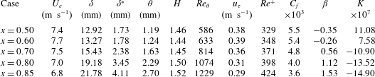
Let us compare the mean velocity profiles with some experimental databases in figures 11 and 12. For the APG boundary layers, we selected the low Reynolds number experiments of Nagano et al. (Reference Nagano, Tsuji and Houra1998), who studied the development of a non-equilibrium adverse pressure gradient TBL. The Clauser parameter
 $\unicode[STIX]{x1D6FD}$
varies between 0 and 5.3, with
 $Re_{\unicode[STIX]{x1D703}}$
ranging between 1290 and 3350. The median value for the momentum thickness Reynolds number is roughly 2500 for APGw and 3000 for APGs. The comparison of the Reynolds stresses in figure 12(a–c) shows good compliance for the ZPG flows, with a slight underprediction in the simulation due to the LES resolution, notably for the spanwise root-mean-square (rms) velocity
 $w_{rms}$
. In figure 12(b), the APGw profile (
 $\unicode[STIX]{x1D6FD}\approx 0.5$
) matches the measurements for
 $\unicode[STIX]{x1D6FD}=0.77$
, and the APGs profile (
 $\unicode[STIX]{x1D6FD}\approx 1.6$
) is close to the profile at
 $\unicode[STIX]{x1D6FD}=2.19$
. The value of
 $\unicode[STIX]{x1D6FD}$
is not exactly the same since its evaluation is sensitive to flow history and the TBL of Nagano et al. (Reference Nagano, Tsuji and Houra1998) is not in equilibrium. The trends in our LES are thus in very good agreement with measurements. Visual inspection of the velocity profiles in figure 11(a) indicates that the measured profiles lie below the standard log-law profile as the adverse gradient is increased. Such an effect is not visible in the LES since, as explained previously, the friction velocity for wall scaling is deduced from Musker’s law which contains implicitly the standard logarithmic law. Furthermore, even for the ZPG TBL, the maximum mean velocity relative to
 $u_{\unicode[STIX]{x1D70F}}$
is greater in the simulations. We have indeed noticed an increase of the wake parameter from 0.6 to 0.9 by increasing the Mach number from 0.5 to 0.9 in a previous study on ZPG TBLs (Gloerfelt & Margnat Reference Gloerfelt and Margnat2014), whereas the commonly accepted value for incompressible ZPG TBL is 0.55. We can thus conclude that the comparison is further complicated by the compressibility effects at the moderate subsonic Mach number chosen in the simulations
 $(M=0.5)$
, whereas most of the measurements are done for low velocity incompressible flows.
Comparison of turbulent intensities
 $u_{rms}$
(a,d),
 $v_{rms}$
(b,e),
 $w_{rms}$
(c,f) with experiments for adverse (a–c) and favourable (d–f) gradients. Present LES: APGs (


 $\unicode[STIX]{x1D6FD}=0$

 $\unicode[STIX]{x1D6FD}=0.77$

 $\unicode[STIX]{x1D6FD}=2.19$

 $\unicode[STIX]{x1D6FD}=3.95$

 $\unicode[STIX]{x1D6FD}=5.32$

 $K=2.7\times 10^{7}$
,
 $x=0.8~\text{m}$

 $x=2.2~\text{m}$


The comparison is also fair for the mean profiles in wall units for FPG LES in figure 11(b) with the same tendency of a higher wake component in weakly compressible cases. We selected the mild-FPG boundary layer studied by Herring & Norbury (Reference Herring and Norbury1967) with
 $\unicode[STIX]{x1D6FD}=-0.35$
as for FPGs case, but with a higher Reynolds number (
 $Re_{\unicode[STIX]{x1D703}}\sim 5000{-}7000$
). The logarithmic region thus has a greater extent in the experiments of Herring & Norbury (Reference Herring and Norbury1967). We also compare with the well-documented sink-flow measurements of Jones et al. (Reference Jones, Marusic and Perry2001) with similar
 $Re_{\unicode[STIX]{x1D703}}$
(ranging between 1700 and 3000) and an acceleration parameter
 $K=2.7\times 10^{7}$
, close to that of the FPGs case (
 $K=2.3\times 10^{7}$
). The almost vanishing wake component is in good agreement between simulation and experiment. Moreover figure 12(d–f) shows that the decrease of the turbulent intensities in experiments is in fair agreement with FPGs boundary layer. Vertical and spanwise components are not correctly measured close to the wall. Further comparisons are provided in appendix A for experimental databases that also provide wall-pressure spectra. In particular, figure 23(a–d) shows very good compliance with the low Reynolds number direct numerical simulation (DNS) of Spalart & Watmuff (Reference Spalart and Watmuff1993). Recent measurement data of Hu & Herr (Reference Hu and Herr2016) and the simulation results are also in good agreement, as illustrated in figure 26(a–c).
4 Analysis of wall-pressure fluctuations
A thorough comparison with previous experimental and numerical databases is proposed to stress the main changes induced by the pressure gradient in a robust way. Recent studies that specifically deal with the influence of a pressure gradient on wall-pressure features are described in appendix A, where individual comparisons of mean flow profiles and autospectra are carried out. Elements about the method to obtain adverse or favourable gradients and the apparatus to measure wall pressure are given in appendix A to estimate the gradient intensity, the equilibrium character of the TBL or the resolution capabilities. These are necessary to draw firm conclusions. We concentrate on a number of specific questions related to the interpretation of power spectral densities and wavenumber–frequency spectra. In particular, since our computational strategy relies on direct noise calculations, we are able to provide the levels of the acoustic component for the first time.
4.1 Wall-pressure autospectra and global properties
The frequency power spectra of wall-pressure fluctuations
 $\unicode[STIX]{x1D719}(\unicode[STIX]{x1D714})$
are shown in figure 13. For each gradient case, the fluctuating pressure is stored on the wall mesh corresponding to the region of interest defined in § 2. The 8000 time samples, recorded every
 $30\unicode[STIX]{x0394}t$
, are divided into three segments with 50 % overlap, leading to a sampling frequency
 $f_{s}=1.33U_{\infty }/h$
. The inlet velocity
 $U_{\infty }$
and the step height
 $h$
are used for non-dimensionalization since they have the same physical values for all cases. With inner scaling, the sampling frequency is
 $\unicode[STIX]{x1D714}_{s}^{+}=2\unicode[STIX]{x03C0}\unicode[STIX]{x1D714}\unicode[STIX]{x1D708}/u_{\unicode[STIX]{x1D70F}}^{2}=10.3$
for ZPG case. Point spectra are evaluated at five streamwise locations along the region of interest, namely
 $x/h=\{1300,1500,1700,1900,2100\}$
for ZPG case and
 $x/h=\{1500,1700,1900,2100,2300\}$
for non-zero gradient cases (see figure 2), by averaging over the spanwise direction and over 100 points around the reference location in the streamwise direction. The spectra at the last location are presented in figure 13 as one-sided spectra. There is no universal scaling that collapses the pressure spectra of different Reynolds number flows at all frequencies. Three classical scalings are used in the present study, specifically outer scaling (local displacement thickness
 $\unicode[STIX]{x1D6FF}^{\ast }$
as the length scale, edge velocity
 $U_{e}$
as the velocity scale and dynamic pressure
 $q_{e}=0.5\unicode[STIX]{x1D70C}_{\infty }U_{e}^{2}$
as the pressure scale), mixed scaling (where the wall shear stress
 $\unicode[STIX]{x1D70F}_{w}$
replaces
 $q_{e}$
for the pressure scale) and inner scaling (local friction velocity
 $u_{\unicode[STIX]{x1D70F}}$
as the velocity scale, viscous length scale
 $\ell _{\unicode[STIX]{x1D708}}=\unicode[STIX]{x1D708}/u_{\unicode[STIX]{x1D70F}}$
and
 $\unicode[STIX]{x1D70F}_{w}$
as the pressure scale).
Frequency power spectra for the case APGs (


 $Re_{\unicode[STIX]{x1D703}}=1400$

 $Re_{\unicode[STIX]{x1D703}}=3321$
(ZPG25)

 $Re_{\unicode[STIX]{x1D703}}=6025$
(
 $U_{e}=28~\text{m}~\text{s}^{-1}$
)

 $Re_{\unicode[STIX]{x1D703}}=5527$
(APG25)

 $Re_{\unicode[STIX]{x1D703}}=11\,185$
(
 $7^{\circ }$
,
 $U_{\infty }=56~\text{ft}~\text{s}^{-1}$
)

 $Re_{\unicode[STIX]{x1D703}}=6979$
(APG6)

 $Re_{\unicode[STIX]{x1D703}}=12\,044$
(
 $12^{\circ }$
,
 $U_{\infty }=56~\text{ft}~\text{s}^{-1}$
)

 $Re_{\unicode[STIX]{x1D703}}=2683$
(FPG12)

 $Re_{\unicode[STIX]{x1D703}}=3932$
(
 $x=4.15$
)

 $R_{T}=20$
is plotted with a green dashed line, and the vertical dashed lines represent the estimated frequency cut-off of the LES for each case.

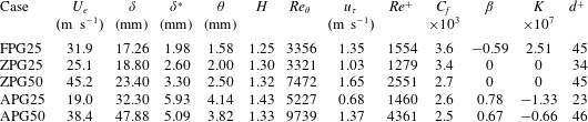
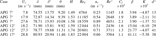
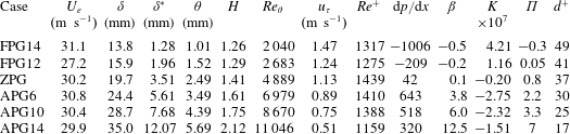
Figure 13 shows only outer and mixed scalings for the five investigated pressure gradients compared to selected measurements. Further comparisons with available results in the literature are compiled and commented in appendix A. Overall we found that the best scaling to collapse low and medium frequencies for TBLs subjected to different pressure gradients is the outer scaling. This is clear by inspection of comparisons with Na & Moin (Reference Na and Moin1998) in figure 23(e), Salze et al. (Reference Salze, Bailly, Marsden, Jondeau and Juvé2014) in figure 24(d) or Hu & Herr (Reference Hu and Herr2016) in figure 26(d). A maximum is reached around
 $\unicode[STIX]{x1D714}\unicode[STIX]{x1D6FF}^{\ast }/U_{e}\approx 0.4$
and the decay rate is smooth toward low frequencies. An approximate plateau is rather observed up to
 $\unicode[STIX]{x1D714}\unicode[STIX]{x1D6FF}^{\ast }/U_{e}\sim 1$
. With this scaling, its level is dependent on the Reynolds number, with slightly lower levels as
 $Re$
increases. The spectrum roll-off is highly dependent on the Reynolds number, with an enlargement of the intermediate-frequency range as the Reynolds number is increased. Even if the roll-off is precipitated by the spatial cut-off in the LES, this effect is visible since the local Reynolds number increases from FPGs to APGs due to the greater thickening of the TBL. Finally, the approximate collapse of a large part of the spectra is no longer valid for too strong APG or flows close to separation. The mixed scaling in figure 13(b) allows a clear distinction of the different gradients with increasing levels from favourable to adverse conditions. Some authors (Farabee & Casarella Reference Farabee and Casarella1991; Goody Reference Goody2004) have shown that the mixed scaling succeeds in attenuating the Reynolds number dependence in the medium-frequency range. The large amount of comparisons realized in the present study supports this proposal and indicates that it is also true for a given value of the pressure gradient. This representation also highlights the different decay rates in the intermediate-frequency range. The slopes are for instance plotted in figure 24(e) and increase from favourable to adverse conditions. In the present simulations, we found a power law
 $\unicode[STIX]{x1D714}^{-0.2}$
for FPGs,
 $\unicode[STIX]{x1D714}^{-0.5}$
for ZPG,
 $\unicode[STIX]{x1D714}^{-0.8}$
for APGw and
 $\unicode[STIX]{x1D714}^{-1.2}$
for APGs. Good compliance is obtained with the different spectra of Salze et al. (Reference Salze, Bailly, Marsden, Jondeau and Juvé2014) (not all displayed for brevity). It may also be noted that the exponent
 $-$
0.5 for ZPG is lower than the commonly accepted value of
 $-$
0.7, used in some models such as Goody (Reference Goody2004), and lower than the theoretical value
 $-$
1 (Panton & Linebarger Reference Panton and Linebarger1974). It appears that the value is influenced by the beginning of the spectral roll-off, and the slope increases with the Reynolds number. For instance, a value
 $-$
0.5 is found in ZPG LES (
 $Re^{+}\sim 700$
) and SONOBL experiments of Salze et al. (Reference Salze, Bailly, Marsden, Jondeau and Juvé2014) (
 $Re^{+}\sim 2500$
), a clear
 $\unicode[STIX]{x1D714}^{-0.7}$
-law is observed for high Reynolds numbers by Forest (Reference Forest2012) (
 $Re^{+}\sim 11\,100$
). At very high
 $Re$
for an atmospheric boundary layer (
 $Re^{+}\sim 10^{6}$
), Klewicki, Priyadarshana & Metzger (Reference Klewicki, Priyadarshana and Metzger2008) observed a
 $-$
1 slope.
Examples of inner scaling are presented in figures 23(f) and 24(f). The use of viscous scales allows a collapse of the spectra at high frequencies. This finding is still verified in the presence of a pressure gradient but the curve corresponds to higher frequencies from favourable to adverse conditions. The trend is also visible in the simulations even if the decay is rapid and sharp due to the grid cut-off in LES. It seems, however, that the commonly accepted viscous decay law
 $\unicode[STIX]{x1D714}^{-5}$
(Goody Reference Goody2004) would be weakly affected by pressure gradients.
Root-mean-square wall-pressure fluctuations normalized by viscous scaling
 $p_{rms}^{+}$
(a) or scaled on the dynamic pressure (b) as a function of the friction Reynolds number
 $Re^{+}$
and
 $p_{rms}^{+}$
as a function of the Reynolds number based on momentum thickness
 $Re_{\unicode[STIX]{x1D703}}$
(c). Present LES data (APGs


In order to compare the levels of the spectrum, the mean square of the pressure fluctuations can be calculated by
 $$\begin{eqnarray}\overline{p^{2}}=\int _{0}^{\infty }\unicode[STIX]{x1D719}(\unicode[STIX]{x1D714})\,\text{d}\unicode[STIX]{x1D714}.\end{eqnarray}$$
The root-mean-square pressure fluctuation normalized by the wall shear stress is plotted in figure 14(a) as a function of the Reynolds number
 $Re_{\unicode[STIX]{x1D70F}}=Re^{+}=u_{\unicode[STIX]{x1D70F}}\unicode[STIX]{x1D6FF}/\unicode[STIX]{x1D708}$
. It is compared to previously published data. Numerous points over a large Reynolds number range are available for ZPG boundary layers. There is a clear trend with higher levels of the normalized integrated pressure as the Reynolds number increases, which is fairly reflected by the empirical relation proposed by Farabee & Casarella (Reference Farabee and Casarella1991),
 $(p_{rms}^{+})^{2}=6.5+1.86\ln (Re^{+}/333)$
. A significant scatter is nonetheless discernible among the different references, essentially due to measurement errors (limitations at high frequencies due to the finite size of pressure sensors and at low frequencies due to facility background noise). In the present LES, we also lost some energy at very high frequencies due to grid cut-off. The value plotted in figure 14 for ZPG case is
 $p_{rms}^{+}=2.43$
(
 $Re^{+}=610$
), which can be corrected at high frequencies by fitting a Goody (Reference Goody2004) model, as shown in figure 13(a). The corrected value of 2.64 (
 $+$
9 %) is in very good agreement with DNS results of Spalart (Reference Spalart1988) (
 $p_{rms}^{+}=2.71$
,
 $Re^{+}=649$
), Jimenez et al. (Reference Jimenez, Hoyas, Simens and Mizuno2010) (
 $p_{rms}^{+}=2.59$
,
 $Re^{+}=692$
) and Schlatter & Örlü (Reference Schlatter and Örlü2010) (
 $p_{rms}^{+}=2.62$
,
 $Re^{+}=664$
). It is also in agreement with low Reynolds number experiments of Schewe (Reference Schewe1983) (
 $p_{rms}^{+}=2.65$
,
 $Re^{+}=566$
) and Salze et al. (Reference Salze, Bailly, Marsden, Jondeau and Juvé2014) (ZPG with
 $U_{e}=10.8~\text{m}~\text{s}^{-1}$
,
 $p_{rms}^{+}=2.43$
,
 $Re^{+}=596$
). Even if few values are available with pressure gradients, a clear pattern emerges with lower normalized levels for FPG flows and higher levels with APG. The reduction is more moderate in FPG conditions and it can be inferred from data of McGrath & Simpson (Reference McGrath and Simpson1987) and Salze et al. (Reference Salze, Bailly, Marsden, Jondeau and Juvé2014) that the levels increase with
 $Re^{+}$
at the same rate as ZPG levels (the empirical fit of Farabee & Casarella (Reference Farabee and Casarella1991) is plotted with an offset of
 $-$
0.7 for illustration purposes). The values for simulations FPGw (
 $p_{rms}^{+}=2.12$
,
 $Re^{+}=748$
) and FPGs (
 $p_{rms}^{+}=1.86$
,
 $Re^{+}=783$
) are in fair agreement with Burton (Reference Burton1973) (
 $p_{rms}^{+}=2.15$
,
 $Re^{+}=653$
) and Salze et al. (Reference Salze, Bailly, Marsden, Jondeau and Juvé2014) (
 $p_{rms}^{+}=1.81$
,
 $Re^{+}=635$
). A wider dispersion is seen for APG flows and can be related to the low values of the friction velocity as separation is approached. For a given gradient, levels are likely to increase with
 $Re^{+}$
(an offset of 1.3 is compatible with experiments of Salze et al. (Reference Salze, Bailly, Marsden, Jondeau and Juvé2014)). Values in experiments of Burton (Reference Burton1973) are very high due to the severe adverse gradient and levels rise rapidly for the TBL of Simpson et al. (Reference Simpson, Ghodbane and McGrath1987) which evolves toward separation. The use of the outer variable
 $q_{e}$
for normalizing pressure variance is shown in figure 14(b) and can be useful for strong APG, which would lead to almost vanishing
 $u_{\unicode[STIX]{x1D70F}}$
. The behaviour of
 $p_{rms}/q_{e}$
shows the decreasing trend with increasing Reynolds number, which seems valid in the presence of an external pressure gradient. The hierarchy from FPG to APG conditions is however less evident. Finally, figure 14(c) shows the pressure variance normalized by inner variables as a function of
 $Re_{\unicode[STIX]{x1D703}}$
with a linear scale. The high variations for low Reynolds numbers are better highlighted and indicate that the present results should be extended to higher Reynolds numbers with caution. This strong influence is related to the enlargement of the intermediate-frequency range as the Reynolds number is increased, which contribute significantly to integrated levels.
Broadband convection velocity. (a) Present LES: APGs (


 $x=0.5$
(


Space–time correlations
 $R_{pp}(\unicode[STIX]{x1D709},\unicode[STIX]{x1D702},\unicode[STIX]{x1D70F})$
are obtained by an inverse Fourier transform of the wavenumber–frequency spectra, described later in § 4.2.
 $\unicode[STIX]{x1D709}$
and
 $\unicode[STIX]{x1D702}$
denote the longitudinal and lateral separations respectively, and
 $\unicode[STIX]{x1D70F}$
is the time lag. For brevity’s sake, they are only reported in Cohen (Reference Cohen2015). One interesting information that can be deduced from correlations is the mean convection velocity (sometimes called ‘broadband’), which is one of the points discussed in previous studies about the effects of a pressure gradient. It can be obtained by using the time shift
 $\unicode[STIX]{x1D70F}$
of the maximum correlation for a fixed streamwise separation
 $\unicode[STIX]{x1D709}$
, yielding
 $\overline{U_{c}}=\unicode[STIX]{x1D709}/\unicode[STIX]{x1D70F}$
(Gloerfelt & Berland Reference Gloerfelt and Berland2013). Figure 15(a) compares the broadband convective velocities obtained for the five gradients. At first glance the curves are almost superimposed, which is at variance with the common opinion. Schloemer (Reference Schloemer1967) or Burton (Reference Burton1973) indeed found that the convective velocity when scaled by the free stream velocity was lower for boundary layers subjected to APG and greater in the presence of FPG. Note that the range of non-dimensional separations
 $\unicode[STIX]{x1D709}/\unicode[STIX]{x1D6FF}^{\ast }$
is smaller from APG to FPG conditions since the physical length of the plate is kept constant
 $({\sim}1200~\text{h})$
whereas the boundary-layer thickness is thinner for FPG and thicker for APG with respect to ZPG case. For instance the final value of
 $\overline{U_{c}}/U_{e}$
is 0.76 for APGs and 0.82 for FPGs, which conforms to the common trend. The comparison with numerous results for ZPG flows in figure 15(b) shows very good agreement and demonstrates that we can trust the results for ZPG. The comparison with some FPG references in figure 15(c) shows that, even for small separations, the convective velocities obtained by Schloemer (Reference Schloemer1967), Burton (Reference Burton1973) or Hu & Herr (Reference Hu and Herr2016) are higher. By contrast, the numerical results of Na & Moin (Reference Na and Moin1998) follow the curve for FPGs simulation. A broad spread of data is also observed for TBL subjected to adverse gradients in figure 15(d). Convective velocities of Burton (Reference Burton1973) and Na & Moin (Reference Na and Moin1998) are significantly lower, whereas the results of Schloemer (Reference Schloemer1967) and Hu & Herr (Reference Hu and Herr2016) are close to ours. The discrepancies can be related to the fact that the broadband convection velocity includes fluctuations associated with all frequencies, and is therefore dependent on the frequency resolution capability. The additional effect of intense favourable or adverse gradients is also difficult to identify given the small number of available conditions.
4.2 Analysis of wavenumber–frequency spectra
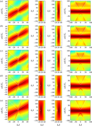
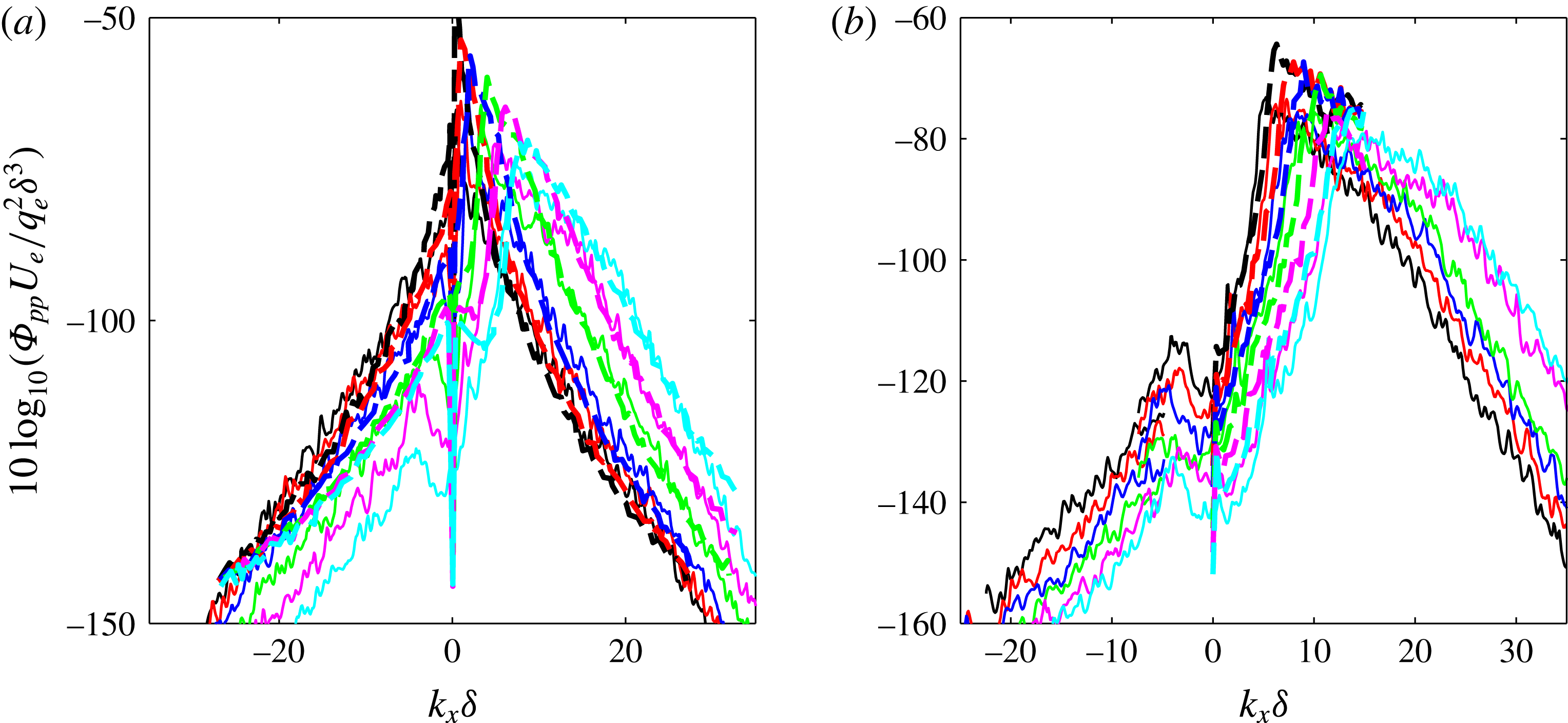
The temporal and spatial properties of wall-pressure fluctuations can be expressed in terms of wavenumber vector–frequency spectrum, which is the preferred input of vibroacoustic codes to predict the fluid–structure coupling. This spectrum is characterized by two main regions: the convective peak which represents the hydrodynamic signature of turbulent structures convected in the TBL, and the acoustic domain which encloses the supersonic wavenumbers, which are capable of radiating acoustic waves.
Due to its practical importance, several models for wavenumber–frequency spectrum have been proposed, e.g. Corcos (Reference Corcos1964), Witting (Reference Witting1986), Chase (Reference Chase1987), Mellen (Reference Mellen1994), Smol’yakov (Reference Smol’yakov2006). A comparison between the models by Graham (Reference Graham1997) shows a great disparity in the subconvective region. Furthermore, only Chase’s model takes into account the acoustic domain, but the empirical constants to set the level are arbitrary since there is no experimental work that gives these values. It is also difficult to validate the rate of decay from the position of the convective peak, which is essential to obtain correct levels in the subconvective region. There are indeed few available experimental attempts to measure wavenumber–frequency spectra (Wills Reference Wills1970; Blake & Chase Reference Blake and Chase1971; Panton & Robert Reference Panton and Robert1994; Abraham & Keith Reference Abraham and Keith1998; Ehrenfried & Koop Reference Ehrenfried and Koop2008; Arguillat et al. Reference Arguillat, Ricot, Robert and Bailly2010), and they are hardly reliable in the subconvective region. Moreover, they are restricted to zero-pressure-gradient TBL, with the exception of the recent work of Salze et al. (Reference Salze, Bailly, Marsden, Jondeau and Juvé2015).
When the wall is plane and it is assumed that the boundary layer is growing slowly, the pressure fluctuations can be considered statistically stationary in time and homogeneous in the streamwise (
 $x$
) and spanwise (
 $z$
) directions. For spatially developing boundary layers, the pressure is not homogeneous in the streamwise direction, but it is the commonly used assumption to obtain a frequency–wavenumber spectrum over a limited area. To that end, a triple transform is realized as follows: first a simple fast Fourier transform is applied in the
 $z$
-direction, which is periodic. Then a Welch’s algorithm is implemented for the time dimension: three overlapping segments of 4000 samples are used from the 8000 samples stored every 30 iterations of the LES. Each segment is weighted by a Hann window to reduce spectral leakage. To enhance the resolution for the
 $x$
-dimension, which is critical due to its limited extent, we rely on the spectral estimator of Capon (Reference Capon1969), given by
 $$\begin{eqnarray}\hat{P}_{Capon}(\unicode[STIX]{x1D714},k_{x},k_{z})=\frac{n_{x}+1}{\boldsymbol{e}^{H}(k_{x})R_{pp}^{-1}(\unicode[STIX]{x1D714},k_{z})\boldsymbol{e}(k_{x})},\end{eqnarray}$$
with
 $\boldsymbol{e}(k_{x})=(1\text{e}^{\text{i}k_{x}}\cdots \text{e}^{\text{i}k_{x}(n_{x}-1)})^{T}$
the stirring vector.
 $R_{pp}^{-1}$
is the inverse of the autocorrelation matrix, which has Toeplitz form and is inverted with a Cholesky method. To avoid ill-conditioning, the modified covariance method of Kay (Reference Kay1988) is used to estimate the autocorrelations. Note that the Hann window is also applied in
 $x$
-direction to reduce spectral leakage. Normalized two-sided spectra
 $\unicode[STIX]{x1D6F7}_{pp}(k_{x},k_{z},\unicode[STIX]{x1D714})$
are presented. The frequency resolution is the same as that for autospectra, namely
 $\unicode[STIX]{x0394}\unicode[STIX]{x1D714}\simeq 2.1\times 10^{-3}U_{\infty }/h$
. The wavenumber resolution is
 $\unicode[STIX]{x0394}k_{x}=2\unicode[STIX]{x03C0}/L_{x}=0.0035/h$
for the ZPG case and
 $0.0042/h$
for other cases, and
 $\unicode[STIX]{x0394}k_{z}=2\unicode[STIX]{x03C0}/L_{z}=0.025/h$
for the ZPG case and
 $0.027/h$
for other cases. Furthermore, normalization factors for compensating the windowing in time and
 $x$
-direction are applied. We check that a triple integration of
 $\unicode[STIX]{x1D6F7}_{pp}$
yields the mean pressure levels, obtained either directly or by integration of autospectra (4.1):
 $$\begin{eqnarray}\overline{p^{2}}=\int _{-\infty }^{\infty }\int _{-\infty }^{\infty }\int _{-\infty }^{\infty }\unicode[STIX]{x1D6F7}_{pp}(k_{x},k_{z},\unicode[STIX]{x1D714})\,\text{d}k_{x}\,\text{d}k_{z}\,\text{d}\unicode[STIX]{x1D714}.\end{eqnarray}$$
Slices of the frequency–wavenumber spectrum
 $\unicode[STIX]{x1D6F7}_{pp}(k_{x},k_{z},\unicode[STIX]{x1D714})$
are shown in figure 16 with outer scaling. Similar features are observed for the five gradients. The
 $k_{x}$
-
 $\unicode[STIX]{x1D714}$
slices clearly exhibit the antisymmetrical convective ridges, which is the imprint of the vortical structures populating the boundary layer. The white dashed line represents a mean convection speed
 $U_{c}=0.7U_{e}$
, which is in good agreement with the slope observed in the different cases, at least for low wavenumbers, i.e. large scales. The asymmetry with respect to this dashed line is related to the fact that the advection speed depends on the size of a given structure and on its altitude in the layer. In this representation, supersonic wavenumbers
 $k=\sqrt{k_{x}^{2}+k_{z}^{2}}<\unicode[STIX]{x1D705}_{0}=\unicode[STIX]{x1D714}/c_{\infty }$
define what we call the acoustic domain. This simple relationship has to be modified to take the mean flow into account. Supersonic wavenumbers then satisfy
 $(\unicode[STIX]{x1D705}_{0}-k_{x}M)^{2}-(k_{x}^{2}+k_{z}^{2})>0$
, where
 $M$
is the Mach number. The boundary of the acoustic domain is a slanted cone, which is represented in figure 16 by the solid white lines. At the centreline of the cone, for
 $k_{z}=0$
(first column), the half-line in the same direction as the convective ridge represents acoustic waves propagating in the flow direction at the phase speed
 $U_{e}+c_{\infty }$
. In the five cases, a sharp peak is visible at this location. It can easily be identified thanks to the antisymmetry with respect to the null frequency, since the lines are only plotted in the upper half-space. In the vicinity of the half-line
 $U_{e}-c_{\infty }$
, it is difficult to identify a sharp peak, but rather a spread acoustic activity. The acoustic levels are discussed thereafter but we can already notice that levels are increasing from favourable to adverse conditions, at least with this normalization (a logarithmic colour scale is used and the range is the same for each panel in a column). The second and third columns of figure 16 show
 $k_{x}$
-
 $k_{z}$
slices for two non-dimensional frequencies,
 $\unicode[STIX]{x1D714}\unicode[STIX]{x1D6FF}/U_{e}=3$
and 12. In this representation, the convective ridges look like an elongated elliptical shape, whose major axis is in the spanwise direction. The centre of ellipses moves toward positive streamwise wavenumbers as the frequency increases, and corresponds to the convective wavenumber
 $k_{c}=\unicode[STIX]{x1D714}/U_{c}$
. The trace of the acoustic domain with mean flow included is the ellipse
 $$\begin{eqnarray}(k_{x}+\unicode[STIX]{x1D705}_{0}M/\unicode[STIX]{x1D6FD}^{2})^{2}/(\unicode[STIX]{x1D705}_{0}/\unicode[STIX]{x1D6FD}^{2})^{2}+k_{z}^{2}/(\unicode[STIX]{x1D705}_{0}/\unicode[STIX]{x1D6FD})^{2}=1,\end{eqnarray}$$
Wavenumber–frequency spectra
 $10\log _{10}(\unicode[STIX]{x1D6F7}_{pp}(k_{x},k_{z},\unicode[STIX]{x1D714})U_{e}/q_{e}^{2}\unicode[STIX]{x1D6FF}^{3})$
. Slices for
 $k_{z}=0$
(first column, colour scale between
 $-$
310 and
 $-$
70), for
 $\unicode[STIX]{x1D714}\unicode[STIX]{x1D6FF}/U_{e}=3$
(second column, colour scale
 $-$
260 to
 $-$
90),
 $\unicode[STIX]{x1D714}\unicode[STIX]{x1D6FF}/U_{e}=12$
(third column, colour scale
 $-$
260 to
 $-$
90) and for
 $k_{x}\unicode[STIX]{x1D6FF}=-10$
(fourth column, colour scale
 $-$
360 to
 $-$
110). (a) FPGs; (b) FPGw; (c) ZPG; (d) APGw; (e) APGs.

with centre
 $(-\unicode[STIX]{x1D705}_{0}M/\unicode[STIX]{x1D6FD}^{2},0)$
, major radius
 $\unicode[STIX]{x1D705}_{0}/\unicode[STIX]{x1D6FD}^{2}$
, and minor radius
 $\unicode[STIX]{x1D705}_{0}/\unicode[STIX]{x1D6FD}$
,
 $\unicode[STIX]{x1D6FD}=\sqrt{1-M^{2}}$
being the Prandtl–Glauert parameter. This ellipse, plotted in white in the figure, is merged in the convective crest for the lowest frequency (second column of figure 16), whereas it clearly identifies the acoustic domain for the highest frequency (third column). The acoustic peaks on the ellipse border will be better emphasized on individual cuts in figures 17–20. When plotting a slice for
 $k_{x}\unicode[STIX]{x1D6FF}\simeq -10$
in the fourth column of figure 16, the convective region that encompasses the spanwise extent is shifted downwards. The boundaries of the acoustic domain are branches of a hyperbola, and the levels in the lower and upper half-spaces are different due to the mean flow effects.
Scaling of wavenumber–frequency spectra
 $\unicode[STIX]{x1D6F7}_{pp}(k_{x},0,\unicode[STIX]{x1D714})$
for a frequency corresponding to
 $\unicode[STIX]{x1D714}\unicode[STIX]{x1D6FF}/U_{e}=12$
. Outer scaling with
 $\unicode[STIX]{x1D6FF}$
(a) and
 $\unicode[STIX]{x1D6FF}^{\ast }$
(b) as the length scale; mixed scaling (c) for the case APGs (


As discussed thereafter, the best comparison between the five gradients is done by using
 $\unicode[STIX]{x1D6FF}$
as length scale. Very similar plots are obtained for favourable and zero gradient cases, but the extent of the convective ridge seems larger for the APG cases in the frequency and in the longitudinal wavenumber directions. The
 $k_{x}$
–
 $k_{z}$
slices show that the aspect ratio of the elliptical shape is lower for APG conditions, which is consistent with the experimental trend (Salze et al.
Reference Salze, Bailly, Marsden, Jondeau and Juvé2015). In the present study, the aspect ratio is almost unaffected for favourable gradients. The scaling of the spectra is investigated in figure 17. First, outer scaling is used in (a,b) with
 $\unicode[STIX]{x1D6FF}$
and
 $\unicode[STIX]{x1D6FF}^{\ast }$
as the length scale respectively. The superiority of
 $\unicode[STIX]{x1D6FF}$
over
 $\unicode[STIX]{x1D6FF}^{\ast }$
takes place both for normalizing the maxima of the convective hump and for reducing its extent over wavenumbers. The two FPG and the ZPG results are very close, whereas a broadening is once again visible for APG results. Mixed scaling is tested in figure 17(c), where
 $u_{\unicode[STIX]{x1D70F}}$
and
 $\unicode[STIX]{x1D70F}_{w}$
are the velocity and pressure viscous scales and
 $\unicode[STIX]{x1D6FF}^{\ast }$
is the outer length scale. Note that
 $\unicode[STIX]{x1D6FF}$
is still retained for normalizing the wavenumber axis. Mixed scaling, which has been shown to be efficient for matching autospectra in the intermediate-frequency range, does a good job of matching the convective peak levels.
Wavenumber–frequency spectra
 $\unicode[STIX]{x1D6F7}_{pp}(k_{x},0,\unicode[STIX]{x1D714})$
for successive non-dimensional frequencies
 $\unicode[STIX]{x1D714}\unicode[STIX]{x1D6FF}/U_{e}=1$
(


 $\unicode[STIX]{x1D6F7}_{pp}(k_{x},k_{z},\unicode[STIX]{x1D714})$
for
 $\unicode[STIX]{x1D714}=0$
and
 $k_{x}\unicode[STIX]{x1D6FF}=-10$
for the case APGs (


The evolution of the quantitative levels for the hump corresponding to hydrodynamic fluctuations and for the acoustic peaks are better appreciated on the individual spectra of figure 18(a–e), where the non-dimensional frequency is increased from 1 to 25. It is first noted that the maxima of the convective crest diminish at the same rate for all gradients. With the normalization by
 $\unicode[STIX]{x1D6FF}$
, the slope of the decay in the subconvective region is decreasing from favourable to adverse pressure gradients. The slope is however approximately constant as the frequency increases for a given case. For the ZPG LES, we have compared wavenumber–frequency spectra with models of Corcos (Reference Corcos1964), Chase (Reference Chase1987), Mellen (Reference Mellen1994) and Smol’yakov (Reference Smol’yakov2006) (not show here for brevity) and none of the models are able to reproduce the dynamics in the subconvective range. Furthermore, none of available experimental databases up to now are reliable in this region due to measurement errors. Nonetheless when compared in figure 19 to spectra computed from DNS of turbulent channel flow where streamwise homogeneity is fulfilled (Viazzo et al.
Reference Viazzo, Dejoan and Schiestel2001; Hu et al.
Reference Hu, Morfey and Sandham2002, Reference Hu, Morfey and Sandham2006), our LES results exhibit the same decay rate. The decay rate in the spanwise direction is assessed by the cut along
 $k_{z}$
plotted in figure 18(f). The spectra are symmetrical between negative and positive wavenumbers since there is no mean flow and the flow is homogeneous in this direction. Furthermore, no influence of the pressure gradient is observed when
 $\unicode[STIX]{x1D6FF}$
is used as the length scale. Second, regarding the acoustic contribution, the peak corresponding to
 $U_{e}+c_{\infty }$
is well-defined for all gradients, whereas a diffuse bump can be distinguished at
 $U_{e}-c_{\infty }$
. This asymmetry between waves propagating in the same direction as the mean flow or in the opposite direction has been explained by propagation effects due to the high mean shear introduced by the boundary layer profile (see discussion in Gloerfelt & Margnat Reference Gloerfelt and Margnat2014). In other words, refraction effects attenuate sound waves propagating against the flow, whereas channelling effects reinforce high-frequency waves in the other direction. Furthermore, the absolute acoustic levels are slightly higher for TBL subjected to adverse gradients than to favourable ones.
Comparison of ZPG LES with turbulent channel flow simulations. (a) Comparison of
 $\unicode[STIX]{x1D6F7}_{pp}(k_{x},k_{z}=0,\unicode[STIX]{x1D714})$
with DNS of Hu et al. (Reference Hu, Morfey and Sandham2002) for non-dimensional frequencies
 $\{1;2.5;5;10;15;20\}$
, corresponding to
 $\unicode[STIX]{x1D714}\unicode[STIX]{x1D6FF}/U_{e}=\{0.28;0.71;1.41;2.83;4.24;5.65\}$
(for channel flow,
 $U_{e}=u_{max}=18.2u_{\unicode[STIX]{x1D70F}}/0.819$
). (b) Comparison of
 $\unicode[STIX]{x1D6F7}_{pp}(k_{x},k_{z}=0,\unicode[STIX]{x1D714})$
with LES of Viazzo et al. (Reference Viazzo, Dejoan and Schiestel2001) for non-dimensional frequencies
 $\unicode[STIX]{x1D714}\unicode[STIX]{x1D6FF}/U_{e}=\{4.39;5.24;6.01;6.94;7.79;8.64\}$
.

The acoustic peaks are prominently displayed in figure 20. The isocontours in the
 $k_{x}$
–
 $k_{z}$
plane in (a) allow for the proper identification of the acoustic domain, which is at the same location (
 $k_{x}\unicode[STIX]{x1D6FF}\sim -5$
) for the three gradients shown. Two spanwise spectra are provided in (b,c) which corresponds to cuts along
 $k_{z}$
in the upper and lower half-spaces in panels shown in the fourth column of figure 16 for
 $\unicode[STIX]{x1D714}\unicode[STIX]{x1D6FF}/U_{e}=\pm 50$
. The cut in the lower half-space (b) corresponds to prograde waves and shows that the acoustic peaks are slightly increasing from favourable to adverse conditions. Note that the mean levels in (b,c) are not the same for APGs and APGw due to the slower decay rate of the convective ridge. The second cut makes it possible to distinguish the peaks associated with the retrograde acoustic waves. In terms of relative levels, the picture is reversed with respect to prograde waves.
Slice of
 $\unicode[STIX]{x1D6F7}_{pp}(k_{x},k_{z},\unicode[STIX]{x1D714})$
in the
 $k_{x}$
–
 $k_{z}$
plane (a) for
 $\unicode[STIX]{x1D714}\unicode[STIX]{x1D6FF}/U_{e}=12$
(four isocontour values of
 $10\log _{10}(\unicode[STIX]{x1D6F7}_{pp}(k_{x},k_{z},\unicode[STIX]{x1D714})U_{e}/q_{e}^{2}\unicode[STIX]{x1D6FF}^{3})$
in
 $\{-153,-133,-103,-91\}$
). Cuts of
 $\unicode[STIX]{x1D6F7}_{pp}(k_{x},k_{z},\unicode[STIX]{x1D714})$
for
 $k_{x}\unicode[STIX]{x1D6FF}=-10$
and
 $\unicode[STIX]{x1D714}\unicode[STIX]{x1D6FF}/U_{e}=-50$
(b) and 50 (c). Simulation APGs (


4.3 Direct noise levels
Another original point in our simulations is that the aeroacoustic emissions from the TBLs can be obtained directly. The radiated sound field is visualized in figure 21 on the non-rotated mesh (see § 2.2) using the same colour scale. Similar features are observed in all gradient cases. The most striking point is the very low levels, approximately 1 to 2 Pa for
 $p_{rms}$
. This is only 0.01 % of the inlet dynamic pressure
 $0.5\unicode[STIX]{x1D70C}_{\infty }U_{\infty }$
, justifying the great care taken to apply silent boundary conditions. A closer inspection would show that the radiated field is not totally free of spurious noise due to the inlet forcing or due to weak reflections at the outlet. But we are confident that the wavefronts shown in figure 21 do represent direct noise from wall turbulence. Low-frequency waves preferentially oriented in the direction opposite to the mean flow are visible for all cases. The particular directivity has been mainly explained by the convection effect at Mach around 0.5 (Gloerfelt & Berland Reference Gloerfelt and Berland2013). The Doppler effect for a compact source indeed decreases the wavelength upstream of the source, and conversely increases it downstream. This is accompanied by a rise of pressure levels upstream. The wavefronts have consequently a very large apparent wavelength and low levels downstream of the source.
Instantaneous views of the fluctuating pressure in the median plane of the non-rotated domain for APGs (a), APGw (b), ZPG (c), FPGw (d) and FPGs (e). Colour scale between
 $-$
3 and 3 Pa for each panel. The white bullet indicates the location where the spectra of figure 22 are evaluated.

A quantitative comparison between the different simulations is provided by the power spectral densities of the fluctuating pressure at the same physical height
 $y/h=408$
located in the acoustic field, plotted in figure 22. The so-called reflection theorem of Powell (Reference Powell1960) predicts that dipolar source terms in the acoustic analogy formulation of Curle (Reference Curle1955) degenerate toward quadrupolar sources when placed nearby an infinite plane, if viscous term sources can be neglected. By varying Mach number for a ZPG boundary layer, we have checked in Gloerfelt & Margnat (Reference Gloerfelt and Margnat2014) that integrated acoustic intensities follow a eighth power law of the free stream velocity, characteristic of quadrupolar source terms in the theory of Lighthill (Reference Lighthill1952). The statement of Powell (Reference Powell1960) is thus verified for boundary-layer noise. The first implication is that the aeroacoustic sources are rather inefficient, as for free turbulence. Second, the
 $U^{8}$
-dependency of the acoustic power can be used as scaling law for comparing the different gradient cases, which experience accelerations or decelerations of the free stream flow for FPG and APG conditions, respectively
 $+$
15 % for FPGs and
 $-$
9 % for APGs compared to the inlet velocity
 $U_{\infty }$
. In the dimensional analysis of Lighthill (Reference Lighthill1952)
 $p^{\prime }\propto \unicode[STIX]{x1D70C}U^{2}M^{2}$
, thus the pressure scale for non-dimensionalizing power spectra is
 $\unicode[STIX]{x1D70C}_{\infty }U_{e}^{2}M^{2}$
, where the Mach number is
 $M=U_{e}/c_{\infty }$
. Since the physical length of the plate is the same for all cases, a global time scale is used in figure 22(a), namely
 $h/U_{\infty }$
. The broadband nature of the frequency content is clearly depicted, and spectral shape and levels are similar, in particular for medium frequencies. Acoustic emissions are slightly increasing from favourable to adverse conditions with a broader range of high frequencies for APGs. This can be related to the higher Reynolds number obtained as the TBL grows thicker. It is even more visible when outer scaling by
 $\unicode[STIX]{x1D6FF}/U_{e}$
is used in figure 22(b), since
 $\unicode[STIX]{x1D6FF}$
is increasing from FPG to APG conditions.
Power spectral densities of fluctuating pressure at location
 $y=408h$
and
 $x=1630h$
for cases APGs (


 $x=1244h$
for ZPG (

 $h/U_{\infty }$
(a) and pulsation normalized by
 $\unicode[STIX]{x1D6FF}/U_{e}$
(b).

Comparison with DNS of Na & Moin (Reference Na and Moin1998): mean
 $\overline{u}$
profile (a), defect law (b) and turbulent intensities for FPG (c) and APG (d) conditions. FPG corresponds to station
 $x=0.5$
(experiment


 $x=0.85$
(experiment


 $x=0.5$

 $x=0.6$

 $x=0.7$

 $x=0.8$

 $x=0.85$


Comparison with measurements of Salze et al. (Reference Salze, Bailly, Marsden, Jondeau and Juvé2014): mean
 $\overline{u}$
profile (a), defect law (b) and turbulent intensities
 $u_{rms}$
(c) for cases APG25 (


5 Discussion and conclusions
A numerical experiment has been carried out to investigate the effects of an external pressure gradient on the fluctuating surface pressure beneath a turbulent boundary layer. This issue is a key driver of the flow-induced noise when a body moves through a fluid, and is present in a wide variety of applications. This topic has gained renewed interest with the reduction of other sources of noise, and thanks to new opportunities offered by recent advances in measurement techniques and numerical capabilities. A thorough comparison with the few available databases, where this subject is tackled, has been conducted to assess the state of the art. In particular, three recently published experimental data sets by Salze et al. (Reference Salze, Bailly, Marsden, Jondeau and Juvé2014), Catlett et al. (Reference Catlett, Anderson, Forest and Stewart2016) and Hu & Herr (Reference Hu and Herr2016) have been compared for the first time. In addition to bringing out pertinent points, we provided new and additional information about two important topics. First, a wavenumber–frequency analysis was realized, highlighting the dynamics in the subconvective region, which is particularly difficult and tedious to predict in measurements. Secondly, we could provide for the first time the acoustic contribution in the presence of a free stream pressure gradient and the levels of direct noise produced by the wall turbulence by solving directly the compressible Navier–Stokes equations for a Mach number close to 0.5.
In order to achieve this objective, large-eddy simulations (LES) were performed for low Reynolds number nearly equilibrium TBLs subjected to five moderate pressure gradients: two adverse gradients, referred to as APGs for the strongest gradient and APGw for the weakest one, two favourable gradients, relatively strong FPGs and weak FPGw, and a zero-pressure-gradient TBL, which serves as reference. LES helped us obtain the surface pressure on large domains, which is needed to achieve a satisfying wavenumber resolution. This approach is limited to relatively low Reynolds numbers, with respect to values encountered in wind-tunnel experiments or applications. The simulations are however a powerful tool to cope with the principal limitations and uncertainties of experimental work arising from the response of pressure sensors. The boundary-layer properties were analysed and compared carefully to published literature to assess the quality of LES and to evaluate the equilibrium character of the TBLs. The similarity of the mean and fluctuating velocity profiles is a favourable point to define frequency–wavenumber spectra but a spatially developing boundary layer is not homogeneous in the streamwise direction due to its thickening. This limitation is ignored to obtain frequency–wavenumber spectra and would deserve further investigations. The use of space-varying wavevector–frequency spectra (Strawderman Reference Strawderman1987) or spatial empirical mode decomposition (Debert et al. Reference Debert, Pachebat, Valeau and Gervais2011) could help to clarify this hypothesis. Another critical point to get the acoustic contribution is to avoid creating excessive noise in the numerical set-up. Since sources adjacent to a plane are of quadrupolar type as for free turbulence, direct noise emissions are rather inefficient and yield very low levels, which should not be lost in extraneous noise. For this reason we developed a specific strategy to trigger turbulence generating minimal spurious noise. Furthermore, non-reflecting boundary condition were coupled with large buffer layers at the upper and outlet boundaries to damp spurious reflections. Thanks to this apparatus, we were able to obtain the direct noise radiation from the TBLs. It also gave confidence in the results for the acoustic domain in the frequency–wavenumber analysis, that is to say the region of supersonic wavenumbers corresponding to the aeroacoustic component of the wall pressure.
The main outcomes about the influence of a pressure gradient on wall pressure are summarized. The best scales to obtain a similarity of mean and fluctuating velocity profiles were found to be the boundary-layer thickness
 $\unicode[STIX]{x1D6FF}$
and the velocity of Zaragola & Smits (Reference Zaragola and Smits1997),
 $U_{ZS}=U_{e}\unicode[STIX]{x1D6FF}^{\ast }/\unicode[STIX]{x1D6FF}$
. Several parameters can be defined to characterize the intensity of the pressure gradient based on outer, inner or mixed quantities. They were approximately constant on the region of interest for analyses, but did not describe unambiguously the flow since other parameters, such as the Reynolds number, the Mach number (compressibility effects) or the flow history, come into play, making comparisons across studies difficult. That is why it was not obvious to find a scaling for wall-pressure power spectral densities that relies on these quantities. Three classical scalings were tested. The outer scaling was found to be the most efficient to match the results for the different gradients in a wide range of frequencies, from low to medium ones. Very good compliance with the available databases was also observed, even if a weak Reynolds number dependence was noted for the spectral levels in the medium-frequency range. The mixed scaling, where the wall shear stress replaces the dynamic pressure as the pressure scale, was efficient to attenuate the Reynolds number dependence, but the different gradients then corresponded to distinct curves, with levels increasing from FPG to APG conditions. It is worth noting that the slope observed for the decay at the intermediate frequencies was higher for adverse gradients. The slopes were in fair agreement with recent measurements of Salze et al. (Reference Salze, Bailly, Marsden, Jondeau and Juvé2014), but they depend on the Reynolds number, which is too low in the simulations to draw firm conclusions or attempt to interpret their values. Inner scaling can be used to superimpose the spectra at very high frequencies representative of the viscous–dissipative scales for a given value of the pressure gradient. The roll-off part, sometimes approximated by a
 $\unicode[STIX]{x1D714}^{-5}$
-law, was shifted toward higher frequencies from favourable to adverse conditions. This hierarchy was visible in the LES results, even if the grid cut-off entailed a more rapid fall. As a consequence, some energy was lost in the calculations in the high-frequency range. This is not critical since the behaviour of viscous scales can be considered as quasi-universal. It was possible to reconstruct the lost energy by matching a model of Goody (Reference Goody2004), and we found a correction of 9 % of the averaged pressure fluctuations in the ZPG case. The integrated value scaled by the wall shear stress increased from FPG to APG conditions. This is consistent with experiments, but there is a lack of data to see an emerging trend with the value of a pressure-gradient parameter. The influence of the pressure gradient on the convective velocity of pressure fluctuations on the wall was not very conclusive. The view of Schloemer (Reference Schloemer1967) or Burton (Reference Burton1973) of a lower convection speed for APG flows and a higher one for FPG flows was not supported by the present numerical experiments, where Mach and Reynolds numbers are roughly constant for nearly equilibrium TBLs. Instead, the conclusion here was that the mean convective velocity from space–time correlations is weakly affected by the pressure gradient, except that the range of longitudinal separations scaled by the boundary layer thickness was reduced for APG flows due to the thickening of the TBL. The investigation of frequency-dependent convection velocities from cross-spectral measurements would help to establish a clearer trend. Furthermore, high-resolution wavenumber–frequency spectra were obtained and made clear the features of the convective ridge, which is the imprint of hydrodynamic pressure fluctuations associated with vortical motions, and of the acoustic domain, corresponding to boundary-layer noise. In particular, it was found that the boundary-layer thickness
 $\unicode[STIX]{x1D6FF}$
was the best length scale to compare the different gradient cases, even if an enlargement was visible for APG conditions in the frequency and streamwise wavenumber directions. As a result, the convective ridge was more isotropic in adverse conditions, which is consistent with the picture of hairpin structures that lift off the wall. The decay rate toward the subconvective wavenumbers revealed a large dynamical range, which is hardly reproduced in available modelling or in experiments. The trace of acoustic wavenumbers was clearly identifiable and showed slightly higher acoustic activity for APG boundary layers, at least when scaled with outer properties. This is consistent with the levels of direct radiation outside the TBL. The radiation patterns were similar for the five gradient cases and were significantly marked by mean flow propagation effects, which will be further analysed in a future paper.
Acknowledgements
This research has been funded by the Agence Nationale de la Recherche through the ANR-2011-BS09-035-01 project SONOBL. The authors also acknowledge Alois Sengissen and the support of Airbus SAS. This work was granted access to the HPC resources of IDRIS and CCRT under the allocation 2014-1736 made by GENCI (Grand Equipement National de Calcul Intensif). We also acknowledge PRACE (Partnership for Advanced Computing in Europe) for awarding us access to resource Curie TN based in France at TCGG under the allocation 2014102334.
Appendix A. Comparisons with experimental databases
This appendix contains comparisons with some existing databases dealing with wall-pressure fluctuations in the presence of pressure gradients.
Parameters for DNS of Na & Moin (Reference Na and Moin1998), taken from experiments of Watmuff (Reference Watmuff1988).
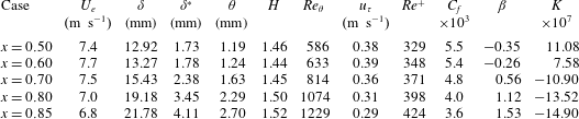
A.1 Comparisons with DNS of Na and Moin
Na & Moin (Reference Na and Moin1998) carried out DNS to study wall-pressure fluctuations with adverse pressure gradient and separation. We discuss their results that reproduce the experiments of Watmuff (Reference Watmuff1988), also documented and simulated by DNS in Spalart & Watmuff (Reference Spalart and Watmuff1993). Na & Moin (Reference Na and Moin1998) used an incompressible Cartesian code with an adjusted mean vertical velocity distribution on the top boundary to reproduce the pressure gradients in the converging–diverging channel used by Watmuff (Reference Watmuff1988). Thanks to the low Reynolds number, the flow was accurately simulated by the DNS of Spalart & Watmuff (Reference Spalart and Watmuff1993) and Na & Moin (Reference Na and Moin1998) (
 $\unicode[STIX]{x0394}x^{+}=16.6$
and
 $\unicode[STIX]{x0394}z^{+}=4.8$
). The flow parameters for the stations where the boundary layer is subjected to a mild favourable to adverse gradient are reported in table 3. The comparisons with the velocity field in figure 23(a–d) used the database of Spalart & Watmuff (Reference Spalart and Watmuff1993), made available on the web. The profiles of both experiment and DNS of Spalart & Watmuff (Reference Spalart and Watmuff1993) are plotted at non-dimensional station
 $x=0.60$
for the favourable case and at
 $x=0.85$
for the adverse case. Very good compliance is observed for the mean profile and turbulent intensities with the favourable gradient between experiments and DNS and between results of Spalart & Watmuff (Reference Spalart and Watmuff1993) and LES results FPGs. The adverse configuration is close to the APGs LES, with slight discrepancies for the wake parameter and near the peak of streamwise velocity fluctuations, essentially because the boundary layer is not in equilibrium in the experimental set-up and the adverse gradient changes. Power spectra from Na & Moin (Reference Na and Moin1998) for the stations between
 $x=0.5$
and 0.85 are compared with the different LES in figure 23(e,f). To match the low values of the Reynolds number in experiment/DNS, the LES spectra are computed at the beginning of the area of interest (i.e. at
 $x/h=1300$
for the ZPG LES and at
 $x/h=1500$
for the other cases). Data appear to collapse at low and intermediate frequencies, and the spectral roll-off is in fair agreement, even if the slopes are different since viscous dissipation implies a decrease following roughly a
 $\unicode[STIX]{x1D714}^{-5}$
law in DNS whereas the spatial cut-off of LES entails a more rapid fall. The spectra are presented with inner scaling in figure 23(f). The trends are similar but the effect of the different gradients is more pronounced in LES. This can be related to the more progressive variations of the friction velocity
 $u_{\unicode[STIX]{x1D70F}}$
in DNS since the non-equilibrium boundary layer evolves quickly from favourable to adverse conditions.
A.2 Comparisons with SONOBL experiments
The experiments realized in the framework of the SONOBL project by Salze et al. (Reference Salze, Bailly, Marsden, Jondeau and Juvé2014, Reference Salze, Bailly, Marsden, Jondeau and Juvé2015) were conducted in the main subsonic wind tunnel of the Centre Acoustique at Ecole Centrale de Lyon. The boundary layer was measured on the flat bottom wall of a test channel, with a length of 4 m, a height
 $h=0.25~\text{m}$
and a width
 $2h$
, opening in an anechoic chamber. The side walls were treated using a wire mesh and a porous liner to reduce noise generated at the channel outlet. An adjustable ceiling made of two flat plates was used to obtain both favourable and adverse pressure gradients. Hot-wire anemometry was used for the aerodynamic characterization. To measure cross-spectra and obtain frequency–wavenumber spectra, an antenna was designed by using a line of 63 remote microphones
 $(1/4~\text{in})$
on a flush-mounted disk, whose rotation makes it possible to have a two-dimensional exploration of wall pressure. A similar antenna was used in Arguillat et al. (Reference Arguillat, Ricot, Robert and Bailly2010). Wall-pressure spectra were measured with pinhole-mounted microphones (
 $1/8~\text{inch}$
Brüel and Kjaer type 4138 microphone with a cap hole diameter
 $d=0.5~\text{mm}$
). The observed Helmholtz resonance of the cavity below the pinhole was 21 kHz and the calibration was efficient from 10 Hz to 50 kHz. The configuration selected for comparisons are described in table 4, where the last column is the sensor diameter in wall units
 $d^{+}=\text{d}u_{\unicode[STIX]{x1D70F}}/\unicode[STIX]{x1D708}$
. Forest (Reference Forest2012) suggested that the dimensionless pinhole diameter
 $d^{+}$
should be smaller than 18 to ensure no sensor attenuation occurred for frequencies up to
 $\unicode[STIX]{x1D714}^{+}=1$
. The development of sensors based on microelectromechanical systems (MEMS) (Löfdahl, Kalvesten & Stemme Reference Löfdahl, Kalvesten and Stemme1996; Löfdahl & Gad-el Hak Reference Löfdahl and Gad-el Hak1999; White et al.
Reference White, Krause, De Jong, Holup, Gallman and Moeller2012) is a possible way to obtain very small sensors with
 $d^{+}<10$
. In SONOBL experiments,
 $d^{+}\sim 45$
and Corcos correction was used to obtain the autospectra up to
 $\unicode[STIX]{x1D714}^{+}=2$
.
Parameters of the experimental database of Salze et al. (Reference Salze, Bailly, Marsden, Jondeau and Juvé2014).
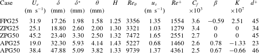
The mean and root-mean-square streamwise velocity profiles are in good agreement with LES profiles in figure 24(a–c), keeping in mind that the Reynolds numbers are two to three times higher in experiments. The adverse case is close to the APGw simulation, which is coherent with the value found for the pressure-gradient parameter
 $\unicode[STIX]{x1D6FD}$
. Wall-pressure autospectra are compared with outer, mixed and inner scalings in figures 24(d) to 24(f), respectively. The agreement in the low- and medium-frequency range are very good. The slightly lower levels of the experiments in outer scaling are related to the Reynolds number influence. The slopes obtained in the overlap region are compatible, even if the extent is reduced in the low Reynolds number simulations (approximately from
 $\unicode[STIX]{x1D714}\unicode[STIX]{x1D6FF}^{\ast }/U_{e}=0.5$
to 2 for adverse cases and from
 $\unicode[STIX]{x1D714}\unicode[STIX]{x1D6FF}^{\ast }/U_{e}=0.4$
to 1 for zero gradient). The slopes, added in figure 24(e), correspond to
 $\unicode[STIX]{x1D714}^{-1.2}$
for APGs;
 $\unicode[STIX]{x1D714}^{-0.8}$
for APGw;
 $\unicode[STIX]{x1D714}^{-0.5}$
for ZPG and
 $\unicode[STIX]{x1D714}^{-0.2}$
for FPGs. The green dashed line is the slope
 $\unicode[STIX]{x1D714}^{-5}$
often used to model viscous dissipation at high frequencies. When scaled with inner variables, the autospectra have still good compliance in the mid-frequency range. In particular, the measures for the adverse cases are close to the mild APGw LES. The mismatch at the low frequencies is a Reynolds number effect, whereas the discrepancies at high frequencies is due to the too fast roll-off of LES spectra.
Comparison with measurements of Catlett et al. (Reference Catlett, Anderson, Forest and Stewart2016): wall-pressure autospectra in outer (a) and mixed (b) scaling (APG
 $7^{\circ }$
,
 $U_{\infty }=28~\text{ft}~\text{s}^{-1}$

 $7^{\circ }$
,
 $U_{\infty }=56~\text{ft}~\text{s}^{-1}$

 $7^{\circ }$
,
 $U_{\infty }=84~\text{ft}~\text{s}^{-1}$

 $12^{\circ }$
,
 $U_{\infty }=56~\text{ft}~\text{s}^{-1}$

 $12^{\circ }$
,
 $U_{\infty }=84~\text{ft}~\text{s}^{-1}$

 $17^{\circ }$
,
 $U_{\infty }=84~\text{ft}~\text{s}^{-1}$


Parameters of the experimental database of Catlett et al. (Reference Catlett, Anderson, Forest and Stewart2016): APG
 $7^{\circ }$
at
 $x=-0.204~\text{m}$
(
 $-$
8.034 in) for the three inflow velocities (28, 56,
 $84~\text{ft}~\text{s}^{-1}$
), APG
 $12^{\circ }$
at
 $x=-0.154~\text{m}$
(
 $-$
6.073 in) and
 $U_{\infty }=56,84~\text{ft}~\text{s}^{-1}$
and APG
 $17^{\circ }$
at
 $x=-0.106~\text{m}$
(
 $-$
4.156 in) and
 $U_{\infty }=84~\text{ft}~\text{s}^{-1}$
.
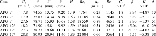
A.3 Comparisons with experiments of Catlett et al.
To investigate the effects of adverse pressure gradients on wall-pressure fluctuations, Catlett et al. (Reference Catlett, Anderson, Forest and Stewart2016) used flat airfoils with wedge-shaped trailing edges. The slopes of the wedge, corresponding namely to angles 7, 12 and
 $17^{\circ }$
, prescribe the value of the adverse gradient. The two-dimensional airfoils span the open jet test section, of width 2.44 m and height of roughly 1.5 m, of the anechoic flow facility at Naval Surface Warfare Center. A three-component hot-wire probe was used for the aerodynamic characterization and pinhole microphones are flush mounted to measure fluctuating pressure (Knowles Electronics model FG-23742-D36). The effective diameter of pinholes is 0.034 in (0.86 mm). The microphones have a flat frequency calibration curve up to the high-frequency limit of 7 kHz, which is above the physical limit. Thus, no Corcos correction is applied. Measurements are performed for three inflow velocities, 28, 56 and
 $84~\text{ft}~\text{s}^{-1}$
, and several locations on the inclined wall of the wedges. The selected cases for comparison are reported in table 5. We use the last but one station before the trailing where the gradient is well established, the value of
 $x$
being measured upstream of the trailing edge (
 $x=0$
). Power spectra are plotted in figure 25 with outer and mixed scaling. The three free stream velocities for
 $7^{\circ }$
-wedge give an indication of Reynolds number influence. The spectra for the two highest velocities compare favourably with APGw case when plotted with mixed scaling. The slope in the intermediate frequencies for
 $12^{\circ }$
-wedge is close to the one for APGs case, whereas the severe gradient corresponding to
 $17^{\circ }$
exhibits higher levels and a steeper slope. The Reynolds numbers in experiments of Catlett et al. (Reference Catlett, Anderson, Forest and Stewart2016) are three to ten times higher than the present simulations.
Comparison with measurements of Hu & Herr (Reference Hu and Herr2016): mean streamwise velocity profiles (a), plotted as a defect law (b) and in wall units (c) for adverse- (APG6


A.4 Comparisons with experiments of Hu and Herr
Hu & Herr (Reference Hu and Herr2016) conducted experiments in the open-jet anechoic test section (height 1.2 m
 $\times$
width 0.8 m) of the Acoustic Windtunnel Braunschweig. The TBL is measured on a flat wooden plate placed at mid-height and whose span is larger than the jet to reduce side-edge effects. Favourable to adverse gradients are explored by adjusting the rotation of a NACA0012 airfoil (chord 0.4 m), located just upstream of the plate bevelled trailing edge and at a distance 0.12 m above the plate. Three negative rotation angles,
 $-$
14,
 $-$
10 and
 $-6^{\circ }$
, yield three values for the adverse pressure gradient, and two positive angles, 12 and
 $14^{\circ }$
, set the intensity of the favourable gradients. Parameters reported in table 6 correspond to the most upstream measurement station,
 $x=1.21~\text{m}$
from the plate leading edge with the same inflow velocity
 $U_{\infty }=30.2~\text{m}~\text{s}^{-1}$
. Figure 26(a–c) presents the mean streamwise velocity profiles for the mild adverse (
 $\unicode[STIX]{x1D6FD}\simeq$
3.8) and favourable (
 $K\simeq 1.16\times 10^{-7}$
), which are closest to the LES flow conditions. Good agreement is observed even if, as explained by Hu & Herr (Reference Hu and Herr2016), the experimental set-up does not allow the establishment of equilibrium flows and the values of pressure-gradient and wake parameters are somewhat varying with respect to the measurement station. Wall pressure is measured with pinhole-mounted Kulite pressure transducers without the protection screen (model LQ-062-3.35bar, diameter
 $d=0.5~\text{mm}$
). The lowest frequency is imposed by the noise due to the open-jet free shear layer (
 ${\sim}230~\text{Hz}$
at
 $58.7~\text{m}~\text{s}^{-1}$
). The highest frequency is imposed by the electrical noise (
 ${\sim}7~\text{kHz}$
at
 $58.7~\text{m}~\text{s}^{-1}$
, which is below the Kulite-pinhole Helmholtz resonance frequency estimated at 30 kHz). No Corcos correction is applied. Wall-pressure spectra compared in figure 26(d–e) are also quite coherent with the findings of the present simulations. The levels of the different spectra have the same magnitude in the mid-frequency range when plotted using outer scales, and the mixed scaling allows to display the influence of the gradient with an increasing slope from favourable to adverse cases. The curve for APGs appears between those for APG6 and APG10, even if the value of
 $\unicode[STIX]{x1D6FD}$
is lower, but this parameter is dependent on flow history. The adverse gradient corresponding to the highest rotation angle
 $-14^{\circ }$
yields higher power levels and a steeper slope, coherently with the severe value of the gradient. The spectra for FPG cases are less sensitive to the precise value of the gradient. Intense fluctuations are however measured at the low frequencies and can be related to the particular experimental set-up.
Parameters of the experimental database of Hu & Herr (Reference Hu and Herr2016) at
 $x=1.21~\text{m}$
.