


1. Introduction
During the last years most economic studies have analysed the impact of environmental policies on international trade by means of the use of at least two-country general equilibrium models. However, because of their enormous simplifications of reality, their conclusions could lead policy makers to a misunderstanding of the true trade-offs between domestic and international competitiveness. In general, when we study the environmental issues associated with determined sectors of the economy, we often see that this kind of models fails to explain them. This emphasizes the need to work on partial equilibrium models to better understand such trade-offs. In particular, the latter are very useful when the polluting industries not only have the power to determine the domestic prices but also compete with some substitute goods which are imported from abroad.Footnote 1
In this context, the aim of this paper is to set up the theoretical framework that allows us to study the characteristics of environmental policy under these conditions. To accomplish this, we work in a two-good partial equilibrium model to design the environmental tax that maximizes the social welfare.Footnote 2 Furthermore, we assume that one of the goods is produced at home under non-competitive conditions, whereas another one, which is an imperfect substitute for the first, is imported from a foreign country. In addition, we assume that the price of the imported good is determined by the world market and that the distortion in production coexists with an environmental externality, where the latter comes from the pollutant emissions associated with the domestic production process. Finally, we rule out the possibility of trans-boundary environmental issues since they are not related to the small open economy condition. In a second extension to the literature, we allow for the possibility of innovation offsets and analyse how these can affect the level of the optimal environmental tax, where the strategic variable for the domestic firms is their investment in R&D.
Our results show that the optimal pollution tax can be expressed as the sum of a ‘domestic production effect’ and a ‘pollution effect’, where the first one stands for a decrease in social welfare because of the drop in domestic sales, and the second one constitutes an increase in social welfare as a result of the decrease in pollution damage. Therefore, depending on whether or not the ‘pollution effect’ surpasses the ‘domestic production effect’, the optimal policy represents a tax-cum-subsidy on pollution. In addition, when the domestic firms have the possibility of introducing innovation offsets via their investment in R&D, the optimal policy tax incorporates an ‘innovation effect’, whose impact on welfare depends on whether the new industry equilibrium (after the tax) is associated with higher or lower levels of emissions. Moreover, the introduction of innovation offsets can lead the economy to a win–win situation, implying that the sign of the optimal policy turns positive (i.e., we must introduce a pollution tax) and that there is a drop in the quantity imported of the foreign good. Finally, we conclude that, besides this situation, a comparison between the levels of this tax and the previous one (without innovation offsets) as well as their effects on the level of imports is not possible.
Turning to the analysis of the economic literature, we found no research addressing these concerns. As mentioned before, most analytical studies are based on the classical/neoclassical models of trade; besides that, non-competitive conditions respond to the use of environmental policy as strategic trade policy.Footnote 3
The remainder of this paper is organized as follows. Section 2 describes the basic model and establishes the optimal pollution policy that maximizes the social welfare. Section 3 sets out the pollution tax level when firms carry out endogenous R&D investments. The last section provides a summing-up and suggests some directions for further research.
2. The model
We place a two-stage game with two players to solve our regulation problem. Hence, working backward from the firms’ decisions to the government's tax decision, in the second stage, the producers choose their outputs and abatement levels under a Nash–Cournot behavioral assumption and, in the first stage, the government sets the tax on pollution to maximize social welfare, recognizing that both the equilibrium behavior of firms and the imports of the substitute commodity depend on the tax.
It should be noted that in the present context of a small open economy, the pollution (production) tax represents a first-best policy. However, we rule out the use of industrial policy on the assumption that environmental policy is politically more feasible than the previous one. Moreover, we assume that there is no interaction with other sectors of the economy, that the economy acts as a net-importer of the foreign good, and that the factor prices are given.Footnote 4, Footnote 5 Before proceeding, some general comments are in order. First, the paper is concerned with the effects of a specific pollution tax on emissions in a static context (i.e., a particular period of time), in which market structure, cost conditions and entry barriers are given. Second, we focus on industries where domestic firms sell in domestic markets but do not export the product. Third, working in a first-best policy leaves out the possibility of trade balance problems in the long run (i.e., the internalization of the environmental damage should improve the trade patterns and, therefore, the gains from trade). Finally, we work in a complete information model, where the government is assumed to know the demand structure of the firms’ output as well as their cost functions. Thus, it correctly anticipates the domestic firms’ output decisions given the imposed emission tax.
2.1 Domestic firms
The industry of the domestic good, x, consists of n identical firms, where the producing process generates a pollutant whose quantity depends on the level of production and abatement activities. Therefore, we can express the cost function for the firm as Cj(xj, aj), where xj and aj are the levels of production and abatement effort respectively. Also, we assume that Cj is increasing and strictly convex in its arguments, i.e., Cjx > 0, Cja > 0, Cjxx > 0, and Cjaa > 0 for all xj and aj, and that the level of emissions, ej, takes the following functional form: ej = ej(xj, aj), with ejx > 0, eja < 0, ejxa < 0, ejxx > 0, and ejaa > 0. Then, if Px(x, y, I) denotes the inverse demand function for x, with y and I representing the imported good and the monetary income respectively, in the second-stage game the representative firm chooses its output, xj, and abatement, aj, levels, recognizing that the rivals’ output and abatement levels as well as the environmental tax placed by the government, τ, are given, to maximize the following profit function:Footnote 6

which yields the first-order conditions


Aggregating, taking into account that the aggregate level of production of the domestic industry, x, is equal to x = nxj; of abatement, a, is equal to a = naj; and of emissions, e, is equal to e = nej; we can express the first-order conditions for the maximization of the profits at the industry level as:


where  .Footnote 7 Expression (3a) is a variant of the well-known equilibrium condition in Cournot models, stating that the Lerner index of any individual firm must be equal to that firm's market share divided by the absolute value of total-market-demand elasticity, whereas condition (3b) implies that firms abate pollution to the point where their marginal cost of reducing emissions equals the pollution tax.Footnote 8
2.2 Market equilibrium
Using (3a), we can express the equilibrium output for the domestic market as

Therefore, from (4), the response of the domestic output to a change in τ is given by

Note that as exa < 0, the sign of the second term in the numerator is determined by the effect of an increase in the level of abatement efforts on production costs, Cxa, which could be positive, zero, or negative, depending on the relation between these activities. In other words, the degree of complementarity between these processes will define the sign of the cross-partial derivative. Also, in the case of linear demand functions, Vxx = 0, the third term of the denominator, disappears from the expression. However, since  and primary effects (first derivatives) generally dominate secondary effects (second derivatives), the sign of (5) is assumed negative.Footnote 9
2.3 Social welfare and optimal policy
From the above, we can express the government revenues coming from the pollution tax on domestic emissions as τe. Therefore, if D(e) denotes the environmental damage resulting from any aggregate level of pollution in monetary terms, it is possible to define the social welfare function, SW, as the sum of (i) the consumer surpluses, (ii) the domestic industry profits, and (iii) the government revenues, less (iv) the pollution damage.

where Py(x, y, I) denotes the inverse demand function for y, Px, and Py represent the price of the domestic and imported good, respectively, and D(e) is assumed to be increasing and strictly convex, i.e., De > 0 and Dee > 0 for all e. This specification of aggregate social welfare avoids the issue of income distribution effects by weighting each welfare component equally; a way to modify it is to introduce an alternative weighting system. Hence, replacing in π(x.a) and e, we can rewrite (6) as

This provides a simple interpretation of the social welfare as the total benefits from consuming x and y less the private cost of producing x, the social cost of acquiring y (its domestic or international price), and the loss in consumer utility generated by the level of pollution. Then, turning to the analysis of the pollution tax that maximizes the social welfare, we find that in the first-stage game the government chooses the value of τ that maximizes (7), recognizing that y is a function of x and that x depends on τ. From (7), the effect on SW of a small change in τ is given by

Then, substituting in (8) for (3a) and (3b), we obtain the result that  when τ = τ*, where

with

The intuition behind this expression is as follows: The first term denotes the ‘domestic production effect’ and represents a decrease in the welfare of the society. That is, as x is a good whose marginal benefit to consumers (Px) exceeds its marginal cost (apart from the pollution cost), a higher τ decreases the amount of sales of the domestic firms and, therefore, the social welfare. On the other hand, the second term stands for the ‘pollution effect’ and constitutes an improvement in social welfare. Here, a higher τ results in a lower level of emissions, which improves the social welfare because of the decrease in the pollution damage. Also, note that as y is a negative function of x,  , a drop in the sales of the domestic firms augments the amount imported of the good y. Therefore, depending on whether or not the ‘pollution effect’ exceeds the ‘domestic production effect’, the optimal policy consists of a tax-cum-subsidy on pollution.
3. Endogenous R&D investments
The model described above provides a tractable framework to allow for the possibility of private actions to counteract the environmental tax effects. Here, we assume that the domestic producers can neutralize such effects through the introduction of some innovation offsets, where the strategic variable for the firms is the investment in R&D.Footnote 10 Hence, we need to focus on a three-stage game, where in the second-stage the producers choose their R&D expenditures required to employ a particular technology, and in the third-stage they choose their outputs and abatement levels. Hence, assuming that the total, average, and marginal costs are decreasing and convex in innovation expenditures, φj, and that the new technology reduces the production as well as the abatement costs, we can express the firm's total cost function as Cj(xj, aj, φj), with Cj φ < 0 and Cj φφ > 0 for all φj.Footnote 11, Footnote 12 Now, at the third-stage game the jth firm chooses its own output, xj, and abatement level, aj, recognizing that the emission tax, τ, set by the government in stage one, the level of φj set in stage two, φj*, and the output and abatement level of its rivals are given. This leads to the following first-order conditions for the domestic industry:


In the second-stage game, the representative firm maximizes its profits with respect to φj, assuming that the rivals’ expenditures on R&D are given. However, it figures out that its output and abatement level and the rivals’ output and abatement level in the next stage depend on φj. Therefore, it chooses φj to maximize

where the first-order condition at the industry level is given by

where φ and C φ are the level of innovation expenditures and the innovation marginal cost for the domestic industry respectively. Furthermore, the third term in the brackets represents the change in the market power of the domestic firms, an increase in φ decreases the cost of production per unit of output, which, since  increases the sales of x.
Since the derivation of an optimal value of innovation, φ*, in explicit form is impossible, we can obtain additional insights by taking the second-order condition for a maximum. Then, from (12) we obtain

where  is positive and C xφ and C aφ are negative by definition. Thus, as the terms in brackets above denote the demand and supply sides of the market, the effect of a change in φ on the market power of the domestic industry will be greater under linear demand functions (i.e., Vxx = 0) and complementary activities, Cxa > 0.Footnote 13
Finally, in the first-stage game, the government maximizes SW(τ) recognizing that x, y and φ all depend on τ. Therefore, the first-order condition for the government problem is

with  . Hence, using (10a) and (10b), the optimal tax pollution, τ**, can be written as

with

Comparing (9) with (15), we observe that the introduction of innovation offsets generate some distinctive characteristics in the expression for τ. Now, it is possible to reverse the conclusion that under non-competitive conditions the optimal policy should be a tax-cum-subsidy on pollution. To see this, note that when such offsets are added, the signs of the numerator and denominator of the ‘domestic production effect’ are undetermined, which implies the possibility that it can turn positive. In other words, this will happen when

or

with

The rationale behind this result is as follows: when the indirect effect generated by the innovation process surpasses the direct effect of τ on x and the denominator still remains negative, since the abatement effect dominates the production effect of τ on e, the introduction of innovation offsets not only increases the sales of x but also decreases the level of emissions, which, therefore, improves the social welfare. Also, note that as the domestic sales of x increase, there will be a drop in the quantity imported of good y. In contrast, if the direct effect dominates the indirect effect of τ on x (i.e., ρ < 0 with 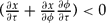 ), the ‘domestic production effect’ maintains its negative sign. In addition, the second term in (15) describes what we call the ‘innovation effect’: an increase in τ diminishes the production costs, which is welfare increasing when the new equilibrium for x is associated with a lower level of emissions, ρ < 0, or welfare decreasing when the contrary happens, ρ > 0. Hence, we observe that under a win–win situation (i.e., when the firms can reduce their emissions level and increase their domestic sales), the optimal policy represents a tax on pollution and has a higher level than the previous one (without innovation offsets), i.e., τ** > τ*, with τ** > 0, and τ* > = < 0.Footnote 14 Otherwise, if the innovation offsets are positively correlated with higher emissions (i.e., ρ > 0), we obtain that τ** could be lower or greater than τ*.
4. Conclusions
This paper focuses on the design of optimal environmental policy when non-competitive conditions exist in a small economy. To accomplish this, we work in a two-good partial equilibrium model, where one of the goods is imported from a foreign country. As the preceding analysis made clear, the optimal pollution policy under domestic distortions can be decomposed into a ‘domestic production effect’, which describes the change in welfare coming from a variation in the level of domestic firms’ sales, and a ‘pollution effect’, capturing the change in welfare coming from a variation in pollution damage. Furthermore, since these two effects have opposite signs, the optimal policy will be a tax-cum-subsidy on pollution, depending on whether or not the ‘pollution effect’ dominates the ‘domestic production effect’.
Interesting highlights appear when the firms have the possibility of introducing innovation offsets through their investment in R&D. In this case, the optimal pollution tax adds an ‘innovation effect’, which captures the change in welfare coming from a decrease in production costs. From the analysis, its effect on welfare will depend on whether the new equilibrium (after the tax) for the domestic industry is associated with a higher or lower level of emissions, creating the possibility that we can obtain a win-win situation when the innovation offsets generate more abatement than emissions and the domestic firms increase their sales. Finally, we conclude that only under a win-win situation does the optimal environmental policy represent a tax and it is higher than the previous one (without innovation offsets). Otherwise, a comparison between them is impossible.
There are many additional areas of research that could be pursued. A natural extension would be to admit the presence of foreign direct investment in the form of local production of the imported good. Another development would be to introduce stochastic elements.
 and
 when we work on the demand side of the market.
 .


