





%20--%3e%3c!DOCTYPE%20svg%20PUBLIC%20'-//W3C//DTD%20SVG%201.0//EN'%20'http://www.w3.org/TR/2001/REC-SVG-20010904/DTD/svg10.dtd'%3e%3csvg%20version='1.0'%20id='Layer_1'%20xmlns='http://www.w3.org/2000/svg'%20xmlns:xlink='http://www.w3.org/1999/xlink'%20x='0px'%20y='0px'%20width='64px'%20height='64px'%20viewBox='5.5%20-3.5%2064%2064'%20enable-background='new%205.5%20-3.5%2064%2064'%20xml:space='preserve'%3e%3cg%3e%3ccircle%20fill='%23FFFFFF'%20fill-opacity='0'%20cx='37.785'%20cy='28.501'%20r='28.836'/%3e%3cpath%20fill='%23595959'%20d='M37.441-3.5c8.951,0,16.572,3.125,22.857,9.372c3.008,3.009,5.295,6.448,6.857,10.314%20c1.561,3.867,2.344,7.971,2.344,12.314c0,4.381-0.773,8.486-2.314,12.313c-1.543,3.828-3.82,7.21-6.828,10.143%20c-3.123,3.085-6.666,5.448-10.629,7.086c-3.961,1.638-8.057,2.457-12.285,2.457s-8.276-0.808-12.143-2.429%20c-3.866-1.618-7.333-3.961-10.4-7.027c-3.067-3.066-5.4-6.524-7-10.372S5.5,32.767,5.5,28.5c0-4.229,0.809-8.295,2.428-12.2%20c1.619-3.905,3.972-7.4,7.057-10.486C21.08-0.394,28.565-3.5,37.441-3.5z%20M37.557,2.272c-7.314,0-13.467,2.553-18.458,7.657%20c-2.515,2.553-4.448,5.419-5.8,8.6c-1.354,3.181-2.029,6.505-2.029,9.972c0,3.429,0.675,6.734,2.029,9.913%20c1.353,3.183,3.285,6.021,5.8,8.516c2.514,2.496,5.351,4.399,8.515,5.715c3.161,1.314,6.476,1.971,9.943,1.971%20c3.428,0,6.75-0.665,9.973-1.999c3.219-1.335,6.121-3.257,8.713-5.771c4.99-4.876,7.484-10.99,7.484-18.344%20c0-3.543-0.648-6.895-1.943-10.057c-1.293-3.162-3.18-5.98-5.654-8.458C50.984,4.844,44.795,2.272,37.557,2.272z%20M37.156,23.187%20l-4.287,2.229c-0.458-0.951-1.019-1.619-1.685-2c-0.667-0.38-1.286-0.571-1.858-0.571c-2.856,0-4.286,1.885-4.286,5.657%20c0,1.714,0.362,3.084,1.085,4.113c0.724,1.029,1.791,1.544,3.201,1.544c1.867,0,3.181-0.915,3.944-2.743l3.942,2%20c-0.838,1.563-2,2.791-3.486,3.686c-1.484,0.896-3.123,1.343-4.914,1.343c-2.857,0-5.163-0.875-6.915-2.629%20c-1.752-1.752-2.628-4.19-2.628-7.313c0-3.048,0.886-5.466,2.657-7.257c1.771-1.79,4.009-2.686,6.715-2.686%20C32.604,18.558,35.441,20.101,37.156,23.187z%20M55.613,23.187l-4.229,2.229c-0.457-0.951-1.02-1.619-1.686-2%20c-0.668-0.38-1.307-0.571-1.914-0.571c-2.857,0-4.287,1.885-4.287,5.657c0,1.714,0.363,3.084,1.086,4.113%20c0.723,1.029,1.789,1.544,3.201,1.544c1.865,0,3.18-0.915,3.941-2.743l4,2c-0.875,1.563-2.057,2.791-3.541,3.686%20c-1.486,0.896-3.105,1.343-4.857,1.343c-2.896,0-5.209-0.875-6.941-2.629c-1.736-1.752-2.602-4.19-2.602-7.313%20c0-3.048,0.885-5.466,2.658-7.257c1.77-1.79,4.008-2.686,6.713-2.686C51.117,18.558,53.938,20.101,55.613,23.187z'/%3e%3c/g%3e%3c/svg%3e)
%20--%3e%3c!DOCTYPE%20svg%20PUBLIC%20'-//W3C//DTD%20SVG%201.0//EN'%20'http://www.w3.org/TR/2001/REC-SVG-20010904/DTD/svg10.dtd'%3e%3csvg%20version='1.0'%20id='Layer_1'%20xmlns='http://www.w3.org/2000/svg'%20xmlns:xlink='http://www.w3.org/1999/xlink'%20x='0px'%20y='0px'%20width='64px'%20height='64px'%20viewBox='5.5%20-3.5%2064%2064'%20enable-background='new%205.5%20-3.5%2064%2064'%20xml:space='preserve'%3e%3cg%3e%3ccircle%20fill='%23FFFFFF'%20fill-opacity='0'%20cx='37.637'%20cy='28.806'%20r='28.276'/%3e%3cg%3e%3cpath%20fill='%23595959'%20d='M37.443-3.5c8.988,0,16.57,3.085,22.742,9.257C66.393,11.967,69.5,19.548,69.5,28.5c0,8.991-3.049,16.476-9.145,22.456%20C53.879,57.319,46.242,60.5,37.443,60.5c-8.649,0-16.153-3.144-22.514-9.43C8.644,44.784,5.5,37.262,5.5,28.5%20c0-8.761,3.144-16.342,9.429-22.742C21.101-0.415,28.604-3.5,37.443-3.5z%20M37.557,2.272c-7.276,0-13.428,2.553-18.457,7.657%20c-5.22,5.334-7.829,11.525-7.829,18.572c0,7.086,2.59,13.22,7.77,18.398c5.181,5.182,11.352,7.771,18.514,7.771%20c7.123,0,13.334-2.607,18.629-7.828c5.029-4.838,7.543-10.952,7.543-18.343c0-7.276-2.553-13.465-7.656-18.571%20C50.967,4.824,44.795,2.272,37.557,2.272z%20M46.129,20.557v13.085h-3.656v15.542h-9.944V33.643h-3.656V20.557%20c0-0.572,0.2-1.057,0.599-1.457c0.401-0.399,0.887-0.6,1.457-0.6h13.144c0.533,0,1.01,0.2,1.428,0.6%20C45.918,19.5,46.129,19.986,46.129,20.557z%20M33.042,12.329c0-3.008,1.485-4.514,4.458-4.514s4.457,1.504,4.457,4.514%20c0,2.971-1.486,4.457-4.457,4.457S33.042,15.3,33.042,12.329z'/%3e%3c/g%3e%3c/g%3e%3c/svg%3e)
1. Introduction
The notion of ‘coherent structures’ in a turbulent flow goes back to Townsend (Reference Townsend1956), Grant (Reference Grant1958), Kline et al. (Reference Kline, Reynolds, Schraub and Runstadler1967) and others. It refers to organized motions that can be observed over time, but occur rather randomly in space and time, at least as long as the mechanisms behind them are not fully understood. Typical representatives of such ‘coherent structures’ are, for example, ‘eddies’, ‘shear layers’, ‘turbulent spots’, ‘bubbles (slugs)’ or ‘air blasts (puffs)’. Hussain (Reference Hussain1983) suggests that also the phase-correlated portion of the vorticity be called ‘coherent structure’, representing the largest spatial extent over which coherent vorticity exists. One of the most important properties of coherent structures is their Galilean invariance together with the requirement that they do not overlap each other. Hence, each structure has its own domain and boundary, although the volume or mass of a ‘coherent structure’ can change over time. A coherent structure can further consist of coherent substructures (e.g. hairpin vortices) and they can interact with other structures. The associated processes are nonlinear; see, e.g. Hussain (Reference Hussain1983). According to the latter definition, turbulence can thus be regarded as an unsteady process consisting of both coherent and phase random (i.e. incoherent) motions; the latter overlap with the former and generally extend beyond the boundaries of a coherent structure. Jiménez (Reference Jiménez2018) describes wall-bounded turbulence as a deterministic high-dimensional dynamical system of interacting coherent structures defined as vortices with sufficient internal dynamics to behave relatively independently of any remaining incoherent part of the flow. His central idea is that randomness is not a property, but a methodological decision about what to ignore in the flow. Accordingly, a complete understanding of turbulence – including the possibility of controlling it – requires that this randomness be minimized; see Jiménez (Reference Jiménez2018).
Traditionally, methods for detecting ‘coherent structures’ fall into two camps based on either the Eulerian or Lagrangian description of the flow considered. The first considers the flow field in a stationary, external coordinate system, while the second considers it in one that moves with the flow particles. The background of a possible dispute between the two camps is the demand for Galilean invariance of the results and the conclusions drawn. Conceptually, this can be most safely achieved with the Lagrangian approach. This approach offers the possibility of ‘objectively’ identifying structures that arise during the transport of material by a complex, unsteady flow motion, i.e. independent of the point of view of any observer. An excellent introduction to the history and current state of Lagrangian methods is given by Haller (Reference Haller2015). The basis of these methods is the so-called ‘flow map’, which maps particle positions at different times onto each other. Since particle-based flow visualizations strongly depend on the chosen starting positions of the particles in space and time, it is more suitable to consider the flow field deformations that are contained implicitly in the flow map as the selected initial position then loses its influence. While the effect of the time interval over which the integration was performed remains, this effect is considerably mitigated by the fact that motions belonging to coherent structures have a greater effect on the deformation of the fluid than the small-scale incoherent ones.
Based on the ‘flow map’, often either the finite-size Lyapunov exponent (FSLE) or the finite-time Lyapunov exponent (FTLE) is utilized to quantify and visualise the deformation; see Bettencourt, López & Hernández-García (Reference Bettencourt, López and Hernández-García2013) and Haller (Reference Haller2015), respectively. Both the FSLE and FTLE are practically equivalent and determine the maximum strain or compression of the fluid based on the maximum or minimum eigenvalues of the right Cauchy–Green strain tensor derived from the ‘flow map’. The physical interpretation of the eigenvalues depends on whether one traverses the flow forward or backward in time. Forward in time, the maximum and minimum eigenvalues represent the divergence and convergence of the fluid, respectively; see Haller & Sapsis (Reference Haller and Sapsis2011). For a negative time axis, the association simply reverses. The structures of maximum values observed in the FTLE fields form ‘barriers’ in the flow field, separating different regions. This can be observed particularly well in the wake of a two-dimensional bluff body (v. Kármán's vortex street), cf. e.g. Kasten et al. (Reference Kasten, Petz, Hotz, Hege, Noack and Tadmor2010), for which a line system of attracting and repelling attractors sets up, commonly referred to as ‘attracting Lagrangian coherent structures (LCS)’ and ‘repelling LCS’. Both lines intersect in the region of a so-called ‘hyperbolic LCS’, owing to the fact that material converging in one direction has to diverge in another direction (conservation of mass), cf. Haller (Reference Haller2015).
Applied to three-dimensional turbulent flows, the structures visualised in FTLE images have been associated with vortices in the flow field in numerous works, as shown by various comparisons between FTLE and Eulerian methods; see, e.g. Green, Rowley & Haller (Reference Green, Rowley and Haller2007), Pan, Wang & Zhang (Reference Pan, Wang and Zhang2009), Bettencourt et al. (Reference Bettencourt, López and Hernández-García2013) and Wilson, Tutkun & Cal (Reference Wilson, Tutkun and Cal2013). Compared with Eulerian methods, however, the resulting FTLE images have the aforementioned advantage of being Galilein invariant and revealing finer structures. Furthermore, they are more robust with respect to background noise or inaccuracies in the input data as well as in the computational method; compare, e.g. Haller (Reference Haller2015).
Through particle image velocimetry data of a turbulent boundary layer at a low Reynolds number ( $Re_{\theta }=481$), Pan et al. (Reference Pan, Wang and Zhang2009) identified LCS in a longitudinal section by reducing the data to their ridge lines. The results showed that the attracting LCS act like projections of hairpin vortices onto the plane. As a result, their inclination angles and phase velocities in different wall-normal positions are determined versus normalised wall distance
 $y^+$. As in Green et al. (Reference Green, Rowley and Haller2007), the robustness of the LCS along with its independence from thresholds and quantitative details that can be extracted from the field is confirmed.
In the work of Bettencourt et al. (Reference Bettencourt, López and Hernández-García2013), the FSLE is used to identify LCS in three-dimensional flows; a turbulent channel flow and an oceanic flow. The most attracting or repelling structures are detected based on the ridge lines of the FSLE field. In the turbulent channel flow the FSLE field is divided into longitudinal structures near the wall, which evolve into oblique structures away from the wall. Correlations in the streamwise and spanwise directions show the typical dimensions of these structures. They are found to resemble Eulerian coherent structures known to occur in the same regions of the turbulent channel. In particular, these are elongated vortices in the flow direction that move the fluid away from the wall into the core of the channel at low velocity. Three dimensionally, the LCSs appear as mushroom-shaped extensions of near-wall, layered structures whose size is comparable to the channel width. They separate the channel into an inner region, where the FSLE reaches high values, and an outer region with low FSLE values. The distribution of LCS in the turbulent channel resembles the commonly accepted picture where upward protrusions of near-wall fluid coexist with downward, rotation-free flows in the centre of the channel. Nevertheless, Bettencourt et al. (Reference Bettencourt, López and Hernández-García2013) concluded that further work is needed to clarify the relationships between LCS and fluid transport in this type of flow; not least because visualisation of three-dimensional structures and transport in turbulent flows is a complex and time-consuming topic.
However, regarding the notion of attracting and repelling LCS, it is to be mentioned that not every ridge line in an FTLE field automatically represents an LCS, as shown by some generic examples in, e.g. Haller (Reference Haller2015) or Farazmand & Haller (Reference Farazmand and Haller2012). A typical example is the strain of the fluid generated by pure shear, which does not lead to any local divergence or convergence of the fluid particles, despite representing a possible FTLE extreme value. In consequence, Farazmand & Haller (Reference Farazmand and Haller2012) developed a refined method for the detection of LCS in two-dimensional flows. This method has been used by Wilson et al. (Reference Wilson, Tutkun and Cal2013) to analyse their data in a wall-parallel slice of a flat-plate turbulent boundary layer after demonstrating that the third velocity component perpendicular to the slice can be considered negligible. The investigations were performed at  $Re_{\theta } = 9800$ and
 $y^+=50$. By comparison of the instantaneous flow field (minus mean flow in Eulerian terms) with the lines of repelling and attracting LCS, it is confirmed that the LCS segment the flow field. Furthermore, hyperbolic regions near the intersections of the two are illustrated and confirmed and local phenomena described as ‘spurts’, ‘swirls’ and ‘stagnations’ are tracked in time. In this way a more detailed insight into the instantaneous flow field is provided, going beyond the mere confirmation of the presence of vortices (see above). However, a connection of ‘spurts’ and ‘swirls’ to parabolic or elliptic LCS is not established. Interestingly, several groups of smaller adjacent segments were identified in the study, which form larger structures when viewed together – in the sense of the idea of coherent substructures described at the beginning – which do not overlap but complement each other. This gives hope that LCS or FTLE analyses could also contribute to the identification of turbulent large-scale structures.
Next to the ‘hyperbolic LCS’ that have been the focus so far, regions other than attracting and repelling LCS typically catch the eye in two-dimensional flows. These exhibit an FTLE minimum around which another type of transport barrier may exist. Haller (Reference Haller2015) and Farazmand, Blazevski & Haller (Reference Farazmand, Blazevski and Haller2014) call these regions ‘elliptic LCS’ and ‘parabolic LCS’. The former involve the fluid in the core region of a vortex rotating about a central axis in a manner similar to a solid. Since adjacent fluid particles remain together when rotating about a common axis, an FTLE minimum is present here and the FTLE value then increases with distance from the axis as frictional effects increase. Haller (Reference Haller2015), Haller et al. (Reference Haller, Hadjighasem, Farazmand and Huhn2016), etc. succeed in determining an invariant line for the objective boundary of the elliptic LCS. A comparison of different methods for segmenting two-dimensional flow fields is presented in Hadjighasem et al. (Reference Hadjighasem, Farazmand, Blazevski, Froyland and Haller2017). ‘Parabolic LCS’, in contrast, are found in the core of free jets; see, e.g. Haller (Reference Haller2015), Farazmand et al. (Reference Farazmand, Blazevski and Haller2014). These are associated with a minimum of shear and, thus, a minimal FTLE value, implying that particles stay together longer in the centre than at the edge of the jet or parabolic region. Phenomenologically, a connection to the ‘spurts’ in Wilson et al. (Reference Wilson, Tutkun and Cal2013) is conceivable, although this has not been examined in depth. Beron-Vera et al. (Reference Beron-Vera, Olascoaga, Brown, Koçak and Rypina2010) and Beron-Vera et al. (Reference Beron-Vera, Olascoaga, Brown and Koçak2012) identify the associated transport barriers in the minima of the forward and backward-integrated FTLE fields. However, they refer to them by the problem-specific term of an inertial torus, which fits their geophysical application but is not applicable to more general cases. It is obvious that this is the more general phenomenon of a parabolic LCS.
In a very recent study, Huang, Borthwick & Lin (Reference Huang, Borthwick and Lin2022) presented an investigation of LCS in two-dimensional unsteady CFD data of the flow past a backward facing step. A new feature in their work is a so-called ‘flow pathway’ with minimal FTLE values between vortices that is periodically opened and closed by FTLE ridges associated with the shedding of vortices. This flow pathway is identified by minimal FTLE values and due to this fact, the distances between neighbouring fluid particles within it only vary slighty.
2. Objectives of this study
As outlined above, the FTLE has become a commonly used tool in turbulent flow analysis in recent years. However, in the investigation of three-dimensional problems – and in contrast to two-dimensional ones – it is noticeable that the FTLE field has mostly been used for identification/illustration purposes of turbulent structures contained in the unsteady turbulent flow field. An exception is provided by the study of Wilson et al. (Reference Wilson, Tutkun and Cal2013), where one wall-parallel plane of a flat-plate turbulent boundary layer obtained from a wind tunnel experiment is investigated, motivating their suggestion that similar studies based on direct numerical simulation (DNS) should be performed with the full three-dimensional flow field. Thus, although the FTLE propagated by Haller (Reference Haller2001) allows the objective detection of structures in unsteady flow fields, cf. Haller (Reference Haller2015), it has not yet been used extensively to present in-depth analyses of three-dimensional turbulent boundary-layer flows. Consequently, proceeding from the present state, it is the main objective of this work to apply a Lagrangian method to high-resolution DNS data of a spatially evolving wall-bounded turbulent boundary layer – in contrast to previous channel flows – and, thus, to complement existing studies focusing on the maxima of the FTLE field. Hereby, the main objectives are: (i) to clearly characterise the dependence of the FTLE field from the wall-normal distance, (ii) to associate the structures observed in the FTLE field with turbulent motions within the unsteady turbulent field, (iii) by also looking at the minima in the FTLE field, to work out the meaningfulness of the usually less discussed regions of minimal FTLE values for the turbulent field. The starting point for this study are the DNS data of Wenzel et al. (Reference Wenzel, Gibis, Kloker and Rist2019) of self-similar turbulent boundary layers with a moderate adverse pressure gradient (APG) in the streamwise direction, which noticeably increases the Reynolds number range under consideration compared with data without a pressure gradient. Note that a comparison between studies of cases with and without pressure gradients did not show a substantial influence of the pressure gradient, which is why all the results shown apply in a comparable way to cases with and without pressure gradients; further details will be given at an appropriate position.
The reader interested in the influence of an APG on the statistical and kinematic characteristics of turbulent boundary layers may have a look at Houra, Tsuji & Nagano (Reference Houra, Tsuji and Nagano2000) for instance. Their study did not yet deliver a significant influence of the adverse pressure for a Clauser parameter similar to the one used here. Readers interested in the influence on coherent structures in APGs may consult (Lee et al. Reference Lee, Lee, Lee and Sung2010), where vortices have been traced by Eulerian and statistical methods for zero and two APGs, one weaker and the other stronger than the one used here.
This paper is organized as follows. Section 3 presents the method used to calculate the three-dimensional FTLE field, § 4 presents the DNS data used and § 5 presents the results obtained. Conclusions are summarised in § 6.
3. Method
The FTLE quantifies the maximum separation rate between initially closely spaced particles after they have moved through the flow field over a finite-time interval. Its computation is based on the so-called ‘flow map’, where all particle positions  $\boldsymbol {x}=[x,y,z]^T$ of a flow field
 ${\boldsymbol {u}=[u,v,w]^T}$ at consecutive time steps are contained in a selected time interval
 $t$,
 \begin{equation} \mathscr{F}_{t_0}^{t}(\boldsymbol{x}_0):=\boldsymbol{x}(t,t_0,\boldsymbol{x}_0), \quad \boldsymbol{x} \in D \subset \mathbb{R}^3, \quad t \in [t_0,t_1], \end{equation}
where  $D$ denotes the flow domain. For time steps other than
 $t_0$, the particle positions
 $x(t,t_0,x_0)$ are calculated by integrating the differential equation
 \begin{equation} \frac{{\rm d}\kern0.7pt{\boldsymbol{x}}}{{\rm d} t}=\boldsymbol{u}(t,{\boldsymbol{x}}). \end{equation}
The flow map  $\mathscr{F}_{t_0}^{t}({\boldsymbol {x}}_0)$ is then used to compute the deformation gradient
 $\boldsymbol{\nabla} \mathscr{F}_{t_0}^{t}({\boldsymbol {x}}_0)$ by a finite difference approximation using the particle positions at the beginning and end of the integration period; see Haller (Reference Haller2015). The resulting stretching of the particles is represented by the right Cauchy–Green strain tensor
 $\boldsymbol{\mathsf{C}}_{t_0}^{t}({\boldsymbol {x}}_0)$, which is the matrix product of the transposed deformation gradient and the deformation gradient itself, i.e.
 \begin{equation} \boldsymbol{\mathsf{C}}_{t_0}^{t}({\boldsymbol{x}}_0)=[\boldsymbol{\nabla} \mathscr{F}_{t_0}^{t}({\boldsymbol{x}}_0)]^T \boldsymbol{\cdot} [\boldsymbol{\nabla} \mathscr{F}_{t_0}^{t}({\boldsymbol{x}}_0)]. \end{equation}
In three dimensions, this yields a  $3 \times 3$ tensor with three eigenvalues
 $(\lambda _{max},\lambda _{int},\lambda _{min})$; the FTLE is computed using the maximal eigenvalue
 \begin{equation} {\rm FTLE} = \frac{1}{|t_1-t_0|}\ln(\sqrt{\lambda_{max}}). \end{equation}
The FTLE calculated from the maximum eigenvalues of the strain tensor  $\lambda _{max}$ are greater than zero in all points of the flow field, FTLE values calculated from the minimum eigenvalue
 $\lambda _{min}$ instead of
 $\lambda _{max}$ would always be negative, and FTLE values calculated from the mean eigenvalue
 $\lambda _{int}$ can have both signs. Note that all three eigenvalues are coupled to each other by continuity. Thus, if a fluid element is stretched in one direction (positive FTLE), it has to shrink in at least one other direction (negative FTLE), or, if two of the FTLE values approach zero, the third FTLE value must also approach zero. Simultaneous expansion or compression in all spatial directions is conceivable only due to strong compressibility effects. At Mach number
 $M=0.5$ such effects have not been observed in the available data. A more detailed description of the method including the finite difference approximation of
 $\boldsymbol{\nabla} \mathscr{F}_{t_0}^{t}({\boldsymbol {x}}_0)$ can be found in Haller (Reference Haller2015) for instance.
4. The DNS data base
For the present study, the DNS data presented in Wenzel et al. (Reference Wenzel, Gibis, Kloker and Rist2019) for a flat-plate turbulent boundary layer with an APG in the streamwise direction are utilized. The inflow Mach number is in the middle of the subsonic region at  $M = 0.5$. A moderate pressure gradient with constant kinematic Rotta-Clauser parameter
 $\beta _K = (\delta _K^* \bar {\tau }_w)/({\rm d}p_e/{{\rm d} x})\approx 1.0$ is used, implying a self-similar boundary-layer evolution in the streamwise direction; see Gibis et al. (Reference Gibis, Wenzel, Kloker and Rist2019). Here
 $\delta _K^*$ represents the incompressible, kinematic displacement thickness,
 $\bar {\tau }_w$ the wall shear stress and
 ${\rm d}p_e/{{\rm d} x}$ the pressure gradient evaluated at the boundary-layer edge. Both the data itself, its statistics and its scaling in terms of Reynolds number, Mach number and pressure gradient are discussed in detail in Wenzel et al. (Reference Wenzel, Gibis, Kloker and Rist2019); more insight into the numerical set-up is given in Wenzel et al. (Reference Wenzel, Selent, Kloker and Rist2018). The choice of a positive pressure gradient in the flow direction is motivated by the goal of a faster thickening boundary layer imitating some sort of high-Reynolds-number behaviour already at smaller computational domains, e.g. a second peak in the spectra of the root-mean-square values of the streamwise velocity fluctuations.
In the following, the velocity vector  $\boldsymbol {u} = [u, v, w]^T$ represents the velocity components in the streamwise, wall-normal and spanwise directions
 $x$,
 $y$ and
 $z$, respectively. The origin of the Cartesian coordinate system is located at the inflow of the numerical domain (
 $Re_\theta \approx 300$), where the initial boundary-layer thickness is denoted as
 $\delta _{99,0}$. The flow field is periodic in the spanwise direction with period length
 $\lambda _z/\delta _{99,0}=8{\rm \pi}$. This corresponds to
 $2267$ wall units at
 $Re_{\theta }=2000$. Within this region,
 $900$,
 $200$ and
 $256$ numerical grid points are located in the
 $x$,
 $y$ and
 $z$ directions of this region of interest, respectively. For post processing, 200 snapshots are available with a period spacing of
 ${\rm \Delta} t U_{\infty } /\delta _{99,0}= 1$, ranging in the flow direction from
 $x/\delta _{99,0} \approx 150$ to
 $330$, corresponding to
 $1925\leq Re_{\theta } \leq 3209$ or
 $499 \leq Re_{\tau } \leq 766$. All FTLE fields shown in the results section are computed on the complete numerical domain contained between these borders, although often only a subset of the resulting FTLE fields are depicted. Note that statistical results were collected over
 $100$ snapshots to ensure statistical convergence. In Weinschenk, Rist & Wenzel (Reference Weinschenk, Rist and Wenzel2020) the data have already been used to detect convection velocities of different flow field variables, with larger contiguous regions of constant flow velocity observed in all convection velocity components, largely consistent with the known high- and low-speed streaks in the
 $u$ velocity component.
For all results discussed in the following, the flow map is computed for assumed massless particles placed on each numerical grid point of the computational domain in wall-parallel planes ( $y=\mathrm {const.}$) over the entire
 $y$ range of the boundary layer. Around each particle (grid point), six auxiliary particles are placed in the positive and negative
 $x$,
 $y$ and
 $z$ directions, respectively, with a spacing of
 $\delta \boldsymbol {x}= 0.2 {\cdot } 10^{-5} \delta _{99,0}$. Compared with the computation of the two-dimensional double gyre in Farazmand & Haller (Reference Farazmand and Haller2012), our distances are approximately
 $100$ times smaller. The temporal integration is performed using the standard four-step fourth-order Runge–Kutta method. The integration interval is
 $14$ time steps for both forward and backward integration (
 $t_1-t_0=14 {\rm \Delta} t$), where
 ${\rm \Delta} t$ is the time-step difference between subsequent DNS data fields. This allows each particle to travel about one local boundary-layer thickness downstream or upstream on average within the chosen time interval. This was found to be a robust compromise between too short (attracting regions have not yet been formed) and too long integration times (results are smoothed out). All particles can move in all three spatial directions. To only consider particles that do not leave the integration region in the streamwise direction (at the inflow for backward integration or at the outflow for forward integration), particles are initially only set in a reduced subdomain with
 $400$ data points in the
 $x$ direction, covering a Reynolds number range
 $2212 \leq Re_{\theta } \leq 2853$ and
 $558 \leq Re_{\tau } \leq 690$. Due to the periodic boundary condition in the
 $z$ direction, the solid wall and the homogeneous, laminar free-stream flow in the far field, the entire data range is used in the remaining
 $y$ and
 $z$ directions.
Moreover, the regions of minimal stretching are almost independent of whether the FTLE field is determined by forward or backward integration of the flow field in time; see the Appendix. This behaviour is consistent with the observations of Beron-Vera et al. (Reference Beron-Vera, Olascoaga, Brown, Koçak and Rypina2010) and Beron-Vera et al. (Reference Beron-Vera, Olascoaga, Brown and Koçak2012) in geophysical flows, where the valleys of the FTLE fields are associated with transport boundaries running around the globe in the form of shear-free zonal jet cores. Haller (Reference Haller2015) calls such regions parabolic LCS and relates them to the shear layer minimum in free jets. Beron-Vera et al. (Reference Beron-Vera, Olascoaga, Brown, Koçak and Rypina2010) use the good agreement of the forward- and backward-integrated FTLE fields to increase the robustness of their algorithm by identifying the local minima in the sum of the two. This could have been done in the present case as well, but it does not seem strictly necessary since all fields are redundant to each other, as shown in the Appendix. Therefore, only backward-integrated data will be used in the following figures and analyses.
5. Results
To provide an intuitive approach to the results discussed below, a relationship between the FTLE field and the vorticity field is established in § 5.1 first. To this end, data are extracted in streamwise and wall-parallel sections at various wall distances and the regions containing local FTLE minima are connected to the already known elliptic and parabolic LCS, for which the new superordinate term ‘Lagrangian areas of minimal stretching (LAMS)’ is suggested here. Since LAMS, in contrast to FTLE, is a hitherto undescribed term we would like to develop it step by step for the reader in the context of illustrations. Therefore, our introduction of LAMS, its characterisation and finally our attempts at definition extend over several pages. A summary of this characterisation is provided at the end.
This leads to the following structure of the present section: in § 5.2 the  $y$ dependence of the FTLE fields and, thus, the LAMS is investigated in more detail; furthermore, a connection of the LAMS to the laminar external flow is established. An association of the LAMS with the underlying flow map is presented in § 5.3. The association of the LAMS with the Eulerian representation of the flow field is discussed in §§ 5.4 and 5.5, whereas the present findings are confirmed by using the temperature field and the statistics of the wall-normal velocity component
 $v$ in § 5.6.
5.1. Overview and terminology
Depicted in figure 1, the FTLE field extracted at a spanwise location of  $z/\delta _{99,0}=12.57$ is compared with the corresponding magnitude of vorticity
 $\omega$ in a
 $xy$ plane through the flow field. We have chosen a grey-scale map to be consistent with earlier representations in literature. Thus, the brightest areas correspond to minima and the darkest areas to maxima in the depicted data (cf. grey-scale bar). To demonstrate that sufficient individual structures have been collected to ensure statistical convergence, the whole subdomain used in the quantitative analyses later on is depicted. Essentially, this figure illustrates the well-known picture: towards the wall, the turbulent structures become finer and finer, and laminar inclusions from the undisturbed external flow are present in the outer, intermittent region of the boundary layer. The two (arbitrarily) chosen close-ups provide a more detailed comparison between the levels of detail provided by the FTLE-based and vorticity-based visualisations.
Comparison of the FTLE field (a) and vorticity magnitude (b) in a  $xy$ plane.

Qualitatively, both panels (a) and (b) share great similarities with representations available in the literature in which FTLE maxima or ridge lines were associated with vortices in the flow field; see, e.g. Green et al. (Reference Green, Rowley and Haller2007) and Pan et al. (Reference Pan, Wang and Zhang2009), to mention only two. A comparison between panels (a) and (b) illustrates the already reported phenomenological similarities between the FTLE and vorticity structures, although most structures appear less sharply defined for the vorticity in panel (b) compared with the FTLE in panel (a). However, it is not readily evident from the literature how far-reaching these benefits could be. Note that the vorticity in panel (b) has the advantage of being much faster to compute and being Galilean invariant as well, as long as the reference frame is not rotating. However, shear layers and vortices cannot be distinguished, which led (among others) to the development of other methods based on the Eulerian view ( $Q$,
 $\lambda _2$, swirling strength, etc.; see Chong, Perry & Cantwell Reference Chong, Perry and Cantwell1990; Jeong & Hussain Reference Jeong and Hussain1995; Chakraborty, Balachandar & Adrian Reference Chakraborty, Balachandar and Adrian2005).
To complement the insight given in figure 1 and allow for an assessment of the data's three dimensionality, figure 2 shows three wall-parallel slices at different wall distances  $y=\mathrm {const}$. As the wall distance expressed in inner units
 $y^+$ changes over the streamwise direction, it is given as an averaged value
 $\overline {y^+}$ over the entire
 $x$ range for each slice. Three
 $\overline {y^+}$ values are chosen, one close to the wall at
 $\overline {y^+}=21$, one at about
 $50\,\%$ of the averaged boundary-layer thickness at
 $\overline {y^+}=315$ and one at about
 $112\,\%$ of the averaged boundary-layer thickness at
 $\overline {y^+}=706$. Again, close-ups are given for a more detailed comparison: panel (d) focuses on an ‘eruption’ event near the boundary-layer edge, panels (e) and (f) focus on regions containing local FTLE minima.
The FTLE fields in different wall-parallel planes: (a)  $\overline {y^+} \approx 706$, (b)
 $\overline {y^+} \approx 315$, (c)
 $\overline {y^+} \approx 21$, (d), (e), (f) zoom in corresponding to (a), (b), (c), respectively.

In contrast to other studies in the literature, it should be noted that figures 1 and 2 show a much larger data range, especially in the streamwise direction. Moreover, due to the strongly three-dimensional nature of the flow field considered (which contains mass transfer perpendicular to the cutting planes), the present visualisations substantially differ from studies of two-dimensional isotropic turbulence, e.g. Farazmand & Haller (Reference Farazmand and Haller2012). It is further mentioned that – owing to the fact that three eigenvalues occur in the three-dimensional case compared with only two in the two-dimensional case – methods and findings developed for two-dimensional flows usually cannot be simply adopted and applied.
As motivated in § 2, it is a primary goal of this paper to investigate the usually less discussed bright regions of the FTLE fields in figures 1 and 2 (in contrast to the dark regions there), to line out their physical relevance and to associate them with known processes within the turbulent boundary layer. According to the definition of the FTLE, these regions correspond to regions of very little stretching/compression. It is recalled that all three eigenvalues  $\lambda _{min}$,
 $\lambda _{int}$ and
 $\lambda _{max}$ tend towards one when the maximum eigenvalue tends towards one, implying that the corresponding FTLE values computed for
 $\lambda _{min}$,
 $\lambda _{int}$ and
 $\lambda _{max}$ tend towards zero.
In its physical association, minimal divergence or compression over a period of time means that fluid regions involved remain together over the period of time under consideration, implying this motion to be ‘coherent’. To avoid confusion with the variety of structures already associated with the term of a ‘coherent structure’ (e.g. vortices, shear layers, LCS, etc.), it seems reasonable to distinguish these structures from others by calling them ‘LAMS’ in the following. ‘Lagrangian’ as they are obtained from a Lagrangian point of view, and ‘areas of minimal stretching’ due to the mathematical background of their detection method. Furthermore, for a clear distinction from the term of a ‘coherent structure’, the related structures will be termed to be ‘cohesive’. By definition, the LAMS lie between the ridges of the FTLE field and, thus, between neighbouring attracting and repelling LCS; whether each FTLE ridge represents an LCS on closer analysis or not; compare § 1 and Farazmand & Haller (Reference Farazmand and Haller2012). A single LAMS thus could be described as a cohesive, quiet island in the turbulent flow, which is embedded in the turbulent flow similar to a colour blob transported with the flow without being rapidly diffused.
Note that the LAMS term proposed is a kind of superordinate term with respect to the classification of LCS made by Haller (Reference Haller2015) and others, as LAMS can contain both elliptic and parabolic LCS. In comparison with the mathematical criteria that must be fulfilled to unambiguously identify elliptic or parabolic LCS, LAMS are less precisely defined, but much easier to identify visually.
5.2. Detection and interpretation of LAMS in the flow field
In the following, the general behaviour of LAMS is characterised. As already seen in figure 2, these findings depend on the wall-normal position investigated due to the three dimensionality of the flow problem considered. In the plane near the boundary-layer edge at  $\overline {y^+}=706$ (
 $y/\bar {\delta }_{99}\approx 1.12$,
 $y/\delta _{99,0}\approx 8.68$) in figure 2(a), the FTLE field contains large regions of laminar external flow with interspersed ‘islands’ of increased turbulent activity rising locally upward into the laminar outer flow; see also figure 1. In the plane at
 $\overline {y^+} \approx 315$ (
 $y/\bar {\delta }_{99}\approx 0.50$,
 $y/\delta _{99,0}\approx 3.88$) in figure 2(b), the proportion of bright regions (LAMS) in the overall image is much smaller. Nevertheless, connected areas with small FTLE values (LAMS) still clearly stand out as isolated bright regions. The minimal FTLE values are close to zero and located in shallow ‘valleys’ surrounded by steeply rising FTLE ‘flanks’, compare the detail in figure 2(e). A comparison with the longitudinal section in figure 1(a) indicates that most of the affected regions have clear connections to the laminar external flow. Therefore, the majority of bright regions (LAMS) are expected to be simply associated with laminar regions of the outer flow sinking downward in compensation for the turbulent zones rising from below at this wall-normal position. In the lowest wall-parallel plane at
 $\overline {y^+} \approx 21$, the arrangement of LAMS becomes rather streaky in the flow direction, matching the structures known from visualisations of the velocity or vorticity field. Due to the complexity of the three-dimensional FTLE field, it is by far not obvious anymore whether these regions still continue to have clear connections to the laminar external flow or not. However, the underlying flow map identifies LAMS that descend a significant distance toward the wall over the time period considered. This indication is further supported by the fact that the prevailing wall-normal velocity component is negative for a large number of LAMS until near the wall; a more detailed discussion will be provided in § 5.4.
To complete the overview over the obtained three-dimensional FTLE field, the wall-normal variation of the FTLE values is presented in the form of histograms and wall-normal distributions of characteristic data values in figure 3. For this purpose, histograms of the FTLE distributions are determined and plotted for every available wall-parallel slice as probability density distributions  $P$. With
 $400 \times 256$ grid points per slice and time step, each curve in figure 3(a) contains a total of
 $102\ 400 \times 100$ data points. The associated histograms are predominantly in the form of skewed Gaussian distributions evolving toward a Gaussian normal distribution with decreasing wall distance. Near the boundary-layer edge at
 $\overline {y^+} \approx 706$, very low FTLE values dominate the distribution due to the laminar free-stream flow that exhibits minimal stretching. In the next four curves towards the wall, the probability density function (PDF) maximum successively shifts to larger FTLE values, the distribution flattens out and less data points with small FTLE values near zero occur. No second maximum occurs with small FTLEs, which would be a welcome criterion for the detection of LAMS, because a local minimum between low and high FTLE values could be used as a threshold. In the direct vicinity of the wall at
 $\overline {y^+}=2$, the maximum shifts to about
 $0.25$ and virtually no data points with FTLE values smaller than
 $0.15$ are detected anymore.
(a) Probability density functions (PDFs) of FTLE at different wall distances and (b) mean value, median of the FTLE and  $\arg \max$ of the PDF of the FTLE versus wall distance.

Figure 3(b) quantifies the dependence of FTLE maximum, median and mean values on wall-normal position. Note that all these values differ only marginally. As expected, the mean value is slightly larger than the median. Qualitatively, this increase of FTLE towards the wall is in line with the visualisations in figure 2, where bright FTLE regions (LAMS) become smaller and rarer as one moves closer to the wall. Another plausible cause is the strongly increasing streamwise shear in the mean flow that leads to increasingly stronger stretching of the fluid near the wall.
5.3. Association with the flowmap
Although figures 1 and 2 allow for a first qualitative assessment of the FTLE fields discussed, their interpretability is somewhat limited due to the scalar nature of the FTLE values depicted as well as their two-dimensional representation. Thus, to more clearly illustrate the property of Lagrangian regions of minimal stretching, a snapshot view on particles that have been used to compute the FTLE field is depicted in figure 4. Therein, particle positions are depicted after fourteen (backward) integration steps, which initially have been uniformly distributed on the numerical grid points at  $t_0$ and
 $\overline {y^+}\approx 315$ with constant distances
 ${\rm \Delta} x$ and
 ${\rm \Delta} z$ (
 ${\rm \Delta} x > {\rm \Delta} z$). The top view of the integration domain is depicted in panel (d), three representative close-ups are depicted in panels (a–c), and the respective side views illustrating the wall-normal position of the particles are depicted in panels (e–f). As can be seen, the amount of integration steps is high enough to allow for a significant redistribution of the particles initially set, qualitatively revealing regions of high particle density in the flow map where particles are accumulated. Note, however, that not all of these regions are real attractors, as also regions where particles are displaced in the vertical direction such that they ‘pile up’ above each other appear as regions of high particle density in the top view. To allow for a connection with the previous illustrations of the FTLE field, particles with low FTLE and low stretching (
 ${\rm FTLE}< 0.053$, corresponding to
 $20\,\%$ of the data points) are coloured red, while particles with high FTLE and high stretching (
 ${\rm FTLE}> 0.104$, corresponding to
 $30\,\%$ of the data points) are coloured blue. Conceptually, at least three different types of structures should be observable in figure 4, all satisfying the criteria of less stretched regions: (I) regions of laminar external flow sinking to the wall, (II) flow regions that have erected over the integration time containing particles remaining at an almost constant distance from each other, (III) the cores of vortices with solid-body-like rotation.
Particle positions in a wall-parallel plane at  $\overline {y^+} \approx 315$ (d). (a–c) The
 $x-z$ cutaways corresponding to (d). (e–g) The corresponding
 $x-y$ side views of the cutaways in (d).

Visually, the flow field depicted in figure 4 contains large connected regions of red particles (see, e.g. panel a), that can easily be attributed to the first mentioned structures (I). These regions clearly exhibit a time-line structure in the top view, implying that their relative distance to each other has only slightly been changed over the considered time interval. In consequence, these regions have to be characterised by an almost homogeneous velocity, which causes these areas to move in their entirety as a ‘cohesive’ patch of fluid; see the red plateau in, e.g. panel (e). As will be elaborated in more detail below, most of these regions move upward when tracked in backward time (see, e.g. panel e), implying that they are characterised by a negative wall-normal velocity component when tracked in forward time; for the blue coloured particles, the opposite holds. Thus, for the wall-normal distance of  $\overline {y^+}\approx 315$ selected, it is more likely that the large red coloured cohesive regions of minimal stretching can be associated with regions connected to the laminar free-stream flow.
However, a large number of red particles are also located in regions of high particle concentration and in close proximity to blue particles with high stretching when viewed in top view. These particles can be associated with the second type of structures (II) mentioned and are located in flow regions that have erected nearly perpendicular to the wall over the integration time while maintaining a constant distance from each other. Thus, these regions form parts of flanks in the flow field only appearing as pseudo attractors in the present backward integration. An example are the red particles in the middle left region of panel (b), which are almost horizontally stacked in the side view in panel (f). Note that the third type of structure (III) mentioned above will be discussed later in connection with a spanwise cut.
To graphically underline these statements, figure 5 presents a three-dimensional detailed view on the LAMS already selected in figure 4(b) along with its surrounding instantaneous vortices; the latter have been identified by an isosurface  $\lambda _2= {\rm const.}$, see Jeong & Hussain (Reference Jeong and Hussain1995), and coloured by wall distance. In figure 5 the red time-line blob ‘floats’ in an area with little vortical activity. On the contrary, looking at areas of maximal stretching, blue particles appear much closer to the vortices.
Comparison of particle positions from enlargement (a) in figure 4 with instantaneous vortices ( $\lambda _2={\rm const.}$).

5.4. Association with the Eulerian representation of the flow field
Previous investigations, like Green et al. (Reference Green, Rowley and Haller2007), Pan et al. (Reference Pan, Wang and Zhang2009) or Wilson et al. (Reference Wilson, Tutkun and Cal2013) for instance, have already shown that detailed comparisons of FTLE with Eulerian representations of instantaneous flow fields have several beneficial effects: corroboration and consolidation of observations and interpretations, as well as additional insight. Figure 6 serves this purpose in addition to providing a cross-stream cut through the data to complement the previous illustrations. A superposition of FTLE (using a red pseudo-colour scale, see legend), the in-plane velocity directions in grey (using the line integral convolution (LIC) algorithm, see Cabral & Leedom Reference Cabral and Leedom1993), and green semi-transparent areas with negative  $\lambda _2$, see Jeong & Hussain (Reference Jeong and Hussain1995), are shown. To separate high from low FTLE areas (LAMS), the median isoline of the FTLE field is included as a grey contour line. The dashed horizontal line is at
 $y^+ = 20$ for reference. Exemplary hand-drawn vectors illustrate the flow direction belonging to the LIC field, such that upward and downward motions can be identified. The latter is especially useful to confirm the presence of vortices in case that a vortex has been cut normal to its axis. Two such examples appear at
 $y/\delta _{99,0}\approx 7$,
 $z/\delta _{99,0}\approx 10$ and
 $y/\delta _{99,0}\approx 5$,
 $z/\delta _{99,0}\approx 14$. Due to the complicated three-dimensional nature of the data (cf. figure 5) vortices are only occasionally cut normal to their axes. However, in the lowest level around
 $y^+ \approx 20$ many streamwise oriented small vortices are intersected. These vortices belong to the well-known ‘legs’ of the lowest layer of hairpins in the log layer. A majority of these contain small FTLE values, i.e. LAMS. With respect to the expectation (III) of observing LAMS in the cores of vortices formulated above, this figure proves that the cores of several vortices indeed contain LAMS. Thus, as expected, LAMS can be viewed as a superordinate term for parabolic and elliptic LCS.
Superposition of different fields in the  $yz$ plane at
 $x/\delta _{99,0}\approx 210$: (a) FTLE and LIC, (b) FTLE and
 $\lambda _2$. Dashed horizontal line is at
 $y^+ \approx 20$; arrows indicate flow direction.

In addition, figure 6 yields insight into the dynamics of the turbulent boundary layer. Mushroom-like eruptions near the boundary-layer edge contain areas of high FTLE and vortices with local upward and downward motions. Interspersed in the spanwise direction are quieter areas with LAMS character sinking towards the wall and discernible down to  $y/\delta _{99,0} \approx 5$, especially at
 $z/\delta _{99,0} \approx 5 \to 9$ and
 $z/\delta _{99,0} \approx 13$. The whole ‘middle layer’ of the boundary layer contains a mixture of high and low FTLE regions that appear entangled by the many vortices. It is clear that the view of LAMS as mere laminar inclusions coming from the free stream is not viable in such an environment. Nevertheless, it seems evident that the vortices act like a three-dimensional ‘gear’ that transports and mixes the flow. In this process new areas of high and low FTLE can be created due to shear layers in between neighbouring vortices. Thus, the effects observed in figure 6 can be understood as a mix of two effects: (i) engulfment and transport of laminar patches (LAMS) from the free stream towards the wall, and (ii) generation of new LAMS by vortex interactions. Newly generated LAMS will have a finite minimal strength when they are formed in an area of high three-dimensional stretching. Therefore, the interpretation of LAMS as quasi-laminar patches coming from the free stream must be successively extended to an interpretation also considering newly produced LAMS the smaller the distance to the wall becomes. Especially, the latter effect should be dominant also in the outer layer in a channel flow or a pipe flow where no laminar free stream exists. Despite this interpretation LAMS still catch the eye very close to the wall until
 $y^+ \approx 20$. Only below this value, the FTLE minima increase to discernibly higher (redder) values; see figure 3. On closer inspection these are entrained by the streamwise vortices next to the wall.
To connect the LAMS observed in the FTLE field with the unsteady velocity field of the streamwise velocity component, the  $u^\prime$ field of the wall-parallel section located at
 $\overline {y^+}=315$ is depicted in figure 7(a) first. Regions with positive
 $u'$ are coloured red, with negative
 $u'$ blue and isolines with
 $u^\prime =0$ are depicted as black solid lines. To allow for a simpler assessment of the correlation between the LAMS and
 $u^\prime$, the isolines from figure 7(a) are overlayed in panel (b) with the FTLE field repeated; figure 7(c) depicts the
 $u'$ field from panel (a) filtered by
 ${\rm FTLE}<0.06$. By comparison between panels (a) and (b), a strikingly high correlation between areas of minimal stretching (
 ${\rm FTLE} \rightarrow 0$) and the red coloured high-speed streaks can be observed. This impression is confirmed in panel (c), where at least the largest (or more contiguous) LAMS are characterised by positive
 $u^\prime$ values and, thus, travel downstream faster than the mean flow. This is consistent with the findings from figure 4(e–g), where a majority of LAMS have been identified to sink down towards the wall and, thus, carry fluid being faster than the mean flow.
Snapshots in a wall-parallel plane at  $\overline {y^+} \approx 315$ of (a) streamwise velocity fluctuations
 $u^\prime$, (b) the FTLE field corresponding to (a), (c) streamwise velocity fluctuations
 $u^\prime$ filtered by
 ${\rm FTLE}<0.06$ corresponding to (a) and (b).

When extending this study to other wall-parallel planes, the exact choice of the threshold value  $\epsilon _{{\rm FTLE}}$ for extracting areas belonging to LAMS becomes crucial. While this could be chosen rather arbitrarily so far, the interpretation of trends in the wall-normal direction is only reasonable if it takes into account the dependence of the FTLE value on the wall distance already noted in figure 3, where all FTLE values, including the minimum, increase towards the wall. While the median (50 % percentiles) depicted in figure 3(b) could be a meaningful choice to separate the data points into two halves – those with small FTLE values containing LAMS and the rest – smaller percentiles of the data have been shown to be more advantageous as they more clearly extract the ‘cores’ of the LAMS in the unsteady field. Further note that the usage of percentiles makes the explicit definition of an FTLE threshold obsolete. Thus, only data points which belong to a specific percentile of all available ones (per
 $y^+$ location) are evaluated in the following.
Depicted in figure 8 and in direct extension to figure 7, panel (a) gives the ratio of data points of a respective percentile with positive  $u^\prime$ components to those with negative components,
 $R_{(u'>0)/(u'<0)}$. To allow for an assessment of the robustness and, thus, the reliability of the trends observed, the percentiles were successively reduced from
 $50\,\%$ to
 $5\,\%$ of all the total data points, resulting in
 $y$-independent ratios between filtered and unfiltered data points; see figure 8(c).
(a) Ratio of positive data points to negative data points of the fluctuations of the streamwise velocity component  $R_{(u^\prime >0)/(u^\prime <0)}$ for different FTLE thresholds. (b) Ratio of positive data points to negative data points of the fluctuations of the wall-normal velocity component
 $R_{(v^\prime >0)/(v^\prime <0)}$ for different FTLE thresholds. (c) Ratio of filtered data points to all data points of the fluctuations of the streamwise velocity component
 $R_{(u^\prime _f)/(u^\prime _{all})}$ for different FTLE thresholds.

From panel (a), it is clearly confirmed that the data points with positive  $u^\prime$ dominate over those with negative
 $u^\prime$ for all percentiles between
 $y^+\approx 10$ and
 $600$, which verifies the red shift already observed in figure 7(c). In general, the ratio
 $R_{(u'>0)/(u'<0)}$ shows two peaks, one at about
 $y^+ \approx 10$ to
 $20$ and one near the boundary-layer edge (
 $\overline {y^+}\approx Re_\tau$). For wall distances greater than about
 $y^+ \approx 5$ to
 $10$, depending on the percentile considered, the ratio
 $R_{(u'>0)/(u'<0)}$ is always greater than one, below, it becomes smaller than one. Although the dominance of faster regions increases sharply as the threshold value is reduced (especially for the two maxima), the qualitative results stay the same for all percentiles. As smaller threshold values emphasise more the centres of the LAMS, this implies a stronger dominance of positive
 $u$ fluctuations in the centres of the LAMS compared with their edges, further implying that the regions identified as LAMS are predominantly faster than the mean flow and, therefore, belong to high-speed streaks. The peak at the boundary-layer edge stems from the fact that the large sinking regions of largely undisturbed far-field flow are initially very uniform without being penetrated by the turbulence surrounding them. Below this peak, a process of ‘consuming’ the LAMS then begins, whereby they become increasingly smaller and slower. In this process, the ratio of fast to slow subregions decreases, but always remains greater than one, however. Interestingly, the ratio rises again to strikingly high values in the range
 $y^+ \approx 10\unicode{x2013}20$, before falling to values less than one in the direct vicinity of the wall. As will be discussed in more detail further down, the latter means that the wall-closest LAMS are dominated by low-speed streaks; compare also the blueish figure 10(c) depicted further down. Note that the minimum smaller than one in the uppermost data level (i.e. outside the boundary layer) should be taken with caution, as regions of minimal stretching are very large and extend over more than the specified percentile of the data points. If the FTLE values generally or predominantly approach zero, then restricting them to a specific percentile will lead to results that are no longer representative at the top data level.
To complement the picture drawn from panel (a) – that LAMS above roughly  $\overline {y^+}\approx 10$ predominantly belong to (kind of laminar) high-speed streaks sinking down towards the wall (negative
 $R_{(v'>0)/(v'<0)}$) and below roughly
 $\overline {y^+}\approx 10$ predominantly belong to low-speed streaks lifting up from the wall (positive
 $R_{(v'>0)/(v'<0)}$) – the ratio of data points with positive
 $v^\prime$ components to those with negative components,
 $R_{(v'>0)/(v'<0)}$, is depicted in figure 8(b). Essentially, the trends in panel (b) are reversed to that in panel (a), but show a qualitatively identical behaviour, which confirms the above-mentioned interpretation. Note that a linear scaling is more appropriate in panel (b) compared with panel (a).
To further characterise the combined motion of LAMS in the streamwise and wall-normal direction, it is common to define ‘ejection’ and ‘sweep’ events by simultaneously considering the perturbation velocities in the flow direction and normal to the wall; see Willmarth & Lu (Reference Willmarth and Lu1972). If  $u^\prime >0$ and
 $v^\prime <0$, then the region under consideration descends with simultaneous overspeed, which is usually called a ‘sweep event’. Since this state lies in the fourth quadrant of the
 $u^\prime$–
 $v^\prime$ plane, occasionally also the term Q4 event is used for it. Accordingly, ‘ejections’ with
 $u^\prime <0$ and
 $v^\prime >0$ are located in the second quadrant (Q2). Both criteria were applied to the present data after they were previously filtered according to the percentiles shown in figure 8. Subsequently, the ratio of Q4 to Q2 events was formed and plotted against the wall distance in figure 9(a), which results in a distribution almost identical to that of
 $R_{(u'>0)/(u'<0)}$ plotted in figure 8(a). However, a quantitative comparison shows that the ratio of sweeps to ejections
 $R_{(sw)/(ej)}$ is slightly larger than the ratio of high-speed to low-speed streaks
 $R_{(u'>0)/(u'<0)}$.
(a) Ratio of sweep event data points to ejection event data points  $R_{(sw)/(ej)}$ for different FTLE thresholds. (b) Ratio of filtered data points to all data points of the ejection and sweep events
 $R_{(ejsw_f)/(u^\prime _{all})}$ for different FTLE thresholds. (c) Ratio of data points of the ejection and sweep events to data points of the fluctuations of the streamwise velocity component
 $R_{(ejsw_f)/(u^\prime _f)}$ for different FTLE thresholds. (d) Ratio of sweep event data points to ejection event data points
 $R_{(sw)/(ej)}$ for different FTLE thresholds for the ZPG case.

As a control, in figure 9(b), comparable to figure 8(c), the ratio of the remaining data points to the total data points per level is plotted for different percentiles. In direct comparison with figure 8(c), one can see a reduction in the remaining data points with slight maxima at  $y^+ \approx 300$ and
 $y^+ \approx 10$. The difference is due to data points where Q1 and Q3 events occur.
For figure 9(c), the ratio of the remaining data points from figure 9(b) and figure 8(c) was computed. Here it is noticeable that consistently  $60$ to
 $80\,\%$ of the data points of each percentile belong to ejections and sweeps. Only at the boundary-layer edge and below
 $y^+ \approx 10$ a dependence on the FTLE threshold can be seen, in the way that the values increase when the threshold is reduced. The increase is monotonic. Since one gets closer to the core of the LAMS with reduction of the FTLE value, this observation means that the dominance of sweeps is higher in the centres of the LAMS than at their edges. The physical consequence of these results is that LAMS are to a large extent associated with sweep events. Only immediately at the wall, in the viscous sublayer, the ratio reverses and ejections increasingly dominate over sweeps.
Figure 9(d) presents results for the zero-pressure gradient (ZPG) case from Wenzel et al. (Reference Wenzel, Gibis, Kloker and Rist2019) for comparison with the APG case considered throughout this paper. It can be directly compared with figure 9(a). In contrast to the APG case the ZPG analysis has been performed for one arbitrarily chosen data time step only instead of hundreds. As the number of time steps had already no influence on the statistics in the APG case, we can consider this safe. Figure 9(d) proofs that the streamwise pressure gradient has no significant influence on the present observations such that we can say that the latter are not specific for the chosen pressure gradient.
It is interesting to note that Houra et al. (Reference Houra, Tsuji and Nagano2000), using quadrant splitting and trajectory analyses, reveal that in their strongest APG flow, marked transfers of high momentum fluid toward the wall (Q4) occur frequently with a short duration time. On the other hand, the contributions from other coherent motions, especially the ejection motions (Q2), significantly decrease and their duration becomes longer. Compared with ZPG, they also find that fluid motions from the outer to inner layers predominate in the APG flow. Thus, it seems that we observe similar effects in our FTLE analysis but not yet a similar influence of the APG, because their observations are taken from a case with a five times stronger Clauser parameter.
Figure 10 serves as a graphical illustration of the observations previously described. For this purpose, instantaneous data of the  $u^\prime$-velocity component are filtered with the
 $P_{12.5}$ percentile of the FTLE distribution for three wall-parallel planes, such that only
 $12.5\,\%$ of all data points with the lowest FTLE values are shown in each plane. Whereas the two wall-distant planes in panels (a) and (b) exhibit a clear red shift, the wall-closest plane in panel (c) is characterised by almost only blue structures, which visually underlines the statements made above. Furthermore, the LAMS structures become smaller and smaller from
 $y^+ = 315$ to
 $y^+ = 124$. At
 $y^+ = 2$, nearly all of the LAMS appear as elongated blue streaks in the direction of flow, which implies that the interpretation/association of the LAMS structures detected has to significantly change for different wall-normal positions.
Wall-parallel snapshots of the streamwise velocity component filtered by FTLE (12.5 % percentile) at different wall distances: (a)  $\overline {y^+} \approx 315$, (b)
 $\overline {y^+} \approx 21$, (c)
 $\overline {y^+} \approx 2$.

5.5. About the peak at  $y^+ \approx 20$

As observed in figures 8(a) and 9(a), the LAMS in the unsteady turbulent flow field are dominated by high-speed streaks or sweeps, in particular, at  $y^+ = 10-20$, suggesting a closer look at the possible causes for this behaviour in that region. To this end, the distribution of the
 $\lambda _2$ minimum (Jeong & Hussain Reference Jeong and Hussain1995) is plotted versus
 $y$ in figure 11, which is known to correlate with vortex strength (compare, e.g. Rist, Muller & Wagner Reference Rist, Muller and Wagner1998). The smaller the
 $\lambda _2$ value, the stronger the associated vortex. As depicted in figure 11, the
 $\lambda _2$ minimum and, thus, a maximum of vortex activity is located at
 $y^+ \approx 20$, which correlates well with the lower maxima seen in figures 8 and 9. For the upper maximum near the boundary-layer edge, conversely, the intensity of the vortex activity does not peak and continuously tends towards zero. However, it should be noted that vortices occur intermittently at the boundary-layer edge, so that the magnitudes of the associated averaged
 $\overline {\lambda _2}$ values are reduced in magnitude by containing also vortex-free regions.
Mean value of  $\lambda _2$.

Referring to the lower minimum, the vortices located in the buffer layer at about  $y^+ \approx 20$ are created by the fact that the ‘legs’ of all vortices further above are stretched here in the direction of the flow, as illustrated in the work by, e.g. Robinson (Reference Robinson1991) or Adrian (Reference Adrian2007). In this process these vortices must undergo very strong stretching in the streamwise direction due to the mean velocity gradient normal to the wall, which causes the
 $x$ vorticity to be continuously formed here. This interpretation can be confirmed by calculating the vortex stretching in the present data, for which the dominant
 $x$ component is shown in figure 12, also peaking at
 $y^+ \approx 20$. Below
 $y^+ \approx 10$, the vortex stretching has a damping effect. Thus, here the processes reverse compared with the region farther from the wall, consistent with the observations made above when considering LAMS-based ejections and sweeps.
Mean of vortex stretching  $\overline {{\rm D} \omega _x /{\rm D} t}$ in the streamwise direction.

From this discussion, it becomes obvious that the LAMS detected in the direct vicinity of the wall are substantially different to those observed in the outer layer. Whereas the LAMS in the outer region have been found to be associated with large regions of free-stream flow slowly sinking down towards the wall while increasingly becoming smaller and more ‘turbulent’, the near-wall LAMS have to be much more associated with vortex-related structures. This observation is already contained in the cut through the instantaneous flow field in figure 6, where a dashed horizontal line indicates the wall distance of  $y^+\approx 20$. The underlying LIC (grey) and FTLE fields (red) show the mixing of areas of high and low FTLE values. From this visualisation, a majority of LAMS can be attributed to streamwise oriented vortices that are cut approximately perpendicular to their axes in the chosen representation. Areas of low and high stretching thus either get attracted towards the vortex centres or expelled from these. In between the vortices, alternating areas of upward and downward motions occur, which partly also contain LAMS. It is interesting to note that these turn into the horizontal direction at almost exactly
 $y^+= 20$ due to the proximity of the wall.
5.6. Corroboration of the results by other means
In summary, the LAMS detected so far have been attributed to originally laminar areas sinking down from the outer flow towards the wall in the outer region, and to vortex-bound structures in the direct vicinity of the wall. To allow for an assessment, to which degree the LAMS of the outer layer actually stay together on their way to the wall and how close they can actually reach to the wall, essentially two methods are conceivable. Firstly, fluid areas of predefined LAMS could be marked to be traced in their temporal evolution; secondly, by weakly heating the wall, a passive scalar field could be introduced; see Warhaft (Reference Warhaft2000). As the present compressible turbulent boundary layer is treated with an adiabatic, and thus, compared with the free-stream temperature, slightly hotter wall, the temperature field can serve as a direct indicator to trace the LAMS motions. To this end, the analysis from figures 8 and 9 is repeated in figure 13 for the temperature fluctuation  $T^\prime$. For obvious reasons, a high qualitative agreement with the result for the
 $v$ component is observed, however, under the additional advantage that cold spots can be undoubtedly interpreted as structures sunk down from further outside.
Ratio of positive data points to negative data points of the fluctuations of the temperature  $R_{(T^\prime >0)/(T^\prime <0)}$ for different FTLE thresholds.

As can be seen from figure 14 and known from the literature, the temperature field shows individual cold regions in each snapshot (associated with LAMS) that indeed succeed in descending from the outer region down to  $y^+ \approx 20$. Prominent examples can be found in panel (a) at the left edge, in the middle and at
 $x/\delta _{99,0} \approx 255$. To more easily allow for an assessment about the time evolution of these structures, two representative regions are marked in all time instances.
Snapshots of the instantaneous temperature field at different times: (a)  $t=26802$, (b)
 $t=26809$, (c)
 $t=26816$, (d)
 $t=26823$, (e)
 $t=26830$.

To further quantify the strength of the LAMS's wall-normal movement, the wall-normal velocity component  $v=\bar {v}+v'$ for all data points remaining for successively smaller percentiles of the FTLE distribution were determined in each level
 $y={\rm const.}$ and plotted in figure 15; this method is analogous to the procedure above, e.g. in figure 8. Besides, the time-averaged mean flow
 $\bar {v}$ is shown for the case where no filtering is applied for comparison. Note that in figure 8(b) merely the ratio between data points with negative to positive
 $v^\prime$ components has been evaluated. In figure 15, outside the boundary layer, the LAMS move away from the wall at the mean velocity. Below, a rapid drop to a minimum follows as the local downward motion is stronger than the mean upward motion. Between
 $y^+ \approx 200$ and
 $100$, the downward motion is reduced before a renewed strengthening takes place in the
 $y^+ \approx 20$ region. As observed earlier, a reduction of the percentiles brings one closer to the centres of the involved LAMS and the associated mean downward velocity intensifies, meaning that the centres of the LAMS are sinking strongest. The upward motion below
 $y^+ \approx 3$ remains very small compared with the rest. When compared with
 $\bar {v}$, the downward motion in the individual LAMS is many times larger than the mean-flow value. To illustrate this behaviour, exemplary histograms at
 $y^+ \approx 315$ are shown in figure 16 as the probability density distribution
 $P$ for the different thresholds from figure 15. The colour coding of the individual cases is identical in both figures. Here, a very clear shift of the PDF maximum to negative
 $v$ is present with decreasing FTLE threshold. However, about one third of all values are still positive, pulling the mean towards zero. It is also interesting to observe that the strongest downward movement reaches close to
 $-0.1$, which is about ten times larger than the mean value in figure 15. This indicates that the downward motion in individual LAMS can be very violent, matching the observations in the temperature field in figure 14.
Percentile-averaged wall-normal velocity component versus wall distance.

Probability density functions of the wall-normal velocity component  $v$ filtered for different FTLE percentiles in a wall-parallel plane at
 $\overline {y^+} \approx 315$.

6. Conclusions
The purpose of the present contribution was to study the FTLE in a complex, three-dimensional and turbulent boundary-layer flow obtained via DNS. The FTLE field was computed in wall-parallel slices, spaced fine enough to fill the whole domain. The results were qualitatively compared with available studies in the literature as well as the according vorticity field that yielded general agreement. Technically, the present contribution is one of a few in the area considering the complete three-dimensional flow field.
Within the present investigations, the focus was directed towards the eye-catching bright regions in the FTLE field that have not yet been considered further in the turbulent boundary-layer literature. As these are detected by a Lagrangian technique and exhibit minimal local stretching in the Cauchy–Green tensor, the term of LAMS has been proposed. The physical significance of these lies in the fact that they track cohesive fluid regions over finite time, which was found to be an equally relevant phenomenon of the turbulent boundary layer compared with areas of mixing and vortices.
The present analysis shows that LAMS are to a large extent linked to so-called sweep events in the outer part of the boundary layer down to the beginning of the log layer at  $y^+ \approx 10$. In the viscous sublayer LAMS rise from the wall as ejections. The ratio of sweeps to ejections related to LAMS in wall-parallel planes peaks at
 $y^+ \approx 20$. This peak is attributed to a maximum in streamwise vorticity production by streamwise vortex stretching in this plane. Ejections of vortical motions from there that are associated with areas of high FTLE stretching lift away from the wall, which makes room for sweeps of LAMS from higher regions of the boundary layer. This process continues until the outer edge of the boundary layer where areas of turbulent flow erupt into the laminar free-stream flow. To compensate, this LAMS coming from the laminar free stream sink down towards the wall.
Viewed in this way the turbulent boundary layer is embedded between two large sources of LAMS: the laminar free-stream and turbulence free flow in the viscous sublayer at the wall. The difference between the two lies in different FTLE values: zero in the free stream due to the absence of stretching and higher, but smooth values at the wall due to the stretching caused by the wall friction. The according processes and motions have been identified in particle traces, cuts through the flow field, filtered data statistics and the instantaneous temperature that acts like a passive scalar that tracks hotter fluid rising from the wall and colder fluid sinking towards the latter.
Funding
The present work has been supported by the Deutsche Forschungsgemeinschaft (DFG) under grants RI 680/34-1 and RI 680/44-1. The necessary supercomputer resources have been provided by the Federal High Performance Computing Center Stuttgart (HLRS) under grant GCS-Lamt ID=44026.
Declaration of interests
The authors report no conflict of interest.
Appendix
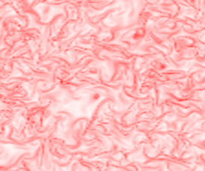
Here FTLE values based on the maximum eigenvalue from figure 2(b) are compared with FTLE values of the middle and smallest eigenvalue; see figure 17. As expected, the FTLE field of the middle one has both signs and is smaller in magnitude (see legend) than the other two. Also, the larger bright regions (LAMS) occur in all three images at the same locations.
The FTLE fields in a wall-parallel plane at  $\overline {y^+}=315$ of (a–c) the FTLE computed from the maximum, middle and smallest eigenvalue, respectively.

If the analysis is done with the forward-integrated FTLE field rather than the FTLE field calculated by backward integration, the data in figure 18(b) are obtained. The dark structures shown in figure 18(a) should be interpreted as accumulating the material in them (attracting LCS). With forward integration in figure 18(b), the dark structures represent the contrary effect, i.e. the material moves away from them (repelling LCS). It should be noted that the regions of minimal change occur in almost the same locations here compared with figure 18(a). Small differences are due to the fact that in the case of backward integration, time steps were used that lie before the one shown, and in the case of forward integration, later ones. So the integration is done over different time steps of the simulation leading to slightly different structures.
The FTLE fields in a wall-parallel plane at  $\overline {y^+}=315$ of (a) the FTLE computed by backward integration, (b) the FTLE computed by forward integration.


 Open access

