1 Introduction
Surface tension enables liquids to minimize their surface area, and to form various morphologies under external forces or geometrical constraints, such as puddles (de Gennes, Brochard-Wyart & Quéré Reference de Gennes, Brochard-Wyart and Quéré2003), thin/thick films (Debrégeas, De Gennes & Brochard-Wyart Reference Debrégeas, De Gennes and Brochard-Wyart1998; Craster & Matar Reference Craster and Matar2009), liquid rings (Texier et al. Reference Texier, Piroird, Quéré and Clanet2013), liquid layers with holes (Taylor & Michael Reference Taylor and Michael1973; Moriarty & Schwartz Reference Moriarty and Schwartz1993; López, Miksis & Bankoff Reference López, Miksis and Bankoff2001; Bankoff et al. Reference Bankoff, Johnson, Miksis, Schluter and Lopez2003; Dijksman et al. Reference Dijksman, Mukhopadhyay, Gaebler, Witelski and Behringer2015; Bostwick, Dijksman & Shearer Reference Bostwick, Dijksman and Shearer2017; Zheng et al. Reference Zheng, Fontelos, Shin, Dallaston, Tseluiko, Kalliadasis and Stone2018a ,Reference Zheng, Fontelos, Shin and Stone b ) or fingers (Craster & Matar Reference Craster and Matar2009), etc. Among them, a fundamental understanding of the statics and dynamics of liquid layers with holes is of crucial importance for numerous applications ranging from coating processes to micropatterning, because the aim of most processes is to produce a uniform film on a solid. A hole in a liquid layer is a defect that may grow or shrink, depending on the thickness of the layer, the wettability of the substrate as well as forces and constraints applied to the system.
The problem of growth and collapse of a dry spot in a thin liquid film is a classic example. Equilibrium solutions for the profiles of axisymmetric systems date back to the early comprehensive works of Lamb (Reference Lamb1916) and Padday (Reference Padday1971). Padday (Reference Padday1971) performed one of the first experimental studies of the process of forming and rupturing of a thin liquid film at a low-energy solid surface (wax or polytetrafluoroethylene), in which it was found that the liquid film ruptures when its thickness is smaller than a critical value. This critical thickness increases with the contact angle. A pioneering work carried out by Taylor & Michael (Reference Taylor and Michael1973) utilizing air jets to study hole formation in water and mercury films indicates the existence of a critical hole diameter representing the stability limit of an infinitely extended film with arbitrary thickness and arbitrary contact angle on the substrate. Experiments by the same authors on holes in a water layer on paraffin wax surface did not give an unambiguous picture of hole stability, but demonstrated a wide range of possibilities under which a hole can remain stationary (resulting from contact angle hysteresis). Moreover, only hydrophobic surfaces were considered.
Sparked by these seminal works, numerous studies have been devoted to the stability of a hole in a liquid layer. Using energy criteria, Sharma & Ruckenstein (Reference Sharma and Ruckenstein1990) theoretically showed that for a given contact angle in a finite domain, two isochoric holes of different radii are feasible. Their static analyses imply that any hole larger than a critical value will open up, otherwise it will close. The practically most relevant scenario involves liquid films whose thickness is dictated by a balance of gravitational and surface tension forces. It is known that holes in such capillary-stabilized liquid films are sensitive to the lateral extension of the film. Lubrication theory is commonly employed to compute the hole closure dynamics for finite liquid domains. Using a lubrication model, Moriarty & Schwartz (Reference Moriarty and Schwartz1993) studied the stability and evolution of an axisymmetric dry spot in a thin liquid film bounded by a rigid vertical wall, showing that the holes either close to form a uniform liquid film or open up until the stable equilibrium position is attained. Moreover, the contact line motion at the edge of the dry spot was taken into account and the contact line was moved artificially in their numerical solution, showing that a statically stable hole can be dynamically unstable if there is significant contact angle hysteresis. When the radius of the hole is small, axisymmetric equilibrium holes in thin liquid layers in an unbounded domain under the influence of surface tension and gravity have been studied by Wilson & Duffy (Reference Wilson and Duffy1996) using an asymptotic analysis. By employing linear stability theory, López et al. (Reference López, Miksis and Bankoff2001) found that for a substrate of a fixed diameter the axisymmetric equilibrium solutions with dry spots are unstable to axisymmetric disturbances, whereas, as the size of the dry spot increases, the equilibrium solutions become unstable to non-axisymmetric disturbances. Using the lubrication approximation, Zheng et al. (Reference Zheng, Fontelos, Shin, Dallaston, Tseluiko, Kalliadasis and Stone2018a ,Reference Zheng, Fontelos, Shin and Stone b ) studied the surface-tension-driven levelling dynamics of a thin viscous film after the closure of an initial hole, and they obtained a self-similar solution describing the dynamics of the film profile. However, theses results for the hole closure dynamics and hole stability are only valid for small contact angles.
The hole collapse in liquid layers has also been studied experimentally. In the work of Diez, Gratton & Gratton (Reference Diez, Gratton and Gratton1992), a closing dry spot in an axisymmetric flow of a very viscous fluid toward a central outlet was studied. The experiments were done in a region where there was a balance between gravity and viscous forces, whereas the surface tension effects were assumed to be small. A self-similar solution was constructed and shown to compare well with the experimental results after the radius of the dry spot is sufficiently small compared to its initial radius. By employing external forcing such as blowing, Bankoff et al. (Reference Bankoff, Johnson, Miksis, Schluter and Lopez2003) studied the diameter, front velocity, dynamic contact angle and interface shape related to a dry spot moving in a thin viscous film and their dependence on the film thickness. Their results show that the final size of the hole increases as the initial fluid depth decreases. Utilizing the centrifugal force by rotating an axisymmetric fluid reservoir, Dijksman et al. (Reference Dijksman, Mukhopadhyay, Gaebler, Witelski and Behringer2015) studied the hole collapse in a liquid film, ranging from the limit of pure gravitational driving to entirely surface-tension-driven flows. Very recently, Bostwick et al. (Reference Bostwick, Dijksman and Shearer2017) studied the collapse dynamics of an axisymmetric thin film that completely wets the bottom of a rotating container with vertical side walls. The effects of capillary, gravitational and centrifugal forces on this converging flow was analysed using lubrication theory. They report power-law forms for the collapse time when gravitational or surface tension forces dominate the dynamics. By a combination of theory and experimental work, Zheng et al. (Reference Zheng, Fontelos, Shin, Dallaston, Tseluiko, Kalliadasis and Stone2018a ) showed the existence of a self-similar solution for the profile and front location in the inward spreading process of a thin viscous liquid film filling a hole.
In spite of all these efforts, the dependence of the critical diameter and the collapse of a hole on the contact angle and the size of the liquid domain has remained largely obscure, partially because studying large contact angles goes beyond the commonly used lubrication theory. To gain further insights into the stability behaviour, we have established a set-up covering a broad range of parameters such as the contact angle and the extension of the liquid film.
In particular, the dynamics of the hole collapse is a prime example of a hydrodynamic singularity, and the time evolution of the collapse is found to follow a power law. However, the relative importance of the different driving forces (e.g. capillary force and gravitational force) and the relative importance of the different resistive forces (inertial and viscosity), as well as the geometry of the system, can alter the exponent in the power law. Redon, Brochard-Wyart & Rondelez (Reference Redon, Brochard-Wyart and Rondelez1991) found that the shrinking rate of the diameter
 $d$
of a dry patch obeys
 $d\sim t$
, which reflects the competition between capillary and viscous forces.
 $\text{d}d/\text{d}t$
is independent of
 $d$
or the film thickness, but inversely proportional to the viscosity and very sensitive to the contact angle. In the experiment of Diez et al. (Reference Diez, Gratton and Gratton1992), a highly viscous liquid was filled into the annular region in a circular basin limited by a concentric circular dam. When the dam is quickly lifted, a dry spot is created, and subsequently the surrounding liquid flows toward the centre. The diameter
 $d$
of the dry spot was found to scale
 $d\sim t^{0.762}$
. Dijksman et al. (Reference Dijksman, Mukhopadhyay, Gaebler, Witelski and Behringer2015) created a hole in a liquid layer in a rotating container. After stopping the rotation, a scaling law
 $d\sim t^{0.55}$
of the collapsing hole was found. The authors explained that the difference between their results and the results by Diez et al. (Reference Diez, Gratton and Gratton1992) is due to a larger influence of surface tension. Very recently, Bostwick et al. (Reference Bostwick, Dijksman and Shearer2017) theoretically studied the evolution of a collapsing hole in the lubrication approximation. For small Bond numbers, they obtained
 $d\sim t^{0.55}$
, whereas
 $d\sim t^{0.762}$
is the limiting behaviour for large Bond numbers. Very recently, Zheng et al. (Reference Zheng, Fontelos, Shin, Dallaston, Tseluiko, Kalliadasis and Stone2018a
) studied the healing of a perfectly wetting fluid film in a circular container. They found a
 $d\sim t^{0.49}$
scaling and demonstrated agreement between theory and experiments.
In this paper, we aim at a comprehensive understanding of the stability and collapse of a hole in a bounded liquid layer under the influence of gravity. The experiments were carried out by smoothly adding liquid to a film containing a hole until an unstable state is reached. In combination with a theoretical analysis, we clarify the influences resulting from the thickness and lateral extension of the liquid layer, as well as of the wettability of the substrate. Scaling laws describing the final stages of the collapse are identified, and the corresponding scaling coefficients are determined. It is recognized that the hole collapse is triggered by surface tension, after which the shrinking of the hole is predominantly driven by inertia, whereas the evolution of the liquid column after hole closure results from the balance between the capillary force and inertia. Our aim is to quantify the stability limit as well as the dynamics developing beyond stability and to explore the underlying physics. Shedding light on this problem will be relevant for a large number of industrial applications.
The paper is arranged as follows: in §§ 2 and 3, our focus lies on a static analysis. In § 2, we first present results from experiments including the initially quasi-static shrinkage of the hole, the onset of the instability when the hole diameter approaches a critical value and the influence of the wetting angle. In § 3, by employing different modelling and simulation approaches, we theoretically determine the critical diameter of the hole. We also demonstrate the independence of the critical hole diameter of the shape the surface bounding the liquid layer. The theoretical results are in good agreement with the experimental data. In § 4, we particularly focus on the dynamic evolution of the liquid surface after the instability has occurred. We analyse the pinch-off dynamics of the enclosed air bubble and determine the corresponding scaling laws. The paper is concluded in § 5.
2 Experimental analysis of hole stability
2.1 Experimental set-up and procedure
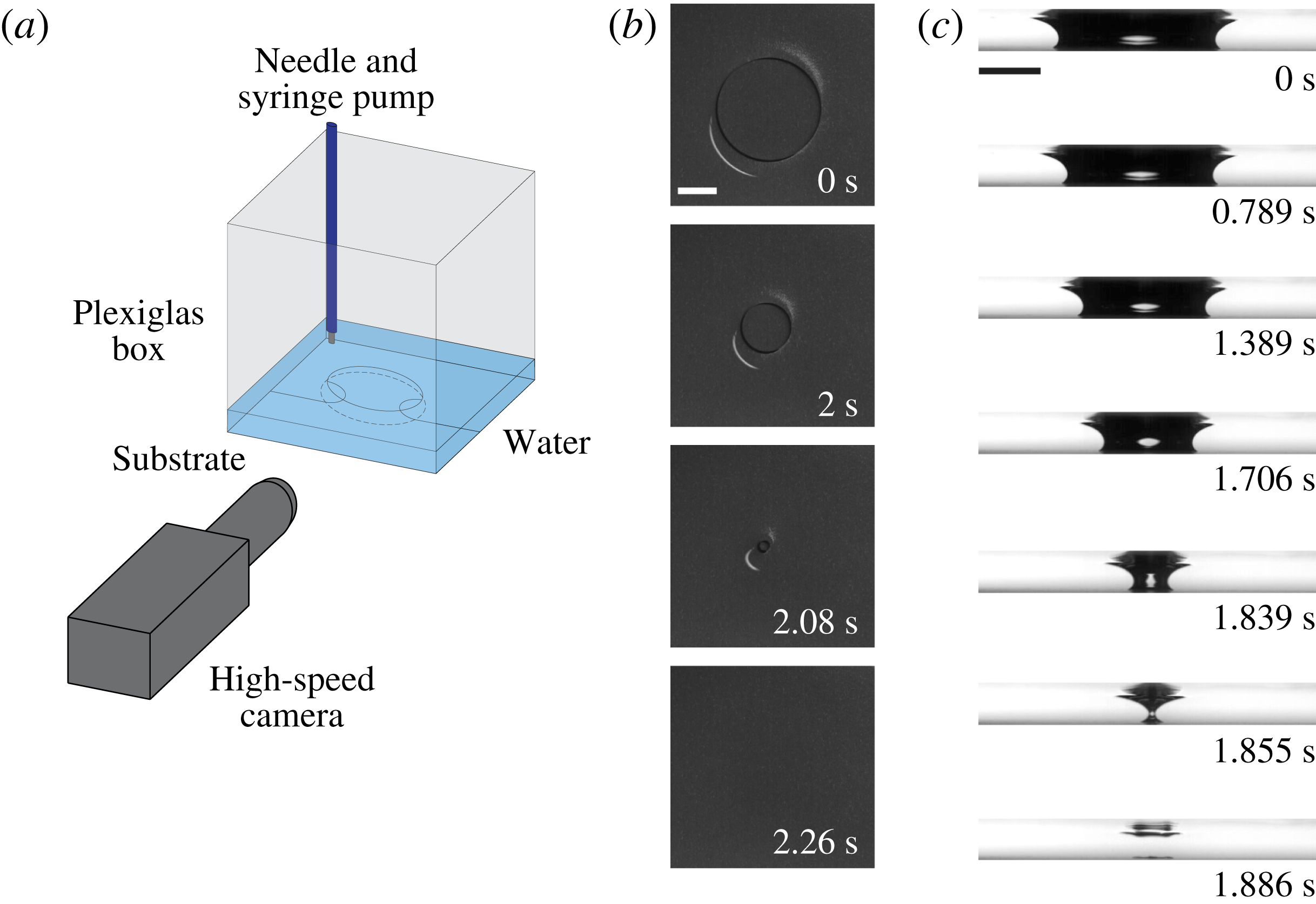
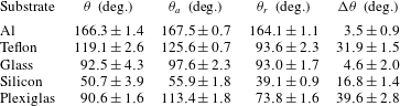
Our experimental set-up consists of a linear three-axis translation stage placed on an optical table, exchangeable flat substrates in Plexiglas boxes, a high-speed camera (Photron Fastcam SA1.1 Model 675K-M1) and a syringe pump (KD Scientific KDS 210 CE). To better visualize the liquid surface, boxes with square cross-section were employed. The box contains a layer of Milli-Q water, having a contact angle of close to
 $90^{\circ }$
with the Plexiglas walls (see table 1). A sketch of the set-up is displayed in figure 1(a).
(a) Schematic illustration of the experimental set-up with a needle connected to a syringe pump controlling the flow rate. Time lapse images of the collapse of a hole at the centre of a liquid layer on a bounded superhydrophobic Al plate are shown in top (b) and side (c) view, which are results from two different experiments. The top view indicates that the hole collapses with a circular shape. The side view (the dark regions are air and the light regions are water) suggests that the thickness of the liquid layer does not change appreciably relative to the situation before the collapse of the hole. The scale bars represent 10 mm.

We first carried out experiments using etched and silanized aluminium (Al) plates (Song et al.
Reference Song, Xu, Liu, Lu and Sun2012) to obtain a stable superhydrophobicity. On this surface, the advancing contact angle for water is
 $\unicode[STIX]{x1D703}_{a}=167.5^{\circ }\pm 0.7^{\circ }$
with a contact angle hysteresis of
 $\unicode[STIX]{x0394}\unicode[STIX]{x1D703}=3.5^{\circ }\pm 0.9^{\circ }$
, which guarantees a small contact line friction. In an experiment, we fix the Al plate at the bottom of the box and add a thin layer of water with an initial height
 ${\sim}h_{\infty }/2$
, after which we create a comparatively large hole at the centre of the substrate employing clean compressed air flow through a nozzle having an inner diameter of 3 mm. Here,
 $h_{\infty }=2l_{c}\sin (\unicode[STIX]{x1D703}/2)$
is the thickness of an infinite unbounded liquid layer (de Gennes et al.
Reference de Gennes, Brochard-Wyart and Quéré2003),
 $l_{c}\approx 2.73$
mm is the capillary length of water and
 $\unicode[STIX]{x1D703}$
is the contact angle on the substrate. The outlet of the nozzle is typically
 ${\sim}2$
cm away from the substrate and faces its central spot. When the hole has been created and reaches a circular shape, we stop the air flow. Shortly after that, the liquid film with the hole becomes static. Subsequently, using the syringe pump, we smoothly (flow rate
 $Q=0.1~\text{ml}~\text{min}^{-1}$
) add more water without any appreciable perturbation to the liquid layer. Six different boxes with a side length
 $L$
ranging from 7 cm to 19.5 cm were used. In the smallest box (
 $L=7$
cm), the height of the liquid layer only increases by
 $Q/L^{2}\approx 20.4~\unicode[STIX]{x03BC}\text{m}~\text{min}^{-1}$
(or
 ${\approx}0.3~\unicode[STIX]{x03BC}\text{m}~\text{s}^{-1}$
), which suggests that the liquid layer is very close to its static configuration while liquid is supplied. Therefore, the influence of the flow rate on the liquid layer is negligible.
2.2 Experimental observations
The time evolution of the hole is shown in figure 1(b,c) in top and side view, respectively.
 $t=0$
s is defined as the moment when the recording starts. During the experiments, imaging is typically performed with 500 frames per second (f.p.s.) to guarantee a long-time recording. In the regime of high-speed processes, i.e. after the collapse sets in, 73 000 f.p.s. are usually applied, but with a smaller field of view (fov). First, we observe that the size of the hole decreases smoothly maintaining a circular shape. In this state, if we stop adding water, the hole remains open and static. However, when the hole diameter
 $d$
reaches a specific value
 $d_{c}$
, the hole suddenly collapses (see supplementary movie 1 available at https://doi.org/10.1017/jfm.2018.680). This scenario is very different from the one studied by Taylor & Michael (Reference Taylor and Michael1973) or Bankoff et al. (Reference Bankoff, Johnson, Miksis, Schluter and Lopez2003), in which the authors first produced a liquid layer with a specific thickness, and then created a hole by removing an object which was placed in advance at the centre of the liquid layer or by blowing air using a capillary tube.
Before we go over to study the closure of the liquid film in more detail, it will be useful to provide an intuitive understanding of the key factors the hole collapse depends on. There are two principal curvatures of the liquid surface. The meridional curvature (see the cross-section in figure 1 c) creates a pressure jump favouring the opening of the hole. However, the azimuthal curvature or ‘hoop curvature’ (see the top view in figure 1 b) and the hydrostatic pressure push the liquid to the centre. The side views in figure 1(c) show that the liquid surface profiles are similar to each other at different instances, which indicates that the variations of the meridional curvature and the hydrostatic pressure are not pronounced. Therefore, the collapse of the liquid layer is caused by the pronounced increase of the hoop curvature as additional liquid is supplied.
As can be seen in side view (figure 1
c, see supplementary movie 2), when the hole closes, the remaining air is divided into two parts, i.e. an air bubble remains at the surface (
 $t=1.855$
s). Subsequently, the air bubble is compressed to a pancake shape, which is very similar to the spreading of air bubbles on superhydrophobic substrates reported very recently (de Maleprade, Clanet & Quéré Reference de Maleprade, Clanet and Quéré2016). In the following, the air bubble disappears. However, in experiments carried out on other substrates (e.g. Teflon, see supplementary movie 3) the air bubble remains, which indicates that on the Al surface the air goes to the micro- and nanoscopic cavities and might be dissolved. Finally, the liquid film at the coalescence point grows, and the whole liquid layer reaches a uniform thickness. The thickness after hole collapse is not significantly different from the thickness before the onset of the collapse.
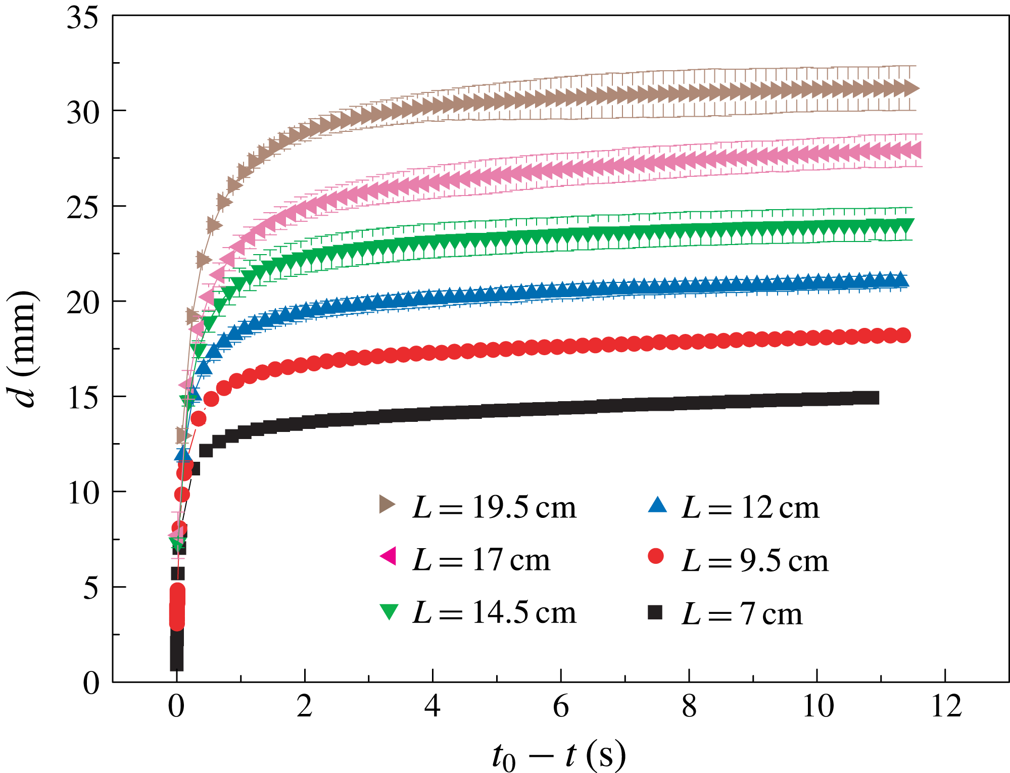
Time evolution of holes in liquid layers. The plot shows the instantaneous diameter
 $d$
of the hole as a function of time
 $(t_{0}-t)$
on superhydrophobic Al surfaces.
 $t_{0}$
is defined as the moment when
 $d=0$
. All the data points are average values of five experiments with error bars representing the standard deviation. Six boxes with a side length
 $L$
ranging from 7 cm to 19.5 cm have been employed.

In order to quantify the dynamics of the hole, we plot the relationship between the instantaneous value of
 $d$
and time
 $(t_{0}-t)$
for a large range of box sizes, denoting
 $t_{0}$
the moment when
 $d=0$
, as shown in figure 2. The instantaneous diameter
 $d$
of the hole is determined as the minimum value of the neck of the air phase (the dark regions visible in figure 1
c). The data points in the relationship between
 $d$
and
 $(t_{0}-t)$
were obtained by averaging five experiments, with corresponding error bars. Figure 2 clearly demonstrates the existence of two regimes, namely a region with a small slope and a region with a higher slope. In the former regime, since the hole remains open with a specific static diameter
 $d$
when the feeding is stopped, the shrinking is caused by the flow due to the pump. We refer to this situation as the hole being stable. On the contrary, in the latter regime the hole starts to close even as the feeding is stopped, so the hole is unstable. The methods employed in most of the previous research only capture the latter regime, for example by removing a barrier in the central region of the liquid film (e.g. Taylor & Michael Reference Taylor and Michael1973; Diez et al.
Reference Diez, Gratton and Gratton1992; Bankoff et al.
Reference Bankoff, Johnson, Miksis, Schluter and Lopez2003; Zheng et al.
Reference Zheng, Fontelos, Shin, Dallaston, Tseluiko, Kalliadasis and Stone2018a
,Reference Zheng, Fontelos, Shin and Stone
b
).
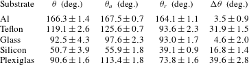
The universality of the above results was checked through experiments with substrates of different wettabilities. Apart from the superhydrophobic Al plates, three other substrates, namely liquid infused glass (
 $\unicode[STIX]{x1D703}_{a}=97.6\pm 2.3^{\circ }$
,
 $\unicode[STIX]{x0394}\unicode[STIX]{x1D703}=4.6\pm 2.0^{\circ }$
) (Eifert et al.
Reference Eifert, Paulssen, Varanakkottu, Baier and Hardt2014) Teflon (
 $\unicode[STIX]{x1D703}_{a}=125.6\pm 0.7^{\circ }$
,
 $\unicode[STIX]{x0394}\unicode[STIX]{x1D703}=31.9\pm 1.5^{\circ }$
) and silicon (
 $\unicode[STIX]{x1D703}_{a}=55.9\pm 1.8^{\circ }$
,
 $\unicode[STIX]{x0394}\unicode[STIX]{x1D703}=16.8\pm 1.4^{\circ }$
), were employed (see table 1). For this purpose, all experiments were performed in the same square box (
 $L=7$
cm). For the liquid-infused glass and Teflon surfaces, the diameter
 $d$
as the function of time
 $t$
shows a similar behaviour as in figure 2. As already indicated, after the closure of the hole, an air bubble remains on the Teflon (see supplementary movie 3) and glass substrates.
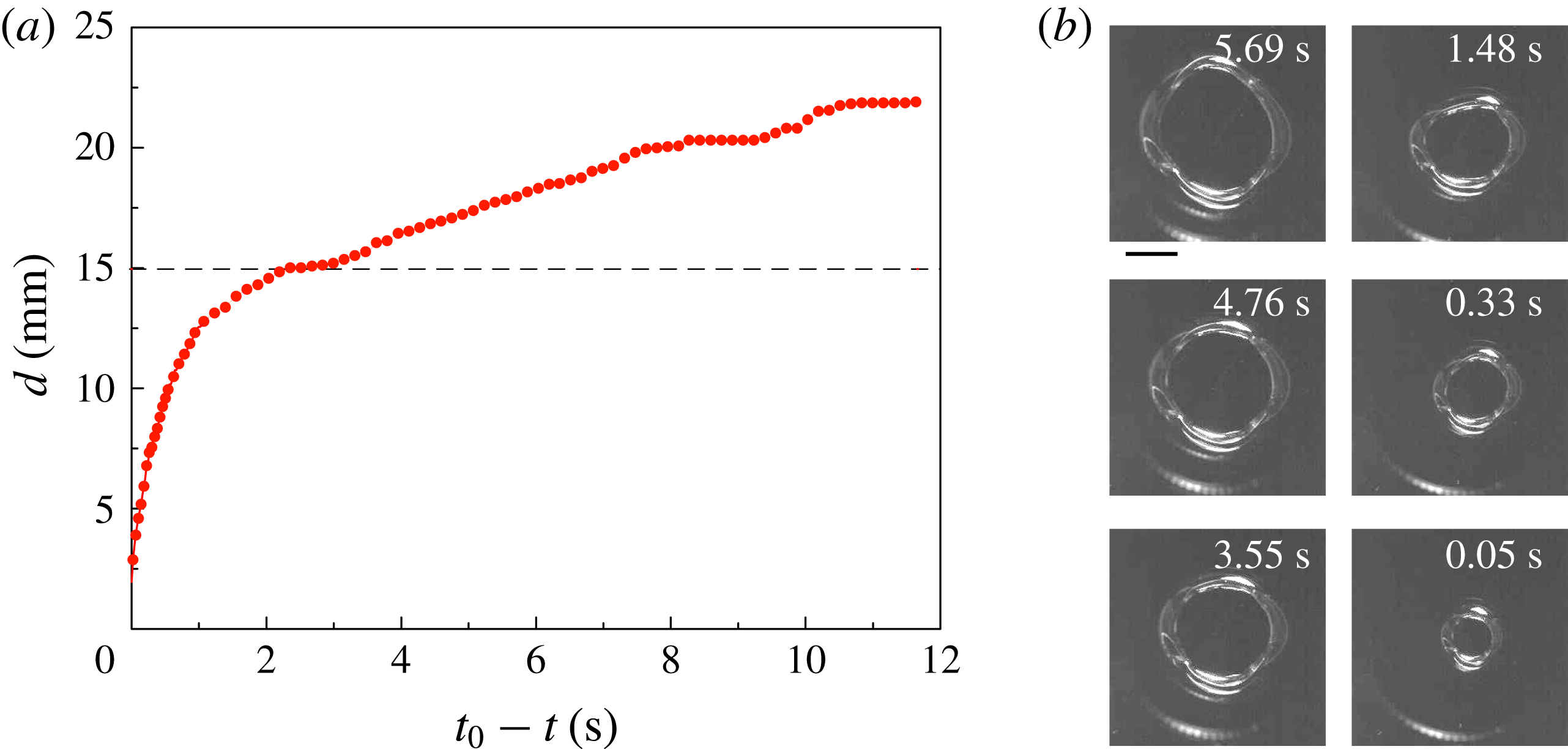
Evolution of
 $d$
with time
 $(t_{0}-t)$
on a silicon substrate in a square box of
 $L=7$
cm. (a) The red dots are experimental results, and the dashed line is the prediction for
 $d_{c}$
based on the asymptotic analytical solution (see § 3.2). (b) Selected frames from another experiment in top view. The scale bar represents 10 mm. The brightness (in sharp contrast to the other parts) around the three-phase contact line results from the reflection of the light source.

Particularly, we would like to take a more detailed look at the hole on the silicon wafer (see supplementary movie 4). The experimental procedure is the same as described in § 2.1. In figure 3(a),
 $d$
is plotted as a function of (
 $t_{0}-t$
) for the
 $L=7$
cm box. Owing to the higher contact angle hysteresis (see table 1), the curve for the silicon wafer is not as smooth as for the Al surface (see figure 2). Before
 $d$
reaches
 $d_{c}$
, several pinning/depinning events occur (i.e.
 $(t_{0}-t)\in [2,4]$
s,
 $[8,10]$
s,
 $[12,14]$
s). However, after reaching
 $d_{c}$
(the dashed line in figure 3
a), a smoother dynamics is observed. Selected frames are displayed in figure 3(b), showing the hole shapes on the silicon substrate in top view, indicating that the solid–liquid–gas three-phase contact lines deviate from a circular shape. This is the reason for the larger error bars in the experiments on silicon wafers in comparison to the other substrates, as shown in figure 3(b). Surprisingly, even if the contact angle hysteresis on Teflon is higher than that on silicon, a smoother evolution of the contact line was observed on Teflon (see supplementary movie 3). So far, the reasons behind that are unclear.
3 Modelling the quasi-static behaviour
In order to understand the underlying mechanisms, we first compute the equilibrium shape of the liquid surface under the influence of surface tension and gravity. Since the influence of the flow rate on the evolution of the liquid layer is negligible, we propose the convenient simplification of reducing the problem to a succession of quasi-static liquid profiles.
Based on that, the profile of the liquid layer is controlled by the Young–Laplace equation,
 $$\begin{eqnarray}\unicode[STIX]{x0394}p=2\unicode[STIX]{x1D705}\unicode[STIX]{x1D6FE}=\unicode[STIX]{x0394}p_{0}+\unicode[STIX]{x1D70C}gz,\end{eqnarray}$$
where
 $\unicode[STIX]{x0394}p$
,
 $2\unicode[STIX]{x1D705}$
and
 $\unicode[STIX]{x1D6FE}$
are the Laplace pressure, the curvature of the liquid surface and the surface tension, respectively.
 $\unicode[STIX]{x1D70C}$
,
 $g$
and
 $z$
are the mass density of the liquid, the gravitational acceleration and the vertical coordinate.
 $\unicode[STIX]{x0394}p_{0}$
is the Laplace pressure at
 $z=0$
.
Since the known analytical solutions of the Young–Laplace equation including gravity are limited to specific cases (Norbury, Sander & Scott Reference Norbury, Sander and Scott2004), in § 3.1 we solve (3.1) numerically in an axisymmetric coordinate system. Correspondingly, the volume and potential energy of the liquid layer are obtained. That way, the liquid film can be studied on different substrates with arbitrary values of the contact angle. In addition, we derive an asymptotic model in § 3.2, which is valid for liquid layers with small contact angles to the substrate.
3.1 Numerical solution of the Young–Laplace equation
Considering that the contact angle between water and the box walls is close to
 $90^{\circ }$
, we assume on the one hand that the perturbation caused by the boundaries/edges of the box does not influence the shape of the liquid surface very much. On the other hand, we assume that the shape (square or circular) of the box does not affect the stability of the liquid layer. This assumption is verified in appendix B.
Including gravity, the Young–Laplace equation takes the following form in an axisymmetric coordinate system,
 $$\begin{eqnarray}\displaystyle & \displaystyle -\left(\frac{\text{d}\unicode[STIX]{x1D711}}{\text{d}s}+\frac{\sin \unicode[STIX]{x1D711}}{r}\right)\unicode[STIX]{x1D6FE}=\unicode[STIX]{x0394}p_{0}-\unicode[STIX]{x1D70C}gz, & \displaystyle\end{eqnarray}$$
 $$\begin{eqnarray}\displaystyle & \displaystyle \frac{\text{d}r}{\text{d}s}=\cos \unicode[STIX]{x1D711}, & \displaystyle\end{eqnarray}$$
 $$\begin{eqnarray}\displaystyle & \displaystyle \frac{\text{d}z}{\text{d}s}=\sin \unicode[STIX]{x1D711}, & \displaystyle\end{eqnarray}$$
where
 $s$
is the arc-length along the liquid surface, and
 $\unicode[STIX]{x1D711}$
is the tangential angle (i.e.
 $\unicode[STIX]{x1D711}=\arctan (\text{d}z/\text{d}r)$
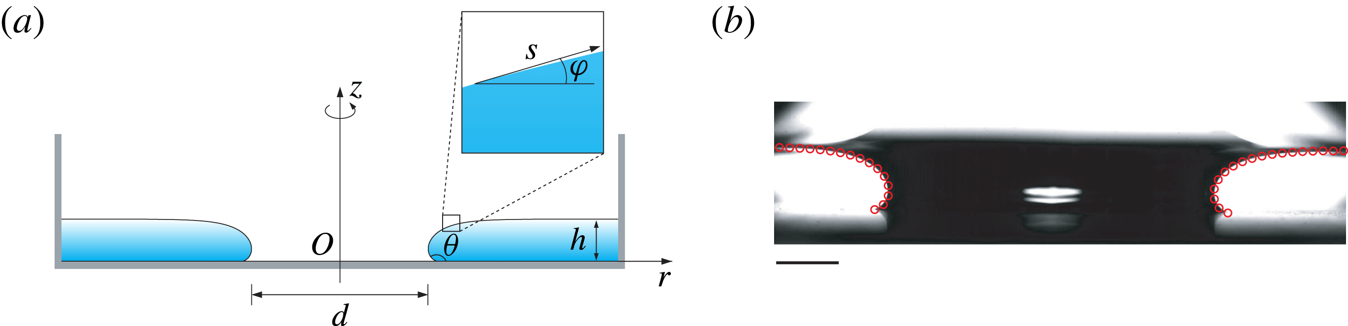
), as shown in figure 4(a). Here, we choose
 $s$
and
 $\unicode[STIX]{x1D711}$
as the only two variables parametrizing the surface. For convenience, by introducing the capillary length
 $l_{c}$
, we define dimensionless forms of the relevant geometrical and physical quantities,
 $$\begin{eqnarray}\tilde{r}=\frac{r}{l_{c}},\quad \tilde{z}=\frac{z}{l_{c}},\quad \tilde{s}=\frac{s}{l_{c}},\quad \unicode[STIX]{x0394}\tilde{p}=\frac{\unicode[STIX]{x0394}pl_{c}}{\unicode[STIX]{x1D6FE}},\end{eqnarray}$$
and we rewrite (3.2)–(3.4) into
 $$\begin{eqnarray}\displaystyle & \displaystyle -\left(\frac{\text{d}\unicode[STIX]{x1D711}}{\text{d}\tilde{s}}+\frac{\sin \unicode[STIX]{x1D711}}{\tilde{r}}\right)=\unicode[STIX]{x0394}\tilde{p}_{0}-\tilde{z}, & \displaystyle\end{eqnarray}$$
 $$\begin{eqnarray}\displaystyle & \displaystyle \frac{\text{d}\tilde{r}}{\text{d}\tilde{s}}=\cos \unicode[STIX]{x1D711}, & \displaystyle\end{eqnarray}$$
 $$\begin{eqnarray}\displaystyle & \displaystyle \frac{\text{d}\tilde{z}}{\text{d}\tilde{s}}=\sin \unicode[STIX]{x1D711}, & \displaystyle\end{eqnarray}$$
with three initial conditions
 $\unicode[STIX]{x1D711}|_{\tilde{s}=0}=\unicode[STIX]{x1D703}$
,
 $\tilde{r}|_{\tilde{s}=0}=\tilde{d}/2$
,
 $\tilde{z}|_{\tilde{s}=0}=0$
. To solve these three first-order ordinary nonlinear and coupled differential equations, a shooting method was employed. Our shooting method is based on changing the values of the two unknown parameters
 $\tilde{s}_{tot}$
and
 $\unicode[STIX]{x0394}\tilde{p}_{0}$
until the following two boundary conditions are satisfied,
 $$\begin{eqnarray}\tilde{V}|_{\tilde{s}=\tilde{s}_{tot}}=\tilde{V}_{0},\quad \unicode[STIX]{x1D711}|_{\tilde{s}=\tilde{s}_{tot}}=0,\end{eqnarray}$$
in which
 $V_{0}$
is the volume of the liquid for a specific configuration (which corresponds to a specific value of
 $d$
for a static state), and
 $s_{tot}$
is the total arc-length. The calculations were performed using the Matlab function ode45. Figure 4(b) demonstrates good agreement between the theory and the experimental results (more comparisons for various values of
 $\unicode[STIX]{x1D703}$
are shown in the supplementary material). After the solutions for the surface profile have been determined, other relevant geometrical and physical quantities such as the curvature at an arbitrary point and each contribution to the total energy of the system (i.e. surface energy and gravitational energy) can also be obtained.
(a) Axisymmetric liquid layer profile shown in side view,
 $d$
is the diameter of the hole and
 $s$
is the arc-length along the liquid surface. As shown in the inset, the tangential angle
 $\unicode[STIX]{x1D711}$
is defined as
 $\unicode[STIX]{x1D711}=\arctan (\text{d}z/\text{d}r)$
. (b) Comparison between the numerical results of § 3.1 (red hollow circles) and the experimental results. The substrate is the superhydrophobic Al plate with
 $\unicode[STIX]{x1D703}_{a}=167.5^{\circ }$
, the box size is
 $L=14.5$
cm and
 $d=26.1$
mm in the current frame. The scale bar represents 5 mm.

In figure 5, two cases are studied: (i) liquid layers on a completely non-wetting surface (i.e.
 $\unicode[STIX]{x1D703}=180^{\circ }$
) in six circular boxes with various diameters
 $L$
ranging from 7 cm to 19.5 cm, which is much larger than the capillary length
 $l_{c}$
; (ii) liquid layers in a (circular) box with diameter
 $L=14.5$
cm, but with varying contact angles ranging from
 $\unicode[STIX]{x1D703}=5^{\circ }$
to
 $\unicode[STIX]{x1D703}=180^{\circ }$
. The data in figure 5 are normalized by
 $l_{c}$
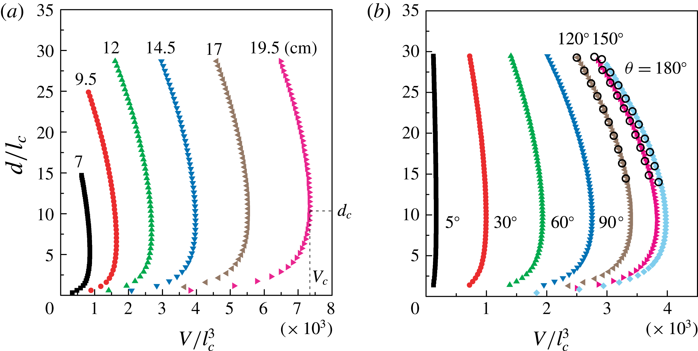
. For each curve, when the hole diameter is large, the liquid volume
 $V$
increases with decreasing
 $d$
. However, a maximum volume
 $V_{c}$
exists, corresponding to a critical value of
 $d_{c}$
. Based on the minimum-volume theorem formulated in Langbein (Reference Langbein2002), the point (
 $V_{c},d_{c}$
) corresponds to a point of instability. Up to now, the critical diameter has only been obtained based on a small contact angle approximation (Moriarty & Schwartz Reference Moriarty and Schwartz1993). If
 $d<d_{c}$
, solutions of (3.1) exist mathematically, but they are unstable (Moriarty & Schwartz Reference Moriarty and Schwartz1993) and do not correspond to any physically observable configuration. In our experiments, the volume of the liquid film is increased monotonously until it reaches the maximum
 $V_{c}$
. Since the syringe pump is always running, the liquid volume finally exceeds
 $V_{c}$
, reaching a regime where no stable solution of the Young–Laplace equation exists, so the hole collapses. Furthermore, our results indicate the existence of a finite value of
 $d_{c}$
, no matter what the size of the box or the contact angle on the substrate is. If we increase the box size beyond all limits, our results converge to the results obtained by Taylor & Michael (Reference Taylor and Michael1973) with
 $h=2l_{c}\sin (\unicode[STIX]{x1D703}/2)$
, suggesting a stable infinite hole diameter (see figure 8 in Taylor & Michael Reference Taylor and Michael1973).
Numerical solutions of (3.1) showing the dependence of
 $V$
on
 $d$
when varying the size of the box and the wettability of the substrate. The data are normalized by the capillary length
 $l_{c}$
. (a) The contact angle is fixed, i.e.
 $\unicode[STIX]{x1D703}=180^{\circ }$
. Circular boxes with six different diameters
 $L$
are employed, i.e.
 $L=7.0$
cm, 9.5 cm, 12.0 cm, 14.5 cm, 17.0 cm, 19.5 cm.
 $V_{c}$
and
 $d_{c}$
denote the critical values of the volume and the hole diameter when the instability occurs. (b) The box diameter is fixed to
 $L=14.5$
cm, and contact angles of
 $\unicode[STIX]{x1D703}=5^{\circ }$
,
 $30^{\circ }$
,
 $60^{\circ }$
,
 $90^{\circ }$
,
 $120^{\circ }$
,
 $150^{\circ }$
,
 $180^{\circ }$
are considered. The black hollow circles are numerical solutions obtained by surface evolver using a square box with a side length of
 $L=14.5$
cm (see appendix B).

3.2 Asymptotic model for small contact angles
If the contact angle
 $\unicode[STIX]{x1D703}$
is very small
 $(\unicode[STIX]{x1D703}\ll 1)$
, on the basis of the following approximations,
 $$\begin{eqnarray}\sin \unicode[STIX]{x1D711}\approx \unicode[STIX]{x1D711}\approx \frac{\text{d}\tilde{z}}{\text{d}\tilde{r}},\quad \frac{\text{d}\unicode[STIX]{x1D711}}{\text{d}\tilde{s}}\approx \frac{\text{d}^{2}\tilde{z}}{\text{d}\tilde{r}^{2}}\end{eqnarray}$$
we can rewrite (3.6) into a linear second-order ordinary differential equation,
 $$\begin{eqnarray}\frac{\text{d}^{2}\tilde{z}}{\text{d}\tilde{r}^{2}}+\frac{1}{\tilde{r}}\frac{\text{d}\tilde{z}}{\text{d}\tilde{r}}-\tilde{z}=-\unicode[STIX]{x0394}\tilde{p}_{0}.\end{eqnarray}$$
Considering the boundary conditions
 $\tilde{z}|_{\tilde{r}=\tilde{d}/2}=0$
,
 $\tilde{z}^{\prime }|_{\tilde{r}=\tilde{d}/2}=\tan \unicode[STIX]{x1D703}$
,
 $\tilde{z}^{\prime }|_{\tilde{r}=\tilde{L}/2}=0$
(
 $\unicode[STIX]{x0394}\tilde{p}_{0}$
is a Lagrange multiplier, which can be obtained using the boundary conditions), an analytical solution of the above equation can be obtained,
 $$\begin{eqnarray}\tilde{z}(\tilde{r})=\frac{\text{I}_{1}\left({\displaystyle \frac{\tilde{L}}{2}}\right)\left[\text{K}_{0}(\tilde{r})-\text{K}_{0}\left({\displaystyle \frac{\tilde{d}}{2}}\right)\right]+\text{K}_{1}\left({\displaystyle \frac{\tilde{L}}{2}}\right)\left[\text{I}_{0}(\tilde{r})-\text{I}_{0}\left({\displaystyle \frac{\tilde{d}}{2}}\right)\right]}{\text{I}_{1}\left({\displaystyle \frac{\tilde{d}}{2}}\right)\text{K}_{1}\left({\displaystyle \frac{\tilde{L}}{2}}\right)-\text{I}_{1}\left({\displaystyle \frac{\tilde{L}}{2}}\right)\text{K}_{1}\left({\displaystyle \frac{\tilde{d}}{2}}\right)}\tan \unicode[STIX]{x1D703},\end{eqnarray}$$
where
 $\text{I}_{n}$
is the modified Bessel function of the first kind and
 $\text{K}_{n}$
is the Bessel function of the second kind (Magnus, Oberhettinger & Soni Reference Magnus, Oberhettinger and Soni1966). Note that this solution has already been obtained by Moriarty & Schwartz (Reference Moriarty and Schwartz1993) and used by López et al. (Reference López, Miksis and Bankoff2001). It further leads to an analytical solution for the volume
 $V$
 $$\begin{eqnarray}\tilde{V}\left(\frac{\tilde{d}}{2}\right)=(\unicode[STIX]{x1D6E4}_{1}+\unicode[STIX]{x1D6E4}_{2})\unicode[STIX]{x03C0}\tan \unicode[STIX]{x1D703},\end{eqnarray}$$
with
 $$\begin{eqnarray}\displaystyle & \displaystyle \unicode[STIX]{x1D6E4}_{1}=\frac{\left[{\displaystyle \frac{1}{4}}(\tilde{d}^{2}-\tilde{L}^{2})\text{I}_{0}\left({\displaystyle \frac{\tilde{d}}{2}}\right)-\tilde{d}\text{I}_{1}\left({\displaystyle \frac{\tilde{d}}{2}}\right)\right]\text{K}_{1}\left({\displaystyle \frac{\tilde{L}}{2}}\right)}{\text{I}_{1}\left({\displaystyle \frac{\tilde{d}}{2}}\right)\text{K}_{1}\left({\displaystyle \frac{\tilde{L}}{2}}\right)-\text{I}_{1}\left({\displaystyle \frac{\tilde{L}}{2}}\right)\text{K}_{1}\left({\displaystyle \frac{\tilde{d}}{2}}\right)}, & \displaystyle\end{eqnarray}$$
 $$\begin{eqnarray}\displaystyle & \displaystyle \unicode[STIX]{x1D6E4}_{2}=\frac{\left[{\displaystyle \frac{1}{4}}(\tilde{d}^{2}-\tilde{L}^{2})\text{K}_{0}\left({\displaystyle \frac{\tilde{d}}{2}}\right)+\tilde{d}\text{K}_{1}\left({\displaystyle \frac{\tilde{d}}{2}}\right)\right]\text{I}_{1}\left({\displaystyle \frac{\tilde{L}}{2}}\right)}{\text{I}_{1}\left({\displaystyle \frac{\tilde{d}}{2}}\right)\text{K}_{1}\left({\displaystyle \frac{\tilde{L}}{2}}\right)-\text{I}_{1}\left({\displaystyle \frac{\tilde{L}}{2}}\right)\text{K}_{1}\left({\displaystyle \frac{\tilde{d}}{2}}\right)}. & \displaystyle\end{eqnarray}$$
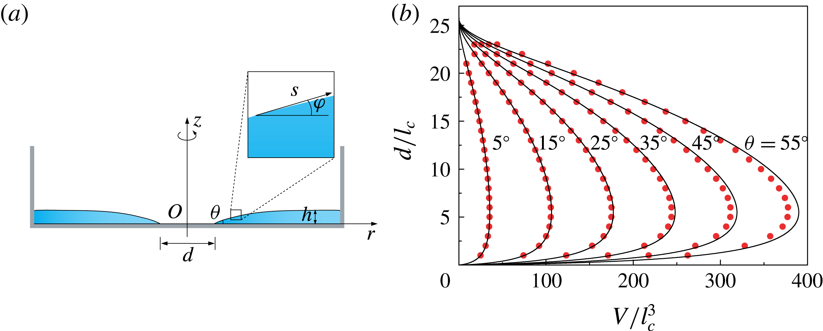
To test the quality of the small-angle approximation the analytical solution is based on, we choose
 $L=7$
cm. Figure 6(b) shows a series of analytical results for
 $d$
versus
 $V$
(solid lines) together with the numerical solutions (red dots) for different contact angles. It becomes clear that the asymptotic solution is still accurate for contact angles up to
 $\unicode[STIX]{x1D703}\approx 35^{\circ }$
.
(a) Axisymmetric liquid profile shown in side view (
 $\unicode[STIX]{x1D703}\ll 1$
). The geometrical parameters are the same as those defined in figure 4(a). (b) Dependence of the diameter
 $d$
on the volume
 $V$
in dimensionless form for different contact angles in a circular box with
 $L=7$
cm. The black solid lines represent the asymptotic theory, and the red dots are numerical results obtained as described in § 3.1.

To find the critical diameter
 $d_{c}$
, we have to determine the maximum value of the function given in (3.13) by solving
 $\text{d}V/\text{d}d=0$
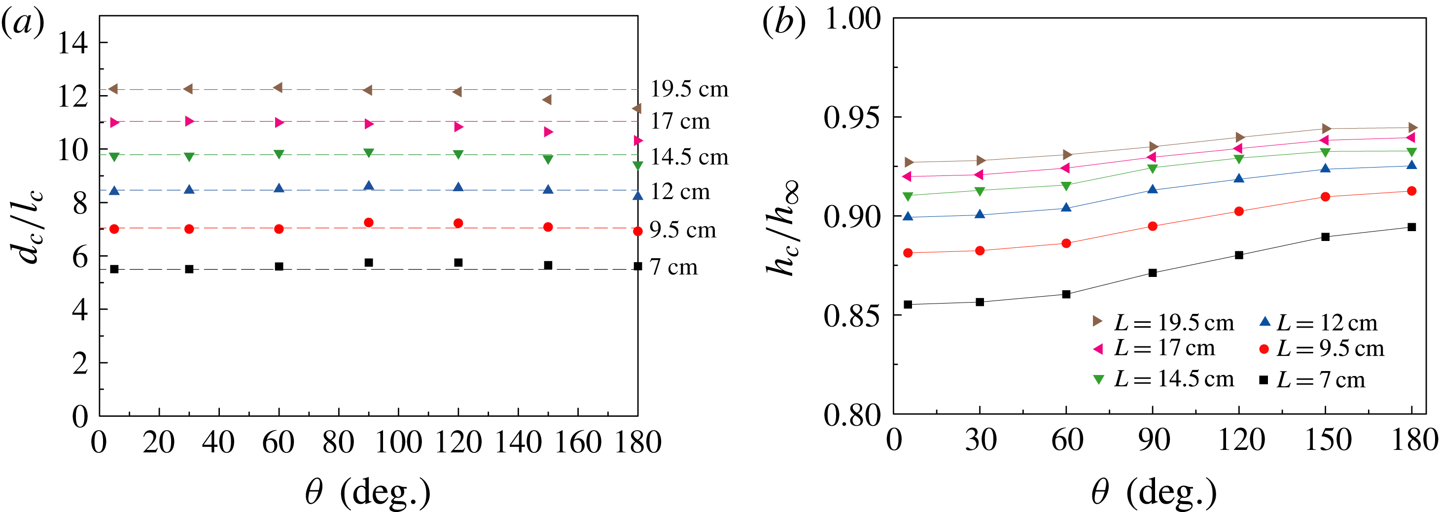
, which has been done numerically. In figure 7(a), we show the dependency of
 $d_{c}$
on
 $\unicode[STIX]{x1D703}$
in dimensionless form for box sizes ranging from 7 to 19.5 cm (which correspond to the values chosen in our experiments). The dashed lines are the values of
 $d_{c}$
obtained from the asymptotic solution, and the dots are the numerical results obtained in § 3.1.
Figure 7(a) suggests a weak contact angle dependence of
 $d_{c}$
but a stronger dependence on the size of the box. First we focus on the case when
 $\unicode[STIX]{x1D703}$
is small. In this regime the asymptotic model given in the above follows the numerical results (figures 6
b, 7
a) very well. Based on figures 5 and 6(b), we know that
 $d_{c}$
is determined from
 $\text{d}V/\text{d}d=0$
. From (3.13) we can see that
 $\text{d}V/\text{d}d=0$
corresponds to
 $\text{d}(\unicode[STIX]{x1D6E4}_{1}+\unicode[STIX]{x1D6E4}_{2})/\text{d}d=0$
, because
 $\unicode[STIX]{x1D703}$
is a material parameter but not a function of
 $d$
or
 $L$
. Equations (3.14) and (3.15) tell us that
 $\unicode[STIX]{x1D6E4}_{1}$
and
 $\unicode[STIX]{x1D6E4}_{2}$
are just functions of
 $d$
and
 $L$
. In other words, if
 $L$
is given,
 $d_{c}$
can be uniquely determined and does not depend on the contact angle
 $\unicode[STIX]{x1D703}$
. This is the reason why in figure 7(a), when
 $L$
is given,
 $d_{c}$
does not depend on
 $\unicode[STIX]{x1D703}$
. Furthermore,
 $d_{c}$
decreases for larger contact angles, which means that the asymptotic solution represents an upper limit for
 $d_{c}$
. Although the asymptotic result is obtained based on small contact angles, the comparison shows that it agrees well with the numerical results even for
 $\unicode[STIX]{x1D703}\approx 90^{\circ }$
. Secondly, by employing a simplified model in which it is assumed that the fluid film has a rectangular cross-section (see the supplementary material), the slight decrease of
 $d_{c}$
with
 $\unicode[STIX]{x1D703}$
and the dependence of
 $d_{c}$
on the size of the container are qualitatively explained.
Figure 7(b) shows the importance of considering finite box sizes. For a specific contact angle, the approach of
 $h_{c}/h_{\infty }$
towards 1 becomes slower and slower with increasing
 $L$
, where
 $h_{c}$
is the film thickness at the boundary of the box in the configuration where the critical hole diameter is reached. As one example, when
 $\unicode[STIX]{x1D703}=180^{\circ }$
and
 $L=19.5$
cm,
 $h_{c}/h_{\infty }\approx 0.9476$
. In other words, for obtaining values of
 $h_{c}$
very close to
 $h_{\infty }$
, the size of the box needs to be extremely large. Simultaneously,
 $d_{c}$
increases with increasing box size. In the limiting case, i.e.
 $L\rightarrow \infty$
, our results converge to the results obtained by Taylor & Michael (Reference Taylor and Michael1973) leading to an infinite critical diameter
 $d_{c}$
.
(a) Dependence of
 $d_{c}$
on
 $\unicode[STIX]{x1D703}$
for six different box sizes. The dashed lines represent the asymptotic result (
 $\unicode[STIX]{x1D703}\ll 1$
), and the symbols are numerical solutions obtained in § 3.1. (b) Numerical results for the critical height
 $h_{c}$
(corresponding to
 $d_{c}$
) scaled by
 $h_{\infty }$
as a function of the contact angle
 $\unicode[STIX]{x1D703}$
.
 $h_{c}$
is the film thickness at the boundary of the box.

3.3 Comparison between experimental results and model results
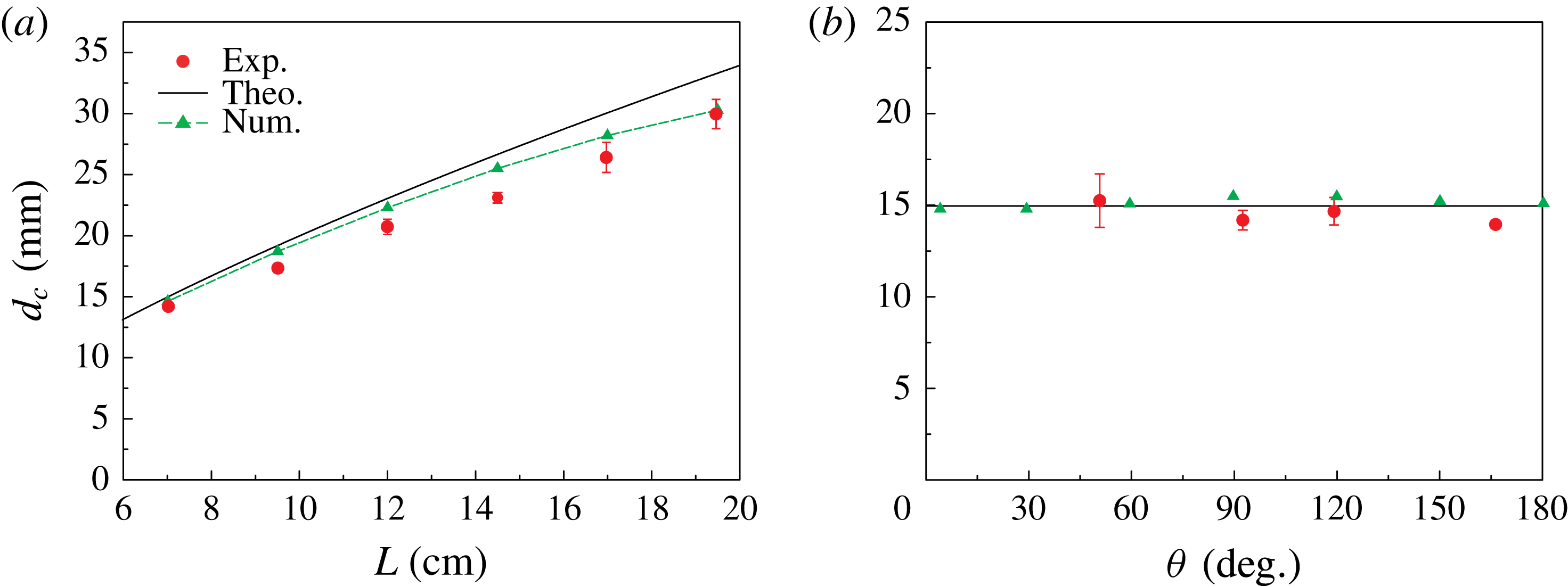
In figure 8(a), results obtained on superhydrophobic Al substrates in square boxes of different sizes are displayed. The red dots represent the experimental values of
 $d_{c}$
(see appendix C) that have been obtained as the average of five measurements. The green triangles are numerical results extracted from the data shown in figure 5(a) (i.e. the critical values
 $d_{c}$
and
 $V_{c}$
corresponding to the maximum volume). Even though the asymptotic model is constructed based on the assumption
 $\unicode[STIX]{x1D703}\ll 1$
and cannot be justified for large contact angles a priori, the numerical simulations suggest a weak dependence of
 $d_{c}$
on the contact angle. Therefore, we also show the results of the asymptotic theory, represented by the black solid line. Figure 8(a) shows that
 $d_{c}$
increases with
 $L$
. The experimental and the numerical results are consistent with each other. In spite of its inherent assumption of small contact angles, even the asymptotic method provides a reasonable approximation to the experimental data.
Figure 8(b) clearly shows that stable holes exist for a wide range of contact angles. Moreover,
 $d_{c}$
is virtually independent of the contact angle, and the experimental results are consistent with the numerical and theoretical results according to §§ 3.1 and 3.2.
(a) Dependence of
 $d_{c}$
on
 $L$
on superhydrophobic Al surfaces. The experiments were performed in square boxes with
 $L=7.0$
cm, 9.5 cm, 12.0 cm, 14.5 cm, 17.0 cm and 19.5 cm. The green triangles are numerical results (in circular boxes with different box diameters
 $L$
, see § 3.1) with the green dashed line as a guide for the eye. The black solid line is the theoretical result based on an asymptotic method for small contact angles (in circular boxes with different box diameters
 $L$
, see § 3.2). (b)
 $d_{c}$
as a function of the contact angle. Four different contact angles (red dots) have been studied experimentally in the square box with
 $L=7$
cm. The green triangles are numerical results. The black solid line is the asymptotic solution for
 $d_{c}$
. All the red dots are average values of five experiments with error bars representing the standard deviation.

4 Dynamic behaviour
When
 $d$
falls below
 $d_{c}$
, a highly dynamic process sets in, as shown in figures 1 and 2. In this section, we discuss the dynamics of hole collapse and the variation of the thickness of the liquid column after hole closure (see supplementary movie 5). To reveal the underlying mechanics during these processes, we also study the influence resulting from the viscosity. Scaling laws for the different processes are identified.
4.1 Dynamics of hole collapse
To better resolve the final moments of hole collapse, additional experiments were performed with a high time resolution when
 $t\rightarrow t_{0}$
. The complete time evolution of
 $d$
, starting from the initial moment when
 $d\gg d_{c}$
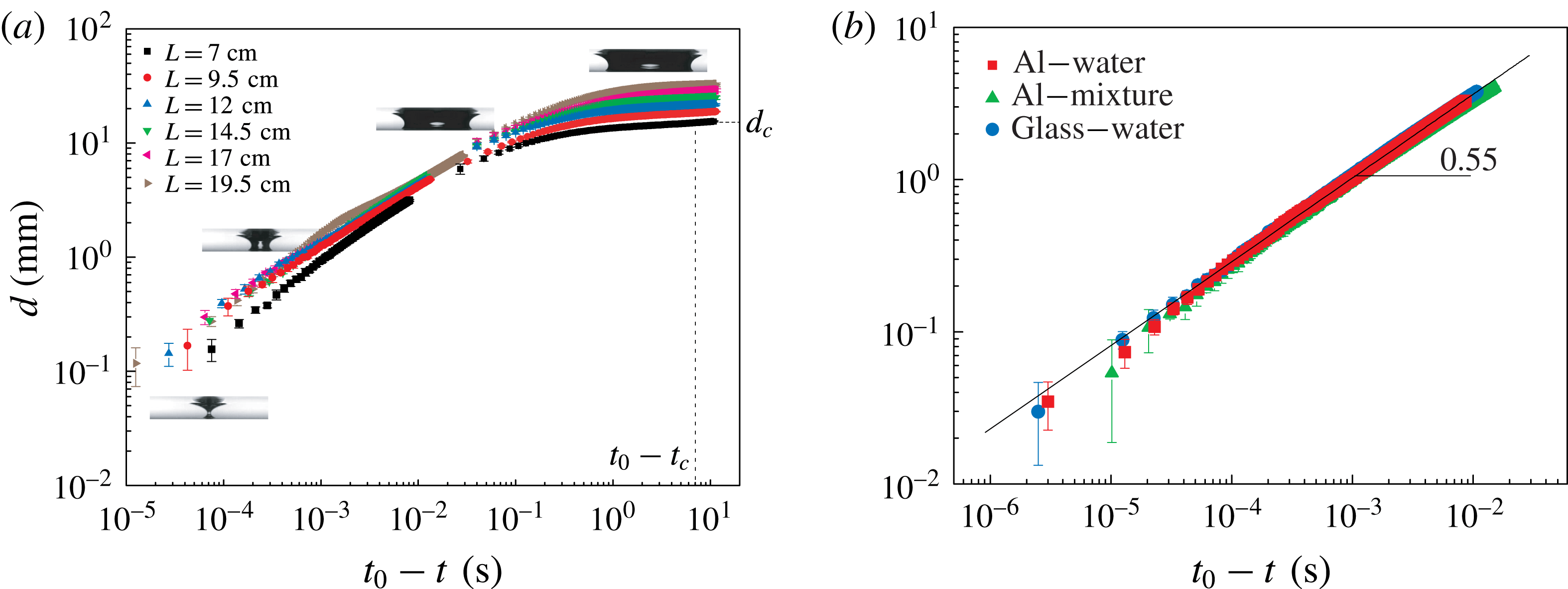
is shown in figure 9 as a log–log plot. We employed a high-speed camera with mainly two different frame rates to capture the initial dynamics (500 f.p.s., right-hand side) and the final stages (73 000 f.p.s., left-hand side), respectively. The first set of experiments was carried out on Al superhydrophobic substrates with different box sizes. To study the influence of the wettability of the substrate, we performed experiments with two different substrates. In figure 9(b), data obtained with a further increased frame rate of 100 000 f.p.s. are shown: the red squares and blue dots represent experiments carried out using superhydrophobic Al plates (
 $L=7$
cm) and liquid-infused glass (
 $L=12$
cm), respectively. It is interesting to note that the hole collapse predominantly obeys a scaling law
 $d=(t_{0}-t)^{0.55}$
, similar to experimental results recently reported for converging fluid films driven by both surface tension and gravitational forcing (Dijksman et al.
Reference Dijksman, Mukhopadhyay, Gaebler, Witelski and Behringer2015). The values for the coefficient
 $c_{1}$
are
 $0.045~\text{m}~\text{s}^{-0.55}$
and
 $c_{1}\approx 0.047~\text{m}~\text{s}^{-0.55}$
for the Al and liquid-infused substrates, respectively. Such a scaling has been recognized as a result of the viscous limit of liquid spreading (Bostwick et al.
Reference Bostwick, Dijksman and Shearer2017). However, in contrast to our work, Bostwick et al. (Reference Bostwick, Dijksman and Shearer2017) performed experiments with silicon oil, having a much higher viscosity than water. A rough estimation of the typical Reynolds number (
 $Re\approx 550$
) in our experiments reveals that inertial forces dominate.
Time evolution of the liquid surface around the point when the hole closes. (a) Superhydrophobic Al substrates have been used in square boxes of different size.
 $d$
as a function of
 $(t_{0}-t)$
is shown in a log–log plot.
 $t_{c}$
and
 $d_{c}$
denote the quantities corresponding to the onset of instability in a box with
 $L=7$
cm. (b) Results on Al surfaces (
 $L=7$
cm) obtained with water (red squares) and water–glycerol mixture (green triangles), together with results on liquid-infused glass (
 $L=12$
cm) obtained with water (blue circles), recorded at 100 000 f.p.s.

In fact, the hole collapse in our experiments is reminiscent of the final stages of the pinch-off of air bubbles in an inviscid liquid, which has been studied quite extensively. Longuet-Higgins, Kerman & Lunde (Reference Longuet-Higgins, Kerman and Lunde1991) demonstrated that the pinch-off dynamics can be captured by a two-dimensional model. It shows that the inertia of the water dominates the asymptotic dynamics, so that the surface tension, viscosity and the influence of the gas may be neglected. In this limit the evolution should approximately follow the power law
 $d\sim t^{0.5}$
, which is supported by simulations and experiments (Longuet-Higgins et al.
Reference Longuet-Higgins, Kerman and Lunde1991; Oguz & Prosperetti Reference Oguz and Prosperetti1993; Burton, Waldrep & Taborek Reference Burton, Waldrep and Taborek2005). Thoroddsen, Etoh & Takehara (Reference Thoroddsen, Etoh and Takehara2007) carried out a systematic experimental study of the pinch-off of a bubble in water and found that the radius
 $d/2$
of the neck of the bubble shrinks with a power law behaviour
 $(d/2)\sim t^{0.57\pm 0.03}$
over more than two decades. Their results are in good agreement with the numerical studies of Leppinen & Lister (Reference Leppinen and Lister2005), who carried out numerical simulations of the break-up of a bubble in an inviscid liquid and observed a pinch-off power law with an exponent
 $0.55\pm 0.01$
. In the analytical works of Gordillo et al. (Reference Gordillo, Sevilla, Rodríguez-Rodríguez and Martinez-Bazan2005) and Eggers et al. (Reference Eggers, Fontelos, Leppinen and Snoeijer2007), the collapse of an axisymmetric cavity in a low-viscosity fluid such as water was studied, in which the surface tension, gas density and viscosity were neglected. They obtained the time-dependent scaling exponents as
 $\unicode[STIX]{x1D6FC}\approx 1/2+1/[-4\ln (t_{0}-t)]$
and
 $\unicode[STIX]{x1D6FC}\approx 1/2+1/[4\sqrt{-\ln (t_{0}-t)}]$
, respectively. Based on the latter expression, Eggers et al. (Reference Eggers, Fontelos, Leppinen and Snoeijer2007) obtained a small increase of the scaling coefficient from 0.55 to 0.57 during collapse. These results also indicate that the dynamics of inviscid bubble pinch-off is not universal, the exact value of the exponent weakly depends on the details of each experiment. In the theoretical model built by Eggers et al. (Reference Eggers, Fontelos, Leppinen and Snoeijer2007), the only two remaining terms in the dynamic equation are inertial. In agreement with Eggers et al. (Reference Eggers, Fontelos, Leppinen and Snoeijer2007), our results indicate that viscosity, the capillary forces and the presence of air inside the hole can be neglected.
 $d\sim (t_{0}-t)^{0.55}$
is consistent with the corresponding theoretical prediction. The capillary forces therefore just trigger the instability, and the final collapse is governed by inertia only. We derived a simplified model (see appendix D) which contains the essentials of the hole closure dynamics.
To further check the influence of viscosity on the dynamics, we measured
 $d$
as a function of
 $(t_{0}-t)$
using a mixture of water and glycerol that is 2.6 times more viscous than pure water. The corresponding data display weak viscous corrections. The details of the results are given in the supplementary material. On the other hand, the value of the Ohnesorge number
 $Oh=\unicode[STIX]{x1D702}/(\unicode[STIX]{x1D70C}\unicode[STIX]{x1D6FE}d)^{1/2}$
, which relates the viscous forces to inertial and surface tension forces, can be estimated. Typically,
 $Oh\approx 0.7\times 10^{-3}$
in our experiments, in which the material properties of pure water at
 ${\sim}25\,^{\circ }\text{C}$
(
 $\unicode[STIX]{x1D702}=0.891\times 10^{-3}$
Pa s,
 $\unicode[STIX]{x1D70C}=997.1~\text{kg}~\text{m}^{-3}$
,
 $\unicode[STIX]{x1D6FE}=0.072~\text{N}~\text{m}^{-1}$
) were used and
 $d=20$
mm was chosen. Even when the diameter of the collapsing hole decreases to
 $d=0.1$
mm, i.e. the resolution limit of our camera, we obtain
 $Oh\approx 0.01$
. These analyses suggest that the influence of viscosity on the hole dynamics can be ignored.
4.2 Evolution of the liquid column after hole collapse
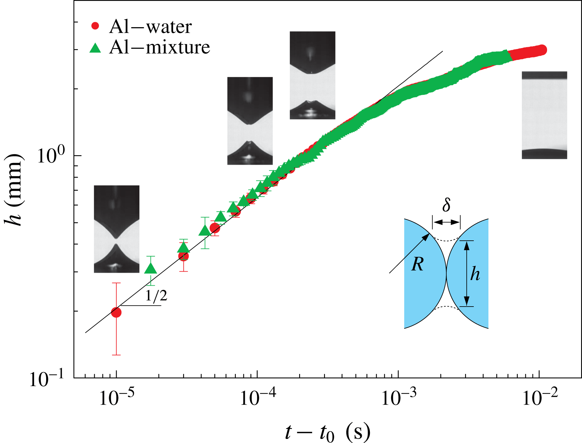
When the hole closes, a growing liquid column separates the gas above from the gas inside the surface bubble. Finally, the liquid gets redistributed into a layer of uniform thickness to minimize the potential energy. Experimental results plotted in figure 10 show that the height of the liquid column
 $h$
shortly after the hole has closed obeys
 $$\begin{eqnarray}h(t)\approx c_{2}\left(\frac{\unicode[STIX]{x1D6FE}l_{c}}{\unicode[STIX]{x1D70C}}\right)^{1/4}(t-t_{0})^{1/2}\end{eqnarray}$$
in which the unknown coefficient has been determined to be
 $c_{2}=3.1$
by fitting.
Compared with the hole collapse discussed in § 4.1, the evolution of the height of the liquid column
 $h$
after hole closure/bubble pinch-off has been studied to a lesser extent. Thoroddsen et al. (Reference Thoroddsen, Etoh and Takehara2007) reported that after pinch-off, the vertical separation of the air cones as a function of time obeys a power law with a fitted exponent of
 $0.49\pm 0.03$
, which is in agreement with the numerics of Leppinen & Lister (Reference Leppinen and Lister2005) who found an exponent of
 $0.48\pm 0.05$
for the evolution of the separation length scale in the breakup of a bubble in an inviscid liquid. The closing of the hole bears a geometrical similarity to the coalescence of droplets or air bubbles (Thoroddsen et al.
Reference Thoroddsen, Etoh, Takehara and Ootsuka2005; Ristenpart et al.
Reference Ristenpart, McCalla, Roy and Stone2006; Bird et al.
Reference Bird, Ristenpart, Belmonte and Stone2009; Courbin et al.
Reference Courbin, Bird, Reyssat and Stone2009; Eddi, Winkels & Snoeijer Reference Eddi, Winkels and Snoeijer2013; Paulsen et al.
Reference Paulsen, Carmigniani, Kannan, Burton and Nagel2014), which has been intensely studied in recent years. For instance, Duchemin, Eggers & Josserand (Reference Duchemin, Eggers and Josserand2003) studied the inviscid coalescence of drops using a boundary integral method. They proposed a power-law scaling for the neck radius as a function of time with an exponent of 0.5. In the work of Thoroddsen et al. (Reference Thoroddsen, Etoh, Takehara and Ootsuka2005), the growth rate of the neck formed after the coalescence of two air bubbles was measured and modelled based on a capillary/inertial balance. A scaling for the neck radius as a function of time with an exponent of 0.5, valid for a comparatively short time interval, was found. Previous results (Eggers, Lister & Stone Reference Eggers, Lister and Stone1999) indicate that already a one-dimensional model captures the underlying physics. For convenience, we model the dynamics in close analogy to the work reported on the coalescence of drops or air bubbles. As shown in the inset of figure 10, during hole closure
 $h^{2}\approx 4\unicode[STIX]{x1D6FF}R$
, denoting by
 $\unicode[STIX]{x1D6FF}$
and
 $R$
the radii of curvature at the ends of the liquid column and of the liquid surface before hole closure, respectively. In our case we have
 $R\approx l_{c}$
. The balance of capillary and inertial forces for a corresponding liquid column leads to
 $2\unicode[STIX]{x1D6FE}/\unicode[STIX]{x1D6FF}\approx (\unicode[STIX]{x1D70C}(h/2t)^{2})/2$
. This results in the functional form of (4.1) with
 $c_{2}=64^{1/4}\approx 2.8$
, showing good agreement to the value obtained from fitting the experimental data.
Time evolution of the liquid column after hole closure.
 $h$
is represented as a function of
 $(t-t_{0})$
in a log–log plot. Each dot represents the average value of five experiments with error bars indicating the standard deviation. The red squares and green triangles represent results obtained on Al surfaces with water and a water–glycerol mixture, respectively. The solid line is the best fit to the experimental data based on the scaling law of (4.1). The snapshots added to specific sections of the curves give an impression of the corresponding shape of the liquid surface. The sketch shows the geometry used for the scaling analysis.

Furthermore, we experimentally studied the influence of viscosity on the evolution of the liquid column (see supplementary material). With a mixture 2.6 time more viscous than water, very similar results were obtained, from which we conclude that the viscosity does not play an important role.
5 Conclusion
We have presented experimental, numerical and theoretical results on the stability and dynamics of holes in bounded liquid layers with a thickness governed by the balance between gravity and capillary forces. Two distinguished regimes were identified, an initial quasi-stationary evolution followed by a dynamic hole collapse beyond the stability threshold. Based on theoretical models and numerical calculations we revealed that the evolution of the hole is controlled by a critical value of the hole diameter below which no stable solution of the Young–Laplace equation exists. This conclusion was corroborated experimentally using substrates with various sizes and wettabilities. The contact angle hysteresis on the employed superhydrophobic and hydrophobic liquid-infused substrates is very small, which largely eliminates the uncertainties resulting from contact line friction (Taylor & Michael Reference Taylor and Michael1973; Bankoff et al. Reference Bankoff, Johnson, Miksis, Schluter and Lopez2003).
From the entirety of the experimental and the theoretical results on hole stability, we can draw the following conclusions. The critical hole diameter increases with increasing box size, but only displays a very weak dependence on the contact angle. For most practical applications, it is tempting to regard a liquid layer as infinitely extended. However, our results show that in the limiting case
 $L\rightarrow \infty$
the critical diameter
 $d_{c}$
is infinite, which contradicts the assumption of an infinite liquid layer. The influence of the shape of the box on the critical hole diameter is negligible.
The dynamics of hole collapse was studied using high-speed imaging. Scaling laws were identified describing the time evolution of the liquid surface during hole collapse. The collapse is governed by a time dependence
 $d\sim t^{0.55}$
, indicating the dominance of inertial effects. It was also found that the thickness of the liquid column forming after the hole has closed obeys a
 $h\sim t^{1/2}$
scaling law. A similar scaling has been observed in the context of coalescence of bubbles or droplets. The role of the viscosity in the final stages of the closure process is negligible, which was verified using a water–glycerol mixture.
Acknowledgements
We would like to thank J. Song for his introduction to the method of producing superhydrophobic Al surfaces. C.L. would like to gratefully acknowledge the support of the Alexander von Humboldt Foundation. We thank D. Lohse, J. Snoeijer, H. A. Stone and J. Eggers for stimulating discussions. We are grateful to the anonymous reviewers whose suggestions have led to a significantly improved paper. C.L. and M.E. contributed equally to this work, and their names in the author list are interchangeable.
Supplementary movies and material
Supplementary movies and material are available at https://doi.org/10.1017/jfm.2018.680.
Appendix A. Materials and experimental methods
A.1 Sample preparation
The superhydrophobic Al surfaces were fabricated based on a method similar to that described in Song et al. (Reference Song, Xu, Liu, Lu and Sun2012). First, Al plates (thickness 2 mm) were cleaned by detergent to remove any oil or dirt. Then, the Al plates were polished with sandpaper (granulation: 500) to remove the oxidation layer and subsequently cleaned with water and acetone. After that, the samples were immersed in
 $4~\text{mol}~\text{l}^{-1}$
aqueous hydrochloric acid (HCl) solution for 8–12 min. Next, after removing the samples from the HCl solution, they were put into an ultrasonic bath for 2 min to remove residual imperfections. After the specimens have been completely dried, they were immersed in 1.0 % (wt/vol) fluoroalkylsilane (FAS) solution for 40 min. Finally, they were kept in an oven at
 $100\,^{\circ }\text{C}$
for 1 h.
The hydrophobic liquid-infused glass surfaces were prepared by the procedure described in Eifert et al. (Reference Eifert, Paulssen, Varanakkottu, Baier and Hardt2014). Firstly, the glass was cleaned by acetone and water in sequence to remove any dirt. Then it was put into a container with silicon oil (5 cSt) which was placed inside an oven. Subsequently, the temperature was increased to
 $300\,^{\circ }\text{C}$
and maintained there for 3 min. Because of evaporation, sufficient silicon oil was required in advance to make sure that the glass was always immersed in the liquid phase. After cooling down, the glass is cleaned using ethanol. Next, the substrate is rinsed with fresh silicon oil (5 cSt). Finally, the glass is fixed in a vertical position for 1 h to remove any excess silicon oil.
The Teflon surfaces were cleaned with ethanol and water. Commercial silicon wafers were used in our experiments without any pre-processing. We could only carry out five experiments on each new silicon wafer. After that the contact angle hysteresis increased, and the used silicon wafers were replaced by new ones to guarantee the repeatability of the experiment. All substrates were precisely cut into the right size to fit into the square boxes.
A.2 Wettability characterization
In all experiments, Milli-Q water was used, either as a pure liquid or in a mixture with glycerol. In order to characterize the wettability of the four different samples used, as well as the Plexiglas surface, we carried out systematic measurements by employing a commercial Krüss DSA 100 (Krüss Company, Ltd. Germany) contact angle measurement apparatus. Specifically, the contact angle
 $\unicode[STIX]{x1D703}$
, the advancing contact angle
 $\unicode[STIX]{x1D703}_{a}$
, and the receding contact angle
 $\unicode[STIX]{x1D703}_{r}$
, were measured, giving the contact angle hysteresis as
 $\unicode[STIX]{x0394}\unicode[STIX]{x1D703}=\unicode[STIX]{x1D703}_{a}-\unicode[STIX]{x1D703}_{r}$
.
 $5~\unicode[STIX]{x03BC}\text{l}$
droplets were created and carefully positioned on the substrates. For superhydrophobic Al and liquid-infused glass substrates, we first produced a
 $5~\unicode[STIX]{x03BC}\text{l}$
droplet, and then translated it along the substrates in order to measure the receding and advancing contact angles. For the Teflon, silicon and the Plexiglas substrates, the advancing and receding contact angles were measured by smoothly increasing and decreasing the volume of the droplet. Each value listed in the following table 1 is the average value of ten measurements with standard deviations.
Wetting properties of the substrates, obtained for water.
Appendix B. Calculations based on the finite element method (FEM)
To verify our assumption that the scenario in a square box can be approximated by an axisymmetric configuration, we resort to FEM simulations. The public domain software package Surface Evolver (SE) (Brakke Reference Brakke1992) was employed to compute the static configuration of the liquid layer in the square boxes.
The basic concept of SE is to minimize the energy and find the equilibrium shape of the surface subjected to the user-defined surface tension, external forces (e.g. gravity) and constraints. SE has been applied for studying various wetting phenomena (Cho et al. Reference Cho, Yi, Lim, Kim, Manoharan, Pine and Yang2005; Kabla & Debregeas Reference Kabla and Debregeas2007; Chou et al. Reference Chou, Hong, Liang, Tsao and Sheng2011; Crawford, Lim & Gradecak Reference Crawford, Lim and Gradecak2013), with excellent agreement to the experimental results.
In our simulations, we first model a square box partially filled with liquid. We apply specific constraints, which means we specify a certain volume
 $V$
of the liquid, we define the contact angles between the liquid and the substrate and with the wall of the box, respectively, and we also initialize a hole at the centre of the liquid. The total energy
 $E$
is defined as
 $$\begin{eqnarray}\displaystyle E & = & \displaystyle E_{s}+E_{g}\nonumber\\ \displaystyle & = & \displaystyle A_{lg}\unicode[STIX]{x1D6FE}+A_{sl}(\unicode[STIX]{x1D6FE}_{sl}-\unicode[STIX]{x1D6FE}_{sg})+\unicode[STIX]{x1D70C}gVh_{c},\nonumber\\ \displaystyle & = & \displaystyle (A_{lg}-A_{sl}\cos \unicode[STIX]{x1D703})\unicode[STIX]{x1D6FE}+\unicode[STIX]{x1D70C}gVh_{c}\end{eqnarray}$$
in which
 $E_{s}$
and
 $E_{g}$
are the surface energy and the gravitational energy, respectively.
 $A_{lg}$
and
 $A_{sl}$
are the areas of the liquid–gas and solid–liquid interfaces. Considering that the contact angle between water and the wall of the box is close to
 $90^{\circ }$
(see table 1), the liquid–wall interface does not contribute to the surface energy, so
 $A_{sl}$
is just the area of the interface between water and the substrate.
 $\unicode[STIX]{x1D6FE}_{sl}$
and
 $\unicode[STIX]{x1D6FE}_{sg}$
are the liquid–solid and solid–gas interfacial tensions.
 $h_{c}$
is the
 $z$
-coordinate of the centre of mass of the liquid. In our simulations, we first specify a value of
 $V$
smaller than the critical volume. After the liquid layer has reached a state of minimal energy, the corresponding value of
 $d$
is obtained. By smoothly increasing the volume
 $V$
, a smaller diameter
 $d$
can be found. For the case that
 $V$
is large enough, during the evolution of the numerical configurations, the hole suddenly disappears, and an equilibrium state (i.e.
 $d<d_{c}$
) with a hole can no longer be found. This indicates that
 $d$
reaches
 $d_{c}$
and
 $V$
reaches
 $V_{c}$
, correspondingly. Following this procedure, we find the dependency of
 $d$
on
 $V,E$
.
The purpose of the SE simulations is to compare the results with the results obtained in the axisymmetric case. For comparison, we first define the nominal surface energy
 $E_{n}$
and volume
 $V_{n}$
for the results obtained with SE, as follows
 $$\begin{eqnarray}\displaystyle & \displaystyle E_{n}=E-(\unicode[STIX]{x0394}E_{s}+\unicode[STIX]{x0394}E_{g}), & \displaystyle\end{eqnarray}$$
 $$\begin{eqnarray}\displaystyle & \displaystyle V_{n}=V-\unicode[STIX]{x0394}V, & \displaystyle\end{eqnarray}$$
in which
 $\unicode[STIX]{x0394}E_{s}$
and
 $\unicode[STIX]{x0394}E_{g}$
are defined as
 $$\begin{eqnarray}\displaystyle \unicode[STIX]{x0394}E_{s} & = & \displaystyle \left[L^{2}-\unicode[STIX]{x03C0}\left(\frac{L}{2}\right)^{2}\right](\unicode[STIX]{x1D6FE}_{sl}-\unicode[STIX]{x1D6FE}_{sg})-\unicode[STIX]{x0394}A_{lg}\unicode[STIX]{x1D6FE}\nonumber\\ \displaystyle & {\approx} & \displaystyle L^{2}\left(1-\frac{\unicode[STIX]{x03C0}}{4}\right)(1-\cos \unicode[STIX]{x1D703})\unicode[STIX]{x1D6FE},\end{eqnarray}$$
 $$\begin{eqnarray}\displaystyle \unicode[STIX]{x0394}E_{g} & = & \displaystyle \unicode[STIX]{x1D70C}g(\unicode[STIX]{x0394}V)h_{ce}\nonumber\\ \displaystyle & {\approx} & \displaystyle \frac{1}{2}\unicode[STIX]{x1D70C}gL^{2}h_{max}^{2}\left(1-\frac{\unicode[STIX]{x03C0}}{4}\right).\end{eqnarray}$$
Here,
 $\unicode[STIX]{x0394}A_{lg}$
and
 $\unicode[STIX]{x0394}V$
denote the liquid surface area and the volume outside of a circular region with diameter
 $L$
, respectively.
 $h_{ce}$
is the centre of mass (
 $z$
-coordinate) of
 $\unicode[STIX]{x0394}V$
. For convenience, we use
 $h_{ce}\approx h_{max}/2$
, in which
 $h_{max}$
is the maximum
 $z$
-coordinate of the liquid surface.
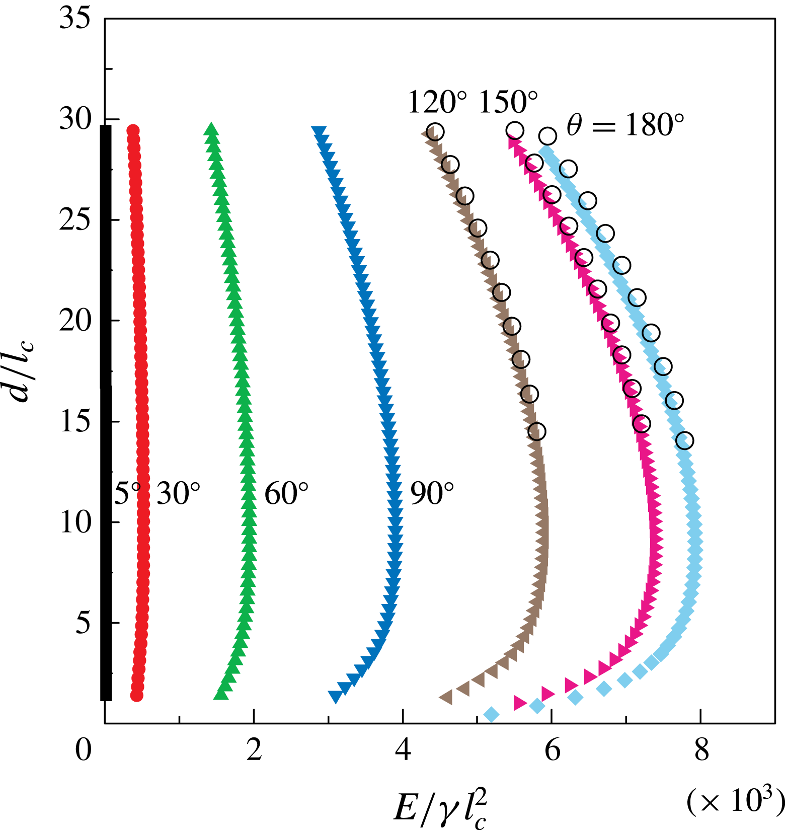
Dependency of
 $E$
on
 $d$
for various wettabilities of the substrate. The numerical solutions of (3.1) are shown as filled symbols. For that case, a circular box with
 $L=14.5$
cm has been considered, with contact angles of
 $\unicode[STIX]{x1D703}=5^{\circ }$
,
 $30^{\circ }$
,
 $60^{\circ }$
,
 $90^{\circ }$
,
 $120^{\circ }$
,
 $150^{\circ }$
,
 $180^{\circ }$
. The black hollow circles have been obtained using surface evolver (the nominal surface energy
 $E_{n}$
), but based on a square box and with contact angles of
 $\unicode[STIX]{x1D703}=120^{\circ }$
,
 $150^{\circ }$
,
 $180^{\circ }$
.

In figure 11, we show the dependency of
 $E$
on
 $d$
in dimensionless form for the box with
 $L=14.5$
cm and various wettabilities of the substrate. The results obtained with SE (the nominal surface energy
 $E_{n}$
) are displayed as hollow black circles, where
 $\unicode[STIX]{x1D703}=120^{\circ }$
,
 $150^{\circ }$
and
 $180^{\circ }$
. Moreover, the comparison between the SE results (i.e.
 $V_{n}$
) and the axisymmetric numerical results with respect to
 $V$
and
 $d$
is reported in figure 5(b). Apparently, a very good agreement between the results obtained with the axisymmetric model and with SE is found, which indicates that the influence of the shape of the bounding box on the evolution of the hole is not appreciable, and provides justification for the assumption of axisymmetry in §§ 3.1 and 3.2.
Appendix C. Extracting the critical diameter
In this section we present a well-defined procedure to extract the critical diameter
 $d_{c}$
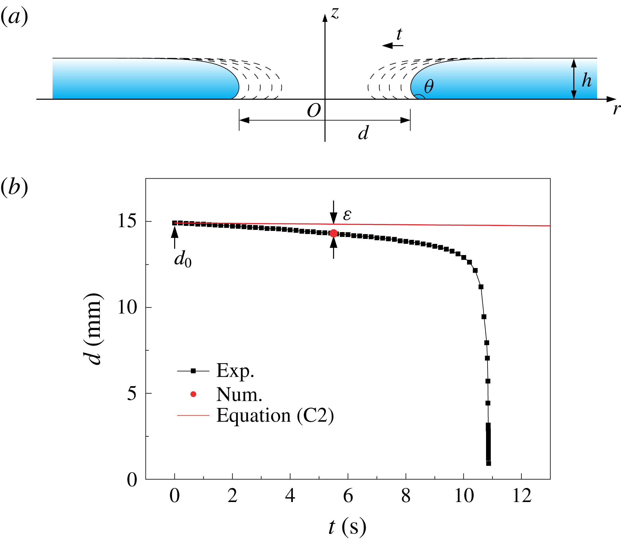
of the collapsing hole from the experimental data. Defining such a procedure is necessary, since from the experimental curves shown in figure 2 the exact values of
 $d_{c}$
do not become immediately apparent. On the other hand, even though specific values of the critical diameter appeared in similar experiments (Taylor & Michael Reference Taylor and Michael1973; Bankoff et al.
Reference Bankoff, Johnson, Miksis, Schluter and Lopez2003; Dijksman et al.
Reference Dijksman, Mukhopadhyay, Gaebler, Witelski and Behringer2015), unfortunately, in none of the corresponding papers was a clear description of how
 $d_{c}$
was extracted from the experimental data given.
We first consider a hole with a diameter significantly larger than the capillary length. In that case, a change in the hole diameter does not induce a significant change in height of the liquid layer. The corresponding configurations with different hole diameters are illustrated in figure 12(a), where
 $h=2l_{c}\sin (\unicode[STIX]{x1D703}/2)$
, corresponding to the height of an infinite liquid layer (de Gennes et al.
Reference de Gennes, Brochard-Wyart and Quéré2003).
Model for the determination of
 $d_{c}$
. (a) Corresponding configurations with different instantaneous hole diameters
 $d(t)$
. The height of the liquid layer is assumed to be constant,
 $h=2l_{c}\sin (\unicode[STIX]{x1D703}/2)$
(de Gennes et al.
Reference de Gennes, Brochard-Wyart and Quéré2003). (b) Procedure for computing the characteristic deviation
 $\unicode[STIX]{x1D700}$
. The black squares are the experimental data obtained in the smallest box (
 $L=7$
cm, see figure 2). The red dot in the diagram represents
 $d_{c}$
as obtained from the numerical results (extracted from figure 7). The solid red line is the result of (C 2).

The symbols for time, hole diameter and liquid volume used in our model are
 $t$
,
 $d$
and
 $V$
, respectively. The rate of volume change in the liquid layer corresponds to the flow rate of the liquid supply, i.e.
 $$\begin{eqnarray}Q=\frac{\text{d}V}{\text{d}t}=-\frac{\unicode[STIX]{x03C0}}{2}l_{c}\sin \left(\frac{\unicode[STIX]{x1D703}}{2}\right)\frac{\text{d}}{\text{d}t}[d^{2}(t)],\end{eqnarray}$$
in which
 $Q=0.1~\text{ml}~\text{min}^{-1}$
is the constant volume rate of the syringe pump. The last equality in (C 1) is based on the assumptions illustrated in figure 12(a). Equation (C 1) can be solved analytically using the boundary condition
 $d|_{t=0}=d_{0}$
, in which
 $d_{0}$
is the initial hole diameter. We arrive at
 $$\begin{eqnarray}d(t)=\sqrt{d_{0}^{2}-\frac{2Q}{\unicode[STIX]{x03C0}l_{c}\sin \left({\displaystyle \frac{\unicode[STIX]{x1D703}}{2}}\right)}t}.\end{eqnarray}$$
To determine the critical hole diameter
 $d_{c}$
from the experimental data, we utilize the procedure described as follows. The relationship of (C 2) is only expected to be valid for situations where the hole diameter is sufficiently larger than the critical diameter. We fit (C 2) to reproduce the rightmost data point (largest value of
 $t_{0}-t$
) of each of the experimental curves shown in figure 2. This can be interpreted as either fixing the choice of
 $d_{0}$
or performing a shift in the time coordinate (for fixed
 $d_{0}$
). The resulting forms of (C 2) (which are different for each value of
 $L$
considered) do not contain any free parameters. Subsequently, it is assumed that the critical hole diameter is reached when the experimental curve deviates by a specific amount from the curve defined by (C 2).
More specifically, the procedure is performed as follows. The experiment carried out in the box with
 $L=7$
cm is taken as a reference. The model curve fitted to the first experimental data point is shown as a solid red line in figure 12(b). For the reasons discussed above, the experimental values for
 $d(t)$
deviate from this curve. The numerical results, shown in figure 7, suggest that in this case the critical diameter takes a value of
 $d_{c}\approx 14.31$
mm, indicated as a red dot in figure 12(b). The deviation between the red dot and the corresponding value of our model
 $d(t_{c})$
can be characterized by defining a dimensionless ratio
 $\unicode[STIX]{x1D700}=(d(t_{c})-d_{c})/d_{c}$
, which takes a value of
 ${\approx}3.74\,\%$
for the considered case. Subsequently, to determine the critical diameter
 $d_{c}$
for the other box sizes, we assume that
 $d_{c}$
is reached when the same deviation of
 $\unicode[STIX]{x1D700}=3.74\,\%$
between the model curve and the experimental data arises. This procedure results in an agreement between the numerical and the experimental data for
 $L=7$
cm per construction, but makes a prediction for
 $d_{c}$
for all other box sizes.
Appendix D. Modelling the hole closure dynamics using a simplified model
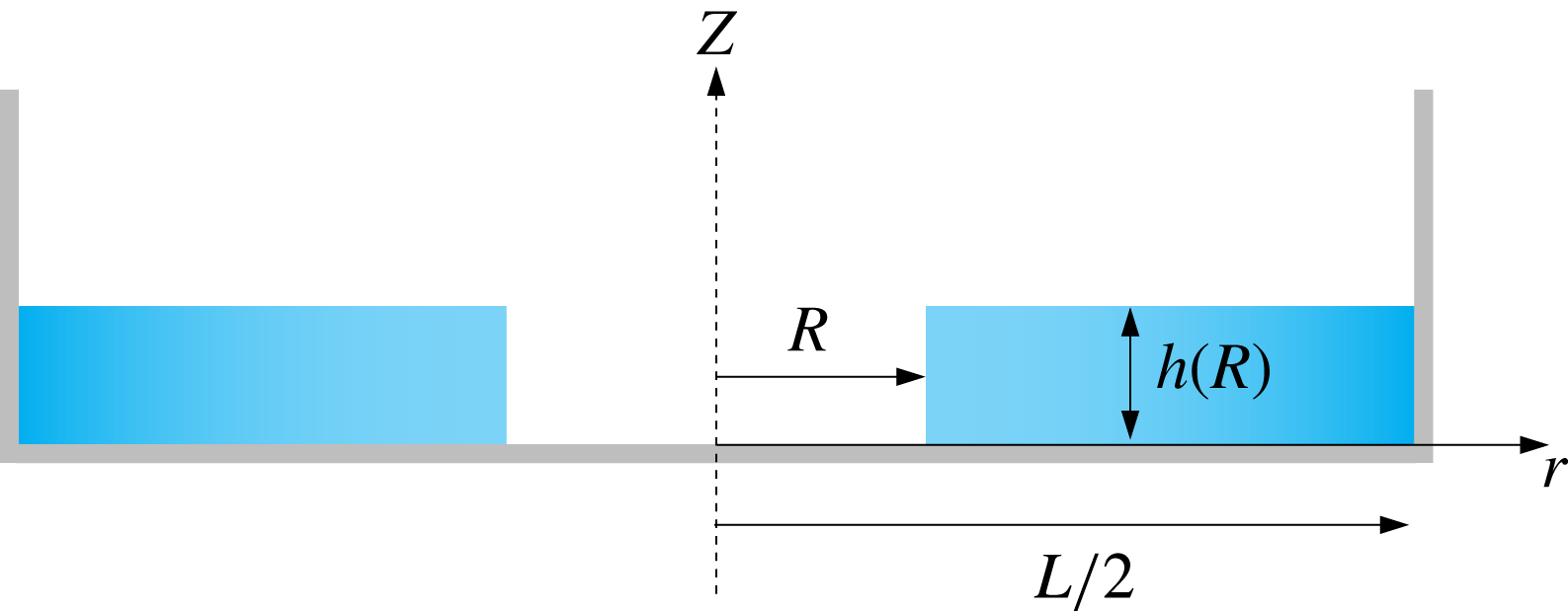
In this section we present a simple model to study the effects governing the hole collapse. For the sake of simplicity, we choose an approach in which we assume that the liquid film has a rectangular cross-section (see figure 13).
Sketch of the rectangular cross-section of a liquid film in a circular container.
 $R(t)$
,
 $h[R(t)]$
are the instantaneous radius of the hole and the thickness of the liquid film, respectively.
 $L$
is the diameter of the container.

We further assume the volume
 $V$
of the liquid to be constant over the time span of the hole collapse
 $V=\unicode[STIX]{x03C0}\left[(L/2)^{2}-R^{2}\right]h(R)$
, so the height
 $h(R)$
of the liquid film can be expressed as
 $$\begin{eqnarray}h(R)=\frac{V}{\unicode[STIX]{x03C0}\left[\left(\displaystyle \frac{L}{2}\right)^{2}-R^{2}\right]}.\end{eqnarray}$$
After integrating the continuity equation (i.e.
 $(1/r)\unicode[STIX]{x2202}(rv_{r})/\unicode[STIX]{x2202}r+\unicode[STIX]{x2202}v_{z}/\unicode[STIX]{x2202}z=0$
) over
 $z\in [0,h(R)]$
, we find
 $$\begin{eqnarray}\int _{0}^{h(R)}\frac{1}{r}\frac{\unicode[STIX]{x2202}}{\unicode[STIX]{x2202}r}(rv_{r})\,\text{d}z+v_{z}[h(R)]-v_{z}(0)=0,\end{eqnarray}$$
in which
 $v_{r}$
and
 $v_{z}$
denote the radial and the vertical velocity, respectively. We neglect viscosity and therefore assume that
 $v_{r}$
is independent of
 $z$
. The vertical velocity at
 $z=0$
vanishes due to the no-penetration condition at the rigid wall. By setting
 $v_{z}[h(R)]=\unicode[STIX]{x2202}h(R)/\unicode[STIX]{x2202}t$
and with the help of (D 1), we arrive at
 $$\begin{eqnarray}v_{r}=\frac{R{\dot{R}}}{r}\left[1-\frac{r^{2}-R^{2}}{\left(\displaystyle \frac{L}{2}\right)^{2}-R^{2}}\right].\end{eqnarray}$$
We denote the time derivative as
 ${\dot{R}}=\unicode[STIX]{x2202}R/\unicode[STIX]{x2202}t$
. It is easy to verify that (D 3) indeed satisfies the no-penetration condition at the vertical wall of the container, i.e. when
 $r=L/2$
.
The energy balance equation reads
 $$\begin{eqnarray}\frac{\unicode[STIX]{x2202}}{\unicode[STIX]{x2202}t}(E_{P}+E_{K})=0,\end{eqnarray}$$
in which
 $E_{P}$
and
 $E_{K}$
are the potential and the kinetic energy, respectively. The potential energy of our system consists of the surface energy and the gravitational energy, and can be written as
 $$\begin{eqnarray}\displaystyle E_{P} & = & \displaystyle \unicode[STIX]{x03C0}\left(\frac{L}{2}\right)^{2}\left[1-\left(\frac{R}{L/2}\right)^{2}\right]\unicode[STIX]{x1D6FE}(1-\cos \unicode[STIX]{x1D703})+2\unicode[STIX]{x03C0}\left(\frac{R}{L/2}\right)\frac{\unicode[STIX]{x1D6FE}V}{\unicode[STIX]{x03C0}\left(\displaystyle \frac{L}{2}\right)\left[1-\left(\displaystyle \frac{R}{L/2}\right)^{2}\right]}\nonumber\\ \displaystyle & & \displaystyle +\,\frac{\unicode[STIX]{x1D70C}V^{2}g}{2\unicode[STIX]{x03C0}\left(\displaystyle \frac{L}{2}\right)^{2}\left[1-\left(\displaystyle \frac{R}{L/2}\right)^{2}\right]}.\end{eqnarray}$$
The first two terms correspond to the surface/interfacial energy of the film, whereas the last term is the gravitational energy. Here, we limit our study to the last moments of the hole collapse, i.e. when
 $R/(L/2)\ll 1$
. By employing a Taylor series expansion and keeping only terms up to the second order in
 $R/(L/2)$
, we obtain
 $$\begin{eqnarray}\displaystyle E_{P} & {\approx} & \displaystyle \unicode[STIX]{x03C0}\left(\frac{L}{2}\right)^{2}\left[1-\left(\frac{R}{L/2}\right)^{2}\right]\unicode[STIX]{x1D6FE}(1-\cos \unicode[STIX]{x1D703})\nonumber\\ \displaystyle & & \displaystyle +\,2\unicode[STIX]{x03C0}\left(\frac{R}{L/2}\right)\frac{\unicode[STIX]{x1D6FE}V}{\unicode[STIX]{x03C0}\left(\displaystyle \frac{L}{2}\right)}+\displaystyle \frac{\unicode[STIX]{x1D70C}V^{2}g}{2\unicode[STIX]{x03C0}\left(\displaystyle \frac{L}{2}\right)^{2}}\left[1+\left(\frac{R}{L/2}\right)^{2}\right].\end{eqnarray}$$
To compute the kinetic energy of the film, the radial velocity has to be obtained at the centre of mass along the radial direction, i.e.
 $r=(L/2+R)/2$
. With the help of (D 3) we obtain
 $$\begin{eqnarray}v_{r}^{com}=\frac{\left(\displaystyle \frac{R}{L/2}\right){\dot{R}}\left(3+\displaystyle \frac{R}{L/2}\right)}{2\left(1+\displaystyle \frac{R}{L/2}\right)^{2}},\end{eqnarray}$$
and the corresponding kinetic energy
 $$\begin{eqnarray}E_{K}=\unicode[STIX]{x1D70C}V\frac{\left(\displaystyle \frac{R}{L/2}\right)^{2}{\dot{R}}^{2}\left(3+\displaystyle \frac{R}{L/2}\right)^{2}}{8\left(1+\displaystyle \frac{R}{L/2}\right)^{4}}\approx \frac{9}{8}\unicode[STIX]{x1D70C}V{\dot{R}}^{2}\left(\frac{R}{L/2}\right)^{2}.\end{eqnarray}$$
If we introduce dimensionless quantities
 $R/(L/2)$
,
 $t/T$
and
 $V/(L/2)^{3}$
, with
 $T$
being a characteristic time scale and inserting (D 6) and (D 8) into (D 4), we get
 $$\begin{eqnarray}1+\bar{R}\left[\unicode[STIX]{x03C0}\frac{\cos \unicode[STIX]{x1D703}-1}{\bar{V}}+Bo\frac{\bar{V}}{2\unicode[STIX]{x03C0}}+\frac{9}{8}We\left(\dot{\bar{R}}^{2}+\bar{R}\ddot{\bar{R}}\right)\right]=0,\end{eqnarray}$$
in which
 $Bo=\unicode[STIX]{x1D70C}g(L/2)^{2}/\unicode[STIX]{x1D6FE}$
and
 $We=\unicode[STIX]{x1D70C}(L/2)^{3}/(\unicode[STIX]{x1D6FE}T^{2})$
are the Bond number, relating the gravitational force to the surface tension force, and the Weber number, relating the inertial force to the surface tension force. Since our model is limited to the situation in which the radius of the hole is small compared to the radius of the container, we choose the characteristic time
 $T=0.01$
s according to our experimental results from figure 9(a), leading to
 $Bo\approx 708$
and
 $We\approx 5.2\times 10^{4}$
, for
 $L=14.5$
cm. We therefore consider equation (D 9) in the limit of high Weber numbers, which leads to
 $$\begin{eqnarray}\bar{R}\ddot{\bar{R}}+\dot{\bar{R}}^{2}=0.\end{eqnarray}$$
A
 $R\sim (t_{0}-t)^{1/2}$
scaling is obtained based on this approximation. This result agrees with the time-independent part (zeroth-order solution) of the solution obtained by Eggers et al. (Reference Eggers, Fontelos, Leppinen and Snoeijer2007).