1. Introduction
Nowadays, unmanned aerial vehicles, especially multirotors, have growingly gained the attention of researchers in automatic control area due to their advantages such as vertical takeoff and landing, rapid maneuvering, precise hovering, simple structure, and their capability in performing various tasks, ranging from aerial manipulation, search and rescue, security and inspection.
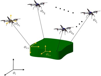
Cooperative load transportation is another important application of drones studied by researchers [Reference Vahdanipour and Khodabandeh1–Reference Shirani, Najafi and Izadi5]. This is considered when the payload is bulky or heavy, and it is impossible for one robot to handle it (Fig. 1). However, in comparison with a single robot, the cooperation associated with multiple robots makes the problem complicated. The problem is more complex when the payload is nonuniform (mass distribution of the payload is not uniform and consequently its Center of Gravity [CG] is not located at the geometric center) and the mass and location of the center of mass are also unknown. Although these unknown physical parameters can be estimated using force or torque sensors, but using these sensors in small robots are limited for being expensive and heavy. Therefore, the main objective of this paper is to develop a control algorithm to estimate the force on the rope attached to each quadrotor without using force or torque sensors. Based on this estimation, an algorithm is presented to determine the unknown physical parameters of the payload including mass and CG position. This is essential in determining the optimal formation of robots around the payload which will be discussed in Section 5.
Cooperative load transportation.

The literature on the load transportation with a single aerial robot is rich, and different control algorithms have been investigated in the past [Reference Wang, Song, Huang and Tang6–Reference Pierri, Muscio and Caccavale11]. In ref. [Reference Wang, Song, Huang and Tang6] a hierarchical nonlinear control to track a 3D trajectory subject to payload variation and fast time-varying wind gust disturbance was proposed. Dai et al. proposed an adaptive controller for a quadrotor Unmanned Aerial Vehicle (UAV) transporting an unknown mass-point payload connected by a flexible cable [Reference Dai, Lee and Bernstein7]. The problem of transporting a cable-suspended payload using a quadrotor was presented in ref. [Reference Cruz and Fierro8]. Unlike other papers that have assumed the system is always in the air and the cable is always taut, they have assumed that the cable is not taut at first. Therefore, they analyzed the lifting maneuver, when the cable goes instantaneously from slack to taut condition. In ref. [Reference de Angelis9] a filtering technique has been presented to estimate swing angle for multicopter slung load applications. The estimation of swing angle was based on the data available from the onboard inertial measurement unit. A trajectory control scheme for handling a payload by an aerial robot was presented in ref. [Reference de Angelis, Giulietti and Pipeleers10]. They modeled the load as a pendulum that is connected to the CG of the robot.
However, when the payload is heavy, a single robot cannot handle the load. Therefore, the cooperative load transportation should be considered for heavy loads. Cooperative transportation and manipulation can be used in various applications such as production lines, construction sites, or remote operations. In many researches, this purpose was achieved by using ground robots or aerial robots.
In ref. [Reference Yoshikawa12], a coordinated dynamic hybrid control method for multi-fingered mechanisms was proposed. In ref. [Reference Sieber, Deroo and Hirche13], transporting an object in a centralized method was presented. They solved an optimal linear state feedback controller iteratively for cooperative manipulation. In ref. [Reference Mellinger, Shomin, Michael and Kumar14], they presented a centralized controller to grasp and transport a payload in a three dimensional space. They used a gripping mechanism in each quadrotor that enabled autonomous grasping of the payload. In ref. [Reference Fink, Michael, Kim and Kumar15], planning and control of multiple aerial robots manipulating and transporting a payload in three dimensions via cables were presented. For a triangular payload, they presented a numerical solution to determine feasible equilibrium of the payload. Yang et al. presented a hierarchical control framework for multiple agents equipped with a 2-DoF (Degree of Freedom) robotic arm for aerial manipulation [Reference Yang and Lee16]. They solved a constrained quadratic optimization problem to compute cooperative force distribution among the robotic arms. The dynamics and control of quadrotor UAVs transporting a rigid body payload connected via flexible cables were discussed in ref. [Reference Goodarzi and Lee17]. A multilevel and distributed control system, based on a robust model predictive control technique, for a multi-body slung-load system was presented in ref. [Reference Tartaglione, D’Amato, Ariola, Rossi and Johansen18].
In refs. [Reference Dong19, Reference Xiao, Yin and Kaynak20], uncertainty for the payload has been considered. In these studies, the uncertain parameters of the payload were handled, but they focused on a single manipulator. In refs. [Reference Aghili21, Reference Monfaredi, Rezaei and Talebi22], a control scheme to handle inaccurate kinematic model of payload such as inaccurate orientation and length at the gripping point has been presented. In these works, it has been supposed that physical parameters of payload were known. Lee et al. presented a parameter-robust controller for transportation a payload by multiple aerial robots [Reference Lee, Yoo, Lee, Moon, Lee, Tahk and Shin23]. They showed that their controller is robust against variation of payload mass. Hybrid force/position control architecture for object transportation by a mobile robot formation was presented in ref. [Reference Neumann and Kitts2]. For ground mobile robots, in ref. [Reference Franchi, Petitti and Rizzo24] estimation of kinematic and inertial parameters of an unknown rigid body in a distributed approach was presented. Estimation was done by using each robot measurements of its velocity and contact forces applied to the load. A distributed adaptive coordinated control method for multiple robotic arms grasping a common object was considered in ref. [Reference Kawasaki, Ueki and Ito25]. In this paper, the dynamic parameters of both object and robot arms were estimated adaptively. The algorithm used does not use any force sensor measurement, but it requires the measurements of the positions and velocities of the object and robotic arms. In ref. [Reference Lee and Kim26], the problem of cooperative aerial manipulators to carry an unknown object has been considered. In this paper, the aerial robot is a hexacopter equipped with a robotic arm. The authors have presented an adaptive sliding controller to estimate the unknown mass and inertia of the load for a homogenous payload.
The main contribution of this paper are as follows: (1) unlike previous research, payload dynamics have not been used in the controller design. Therefore, the robotic team is capable of carrying any load in any size, shape and weight without compromising performance. (2) We propose a novel method for estimating the following parameters of the payload: Three components of CG, weight, attitude, and position. (3) In the previous research, it is assumed that the payload is uniform or is like a point mass, while in fact, the payload is nonuniform. (4) We will show that quadrotors positions in a formation flight for load transportation should be determined considering the payload CG information, otherwise the system’s efficiency will be reduced greatly. (5) In the previous research, The Udwadia–Kalaba equations have been developed for a homogenous payload, while we develop these equations for a nonuniform payload for the first time. (6) The proposed algorithm is not limited by the number of quadrotors and can easily be extended to a large number of agents carrying a payload.
The rest of the paper is organized as follows. The dynamic modeling of quadrotors and the payload including the rope constraints is presented in Section 2. The control and estimation algorithms are discussed in Sections 3 and 4. The simulation results are presented in Section 5, and Section 6 concludes this paper.
2. Dynamic Modeling
In this section, the dynamic model of a multi-body slung load system is presented. Figure 1 shows the configuration of the n quadrotors connected to the payload by the ropes. Here, four reference frames are used to describe the position and attitude of the quadrotors and the payload: (1) the inertial frame defined as
 ${O_I}$
, (2) the body fixed frame attached to the CG of the payload described as
 ${O_{p,1}}$
, (3) the body fixed frame attached to the first attachment point of the payload described as
 ${O_{p,2}}$
, and (4) the body fixed frame attached to the CG of the quadrotor described as
 ${O_Q}$
. The quadrotors and payload are modeled as a 6-DoF rigid body in the space.
2.1. Quadrotor dynamics model
The position vector of the center of
 ${O_Q}$
frame with respect to
 ${O_I}$
is defined as
 $\xi^{[i]}(t)=[x(t),y(t),z(t)]^{T}\in\mathbb{R}^{3}$
. The attitude vector with respect to
 ${O_I}$
is defined as
 $\Phi^{[i]}(t)=[\phi(t),\theta(t),\psi(t)]^{T}\in\mathbb{R}^{3}$
. According to these definitions, the equation of the motion of the i
th quadrotor with respect to
 ${O_I}$
can be obtained as follows:
 \begin{align} m_q^{[i]}{\ddot \xi ^{[i]}} + K_\xi ^{[i]}{\dot \xi ^{[i]}} + m_q^{[i]}G = R_t^{[i]}(\Phi ){F^{[i]}} - {T^{[i]}}{J^{[i]}}({\Phi ^{[i]}}){\ddot \Phi ^{[i]}} + (C_m^{[i]}({\Phi ^{[i]}},{\dot \Phi ^{[i]}}) + K_r^{[i]}){\dot \Phi ^{[i]}} + d_\Phi ^{[i]} = {\tilde \tau ^{[i]}}\end{align}
where
 ${m_q}$
is the mass of the quadrotor,
 ${K_\xi } = {\left[ {{K_x},{K_y},{K_z}} \right]^T}$
is the matrix of the translational aerodynamic damping coefficients, and
 $G = {\left[ {0,0,g} \right]^T}$
denotes the gravity acceleration vector with
 $g\in\mathbb{R}^{+}$
. The rotational matrix from
 ${O_Q}$
to
 ${O_I}$
is defined by
 ${R_t}({{\Phi }}) \in SO\left( 3 \right)$
.
 $F = {\left[ {0,0,u(t)} \right]^T}$
denotes thrust force vector,
 ${T^{\left[ i \right]}}$
is the tension vector on the rope between i
th quadrotor and the payload,
 $J({{\Phi }})$
is the inertial matrix defined in the inertial frame,
 ${C_m}({{{\Phi }},{{\dot \Phi }}})$
denotes the Coriolis matrix,
 ${K_r}({{\Phi }})$
is the matrix of the velocity transformation from
 ${O_Q}$
to
 ${O_I}$
,
 ${d_{{\Phi }}} = {\left[ {{d_1}(t),{d_2}(t),{d_3}(t)} \right]^T}$
represents the external disturbances, and
 $\tilde \tau $
denotes the generalized control torque input in the inertial frame. The detailed information of
 $J({{\Phi }})$
,
 ${C_m}({{{\Phi }},{{\dot \Phi }}})$
, and
 ${R_t}({{\Phi }})$
can be found in ref. [Reference Kendoul, Yu and Nonami27].
The dynamic equations defined in Eq. (1) are coupled and
 ${R_t}({{\Phi }})$
is the coupling term. In order to decouple the two connected systems, the virtual control input Q is defined. Therefore, Eq. (1) can be rewritten as
 $$\matrix{
\matrix{
{\chi ^{[i]}} = {\Pi _1}{x^{[i]}} + {\Pi _2}\left( { - {K_\xi }{{\dot \xi }^{\left[ i \right]}}/m_q^{[i]} + {T^{\left[ i \right]}}/m_q^{[i]} + Q - \dot \xi _d^{[i]}} \right) + {\Pi _2}\left( { - G - Q + R_t^{\left[ i \right]}\left( {{\Phi ^{\left[ i \right]}}} \right){F^{\left[ i \right]}}/m_q^{\left[ i \right]}} \right) \hfill \cr
\,\,\,\,\,\,\,\,\,\,\,\,\,\,\,\,\,\,\,\,\,\,\,\,\,\,\,\,\,\,\,{{\dot \varepsilon }^{[i]}} = {\Pi _1}{\varepsilon ^{[i]}} + {\Pi _2}\left( { - \ddot \Phi _d^{[i]} + {J^{{{[i]}^{ - 1}}}}\left( {\left( { - C_m^{[i]}\left( {{\Phi ^{[i]}},{{\dot \Phi }^{[i]}}} \right) + K_r^{[i]}} \right){{\dot \Phi }^{[i]}}} \right) + \tilde \tau - {d_\Phi }} \right) \hfill \cr} \hfill \cr } $$
where
 $\xi^{[i]}_{d}\in\mathbb{R}^{3}$
is the desired position trajectory and
 $\Phi^{[i]}_{d}\in\mathbb{R}^{3}$
is the desired attitude trajectory. The tracking errors
 ${\chi ^{\left[ i \right]}}$
,
 ${\varepsilon ^{\left[ i \right]}}$
, and
 ${\Pi _1}$
,
 ${\Pi _2}$
are defined as follows:
 \begin{align*} {\chi ^{\left[ i \right]}} = {\left[ {{{\left( {{\xi ^{\left[ i \right]}} - \xi _d^{\left[ i \right]}} \right)}^T},{{\left( {{{\dot \xi }^{\left[ i \right]}} - \dot \xi _d^{\left[ i \right]}} \right)}^T}} \right]^T}\end{align*}
 \begin{align*} {\varepsilon ^{\left[ i \right]}} = {\left[ {{{\left( {{\varepsilon ^{\left[ i \right]}} - \varepsilon _d^{\left[ i \right]}} \right)}^T},{{\left( {{{\dot \varepsilon }^{\left[ i \right]}} - \dot \varepsilon _d^{\left[ i \right]}} \right)}^T}} \right]^T}\end{align*}
 $${\Pi _1} = \left[ {\matrix{
{{O_3}\;\;\;\;} & {{I_3}} \cr
{{O_3}} & {\;\;\;\;{O_3}} \cr } } \right]{\Pi _2} = [{O_3}\;\;\;\; \vdots \;\;\;\;{I_3}].$$
A quadrotor is an underactuated system, and this makes its position and attitude control challenging. Thus, the desired trajectory for positions and
 $\psi $
are defined, and the desired values for
 $\theta $
,
 $\phi $
, and the total thrust force
 $u(t)$
are determined by the solutions of
 $Q = \left[ {{Q_1},{Q_2},{Q_3}} \right]$
as follows:
 $$\matrix{
{{\rm{sin}}\left( {\phi _d^{\left[ i \right]}} \right) = m_q^{\left[ i \right]}\left( {Q_1^{\left[ i \right]}{\rm{sin}}\psi _d^{\left[ i \right]} - Q_2^{\left[ i \right]}{\rm{cos}}\psi _d^{\left[ i \right]}} \right)/u_t^{[i]}{\rm{ }}} \hfill \cr
{{\rm{tan}}\left( {\theta _d^{\left[ i \right]}} \right) = \left( {Q_1^{\left[ i \right]}{\rm{cos}}\psi _d^{\left[ i \right]} + Q_2^{\left[ i \right]}{\rm{sin}}\psi _d^{\left[ i \right]}} \right)/Q_3^{\left[ i \right]} + g} \hfill \cr
{\,\,\,\,\,\,\,\,\,\,\,\,\,\,\,\,\,u_t^{\left[ i \right]} = m_q^{\left[ i \right]}\sqrt {Q_1^{{{\left[ i \right]}^2}} + Q_2^{{{\left[ i \right]}^2}} + {{\left( {Q_3^{\left[ i \right]} + g} \right)}^2}} .} \hfill \cr } $$
The effects of actuator system can be described by Eq. (3) as follows:
 $$\matrix{
\matrix{
\,\,\,\,\,\,\,\,u_t^{\left[ i \right]} = f_1^{\left[ i \right]} + f_2^{\left[ i \right]} + f_3^{\left[ i \right]} + f_4^{\left[ i \right]} \hfill \cr
\,\tau _x^{\left[ i \right]} = {l^{\left[ i \right]}}\left( { - f_1^{\left[ i \right]} - f_2^{\left[ i \right]} + f_3^{\left[ i \right]} + f_4^{\left[ i \right]}} \right) \hfill \cr
\,\tau _y^{\left[ i \right]} = {l^{\left[ i \right]}}\left( { - f_1^{\left[ i \right]} + f_2^{\left[ i \right]} + f_3^{\left[ i \right]} - f_4^{\left[ i \right]}} \right) \hfill \cr
\tau _z^{\left[ i \right]} = {c^{\left[ i \right]}}\left( { - f_1^{\left[ i \right]} + f_2^{\left[ i \right]} - f_3^{\left[ i \right]} + f_4^{\left[ i \right]}} \right), \hfill \cr} \hfill \cr } $$
where
 ${\,f_j}\;{{j = 1,}}\cdots{{,4}}$
is the force generated by the
 ${j^{{\rm{th}}}}$
component of the actuator system. Two parameters
 $l$
and
 $c$
are the moment arm and yaw moment factor which convert the force to moment vector.
2.2. Payload dynamic model
The payload dynamics is discussed here in order to develop a suitable simulation framework for cooperative payload transportation problem. Therefore, the payload dynamics will not be used in the controller design for quadrotors. It is assumed that the payload is on the ground at first; therefore the dynamics of the payload has a switching point. The payload is on the ground until the sum of the forces acting on the load in the z direction is less than the payload weight. Based on this condition, the dynamics of the payload can be written as
 $$\matrix{
{{m^{[L]}}{{\ddot \xi }^{[L]}}} \hfill & { + {K^{[L]}}{{\dot \xi }^{[L]}} + {m^{[L]}}G = T + N} \hfill \cr
{{J^{[L]}}({\Phi ^{[L]}}){{\ddot \Phi }^{[L]}}} \hfill & { + \left( {C_m^{[L]}\left( {{\Phi ^{[L]}},{{\dot \Phi }^{[L]}}} \right) + K_r^{[L]}} \right){{\dot \Phi }^{[L]}} + d_\Phi ^{[L]} = {M_L}} \hfill \cr } $$
where
 ${m^{[L]}} \in {\mathbb {R}^ + }$
is the mass of the payload,
 $T = \left[ {{T_x},{T_y},{T_z}} \right] = - \mathop \sum \nolimits_{i = 1}^{{n_q}} {T_i}$
is the sum of the tensions on the ropes connected to the quadrotors,
 ${M_L}$
is the moments of the ropes around CG of the payload, and N represents the ground reaction force and can be defined as
 $$\matrix{
{\left\{ {\matrix{
{N = {m^{[L]}}G - T\;\;\;\;\;\;\;\;} & {\left\| T \right\| \le \left\| {{m^{[L]}}G} \right\|} \cr
{[4pt]N = 0\;\;\;\;\;\;\;\;} & {\left\| T \right\|{\rm{ > }}\left\| {{m^{[L]}}G} \right\|} \cr } } \right.} \hfill \cr } $$
2.3. Multi-body dynamic model
The Udwadia–Kalaba equation is here used to calculate the constraint forces on the ropes acting on each quadrotor [Reference Udwadia and Kalaba28]. It was assumed that ropes are taut and their length is constant. This constraint can be written as
 \begin{align} {g^{\left[ i \right]}} = {\left( {{\xi ^{\left[ i \right]}} - p_I^{\left[ i \right]}} \right)^T}\left( {{\xi ^{\left[ i \right]}} - p_I^{\left[ i \right]}} \right) - L_{rope}^{{{\left[ i \right]}^2}}\end{align}
where
 $p_I^{\left[ i \right]}$
is the
 ${i^{{\rm{th}}}}$
rope attachment point on the payload in the inertial frame. Now,
 ${g^{\left[ i \right]}}$
can be differentiated twice, and we have
 $$\matrix{
{{{\dot g}^{\left[ i \right]}}} \hfill & { = 2{{\left( {{{\dot \xi }^{\left[ i \right]}} - \dot p_I^{\left[ i \right]}} \right)}^T}\left( {{{\dot \xi }^{\left[ i \right]}} - p_I^{\left[ i \right]}} \right){\rm{ }}} \hfill \cr
{{{\ddot g}^{[i]}}} \hfill & { = 2{{({{\ddot \xi }^{[i]}} - \ddot p_I^{[i]})}^T}({\xi ^{[i]}} - p_I^{[i]}) + 2{{({{\dot \xi }^{[i]}} - \dot p_I^{[i]})}^T}({{\dot \xi }^{[i]}} - \dot p_I^{[i]})} \hfill \cr } $$
 $p_I^{\left[ i \right]}$
should be replaced by
 \begin{align} p_I^{\left[ i \right]} = {\xi ^{\left[ L \right]}} + {R^{\left[ L \right]}}p_B^{\left[ i \right]},\end{align}
where
 $p_B^{\left[ i \right]}$
is the
 ${i^{{\rm{th}}}}$
rope attachment point on the payload in the body frame. Therefore, Eq. (8) can be rewritten as
 \begin{align} {\ddot g^{[i]}} = 2{(^{{{\dot \xi }^{[i]}}}}({\xi ^{[i]}} - {\xi ^{[L]}} - {R_L}p_B^{[i]}) + 2{(^{{{\dot \xi }^{[i]}}}}({\dot \xi ^{[i]}} - {\dot \xi ^{[L]}} - {\dot R_L}p_B^{[i]})\end{align}
In order to use Udwadia–Kalaba equation, Eq. (10) can be rewritten as follows:
 \begin{align} {A^{[i]}}(q,\dot q)\ddot q = {B^{[i]}}(q,\dot q) \end{align}
where
 \begin{align} q = {\left[ {\begin{array}{*{20}{c}}{{\xi ^{\left[ 1 \right]}}}\quad{{\xi ^{\left[ 2 \right]}}}\quad \cdots \quad{{\xi ^{\left[ n \right]}}}\quad{{\xi ^{\left[ L \right]}}}\quad{{\phi ^{\left[ L \right]}}}\quad{{\theta ^{\left[ L \right]}}}\quad{{\psi ^{\left[ L \right]}}}\end{array}} \right]^T}\end{align}
 \begin{align*} {A^{\left[ i \right]}} = \left[ {{{\rm{O}}_{1 \times 3\left( {i - 1} \right)}}({\xi ^{\left[ i \right]}} - {\xi ^{\left[ L \right]}}} \right){{\rm{O}}_{1 \times 3\left( {n - i} \right)}} - {\left( {{\xi ^{\left[ i \right]}} - {\xi ^{\left[ L \right]}}} \right)^T}\,A_{3\left( {n + 1} \right) + 1}^{\left[ i \right]}\;A_{3\left( {n + 1} \right) + 2}^{\left[ i \right]}\;A_{3\left( {n + 1} \right) + 3}^{\left[ i \right]}].\end{align*}
The detail of  $A_{3\left( {n + 1} \right) + 1}^{\left[ i \right]},\;A_{3\left( {n + 1} \right) + 2}^{\left[ i \right]},\;A_{3\left( {n + 1} \right) + 3}^{\left[ i \right]}$
and
 ${B^{\left[ i \right]}}\left( {q,\dot q} \right)$
can be found in Appendix. Therefore, the complete constraint equation can be written as
 \begin{align} A = \left[ \begin{matrix} {{A^{\left[ 1 \right]}}} \\ {{A^{\left[ 2 \right]}}} \\ \vdots \\ {{A^{\left[ n \right]}}} \end{matrix} \right]B = \left[ \begin{matrix} {{B^{\left[ 1 \right]}}} \\ {{B^{\left[ 2 \right]}}} \\ \vdots \\ {{B^{\left[ n \right]}}} \end{matrix} \right]\end{align}
As proved in Sieber et al., the constraint forces can be obtained as
 ${Q_c} = {M^{1/2}}{\left( {A{M^{ - 1/2}}} \right)^{\unicode{x2020}} }\left( {B - A{{\ddot q}_u}} \right)$
where
 \begin{align} M = diag\left\{ {{m^1}{I_3},{m^{[2]}}{I_3},...,{m^{[n]}}{I_3},{m^{[L]}}{I_3},{J^{[L]}}} \right\}\end{align}
It can be seen that Eq. (15) satisfies only the acceleration constraints. Therefore, a position drift can occur. Thus, as suggested in ref. [Reference Baumgarte29], Eq. (14) can be modified as
 $${Q_c} = {M^{1/2}}{\left( {A{M^{ - 1/2}}} \right)^{\unicode{x2020}} }\left( {B - 2\alpha \dot g - {\beta ^2}g - A{{\ddot q}_u}} \right)$$
where
 $\alpha \in \mathbb{R}^{+}$
and
 $\rho \in {\mathbb {R}^ + }$
are constants. Therefore, Eq. (16) is used to develop the multi-body load transportation simulator.
3. Control System
In this section, two independent laws are developed for the outer-loop and inner-loop control of the quadrotor. For the outer loop or position loop, the invariance and immersion (I&I) adaptive control is utilized, because the tension on the rope attached to the quadrotor should be estimated and compensated. For the inner loop or attitude loop, an I&I is also used to compensate external disturbance torques.
3.1 Outer-loop control
The main idea of this subsection is to design a tracking controller for the outer-loop system which ensures the asymptotical convergence of the tracking error to zero and correspondingly the estimated rope tensions to their actual values. If the rope tensions are estimated precisely, then the attachment point on the payload can be estimated as well. The dynamics of the outer loop can be written as
 \begin{align} \ddot \xi = - {1 \over {{m_q}}}{K_\xi }\dot \xi - {1 \over {{m_q}}}T + Q\end{align}
In order to simplify the stability analysis and reduce the system order, the position error
 ${e_\xi }(t) = {\left[ {{e_x}(t),{e_y}(t),{e_z}(t)} \right]^T} \in {\mathbb {R}^3}$
and its filtered error signal
 ${r_\xi }(t) = {\left[ {{r_x}(t),{r_y}(t),{r_z}(t)} \right]^T} \in {\mathbb {R} ^3}$
are expressed as
 \begin{align} {e_\xi } = \xi - {\xi _d},\;\;\;{{\rm{r}}_\xi } = {\dot e_\xi } + \sigma {e_\xi },\end{align}
where
 $\sigma = diag\left\{ {{\sigma _x},{\sigma _y},{\sigma _z}} \right\} \in {\mathbb {R}}_ + ^{3 \times 3}$
is a diagonal matrix with positive control gains. The state-space form can be written as follows by substituting Eq. (18) into Eq. (17):
 $$\matrix{
{{{\dot e}_\xi }} \hfill & { = - \sigma {e_\xi } + {r_\xi }{\rm{ }}} \hfill \cr
{{{\dot r}_\xi }} \hfill & { = Q - {1 \over {{m_q}}}\omega + \sigma {{\dot e}_\xi } - {1 \over {{m_q}}}{K_\xi }\dot \xi ,} \hfill \cr } $$
where
 $\omega = T \in {\mathbb {R}^3}$
is the adaptive term. Different from the classic adaptive control theory, the I&I method consists of two parts: the dynamic part
 $\dot \omega $
and the auxiliary part
 $\beta \left( . \right)$
. Therefore, we should design both the update law of
 $\dot \omega $
and the auxiliary function
 $\beta \left( . \right)$
.
Motivated by ref. [Reference Zhao, Xian, Zhang and Zhang30], the estimation error
 $\zeta (t) = {\left[ {{\zeta _x}(t),{\zeta _y}(t),{\zeta _z}(t)} \right]^T}$
can be defined as
 \begin{align} \zeta (t) = \widehat{\omega} - \omega + \beta \left( {{e_\xi },{r_\xi }} \right),\end{align}
where
 $\widehat{\omega} = {\left[ {{{\widehat{\omega} }_x},{{\widehat{\omega} }_y},{{\widehat{\omega} }_z}} \right]^T}$
denotes the dynamic part and
 $\beta ({r_\xi }) \in {\mathbb {R}^3}$
is the auxiliary part defined as follows:
 \begin{align} \beta \left( {{r_\xi }} \right) = - \frac{1}{{{m_q}}}{r_\xi },\end{align}
where
 $\gamma = diag\left\{ {{\gamma _x},{\gamma _y},{\gamma _z}} \right\} \in {\mathbb R}_ + ^{3 \times 3}$
is the positive gain matrix. Assuming
 $\omega $
is constant, Eq. (20) can be differentiated with respect to time to obtain the dynamics for
 $\zeta (t)$
 \begin{align} \dot \zeta = \dot{\widehat{\kern-0.2pt\omega}} - {1 \over {{m_q}}}\gamma \left(Q - {1 \over {{m_q}}}(\widehat{\omega}+ \beta - \zeta ) + \sigma {\dot e_\xi } - {1 \over {{m_q}}}{K_\xi }\dot \xi \right).\end{align}
Therefore, based on Eq. (22), the control input Q and the adaptive state feedback update law
 $\dot{\widehat{\omega}} $
can be determined by
 \begin{align} Q = - {k_p}{r_\xi } + \frac{1}{{{m_q}}}\left( {\widehat{\omega} + \beta } \right) - \sigma {\dot e_\xi } + \frac{1}{{{m_q}}}{K_\xi }\dot \xi \end{align}
 \begin{align} \dot{\widehat{\kern-0.2pt\omega}} = {1 \over {{m_q}}}\gamma (Q - {1 \over {{m_q}}}(\widehat{\omega} + \beta ) + \sigma {\dot e_\xi } - {1 \over {{m_q}}}{K_\xi }\dot \xi ),\end{align}
where
 ${k_p} = diag\left\{ {{k_x},{k_y},{k_z}} \right\} \in {\mathbb R}_ + ^{3 \times 3}$
is a positive gain matrix. Substituting these equations into Eq. (22), it can be obtained that
 \begin{align} \dot \zeta = - \frac{1}{{m_q^2}}\gamma \zeta, \end{align}
and the state-space system in Eq. (19) can be rewritten as
 \begin{align} \begin{matrix} {{{\dot e}_\xi } = - \sigma {e_\xi } + {r_\xi }} \\[4pt] {{{\dot r}_\xi } = - {k_p}{r_\xi } + {1 \over {{m_q}}}\zeta } \end{matrix}. \end{align}
Theorem 1. If the control gain matrices
 ${k_p}$
and
 $\sigma$
are selected properly, the control input Q, the adaptive state feedback update law in Eqs. (23) and (24), and the auxiliary function in Eq. (21) ensure the tracking error
 $e_{\xi}$
and
 ${r_\xi }$
converge to zero asymptotically.
Proof: A nonnegative function
 ${V_\zeta }(t) \in {\mathbb R}$
can be defined as
 \begin{align} {V_\zeta }(t) = {\zeta ^T}{\gamma ^{ - 1}}\zeta. \end{align}
By taking the time derivative from the Eq. (27) and using Eq. (25), we have
 \begin{align} {\dot V_\zeta }(t) = - \frac{2}{{m_q^2}}{\zeta ^T}\zeta \le 0.\end{align}
From Eqs. (27) and (28), it can be concluded that
 ${\left( {{m_q}} \right)^{ - 1}}.\zeta \in {L_2}$
. Then, it can be inferred that
 $\zeta (t)$
is stable and the system in Eq. (25) is an Asymptotically Stable (AS) system perturbed by an
 ${L_2}$
signal.
Based on the preceding conclusion, we define
 $W({e_\xi },{r_\xi },\zeta ) \in {\mathbb R}$
as the Lyapanov function candidate as follows:
 \begin{align} W = e_\xi ^T{e_\xi } + 2r_\xi ^T{r_\xi } + 2{\zeta ^T}{\gamma ^{ - 1}}k_p^{ - 1}\zeta .\end{align}
By taking the time derivative of Eq. (29) and substituting Eqs. (25) and (26) into the resulting equation, we have the following expression:
 \begin{align} \dot{W} & = 2e_\xi ^T{{\dot e}_\xi } + 4r_\xi ^T{{\dot r}_\xi } + 4{\zeta ^T}{\gamma ^{ - 1}}k_p^{ - 1}\dot \zeta \nonumber \\ & = - 2e_\xi ^T\left( { + \sigma {e_\xi } - {r_\xi }} \right) - 4r_\xi ^T\left( { - {k_p}{r_\xi } + {1 \over {{m_q}}}\zeta } \right) - {4 \over {m_q^2}}{\zeta ^T}k_p^{ - 1}\zeta \\ & \quad\le - e_\xi ^T\left( {2\sigma - {I_3}} \right) - r_\xi ^T\left( {2{k_p} - {I_3}} \right){r_\xi } - {2 \over {m_q^2}}{\zeta ^T}k_p^{ - 1}\zeta \nonumber.\end{align}
By choosing
 $\sigma \ge 1/2$
and
 ${k_p} \ge 1/2$
, we have
 \begin{align*} \dot W \le 0.\end{align*}
Therefore, the estimation error system in Eq. (25) has a stable equilibrium point at the origin, and the closed-loop system in Eq. (26) has a stable equilibrium at (0,
 $\;\omega $
). We can conclude that all the trajectories converge to the following invariant set:
 \begin{align} {\rm{\Omega }} = \left\{ {\left( {{e_\xi },{r_\xi },\zeta } \right):\;{e_\xi } = 0,{r_\xi } = 0,{{\left( {\sqrt {{m_q}} } \right)}^{ - 1}}.\zeta = 0} \right\}.\end{align}
Then the LaSalle’s invariance principle can be used to prove that
 $\left( {{e_\xi },{r_\xi }} \right)$
is AS, and Theorem 1 is proved.
3.2. Inner-loop control
Here, a controller is presented for the inner loop which ensures the tracking error of the attitude states converge to zero asymptotically. An I&I controller is designed to compensate external disturbances. As shown in Eq. (1), the attitude dynamic is equivalent to
 \begin{align} {J_i}({{{\Phi }}_i}){{{\ddot \Phi }}_i} + \left( {{C_{mi}}\left( {{{{\Phi }}_i},{{{{\dot \Phi }}}_i}} \right) + {K_{{\rm{\Phi i}}}}} \right){{{\dot \Phi }}_i} + {d_{{\rm{\Phi i}}}} = {\tilde \tau _i}.\end{align}
Tracking error can be defined as
 \begin{align} {e_{{\rm{\Phi i}}}} = {{{\Phi }}_i} - {{{\Phi }}_{di}},{r_{{\rm{\Phi i}}}} = {\dot e_{{\rm{\Phi i}}}} + {\lambda _i}{e_{{\rm{\Phi i}}}},\end{align}
where
 ${e_{\rm{\Phi }}} = [ {{e_\varphi },{e_\theta },{e_\psi }} ] \in {{\mathbb R}^3}$
is attitude tracking error and
 ${r_{\rm{\Phi }}} = [ {{r_\varphi },{r_\theta },{r_\psi }} ] \in {{\mathbb R}^3}$
is its filtered error signal. The attitude dynamic state-space form can be written as follows by substituting Eq. (33) into Eq. (32):
 $$\matrix{
{{{\dot e}_{\Phi {\rm{i}}}}} \hfill & { = {r_{\Phi {\rm{i}}}} - {\lambda _i}{e_{\Phi {\rm{i}}}}{\rm{ }}} \hfill \cr
{{{\dot r}_{\Phi {\rm{i}}}}} \hfill & { = - J_i^{ - 1}\left( {{\Phi _i}} \right)\left( {{C_{mi}}\left( {{\Phi _i},{{\dot \Phi }_i}} \right) + {K_{\Phi {\rm{i}}}}} \right){{\dot \Phi }_i} - J_i^{ - 1}\left( {{\Phi _i}} \right){\omega _{\Phi i}} + J_i^{ - 1}\left( {{\Phi _i}} \right){{\tilde \tau }_i} + {\lambda _i}{{\dot e}_{\Phi {\rm{i}}}} - {{\ddot \Phi }_{di}}} \hfill \cr } $$
where
 ${\omega _{{\rm{\Phi i}}}} = d_{\Phi{\rm i}}\in\mathbb{R}^{3}$
is the adaptive term. The estimation error
 $\xi_{\Phi{i}}=[\xi_{\varphi{i}}(t),\xi_{\theta{i}}(t),\xi_{\psi{i}}(t)]\in\mathbb{R}^{3}$
and its auxiliary part
 ${\beta _{{\rm{\Phi i}}}}$
can be defined as
 $$\matrix{
{{\zeta _{\Phi i}}} \hfill & { = {{\hat \omega }_{\Phi i}} - {\omega _{\Phi i}} + {\beta _{\Phi {\rm{i}}}}{\rm{ }}} \hfill \cr
{{\beta _{\Phi {\rm{i}}}}} \hfill & { = - {\gamma _{\Phi {\rm{i}}}}{J_i}^{ - 1}\left( {{\Phi _i}} \right){r_{\Phi {\rm{i}}}},} \hfill \cr } $$
where
 ${\gamma_{{\rm{\Phi i}}}} = diag([ {{\gamma _{\varphi i}},{\gamma _{\theta i}},{\gamma _{\psi i}}} ]) \in {\mathbb R}_ + ^{3 \times 3}$
the positive gain matrix. The estimation error dynamic can be obtained by differentiating Eq. (35) with respect to time
 \begin{align} {\dot \zeta _{{{\Phi }}i}} &= \dot{\widehat{\kern-0.2pt\omega}}_{{{{\Phi }}i}} + {{\delta {\beta _{{\rm{\Phi i}}}}} \over {\delta {\rm{e}}_{{\rm{\Phi i}}}^T}}{\dot e_{{\rm{\Phi i}}}} + {{\delta {\beta _{{\rm{\Phi i}}}}} \over {\delta r_{{\rm{\Phi i}}}^T}}( - J_i^{ - 1}\left( {{{{\Phi }}_i}} \right)\left( {{C_{mi}}\left( {{{{\Phi }}_i},{{{{\dot \Phi }}}_i}} \right) + {K_{{{\Phi }}i}}} \right){{{\dot \Phi }}_i}\nonumber\\[4pt] & - J_i^{ - 1}\left( {{{{\Phi }}_i}} \right)( - {\zeta _{{{\Phi }}i}} + \widehat{\omega}{{{{\Phi }}i}} + {\beta _{{\rm{\Phi i}}}}) + J_i^{ - 1}\left( {{\Phi _i}} \right){\tilde \tau _i} + {\lambda _{{{\Phi }}i}}{\dot e_{{\rm{\Phi i}}}} - {{{\ddot \Phi }}_{di}}).\end{align}
Therefore, based on Eq. (36), the control input
 ${\tilde \tau _i}$
and the adaptive state feedback update law
 $\dot{\widehat{\kern-0.2pt\omega}}_{{\Phi i}}$
can be determined by
 \begin{align} \dot{\widehat{\kern-0.2pt\omega}}_{{\Phi i}} &= - {{\delta {\beta _{\Phi i}}} \over {\delta e_{\Phi i}^T}}{\dot e_{\Phi i}} - {{\delta {\beta _{\Phi i}}} \over {\delta r_{\Phi i}^T}}( - J_i^{ - 1}\left( {{\Phi _i}} \right)\left( {{C_{mi}}\left( {{\Phi _i},{{\dot \Phi }_i}} \right) + {K_{{{\Phi }}i}}} \right){\dot \Phi _i} \nonumber\\[4pt] & \quad- J_i^{ - 1}\left( {{\Phi _i}} \right)(\widehat{\omega}{\Phi i} + {\beta _{\Phi i}}) + J_i^{ - 1}\left( {{\Phi _i}} \right){\tilde \tau _i} + {\lambda _{\Phi i}}{\dot e_{\Phi i}} - {\ddot \Phi _{di}})\end{align}
 \begin{align} {\tilde \tau _i} = - {k_{{\rm{\Phi i}}}}{J_i}\left( {{{{\Phi }}_i}} \right){r_{{\rm{\Phi i}}}} + \left( {{C_{mi}}\left( {{{{\Phi }}_i},{{{{\dot \Phi }}}_i}} \right) + {K_{{\rm{\Phi i}}}}} \right){{{\dot \Phi }}_i} + \left( {{{\widehat{\omega}}_{{{\Phi }}i}} + {\beta _{{\rm{\Phi i}}}}} \right) - {J_i}\left( {{{{\Phi }}_i}} \right){\lambda _{{{\Phi }}i}}{\dot e_{{\rm{\Phi i}}}} + J\left( {{{{\Phi }}_i}} \right){{{\ddot \Phi }}_{di}},\end{align}
where
 ${k_{{\rm{\Phi i}}}} = diag([ {{k_{\varphi i}},{k_{\theta i}},{k_{\psi i}}} ]) \in {\mathbb R}_ + ^{3 \times 3}$
is a positive gain matrix. Substituting these equations into Eq. (36), it can be obtained that
 \begin{align} {\dot \zeta _{{{\Phi }}i}} = - {\gamma _{{\rm{\Phi i}}}}J_i^{ - 2}\left( {{{{\Phi }}_i}} \right){\zeta _{{{\Phi }}i}}\end{align}
and the state-space system in Eq. (34) can be rewritten as
 $$\matrix{
{{{\dot e}_{\Phi {\rm{i}}}}} \hfill & { = {r_{\Phi {\rm{i}}}} - {\lambda _{\Phi i}}{e_{\Phi {\rm{i}}}}{\rm{ }}} \hfill \cr
{{{\dot r}_{\Phi {\rm{i}}}}} \hfill & { = - {k_{\Phi {\rm{i}}}}{r_{\Phi {\rm{i}}}} + J_i^{ - 1}\left( {{\Phi _i}} \right){\zeta _{\Phi i}}.} \hfill \cr } $$
Theorem 2. If the control gain matrices
 ${k_{{\Phi }}}$
and
 $\lambda_{\Phi}$
are selected properly, the adaptive control input
 ${\tilde \tau _i}$
, the adaptive state feedback update law in Eqs. (37) and (38), and the auxiliary function in Eq. (35) ensure the attitude error of agents converge to zero asymptotically.
Proof: The Lyapunov function can be considered as
 \begin{align} {V_{\zeta {{\Phi }}i}} = \zeta _{{{\Phi }}i}^T.\gamma _{{{\Phi }}i}^{ - 1}{\zeta _{{{\Phi }}i}}\end{align}
The time derivative of the Lyapunov function can be obtained as
 \begin{align} {\dot V_{\zeta {{\Phi }}i}} = - 2\zeta _{{{\Phi }}i}^T{J^{ - 2}}\left( {{{{\Phi }}_i}} \right){\zeta _{{{\Phi }}i}} \le 0\end{align}
From Eqs. (41) and (42), it can be concluded that
 ${\zeta _{{\Phi }}}(t)$
is stable and the system in Eq. (39) is an AS system.
Based on the preceding conclusion, we define
 ${W_{\rm{\Phi }}}({e_{\rm{\Phi }}},{r_{\rm{\Phi }}},{\zeta _\Phi }) \in {\mathbb R}$
as the Lyapanov function candidate as follows:
 \begin{align*} {W_{{\Phi }}} = e_{{\Phi }}^T{e_{{\Phi }}} + 2r_{{\Phi }}^T{r_{{\Phi }}} + 2\zeta _{{\Phi }}^T.{\gamma _{{\Phi }}}^{ - 1}{k_{{\Phi }}}^{ - 1}{\zeta _{{\Phi }}}.\end{align*}
Taking the time derivative of above equation and substituting Eqs. (39) and (40) yields
 \begin{align*} {\dot W_{{\Phi }}} = 2e_{{\Phi }}^T{\dot e_{{\Phi }}} + 4r_{{\Phi }}^T{\dot r_{{\Phi }}} + 4\zeta _{{\Phi }}^T{\gamma _{{\Phi }}}^{ - 1}{k_{{\Phi }}}^{ - 1}{\dot \zeta _{{\Phi }}}\end{align*}
 \begin{align*} {\dot W_{{\Phi }}} & = - 2e_{{\Phi }}^T{\lambda _\Phi }{e_{{\Phi }}} + 2e_{{\Phi }}^T{r_{{\Phi }}} - 4r_{{\Phi }}^T{k_{{\Phi }}}{r_{{\Phi }}} + 4r_{{\Phi }}^T{J^{ - 1}}({{\Phi }})\zeta \\ & \quad - 4{\zeta ^T}{k_{{\Phi }}}^{ - 1}{J^{ - 2}}({{\Phi }}){\zeta _{{\Phi }}} + e_{{\Phi }}^T{e_{{\Phi }}} - e_{{\Phi }}^T{e_{{\Phi }}} + r_{{\Phi }}^T{r_{{\Phi }}} - r_{{\Phi }}^T{r_{{\Phi }}}\end{align*}
 \begin{align*} {\dot W_{{\Phi }}} & = - e_{{\Phi }}^T\left( {2{\lambda _\Phi } - {I_3}} \right){e_{{\Phi }}} - r_{{\Phi }}^T(2{k_{{\Phi }}} - {I_3}){r_{{\Phi }}} - 2{\zeta ^T}{k_{{\Phi }}}^{ - 1}{J^{ - 2}}({{\Phi }}){\zeta _{{\Phi }}} - {\left( {{e_{{\Phi }}} - {r_{{\Phi }}}} \right)^T}\left( {{e_{{\Phi }}} - {r_{{\Phi }}}} \right) \\ & \quad- 2{\left( {{k_{{\Phi }}}{r_{{\Phi }}} - {J^{ - 1}}({{\Phi }}){\zeta _{{\Phi }}}} \right)^T}{k_{{\Phi }}}^{ - 1}({k_{{\Phi }}}{r_{{\Phi }}} - {J^{ - 1}}({{\Phi }}){\zeta _{{\Phi }}}).\end{align*}
By choosing
 ${\lambda _{{\Phi }}} \ge 1/2$
and
 ${k_{{\Phi }}} \ge 1/2$
, we have
 \begin{align*} {\dot W_{{\Phi }}} \le 0.\end{align*}
Therefore, the estimation error system in Eq. (39) has a stable equilibrium point at the origin, and the closed-loop system in Eq. (40) has a stable equilibrium at (0,
 ${\;\omega _{{\Phi }}}$
). We can conclude that all the trajectories converge to the following invariant set:
 \begin{align} {\bf{\Omega }} = \left\{ {\left( {{e_{\bf{\Phi }}},{r_{\bf{\Phi }}},{\zeta _{\bf{\Phi }}}} \right)\;:\;{e_{\bf{\Phi }}} = 0,{r_{\bf{\Phi }}} = 0,{\zeta _{\bf{\Phi }}} = 0} \right\}.\end{align}
Then the LaSalle’s invariance principle can be used to prove that
 $\left( {{r_{{\Phi }}},{r_{{\Phi }}}} \right)$
is AS, and Theorem 2 is proved.
4. Estimation Algorithm
In this section, the parameters estimation algorithm is presented to determine the tension of the ropes attached to each quadrotor. Based on this estimation, considering the equilibrium equations of the payload, its weight can be estimated as
 \begin{align} \widehat{W} = \widehat{T}_z^{[1]} + \widehat{T}_z^{[2]} + \widehat{T}_z^{[3]} + \widehat{T}_z^{[4]},\end{align}
where
 $\widehat{W} $
is the estimation of the payload weight. It was assumed that the length of the rope attached to each quadrotor is known. Therefore, the corresponding attachment point to each quadrotor on the payload can be obtained as follows:
 \begin{align} \hat p_I^{\left[ i \right]} = {\xi ^{\left[ i \right]}} + \frac{{{{\hat T}^{\left[ i \right]}}}}{{| {{{\hat T}^{\left[ i \right]}}} |}}L_{rope}^{\left[ i \right]}.\end{align}
Suppose that the CG of the payload in the inertial frame is given by
 $\left[ {\begin{array}{*{20}{c}}{{X_{CoG,I}}}\;\;\;\;\; & {{Y_{CoG,I}}}\;\;\;\;\; & {{Z_{CoG,I}}}\end{array}} \right]$
. Therefore, the moment equilibrium equations for the payload can be written as follows to calculate
 ${\hat X_{CoG,I}}$
and
 ${\hat Y_{CoG,I}}$
.
 \begin{align} \mathop \sum \limits_{i = 1}^4 {\hat p_I}^{\left[ i \right]} \times {\hat T^{\left[ i \right]}} - {\left[ {\begin{array}{*{20}{c}}{{{\hat X}_{CoG,I}}} & {{{\hat Y}_{CoG,I}}} & {{{\hat Z}_{CoG,I}}}\end{array}} \right]^T} \times \hat W = 0.\end{align}
But the Z component of the payload CG cannot be obtained from this equation, because the payload weight is along Z axis, and it obviously does not produce any moment. On the other hand, the payload CG in the body frame can be determined from the following equation:
 \begin{align} \left[{\hat X_{CoG,B}}\;\;\;\;\;{\hat Y_{CoG,B}}\;\;\;\;\;{\hat Z_{CoG,B}}\right] = \left[ \begin{matrix} {{{\hat X}_{CoG,I}}\;\;\;\;\;{{\hat Y}_{CoG,I}}\;\;\;\;\;{{\hat Z}_{CoG,I}}} \end{matrix} \right] - \left[ \begin{matrix} {{{\hat X}_{B,I}}\;\;\;\;\;{{\hat Y}_{B,I}}\;\;\;\;\;{{\hat Z}_{B,I}}} \end{matrix} \right],\end{align}
where
 $$\left[ {\matrix{
{{X_{B,I}}\;\;\;\;\;{Y_{B,I}}\;\;\;\;\;{Z_{B,I}}} \cr } } \right]$$
is the position of
 ${O_{p,2}}$
body frame in the inertial frame. Since the center of body frame has been placed on the first attachment point of the payload, Eq. (47) can be rewritten as
 $$\matrix{
{\left[ {\matrix{
{{{\hat X}_{CoG,B}}\;\;\;\;\;{{\hat Y}_{CoG,B}}\;\;\;\;\;{{\hat Z}_{CoG,B}}} \cr
} } \right] = R_B^{ - 1}\left( {\left[ {\matrix{
{{{\hat X}_{CoG,I}}\;\;\;\;\;{{\hat Y}_{CoG,I}}\;\;\;\;\;{{\hat Z}_{CoG,I}}} \cr } } \right] - \hat p_I^{\left[ 1 \right]}} \right).} \hfill \cr } $$
Here, in order to use Eq. (39), all three components of the payload CG are required in the inertial frame. For solving this problem, the following approach is suggested:
-
(1) Find the locus of all points that can be CG of the payload in the inertial frame. This locus is a line that its x and y components are calculated from Eq. (37) and are constants and its z component varies.
-
(2) Obtain the previous locus in the body frame of the payload using Eq. (48). This locus is a line as well.
-
(3) Repeat steps 1 and 2 for the next situation of the payload.
-
(4) Cross two lines obtained from steps 2 and 3. The intersection point is the CG of the payload in the body frame of the payload.
The result of the abovementioned algorithm depends on the payload attitude in the first and second situations. Therefore, if the payload is oriented in two different attitudes in the phase of parameter estimation, the position of the CG will be determined accurately.
5. Simulation Results
In this section, we illustrate the performance of the proposed estimation algorithm through numerical simulations. We have conducted simulations for two nonuniform payloads carried by four and two quadrotors. However, there is no restriction on the number of quadrotors carrying the payload.
5.1. Transportation of a nonuniform cubic payload by four quadrotors
The payload was modeled by a nonuniform rectangular cubic with length = 1 m, width = 0.5 m, and height = 0.2 m. The position of the CG of the payload was set to be
 $\left[ {0.16,0.35,0.1} \right]$
with respect to
 ${O_{p,1}}$
body frame. The parameters used in the simulation were chosen to be
 ${m^{\left[ i \right]}} = 1{\rm{\;kg,i = 1,}}\; {\rm{,4}}$
,
 ${K_P} = diag\left\{ {0.1,0.1,0.1} \right\}\frac{{{\rm{Ns}}}}{{\rm{m}}}$
,
 ${m^{\left[ L \right]}} = 2.6{\rm{kg}}$
,
 $\sigma = diag\{0.75,0.75,0.75\}$
,
 $\gamma = {\left[ {10,10,100} \right]^T}$
,
 ${k_P} = diag\left\{ {3,3,3} \right\}$
,
 ${k_r} = 6$
,
 ${{\rm{\Gamma }}_1} = 1.2$
,
 ${{\rm{\Gamma }}_2} = 1$
,
 ${l_{rope}} = 1m$
,
 $\alpha = 10$
, and
 $\rho = 10$
. The initial positions of four quadrotors were assumed to be
 $\xi _0^{\left[ 1 \right]} = \left[ { - 1, - 0.25,0} \right]$
,
 $\xi _0^{\left[ 2 \right]} = \left[ { - 1, - 0.25,0} \right]$
,
 $\xi _0^{\left[ 3 \right]} = \left[ { - 1, - 0.25,0} \right]$
, and
 $\xi _0^{\left[ 4 \right]} = \left[ {1, - 0.25,0} \right]$
, and the initial positions of four attachment points were assumed to be
 $p_0^{\left[ 1 \right]} = \left[ { - 0.5, - 0.25,0} \right]$
,
 $p_0^{\left[ 2 \right]} = \left[ { - 0.5,0.25,0} \right]$
,
 $p_0^{\left[ 3 \right]} = \left[ {0.5,0.25,0} \right],$
and
 $p_0^{\left[ 4 \right]} = \left[ {0.5, - 0.25,0} \right]$
. Therefore, the initial distance between each quadrotor and its corresponding attachment point on the payload is 0.53 m, and the ropes connected to the quadrotors are not taut. The reference trajectory has the following three segments:
-
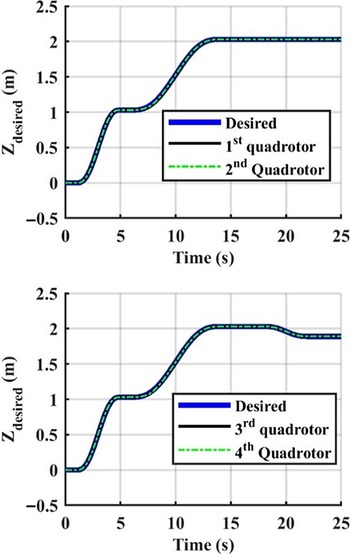
• The quadrotors raise to a height of 1.03 m. In this case, the ropes are not taut and the tensions of the ropes are zero. When quadrotors reach to the height of 1.03 m, the ropes are extended. The time allowed for this segment is 4 s, and the desired trajectory for this segment is as follows:
 \begin{align*} {z_{{q_{desired}}}} = \frac{{309{t^5}}}{{51,200}} - \frac{{309{t^4}}}{{5120}} + \frac{{103{t^3}}}{{640}}.\end{align*}
-
• Then, quadrotors lift the payload to a height of 1.03 m. The time allowed for this segment is 8 s, and the desired trajectory for this segment is as follows:
\begin{align*} {z_{{q_{desired}}}} = {{3{t^5}} \over {16,384}} - {{15{t^4}} \over {4096}} + {{5{t^3}} \over {256}} + 1.03.\end{align*}
-
• Finally, while the first and second quadrotors maintain their positions, third and fourth quadrotors decrease their height to reach to a height of 1.89 m. The time allowed for this segment is 4 s, and the desired trajectory is as follows
\begin{align*} {z_{{q_{desired}}}} = - \frac{{21{t^5}}}{{25,600}} + \frac{{21{t^4}}}{{2560}} - \frac{{7{t^3}}}{{320}} + 2.03.\end{align*}


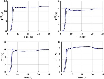
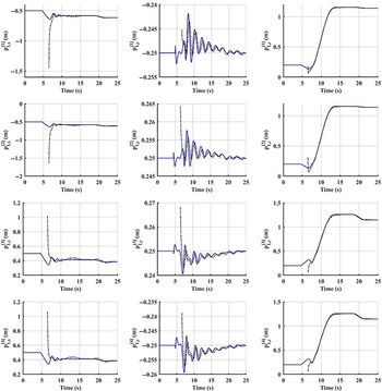
Time histories of each quadrotor to track the desired trajectory are shown in Fig. 2. It can be seen that the proposed position controller shows an acceptable performance and the effect of rope force is mainly compensated. Figure 3 shows the estimation of the force applied to each quadrotor. The blue-solid line is the applied force and the black-dashed line is the estimated force. This figure shows the satisfactory performance of the proposed adaptive controller.
Time histories of each quadrotor to track the desired trajectory.

Estimation of forces applied to each quadrotor.

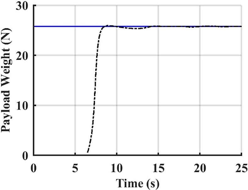
The estimation of the payload weight based on the previous estimation results is shown in Fig. 4. It can be seen that the estimated weight quickly converges to the actual value. As shown, the estimation has been started after 6 s, because before this time the ropes are not taut and there will be no estimation.
Estimation of the payload weight.

In comparison with the estimation algorithm presented in ref. [Reference Lee and Kim26], the proposed algorithm was found to be faster in response. The estimation time is almost 4 s in our algorithm compared with 30 s in ref. [Reference Lee and Kim26].
Figure 5 shows the appropriate estimation of attachment points in the inertial frame. Therefore, it can be said that the payload attitude is well known if the ropes are taut during the trajectory tracking.
Estimation of attachment points in inertial frame.

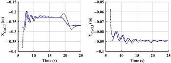
Figure 6 shows the estimation of CG positions in the inertial frame. As mentioned in Section 4, x and y CG positions can be estimated in the inertial frame, but the z component cannot be estimated. It can be seen that these two components were also estimated perfectly.
Estimation of CG positions in the inertia frame.

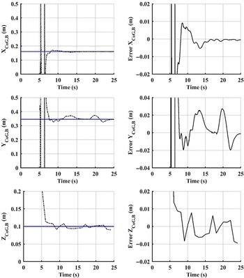
Figure 7 shows the estimation of CG positions in the body frame. It can be seen that the proposed algorithm provides an acceptable performance and the position errors for each component were found to be less than 2 cm. When the quadrotors held their positions, the position errors were obtained to be less than 1 cm.
Estimation of CG positions.

Finally, Fig. 8 shows the total thrust of each quadrotor. The distance between the CG and geometric center of the payload was calculated to be 17 cm, but the thrust of the quadrotor in vicinity of CG was almost twice of the farthest quadrotor. Apparently, the flight endurance is a function of this quadrotor. Thus, the positioning of quadrotors should be chosen such that the difference between the total thrust of quadrotors is minimized and consequently the flight endurance can be increased.
Total thrust of each quadrotor.

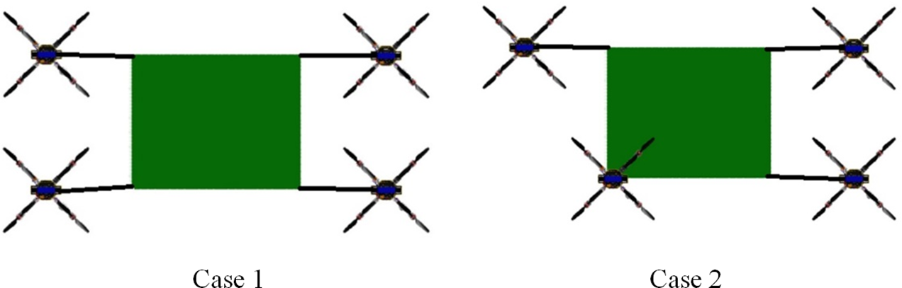
In order to show the significant effect of agents formation on flight endurance, two cases were considered for the formation flight: (1) all robots are at the same distance from the payload not considering the CG information, and (2) the position of the quadrotor in vicinity of CG was changed in order to make its connected rope vertical. Figure 9 shows the results of these two simulated cases.
Quadrotors formation in two cases.

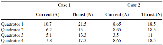
The current consumed by each quadrotor and its thrust force in both cases are also shown in Table I.
Currents consumed by each quadrotor and its thrust.

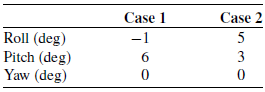
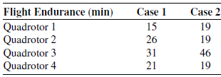
The payload attitude in these cases is shown in Table II. It was assumed that each quadrotor is equipped with a 2700 mAh battery cell. Therefore, the flight endurance of quadrotors was calculated in each case as listed in Table III.
Payload attitude in both cases.

Flight endurance for each quadrotor.

As it can be seen, the flight endurance is 15 min for case 1 and 19 min for case 2. Thus, the flight endurance has increased by 26%, and this was interestingly obtained by only changing the position of one quadrotor. Therefore, an optimal formation can be sought in future works according to the payload CG.
Finally, it can be inferred that quadrotors positions in a formation flight for load transportation should be determined considering the payload CG information, otherwise the system’s efficiency can be reduced greatly.
5.2. Transportation of a nonuniform rod by two quadrotors
The payload was modeled by a nonuniform rod with length = 1 m, where its position of the CG is 0.44 m as shown in Fig. 10. The parameters and reference trajectory used in the simulation were the same as in the previous example, except that the payload weight was considered 0.6 kg. The initial positions of two quadrotors were assumed to be
 $\xi _0^{\left[ 1 \right]} = \left[ {-1.5,0} \right]$
and
 $\xi _0^{\left[ 2 \right]} = \left[ {1.5,0} \right]$
.
Two quadrotors transporting a nonuniform rod; the payload is on the ground and the cables are not taut.

Figure 11 shows the final configuration of the payload and quadrotors. As it can be seen, due to the heterogeneity of the payload, it has an angle of 6° above the horizontal.
Final configuration of the payload and quadrotors.

Figure 12 shows the estimation of the force applied to each quadrotor. The blue-solid line is the applied force and the black-dashed line is the estimated force. This figure shows the satisfactory performance of the proposed adaptive controller.
Estimation of forces applied to each quadrotor.

The estimation of the payload weight is shown in Fig. 13. It can be seen that the estimated weight quickly converges to the actual value.
Estimation of the payload weight.

Finally, Figs. 14 and 15 show the estimations of CG position and rod angle. It can be seen that the proposed algorithm provides an acceptable performance in estimating the unknown parameters of the payload.
Estimation of CG.

Estimation of rod angle.

6. Conclusions
In this paper, the control of cooperative payload transportation using aerial robots has been presented. The unknown weight and the position of the CG payload were estimated using a parameter estimation algorithm. An adaptive controller was designed to estimate and compensate the force of the rope connected to each quadrotor. The simulation results for nonuniform rod and cubic payloads showed the successful tracking of the desired trajectory and also an excellent estimation of the unknown parameters. In the future work, the research will cover the development of an algorithm considering non-homogeneity of the payload and finding the best positions of the quadrotors based on decreasing difference of the total thrust of quadrotors to increase the flight endurance.
Conflicts of Interest
No potential conflict of interest was reported by the authors.
Appendix
The detail of
 $A_{3\left( {n + 1} \right) + 1}^{\left[ i \right]},A_{3\left( {n + 1} \right) + 2}^{\left[ i \right]},A_{3\left( {n + 1} \right) + 3}^{\left[ i \right]}$
and
 ${B^{\left[ i \right]}}\left( {q,\dot q} \right)$
used in Eqs. (12) and (13) can be written as follows:
 \begin{align*} \begin{matrix} {A_{3\left( {n + 1} \right) + 1}^{\left[ i \right]} = \left( {q_x^{\left[ i \right]} - p_x^{\left[ i \right]}} \right)} \\[4pt] {\left( {\left( { - {\rm{c}}{\phi _L}s{\theta _L}c{\psi _L} - s{\phi _L}s{\psi _L}} \right)p_y^{\left[ i \right]} + (s{\phi _L}s{\theta _L}c{\psi _L} - {\rm{c}}{\phi _L}s{\psi _L})p_z^{[i]}} \right)} \\[4pt] { + \left( {q_y^{\left[ i \right]} - p_y^{\left[ i \right]}} \right)} \\[4pt] {\left( {( - {\rm{c}}{\phi _L}s{\theta _L}s{\psi _L} + s{\phi _L}c{\psi _L})p_y^{[i]} + (s{\phi _L}s{\theta _L}s{\psi _L} + {\rm{c}}{\phi _L}c{\psi _L})p_z^{[i]}} \right)} \\[4pt] { + \left( {q_z^{\left[ i \right]} - p_{z,I}^{\left[ i \right]}} \right)\left( { - {\rm{c}}{\phi _L}c{\theta _L}p_{y,B}^{\left[ i \right]} + s{\phi _L}c{\theta _L}p_{z,B}^{\left[ i \right]}} \right)} \end{matrix} \end{align*}
 \begin{align*} A_{3(n + 1) + 2}^{[i]} = (q_x^{[i]} - p_{x,I}^{[i]})\left( s{\theta _L}c{\psi _L}p_{x,B}^{[i]} - s{\phi _L}c{\theta _L}c{\psi _L}p_{y,B}^{[i]} - {\rm{c}}{\phi _L}c{\theta _L}c{\psi _L}p_{z,B}^{[i]} \right) \\[4pt] { + (q_y^{[i]} - p_{y,I}^{[i]})\left( {s{\theta _L}s{\psi _L}p_{y,B}^{[i]} - s{\phi _L}c{\theta _L}s{\psi _L}p_{y,B}^{[i]} - c{\phi _L}c{\theta _L}s{\psi _L}p_{z,B}^{[i]}} \right)} \\[4pt] { + (q_z^{[i]} - p_{z,I}^{[i]})\left( {c{\theta _L}p_{x,B}^{[i]} + s{\phi _L}s{\theta _L}p_{y,B}^{[i]} + c{\phi _L}s{\theta _L}p_{z,B}^{[i]}} \right)} \end{align*}
 \begin{align*} A_{3\left( {n + 1} \right) + 3}^{\left[ i \right]} = \left( {q_x^{\left[ i \right]} - p_{x,I}^{\left[ i \right]}} \right)(c{\theta _L}s{\psi _L}p_{x,B}^{\left[ i \right]} + \left( {s{\phi _L}s{\theta _L}s{\psi _L} + {\rm{c}}{\phi _L}c{\psi _L}} \right)p_{y,B}^{\left[ i \right]}\end{align*}
 \begin{align*} + \left( {c{\phi _L}s{\theta _L}s{\psi _L} - s{\phi _L}c{\psi _L}} \right)p_{z,B}^{\left[ i \right]}) + \left( {q_y^{\left[ i \right]} - p_{y,I}^{\left[ i \right]}} \right)( - c{\theta _L}c{\psi _L}p_{x,B}^{\left[ i \right]} + \end{align*}
 \begin{align*} \left( { - s{\phi _L}s{\theta _L}c{\psi _L} + {\rm{c}}{\phi _L}s{\psi _L}} \right)p_{y,B}^{\left[ i \right]} - \left( {c{\phi _L}s{\theta _L}c{\psi _L} + s{\phi _L}s{\psi _L}} \right)p_{z,B}^{\left[ i \right]})\end{align*}
 \begin{align*} {{\rm{B}}^{\left[ i \right]}} = - (\dot q_x^{\left[ i \right]} - \dot p_x^L - \left( { - {{\dot \theta }_L}s{\theta _L}c{\psi _L} - {{\dot \psi }_L}c{\theta _L}s{\psi _L}} \right)p_{x,B}^{\left[ i \right]}\end{align*}
 \begin{align*} - \left( {{{\dot \phi }_L}\left( {{\rm{c}}{\phi _L}s{\theta _L}c{\psi _L} + s{\phi _L}s{\psi _L}} \right) + {{\dot \theta }_L}s{\phi _L}c{\theta _L}c{\psi _L} - {{\dot \psi }_L}\left( {s{\phi _L}s{\theta _L}s{\psi _L} + {\rm{c}}{\phi _L}c{\psi _L}} \right)} \right)p_{y,B}^{\left[ i \right]}\end{align*}
 \begin{align*} - \left( { - {{\dot \phi }_L}\left( {s{\phi _L}s{\theta _L}c{\psi _L} - c{\phi _L}s{\psi _L}} \right) + {{\dot \theta }_L}c{\phi _L}c{\theta _L}c{\psi _L} - {{\dot \psi }_L}\left( {c{\phi _L}s{\theta _L}s{\psi _L} - s{\phi _L}c{\psi _L}} \right)} \right)p_{z,B}^{\left[ i \right]}{)^2}\end{align*}
 \begin{align*} - (\dot q_y^{\left[ i \right]} - \dot p_y^L - \left( { - {{\dot \theta }_L}s{\theta _L}s{\psi _L} + {{\dot \psi }_L}c{\theta _L}c{\psi _L}} \right)p_{x,B}^{\left[ i \right]}\end{align*}
 \begin{align*} - \left( {{{\dot \phi }_L}\left( {{\rm{c}}{\phi _L}s{\theta _L}s{\psi _L} - s{\phi _L}c{\psi _L}} \right) + {{\dot \theta }_L}s{\phi _L}c{\theta _L}s{\psi _L} + {{\dot \psi }_L}\left( {s{\phi _L}s{\theta _L}c{\psi _L} - {\rm{c}}{\phi _L}s{\psi _L}} \right)} \right)p_{y,B}^{\left[ i \right]}\end{align*}
 \begin{align*} - \left( { - {{\dot \phi }_L}\left( {s{\phi _L}s{\theta _L}s{\psi _L} + c{\phi _L}c{\psi _L}} \right) + {{\dot \theta }_L}c{\phi _L}c{\theta _L}s{\psi _L} + {{\dot \psi }_L}\left( {c{\phi _L}s{\theta _L}c{\psi _L} + s{\phi _L}s{\psi _L}} \right)} \right)p_{z,B}^{\left[ i \right]}{)^2}\end{align*}
 \begin{align*} - {\left( {\dot q_z^{\left[ i \right]} - \dot p_z^L + {{\dot \theta }_L}c{\theta _L}p_{x,B}^{\left[ i \right]} - \left( {{{\dot \phi }_L}{\rm{c}}{\phi _L}c{\theta _L} - {{\dot \theta }_L}s{\phi _L}s{\theta _L}} \right)p_{y,B}^{\left[ i \right]} + \left( {{{\dot \phi }_L}s{\phi _L}c{\theta _L} + {{\dot \theta }_L}c{\phi _L}s{\theta _L}} \right)p_{z,B}^{\left[ i \right]}} \right)^2}.\end{align*}