

1. Introduction
One important insight from historical analysis of market integration is that long-distance trade often takes place out of the (trade-cost adjusted) law of one price equilibrium. That is, the law of one price is violated, which will affect the volume of trade relative to its equilibrium value. We hypothesize that a major source of violations of the law of one price was unreliable and slowly travelling information over long distances and the difficulties for the wider public in getting access to price data. The motivation for this hypothesis is that the time in transit of commodities does not change dramatically in the period we are examining and inventories exist at both ends of the transport chain.Footnote 1 Adjustments in inventories will react to new information immediately. The information traders in Chicago had on prices in Liverpool was about two weeks old (and vice versa) before the Atlantic cable came into operation in the 1860s. The introduction of the transatlantic telegraph shortened the transmission time to a few hours. With the telegraph the speed at which information travelled became dramatically shorter than the speed of transporting goods for the first time in history.
However, costs of telegraphic transmission were high initially and information might be kept private by merchant houses. A flourishing commercial press turned what used to be exclusively or privately held knowledge into publicly accessible information in the 1870s, when price data from the market day preceding the date of publication were routinely published and presented as transmitted by ‘cable’. Traders in Liverpool or London were therefore well informed about prices in, say, Chicago, New York, Odessa, Paris and vice versa with about one working day's delay. While the larger merchants' houses had access to telegraph transmission directly, others relied on ‘cable news’ reported in the press. However, we do not have continuous price data to test whether information technology changes caused structural breaks in the price adjustment.
Persson (Reference Persson1999) and Ejrnæs and Persson (Reference Ejrnæs and Persson2000) showed that over the last five centuries market performance improved gradually as measured by the speed at which deviations are reversed or corrected. The half-life of shocks to the law of one price in long-distance trade declined between 1500 and 1900 from years to days. The process of improved market efficiency gained momentum in the nineteenth century with faster and more reliable means of information transmission. In Section 6 we will assess the importance of improved information transmission relative to other plausible explanations.
The principal new problems addressed in this article, having first demonstrated the existence of a (trade-cost adjusted) law of one price equilibrium, henceforward LOOP, are:
1. to measure the welfare losses of imperfect market integration, that is the economic costs in terms of trade forgone as well as the deadweight loss when LOOP is violated;
2. to document the improvements in market efficiency and to estimate the gains thereof over time focusing on two periods, one before and one after the transatlantic telegraph.
An accounting framework for measuring trade forgone in disequilibrium is developed and, by implication, we assess the gains from improved market efficiency. For reasons that will be explained in Section 3, the word trade is used as a synonym for contract. The trade forgone is defined as the shortfall of traded (contracted) quantities when LOOP is violated from trade in the LOOP equilibrium. The intuition of the proposed framework is simple. We first determine the traded or contracted volume in the law of one price equilibrium at a major consumer and import market, Liverpool, which is supplied by a major export market, Chicago. If the price in Liverpool rises above the law of one price equilibrium, then actual transactions, i.e. the quantities contracted, will be lower than in equilibrium since demand is smaller than in equilibrium (assuming a negatively sloped demand curve). Quantities traded are constrained by demand. If the price in Liverpool falls below the equilibrium price, then transactions will be constrained by a smaller supply than in equilibrium, given an upward-sloping supply curve. The forgone trade in the tâtonnement process is the loss in terms of contracts forgone, that is the sum of the difference over an extended period of trading sessions between the law of one price equilibrium trade and quantities actually traded during the tâtonnement process. We do not have information on actual quantities, but, by specifying demand and supply elasticities, we can determine an equilibrium. The forgone trade will be estimated as a proportion of the equilibrium trade. The concept of forgone trade is akin to the concept of deadweight loss, as explained and discussed in Section 4. We focus on deadweight loss because it is widely used as a yardstick for efficiency gains and because deadweight losses are routinely dismissed as too small to matter much. We will challenge conventional wisdom. A limitation of the analysis followed here is that we portray the world trading system as a bilateral case. We are therefore cautious in drawing strong conclusions as to the effect on world trade in wheat from the results. However, it turns out that price movements, say in Liverpool, were fairly uniform on all types of wheat, domestic as well as foreign. Price levels differed according to origin and quality, but changes were similar in direction and magnitude. The same pattern emerges for the US market. Major market exchanges in the US had well-synchronized price movements. It is plausible that the conclusions regarding improved market efficiency that we reach are valid for most long-distance trade relations and Britain became, over time, increasingly dependent on transoceanic wheat supplies.
We analyse wheat in two major markets, exports from Chicago to Liverpool, and over two periods: one pre-telegraph period, 1858–62, when grain trade was lively a decade after the repeal of the British Corn Laws; and one period, 1883–9, when trade had stabilized at a high level. The latter period had access to telegraphic transmission and a specialized commercial press. The price data used in this study are collected from the contemporary press; see Appendix 1. We expect a major shift in market efficiency between the periods, which is linked both to the expansion of trade and traders and because the two periods were characterized by radically different information ‘regimes’. It can be safely assumed that the efficiency of a market is linked to access to information as long as there are no serious obstacles to entry into the trade. The choice of periods is imposed by the availability of price and transport cost data. It would have been desirable to cover the actual period when the transatlantic telegraph was introduced, but that is a period when the export of US grain ceased temporarily. Other important export markets, such as Russia, would have been interesting to study, but we have not been able to trace sufficiently reliable data to do this (see, however, Goodwin and Grennes Reference Goodwin and Grennes1998).
The article is organized as follows. In Section 2, the nature of the law of one price equilibrium is analysed in an error correction model. Section 3 motivates and formalizes the notion of excess demand and excess supply. In Section 4, the costs of imperfect market integration are assessed. Section 5 presents a counterfactual assessment of trade forgone over an extended period. Section 6 confronts the hypothesis that improvements in market efficiency were driven by faster and more reliable information with other explanations, and Section 7 concludes. The data are described in Appendix 1.Footnote 2
2. The nature of the law of one price equilibrium
In this section we derive the definition of the law of one price, where we explicitly take into account the presence of transport and transaction costs. Let PL and PC denote the prices in Liverpool and Chicago respectively. Furthermore, we also observe the transport cost, PTc. All prices are measured in the same currency and units, shillings per imperial quarter.
The law of one price adjusted for trade costs (LOOP) implies the following equilibrium:

where δ measures other, that is non-observed, transaction costs, for example commissions and insurance fees. This term can also reveal a high risk premium as well as quality differentials, as revealed by price differences between the grades of wheat if they differ between the export and import markets. This term is assumed to be constant during each of the two periods, but might differ between the periods. It is assumed to be proportional to the price in Chicago plus transport costs. Deviations from the LOOP equilibrium can be expressed in terms of differences in the logarithm of the prices:

On the basis of deviations from the equilibrium, the error correction model can be derived.
Error correction modelling of spatial price adjustments is based on the insight that equilibrium is an attractor with varying degrees of power rather than a state in which economies rest. Strictly speaking, the equilibrium price is rarely obtained and when observed it often does not last many trading sessions. Adjustments back to equilibrium take time and new stochastic shocks appear frequently. The fact that the adjustment after a shock is not instantaneous implies that markets are not in equilibrium during the adjustment (i.e. tâtonnement) process and trade will be constrained (relative to equilibrium levels) either by insufficient demand or insufficient supply.
The intuition behind the error correction model is that prices in Liverpool and Chicago will react if there is a deviation from equilibrium. In this case, the prices will adjust such that the deviation from equilibrium is decreasing. The error correction model is usually expressed in differences of log prices. Let ΔpLt = ln PLt − ln PL t − 1 and ΔpCt = ln PCt − ln PC t − 1. The error correction model in this version is given by:
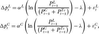
where λ = ln (1 + δ) ≈ δ and ϵCt and ϵLt are error terms with are assumed to be normally distributed with mean zero and constant variances:
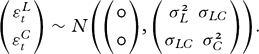
The parameters of the model can be estimated using maximum likelihood techniques. This model is a special case of the general error correction model where the equilibrium relation is assumed known.Footnote 3 The expected sign of the αL parameter is negative and it is positive for αC.
2.1. The estimation results
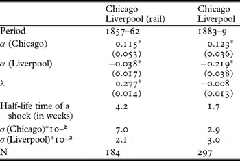
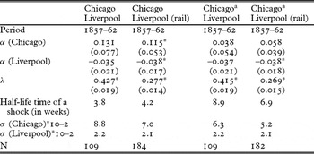
The model outlined above is estimated on the basis of weekly reported wheat prices in Liverpool and Chicago (for further details about the data, see Appendix 1). Table 1 above reports the results which strongly support the expectation of improved efficiency in Chicago to Liverpool trade. There is a marked decline in the half-life of shocks from 4.2 to 1.7 weeks. While most of the adjustments occurred in Chicago in the early period, Liverpool took most of the adjustment in the later period.Footnote 4 However, adjustments were mutual, which indicates the absence of ‘market dominance’ in both periods and the parameters have the expected signs. Results differ a little but not significantly depending on whether we use transport cost data for ships over the Great Lakes or rail all the way to New York for shipment to Liverpool. Tests for unit roots are in Appendix 2 and sensitivity analyses are reported in Appendix 3.
Estimates from the error correction model applied to Chicago and Liverpool trade in wheat

λ is significant and positive in the first period. In fact it is much too large to indicate unobserved costs only. There are two additional reasons for the magnitude of λ. First, market imperfections might cause excess profits or the nature of trade might demand a high-risk premium. Elsewhere we have been able to document a gradual decline in the unexplained residual price gap between the US and UK markets after the introduction of the telegraph (Ejrnæs, Persson and Rich Reference Ejrnæs, Persson and Rich2008). Second, the high value of λ has also to do with the fact that the quality quoted in Chicago (spring no. 2) is inferior relative to the quality quoted in the importing market (American white). In an efficient market, and if all transport and transaction costs are observable and recorded, λ should be zero, which it to say that the equilibrium price differences between markets are due only to transport and transaction costs. This is also the result that we have obtained for the later period. However, a word of caution is necessary here. The insurance cost, around 1 to 2 per cent of the value of the cargo, is (probably) not included in the price and transport cost data we use, and if so, λ should take a positive value but close to zero. The explanation for this not being the case has to do with the fact that the grade quoted in Liverpool for most of the period was for a slightly wider denomination: in terms of grades it contains spring no. 2 and inferior spring wheat, compared to Chicago for which we quote spring no. 2 alone (see Appendix 1). The data do not suggest significant changes in the quality differential over the relatively short periods under consideration in this study. That said, the λ for the second period indicates that the market was efficient. Furthermore, variance in price shocks falls sharply for the exporting market down to the level of the importing market.Footnote 5
3. A model of excess demand and supply
An important insight from historical market integration studies is that the law of one price equilibrium is rarely obtained as a stable state. It should rather be seen as an ‘attractor equilibrium’, that is a state to which the price reverses after a shock to equilibrium or in an ongoing reversal process. This view also relies on a realistic view of the tâtonnement process. It is not one in which sellers and buyers exchange trade bids and counter-bids before they reach an equilibrium price at which they trade. The tâtonnement process here is one observed in actual markets where trade takes place, albeit on a constrained level. Either buyers chase sellers, who ration the supply – a case of excess demand which will push prices up – or sellers chase buyers, who ration their purchases – a case of excess supply, in which prices are traded down. The contemporary commercial press, from which the price and transport cost data used in this study were collected, give ample evidence of trade taking place during the tâtonnement process. The press repeatedly reported periods of excess supply and in a sequence of trading sessions you can actually trace the tâtonnement process when sellers chase buyers, eventually giving in so that prices gradually fall in subsequent trading sessions. The press and business journals recorded prices and the state of the market as ‘quiet’ or ‘busy’, ‘dull’ or ‘lively’, indicating not only the volume but also the ‘mood’ of trade. For example, trade was often recorded as limited due to expected changes in price. It is clear that trade was actually taking place because occasionally the price was characterized as ‘nominal’, indicating that a session was not associated with trade at all but prices were just repeated from the preceding session. In the tâtonnement process the volume of trade could be reported as below normal, that is equilibrium, trade.
The quantities contracted on a particular market day will not necessarily equal the imports that day or the orders to Chicago for shipments because there are speculative inventory adjustments. For example, when prices rise above equilibrium sellers might mistake that for a permanent rise and increase their imports. However, given that the actual contracts sold will be constrained by the reduced demand at an above equilibrium price, inventories will build up and reduce imports at some future date when inventory levels will be reduced. When the price in Liverpool is below the equilibrium price traders might wait until the price in Chicago falls until they place orders, and in the meantime they will reduce inventories. Over an extended period of trading sessions, say, a couple of years, the contracted volumes will be (approximately) equal to the actual imports in that extended period. The reason is that the difference in the volume of inventories between the initial trading session and the final market day of the trading period will be very small relative to the sum of the contracted volumes during the entire period. This view amounts to maintaining that inventory adjustments are a stationary process, and no more is needed for our argument. The fact that price adjustments became much faster than the pace of shipments of commodities was related to inventory adjustments triggered off by the increasingly swift transmission of information. When information about supply increases in Chicago reached Liverpool, prices began falling immediately in Liverpool because grain was sold from the warehouses. On both sides of the Atlantic there were warehouses to store grain. The storage facility is a necessity given the fact that grain is produced once a year but consumed over the entire period. Since harvest time was usually associated with lower prices, a substantial storage capacity was essential for successful speculative behaviour. An additional factor which probably helped to generate fast tâtonnement was an emerging trade including grain on passage, so called ‘floating cargo’ trade. This was, however, a phenomenon of minor importance in the first period we investigate in this article. As noted below we have not been able to substantiate a conjecture implied by Coleman (Reference Coleman2009) that a fall in the frequency of stock-outs might contribute to the smaller violations of the law of one price.
Let us now turn to a formal framework for calculating the loss to contracted volumes due to excess supply and demand as described above.
We assume that the demand curve in Liverpool is given by

where QDt is the demand for American wheat in Liverpool and PLt is the price of American wheat. ρ1 is the price-elasticity of demand (ρ1 < 0). The supply of American wheat for the English markets is determined by the following supply function:

where QSt is the supply of American wheat for Liverpool, PCt is the price of American wheat in Chicago. τ1 is the price elasticity of supply (τ1 > 0).
In equilibrium the price in Liverpool will be equal to the price in Chicago adjusted for transaction costs

PTct is the transport cost from Chicago to Liverpool and Δ measures additional transaction costs (such as port and porter charges, commissions and insurance), which are assumed to be proportional to the price in Chicago plus transport costs. The quantity obtained at the equilibrium price is denoted ln Qeqt

If the price in Liverpool exceeds the trade cost corrected price in Chicago PLt > (PCt + PTct)(1 + δ) we will observe excess supply of wheat in Liverpool and the contracted volumes will fall. The fall is

If the changes are small the left-hand side of the equation above can be interpreted as the percentage fall in the contracted quantity.
On the other hand, if the price in Liverpool falls below the trade cost corrected price in Chicago PLt < (PCt + PTct)(1 + δ) we will observe excess demand of wheat traded in Liverpool and the actual volume of contracts will fall. That fall compared to equilibrium contracting can be expressed by

From the two equations for the fall in quantity, the key aspect is the deviation between the prices in Liverpool and in Chicago (corrected for transaction costs). In the following section we will investigate the extent of price deviations and the implied effects on trade.
4. Estimating the costs of imperfect market integration
In order to estimate the cost of imperfect market integration we will need some estimates of supply and demand elasticities. What are the likely elasticities of demand and supply? There have been a number of attempts to estimate UK and US elasticities of demand and supply (Irwin Reference Irwin1998; Williamson Reference Williamson1980, Reference Williamson1990; Olson and Harris Reference Olson and Harris1959), and on that basis demand elasticity is estimated to be in the range of 0.5–1 and US export supply elasticity to be between 0.5 and 1.5. While there is evidence that demand for food in general is inelastic, it could be argued that US wheat is a special case since it was a prime export quality – it sold at a premium of 5 to 10 per cent relative to domestic wheat in Britain, and for that reason elasticities might be higher than for food or wheat in general.
Given estimates of demand and supply elasticities, we can calculate the average fall in trade compared to the equilibrium. In the short run the actual import trade of US wheat might differ from the contracts sold for immediate and quasi-immediate delivery. However, as explained in Section 3, imported and contracted volumes will be approximately equal over an extended period since inventory adjustments between the initial market session and the last will be small relative to the traded and imported volumes. For that reason we will henceforward use the word ‘trade’ as synonymous with ‘contracted volume’. The average forgone trade is calculated as:

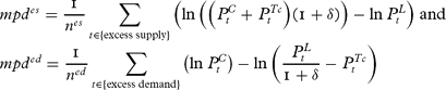
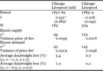
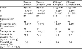
where nesand ned are the number of trading sessions with excess supply and demand respectively and mpdes and mpded are the mean price deviations when we have excess supply and demand.Footnote 6 We display the estimates of the average loss in trade in Table 2 for two pairs of values of the elasticities.
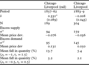
Estimating the forgone trade due to imperfect market integration

Table 2 provides an upper- and lower-bound estimate of the trade forgone due to deviations from LOOP trade. The inefficiency of the pre-telegraph transatlantic trade is apparent. It reduces equilibrium trade by as much as 13 per cent in the upper-bound estimate and close to 5 per cent in the lower-bound estimate. The gain from improved market efficiency is the difference in the mean fall in traded quantity between the two periods. The first conclusion is that the gains from increased market efficiency between the first and second periods are substantial in the upper-bound estimate and clearly non-trivial in the lower-bound estimate. In the upper-bound estimate the gain is 8.3 per cent of equilibrium trade (13.7 − 5.4 = 8.3) and in the lower-bound estimate it is 3.1 per cent (5.2 − 2.1).
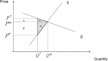
We also calculate the deadweight loss associated with imperfect market efficiency for the two periods. When the price P* exceeds the equilibrium price, Peq we are in a situation of excess supply since traders in Chicago are willing to sell more than the equilibrium quantity. The price axis in Figure 1 shows the price in Liverpool, which implies that the supply schedule S is the price in Chicago plus the cost of transport to Liverpool.
The deadweight loss in a period of excess supply

The area A + C is the consumer surplus and B + D is the producer surplus. However, at P* the consumer surplus A will be transferred to the producer, given the above equilibrium price. The deadweight loss is therefore the triangle C + D. When price is below equilibrium at, say, P** there is a reduction in producer surplus equal to the area B + D in Figure 1, but B is transferred to consumers because of the below equilibrium price. Again the deadweight loss will be C + D. We calculate the deadweight loss relative to value of the traded quantity in equilibrium (see Appendix 4 for details):

Similarly, we can calculate the relative deadweight loss when the price, P*, falls below the equilibrium price (excess demand):

Based on these two expressions we can calculate the average deadweight loss for the two periods.
The results reported in Table 3 show that the deadweight loss is between 3.4 per cent of equilibrium trade in the upper-bound estimate and 1 per cent in the lower-bound estimate in the period 1857–62, while it falls to between 0.5 to 0.2 per cent in the period 1883–9. Again we see a considerable fall in the deadweight loss due to improved market efficiency and the loss is so small that markets can be considered efficient.
Estimating the average relative deadweight loss due to imperfect market integration

5. A counterfactual
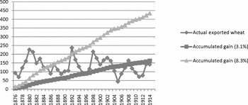
In this section we present two different ways of assessing the importance of the gains in trade from the improved market efficiency. First, we design a counterfactual scenario. The actual trade is the observed value of yearly wheat exports from the USA between 1875 and 1914 measured in current US dollars. The year 1875 is chosen as the starting year of the modern information regime, permitting a fairly efficient spatial arbitrage. Export of grain in the 1875 to 1914 period is considered to represent trade at the market efficiency characteristics reported in Table 2 for the 1883–9 period. Imagine now that no improvement in market efficiency took place after the 1858–62 period, which would be a likely scenario had the transatlantic telegraph not been introduced. Then trade would have been smaller than the actual trade since there were significant improvements in market efficiency between the first and second period documented in Table 2. Had market efficiency remained at the 1858–62 level we can calculate counterfactual trade to be 3.1 per cent lower than actual trade each year in the 1875–1914 period in the lower-bound estimate and to be 8.3 per cent lower per year in the upper-bound estimate. The gain from improved market efficiency is the difference between trade at the 1883–9 efficiency level, which is assumed to be the efficiency level of the entire 1875–1914 period in this counterfactual estimate, and the efficiency level of the 1858–62 period. The counterfactual question then is: what will the accumulated gains from improved market efficiency be like? In Figure 2 below we present the upper-bound and lower-bound estimates. The argument is made under the assumption that the Chicago to Liverpool trade was typical enough to permit a generalization to US wheat exports. Given the fact that the UK was the major market and London and Liverpool the dominating commodity exchanges in Britain, that assumption is not unreasonable.
Actual US wheat exports and accumulated gains from improved market efficiency, 1875–1914, in a lower-bound and upper-bound estimate of market efficiency gains (millions of US dollars)
Source: Mitchell Reference Mitchell1993, table E3.

Figure 2 indicates that the accumulated gains from improved market efficiency in the upper-bound estimates are equivalent to about four and a half years of average wheat exports in the period or to one and a half years of average exports using the lower-bound estimate.
Second, we compare the gain in efficiency to the gain from reduced transport costs. In the literature on market integration the transatlantic freight rate decline has been a major factor stimulating trade. It is possible to compare the gains from increased market efficiency with the decline in transport costs You can view transport costs as a tax or fee accruing to the transport sector and thereby estimate the deadweight loss of transport costs. That makes the reduction in the deadweight loss from improved market efficiency comparable to the reduction in deadweight loss from falling transport costs. Recent estimates of the fall in the transatlantic freight factor for wheat show that it fell by approximately 3.5 percentage points between 1850 and 1900, from ca. 10.5 to 7 per cent (Persson Reference Persson2004). Almost all of that decline took place between 1875 and 1895. The deadweight loss associated with transportation cost of 10.5 percentage points can be calculated in a similar way and is found to be between 0.6 and 0.9 per cent of the value of the traded quantity. When the transport cost falls to 7 per cent, the deadweight loss is reduced to 0.2–0.4 per cent. We can easily see that the gain in deadweight loss from reduced transport cost is substantially smaller than the gain from improved market efficiency in approximately the same period.
6. What caused the improvement in market efficiency?
We have advanced the hypothesis that the improvement in market efficiency was caused by the observed regime change in information transmission, which initially triggered off price adjustments via inventory changes. But it is necessary to consider other potential causes. To do so we need to decompose the improvement in market efficiency.
Roughly speaking, there are three components of about equal importance: a fall in the variance of shocks to the price processes; faster adjustment of prices after shocks to the equilibrium price; and a decline in the unexplained price difference between markets, that is the residual difference not explained by observed trading costs.
We admit that the decline in variance might have been influenced by the introduction of future markets between the first and second periods. It has been argued that market integration in itself can be expected to suppress variance in local markets because the variance of local harvest outcomes is larger than in global harvests (Persson Reference Persson1999). The speed at which information about global events enters will therefore reduce the impact of local shocks. However, there is little reason to believe that future markets in, say, Chicago should impact upon the residual price difference or adjustment speed between markets. Much of the change in adjustment speed is driven by Liverpool adjusting faster to shocks in Chicago, and it is plausible that a fast flow of news will be the major factor given the fact that Liverpool had a lively floating cargo trade and opportunities for inventory adjustment. However, the introduction of the gold standard muted exchange rate risks, which might have contributed to the fall in the residual price difference if we interpret it as a risk premium.
It can also be argued that faster and more reliable information reduced risk. To the extent that residual price differences were caused by traders having access to private information, then the commercial press which routinely reported ‘cable’ news effectively reduced excess profits from insider trading. We noted in Section 2 that some part of the residual price difference might be due to quality differences between the wheat, which makes it risky to draw too strong conclusions.
What role, if any, do particular institutional or political factors have in the observed change in market performance? The first period we study partly coincides with the outbreak of the American Civil War. Jacks (Reference Jacks2005) argues that the outbreak of the war increased trade costs and might have made otherwise well-functioning markets perform less well, and in particular increased price volatility in the first period. However, increased trade costs do not necessarily increase the residual, or unexplained, price-differential between markets. Nor do they plausibly contribute to a slowdown in the adjustment speed. Besides, we have not observed unusually large shocks in trade costs, although there are a small number of spikes in 1861 which might be related to the war. It turns out that the major results remain if these observations are removed; see Appendix 3.
In a recent article, Coleman (Reference Coleman2009) has shown that constraints in storage can cause violations of the law of one price. For example, an adverse output shock in a market might bring inventory levels down to zero, and prices will then depart from the law of one price until new shipments arrive. However, we do not have time series over volumes in warehouses to see whether, over time, stock-outs, that is extremely low inventory levels, became less frequent. If they did, this could be a contributing factor to an increase in market efficiency. Evidence from The Economist's weekly corn trade report does not support the view that stock-outs were frequent in either period in our investigation. We have looked at all the outliers in the data and the most frequent single cause was (rumours of) political and or military conflict. Second comes meteorological news and in only one case were we able to trace the outlier as caused by storage failures.
In conclusion, the introduction of the telegraph and an accompanying commercial press seems to be the most important although not the sole cause in reducing residual price differences and the increase in the speed of adjustment between markets.
7. Conclusion
In recent years, a number of studies have documented the increased efficiency in long-distance market integration. However, this article brings a number of novel insights about the welfare implications of improved market performance.
The LOOP was alive and kicking in the nineteenth-century international economy. Adjustment speed as measured by the half-life of shocks to LOOP was not a matter of years or months but weeks, and it fell over time. That result underlines the need for high-frequency data in historical PPP studies.
A method by which the costs of disequilibrium trade and, by implication, the gains from improved market efficiency can be measured has been developed. Gains are substantial in an upper-bound estimate and significant in a lower-bound estimate. Deadweight losses, or more popularly Harberger triangles, are routinely dismissed as too small to be bothered about in historical analysis. That is the guiding principle, albeit made in another context, by D. McCloskey in analysing productivity gains in the British Industrial Revolution (McCloskey Reference Mccloskey, Floud and McCloskey1994, see especially pp. 259–70). We disagree and we have shown that there is a need to challenge the conventional wisdom. The relative deadweight loss as reported in Table 3 is between 1 and 3.4 per cent of trade in the first period and falls considerably, so that markets in the post-telegraph nineteenth century can be considered to have experienced a regime change towards more efficient markets. Market efficiency increases over time, but there seems to be a regime shift caused by changes in the information technology associated with the telegraph and the development of the business press. But are these gains big or small? It depends on the standard used. The impact of improvements in market efficiency compares well and even outpaces falling transport costs, which is the factor normally ascribed a leading role in nineteenth-century trade expansion.
Acknowledgements
We would like to thank two anonymous referees, the Editors, Carl-Johan Dalgaard, Markus Lampe and Paul Sharp for useful suggestions. One of the authors acknowledges support from the Danish Social Science Foundation.
Appendix 1: Description of the data
Prices refer to spot transactions on the first market day every week, usually Monday (Tuesdays in Liverpool) and have been converted to shillings per imperial quarter.
Period 1858–62: prices of spring no. 2 in Chicago are from Trade and Commerce of Chicago, Chicago Board of Trade Annual report, and refer to spring no. 2 except January to 12 June 1858, when unspecified spring. The new grading system is introduced in 1858. Prices in Liverpool from Liverpool Journal and Liverpool Courier and refer to American white. Transport costs between Chicago and New York from Chicago Board of Trade, Annual report. Transport costs between New York and Liverpool from New York Times.
Period 1883–9: transport costs and prices in Chicago and Liverpool are from the Annual Report of Chicago Board of Trade. Prices refer to spring no. 2 in Chicago and fair-to-good spring wheat (US) in Liverpool from 1883 to 1886 and from 1887, spring no. 2.
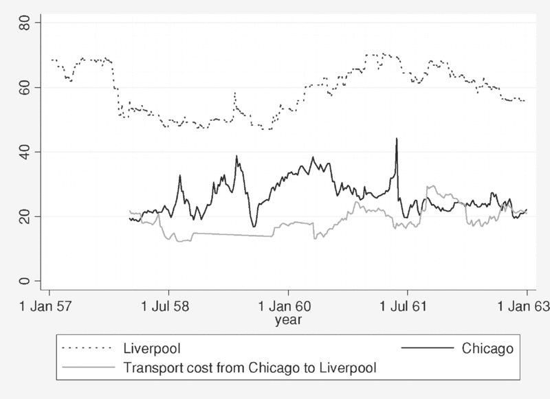
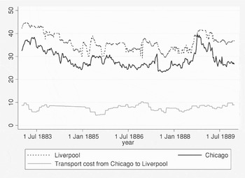
Exchange rates refer to three months' bills of exchange collected by J. Schneider et al. (eds.), Währungen der Welt I, Europäische und Nordamerikanische Devisenkurse, 1777–1914, vol. 1 (Stuttgart: Franz Steiner Verlag, 1991). The prices are shown in Figures A1 and A2.
The weekly wheat prices in Liverpool and Chicago, 1857–62 (shillings per imperial quarter)
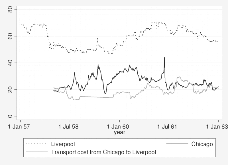
The weekly wheat prices in Liverpool and Chicago, 1883–9 (shillings per imperial quarter)

Appendix 2: Test for unit root
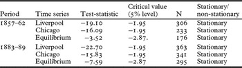
Estimation of the error correction model relies on the assumption that the time series Δln PLt, Δln PCt and ln (PLt) − ln (PCt + PTct) are stationary processes. To examine if this is the case the Dickey-Fuller test for a unit root (non-stationarity) is performed. The results of the test are reported in Table A1.
Dickey-Fuller test for unit root

Appendix 3: Sensitivity analyses
The price data for Chicago have one extreme observation, 13 May 1861. We have performed the analyses with and without this observation. Furthermore, we have also used transportation costs based on rail freight rates to New York as well as the Great Lakes plus canal to New York.
Both adjustment speed and variance are affected by the extreme observation but in opposite directions, which means that our estimate of the trade forgone by inefficient markets, which depends on adjustment speed and variance, is only marginally affected, as is revealed by Table A3.
Estimation results from the error correction model

aThe observation for 13 May 1861 is excluded.
Estimating the forgone trade due to imperfect market integration

aThe observation for 13 May 1861 is excluded.
Appendix 4: Deadweight loss
The relative deadweight loss is defined as

If P* /Peq, P** /Peq and Q* /Qeq are close to one, which means that we have relatively small price deviations from the equilibrium price we can use the following approximation: ln(e + 1) = e where e close to zero

By using the supply and demand function we get

Inserting these expressions in the equation for deadweight loss we get