Basic antenna structure

The structural configuration of the proposed antenna is shown in Figure 1. Fabricated via standard PCB etching technology, the antenna employs a 0.035 mm-thick copper radiator and a 1.6 mm-thick FR4 substrate with a dielectric constant of 4.4. This design incorporates a magnetic loop structure. The tag chip is placed at the center of the loop’s feed line. The distance from the chip to each end patch is L1. Slots with dimensions length (a) and width (b) are cut into two end patches. Asymmetric dipole structures are positioned on both sides of the feed line, with their dimensions defined by L2, W2 and L3, W3. The length and width of these dipole arms decides the antenna’s impedance matching. The RFID IC matched with the antenna in this design is UCODE 8, bonded across a narrow gap. The microchip has a read sensitivity of $-$21.85 dBm and an impedance of 13–j191 $\Omega$ at 916 MHz.

Figure 1.

Structure of tag antenna. (a) Tag antenna structure configuration. (b) Prototype physical image.

Figure 1 Long description

The image A showing a dimensioned layout drawing and an exploded view of a tag antenna. The top drawing shows a rectangular antenna outline with a dimension line labeled L along the bottom edge and a dimension line labeled W along the left edge. Inside the outline, two long rectangular patches contain repeated narrow rectangular slots arranged in a row, one patch near the top and one patch near the bottom. A central horizontal feed line runs between the two slotted patches and the text UCODE 8 IC chip is placed on this central line. Dimension callouts labeled L1, L2, L3, W2 and W3 appear around the internal features and the slot dimensions are labeled length left parenthesis a right parenthesis and width left parenthesis b right parenthesis. Below, an exploded view shows layered rectangular sheets separated by gaps, with arrows pointing to labels Substrate, Chip and Stub. The image B showing a photo of the fabricated antenna on a rectangular board, with three arrow labels pointing to features named Dipole patch, Chip slot and Stub.

We design and optimize the tag antenna, and study its input impedance, radiation efficiency, and gain in Ansys HFSS. The design dimensions are summarized in Table 1.

Table 1.

Dimensions of the antenna

Table 1 Long description

The table lists antenna geometric parameters and their dimensions in millimeters. The largest dimension is L at 64 mm, followed by overall width W at 42 mm. The height H is 1.6 mm, indicating a thin structure relative to its length and width. Mid-sized lengths include L1 = 15 mm, L3 = 11.2 mm, and L2 = 9.6 mm. Smaller width features are W1 = 1 mm, W2 = 1.5 mm, and W3 = 1.7 mm. Additional parameters are a = 16 mm and b = 7 mm, while spacings s1 and s2 are both 4 mm. The smallest listed values are d1 and d2 at 0.2 mm each. Values are provided as named parameters without definitions, so interpretation depends on the antenna drawing or design notes.

Although the overall layout may appear relatively large compared with some compact RFID tags, its physical dimensions correspond to $0.1951\lambda \times0.128\lambda\times0.0051\lambda$ at 915 MHz. From an electrical perspective, the antenna remains electrically small in thickness and moderate in aperture size.

In metal-mount RFID applications, a certain ground clearance and loop aperture are necessary to maintain stable magnetic radiation. Excessive miniaturization often leads to degraded radiation efficiency and reduced read range. Therefore, the proposed size represents a trade-off between compactness and radiation performance.

Structurally, the antenna consists of two clearly defined functional parts. The vertical loop acts as the primary magnetic radiator and ensures metal tolerance. The asymmetric meandered dipole branches are not independent radiators. They serve as auxiliary resonators for impedance tuning and bandwidth control. The entire structure remains planar and adopts a simple double-layer configuration without vias or multilayer stacking, which keeps fabrication complexity low.

Design procedure

The fundamental reason for the performance degradation of UHF RFID tags in metallic surface applications lies in the image effect caused by metallic conductors [Reference Balanis5, Reference Erman, Koziel, Lim, Leifsson, Hanafi and Murugesh8]. When placed parallel to metal, an antenna’s operation is disrupted by the induced image current. Because this image current is out-of-phase with the source current, their combined fields cancel each other out. This leads to strong radiation cancellation and impedance detuning, which ultimately cause a severe reduction or complete loss of read range [Reference Lee, Ng, Lim, Bong and Chung11, Reference Sultan and Sabaawi18].

To overcome this difficulty, we did not adopt the traditional dipole parallel to the metal surface. Instead, we introduce a vertical loop structure placed perpendicularly to the metal as the core solution for metal-mount capability. The rationale and advantages of this design are detailed below.

First, the magnetic loop structure can be interpreted as a mirror-type antenna system. When its center feed is connected to the metal ground plane via a shorting pin, the loop arms and the metal surface together form the radiator [Reference Erman, Koziel, Hanafi, Soboh and Szczepanski23]. Thus, the metal surface is transformed from a disruptive element into an integral artificial ground plane of the antenna system. The image currents on the metal are in-phase with the real currents, which contribute to cooperative radiation that significantly enhances the forward gain [Reference Murugesh, Lim, Chee and Bong24, Reference Murugesh, Akbar and Ghazali25].

Second, this structure effectively suppresses surface wave loss. The main radiator is elevated away from the metal surface, concentrating its major electric field components in free space rather than in the lossy medium. This prevents energy from being absorbed or trapped by the metal, which greatly improves the radiation efficiency [Reference Lo and Chen26, Reference Nguyen, Lin, Chen, Luong and Chen27].

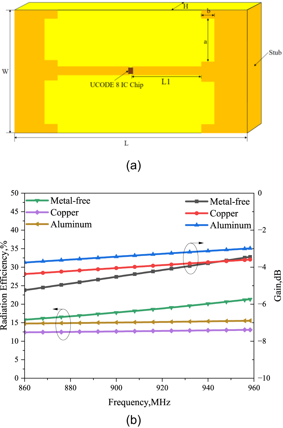
As shown in Figure 2(a), both ends of the feed line are connected to the backside by a shorting stub. A slot of length (a) and width (b) is etched near each stub to adjust impedance and accommodate the subsequent integration of asymmetric dipoles. To simulate performance on metal, 100 $\times$100 $\times$2 $\,\mathrm{mm}^{3}$ metal plates of different materials were placed beneath the antenna. Figure 2(b) shows the radiation efficiency and gain when placed on metal plates of different materials. It can be seen that this antenna structure has good metal-mountable interference characteristics.

Figure 2.

Radiation efficiency and gain on different metallic surfaces. (a) Structure configuration. (b) Radiation efficiency and gain.

Figure 2 Long description

The image A showing a rectangular structure drawing with dimension arrows and labels. The bottom edge is labeled L and the left edge is labeled W. A top dimension arrow is labeled H. Near the upper right, a vertical dimension is labeled a and a short horizontal dimension is labeled b. A right-side callout arrow points to the word Stub. A small square element on a central horizontal strip is labeled UCODE 8 IC Chip. A horizontal dimension along the central strip is labeled L1. The label (a) appears below the drawing. The image B showing a line graph with two vertical scales and a shared horizontal scale. The horizontal axis label reads Frequency,MHz, with tick labels 860, 880, 900, 920, 940, 960. The left vertical axis label reads Radiation Efficiency,% with tick labels from 0 to 50 in steps of 5. The right vertical axis label reads Gain,dB with tick labels 0, minus 2, minus 4, minus 6, minus 8, minus 10. Two legends appear at the top: on the left for radiation efficiency with entries Metal-free, Copper, Aluminum; on the right for gain with entries Metal-free, Copper, Aluminum. Radiation efficiency curves (left axis): Metal-free is a green line with downward triangle markers, increasing from about 16 at 860 to about 21 at 960. Copper is a purple line with diamond markers, near-flat from about 12.5 at 860 to about 13.5 at 960. Aluminum is a yellow line with left-pointing triangle markers, near-flat from about 14.5 at 860 to about 15.5 at 960. Gain curves (right axis): Metal-free is a gray line with square markers, increasing from about minus 5.2 at 860 to about minus 3.6 at 960. Copper is a red line with circle markers, increasing from about minus 4.4 at 860 to about minus 3.6 at 960. Aluminum is a blue line with upward triangle markers, increasing from about minus 3.8 at 860 to about minus 3.0 at 960. Two thin oval callouts are drawn on the plot: one around the radiation-efficiency region near frequency about 875 and one around the gain region near frequency about 935. The label (b) appears below the graph.

The current distribution on the antenna was simulated to illustrate its anti-metal operating mechanism. For clarity, the underlying copper plate is hidden in Figure 3. At the 0 $^{\circ}$ phase, the flow of the strongly resonant loop current along the vertical ring structure is clearly visible. This loop current exhibits a uniform, in-phase distribution, indicating a radiation pattern dominated by an effective magnetic dipole. The magnetic field generated by this current path is less affected by the metal in the near-field region. This mechanism avoids the performance degradation seen in electric dipoles, whose electric field is short-circuited by the metal. Consequently, this novel magnetic loop structure effectively improves radiation efficiency on metal surfaces.

Figure 3.

Surface current distribution of the magnetic loop structure. (a) Isometric view. (b) Top view.

Figure 3 Long description

Surface current distribution of the magnetic loop structure. (a) Isometric View. (b) Top View. The image A showing a simulation vector-field plot of surface current density labeled “Jsurf [A/m]”. The legend shows Min: 0.00e+00 and Max: 3.06e+01, with tick labels 3.06e+01, 2.72e+01, 2.38e+01, 2.04e+01, 1.70e+01, 1.36e+01, 1.02e+01, 6.80e+00, 3.40e+00, 0.00e+00. Arrow vectors are drawn across the conductor surface; arrows indicate surface-current direction and the color indicates the Jsurf magnitude in A/m. The highest values (near 3.06e+01 A/m) appear along a narrow central strip running lengthwise. Regions away from this strip transition through lower legend levels, reaching values near 0.00e+00 A/m at outer areas. A length scale is shown in millimeter with labels 0, 10, 20 mm. No labeled x-axis or y-axis is shown. The image B showing a simulation vector-field plot of the same quantity, “Jsurf [A/m]”, using the same legend range and tick labels (Min: 0.00e+00; Max: 3.06e+01). The geometry is shown in a top view with two larger rectangular areas separated by a narrow central connection region. Arrow vectors cover the surface; arrows indicate direction and the color indicates magnitude. The narrow central connection region contains the highest magnitudes, reaching near 3.06e+01 A/m, while areas farther from the connection show lower magnitudes that approach 0.00e+00 A/m near the outer boundary regions. A length scale is shown in millimeter with labels 0, 10, 20 mm. No labeled x-axis or y-axis is shown.

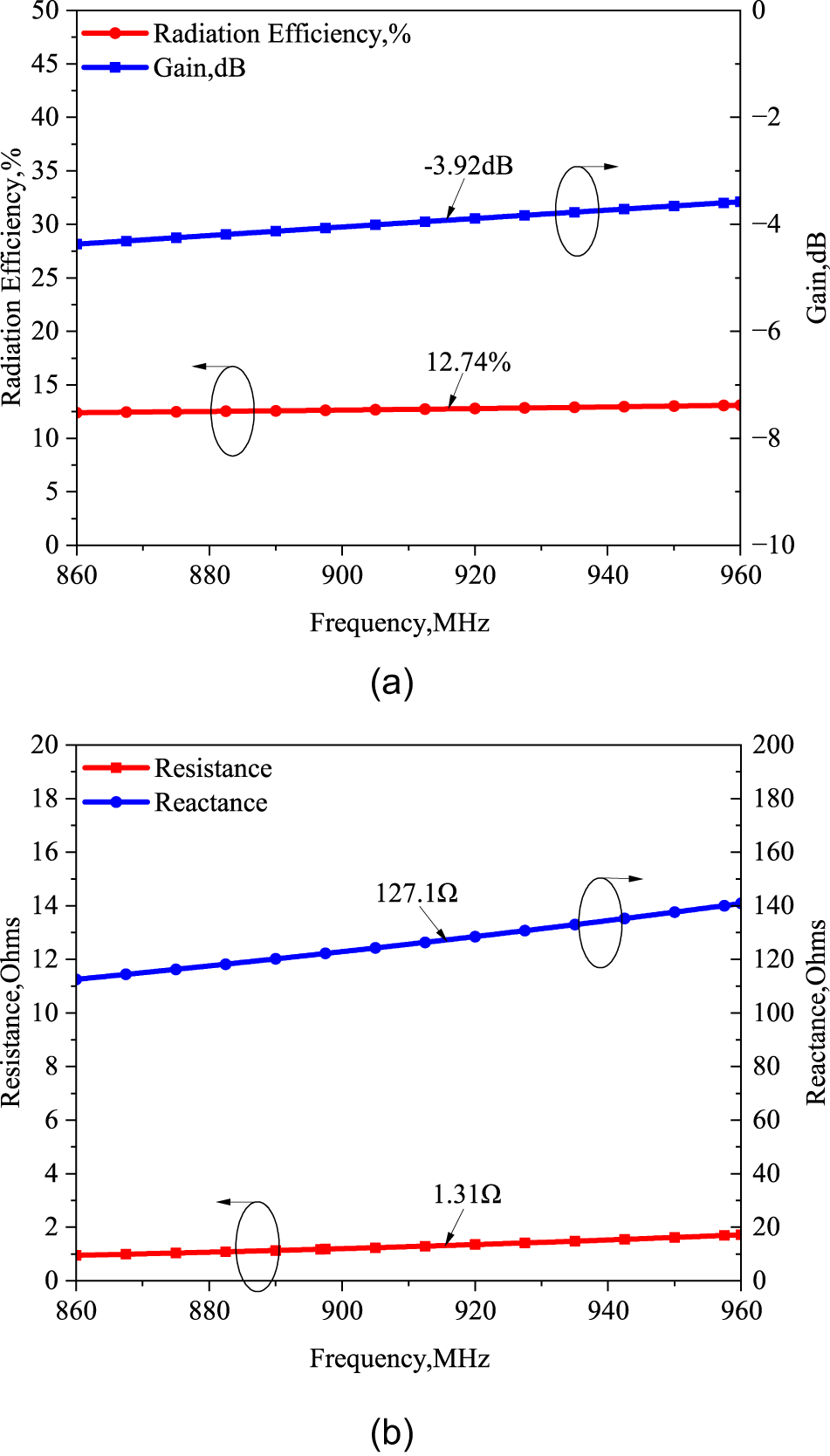
The corresponding input impedance, gain, and radiation efficiency on the copper plate are shown in Figure 4. The results show that a gain of $-$3.92 dBi and a radiation efficiency of 12.74% can be maintained despite the metal presence. However, the input impedance is severely mismatched with the tag chip.

Figure 4.

(a) Radiation efficiency and gain. (b) The resistance and reactance of antenna.

Figure 4 Long description

The image A showing a line graph with the legend “Radiation Efficiency,%” and “Gain,dB”. The horizontal axis label is “Frequency,MHz” with a range from 860 to 960. The left vertical axis label is “Radiation Efficiency,%” with a range from 0 to 50. The right vertical axis label is “Gain,dB” with a range from 0 to minus 10. The radiation efficiency line is nearly flat across the frequency range, with a text label “12.74 percent” pointing to the line. The gain line rises slightly across the frequency range, with a text label “-3.92dB” pointing to the line. The image B showing a line graph with the legend “Resistance” and “Reactance”. The horizontal axis label is “Frequency,MHz” with a range from 860 to 960. The left vertical axis label is “Resistance,Ohms” with a range from 0 to 20. The right vertical axis label is “Reactance,Ohms” with a range from 0 to 200. The resistance line rises slightly across the frequency range, with a text label “1.31Ω” pointing to the line. The reactance line rises across the frequency range, with a text label “127.1Ω” pointing to the line.

Although the vertical loop structure ensures stable radiation and metal-mount capability, the results in Figure 4 show severe impedance mismatch with the highly capacitive RFID chip. This is mainly attributed to the inherently single magnetic resonance of the loop, which indicates the necessity of introducing an additional controllable resonant mode.

The proposed antenna operates based on a hybrid magnetic–electric mode interaction mechanism, which fundamentally distinguishes it from conventional single-mode metal-mountable RFID tag antennas.

When the vertical loop structure is placed perpendicular to a metallic surface, the dominant radiation mechanism is governed by a magnetic dipole mode. The loop current forms a closed path normal to the metal plane, generating a magnetic field that satisfies the boundary condition 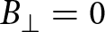${B_\perp=0}$ on a perfect conductor. As a result, the image current induced on the metal surface is in phase with the original loop current, which leads to constructive radiation rather than cancellation. This mechanism enables the vertical loop to maintain stable radiation performance in close proximity to metal.

However, a pure magnetic loop radiator typically exhibits a high quality factor (Q) and limited impedance tuning freedom. This characteristic restricts the achievable bandwidth and complicates conjugate matching with highly capacitive RFID chips.

To address this limitation, asymmetric bent dipole branches are introduced on both sides of the inductive feed line. These dipole branches primarily support an electric dipole mode, which is excited through near-field electromagnetic coupling rather than direct feeding.

The coexistence of magnetic and electric modes results in a dual-mode resonance behavior. The magnetic loop serves as the dominant radiator, ensuring metal-mount capability and radiation stability, while the electric dipole branches act as auxiliary resonators that introduce additional reactive paths. This interaction effectively reduces the overall radiation Q-factor and reshapes the input impedance trajectory, enabling broadband impedance matching without the need for lumped elements or multilayer structures.

More importantly, the two modes exhibit complementary frequency-shift tendencies in metallic environments. The resonance associated with the magnetic loop tends to shift upward due to reduced effective inductance near the metal surface, whereas the electric dipole resonance shifts downward owing to increased capacitive coupling. When properly designed, these opposite tendencies partially compensate for each other, resulting in enhanced resonance stability under metal loading.

Therefore, the proposed antenna does not rely on material engineering or artificial ground structures to achieve metal tolerance. Instead, it realizes broadband and stable on-metal performance through mode engineering at the structural level, by deliberately coupling magnetic and electric resonances within a compact single-layer configuration.

In RFID systems, the read range is a key performance metric. It defines the maximum distance at which a reader can reliably detect a tag’s backscattered signal. For passive UHF RFID systems, the maximum read range is mainly limited by the tag’s activation distance because the sensitivity of reader antenna is much higher. The maximum read range of a tag can be calculated using the Friis free-space transmission formula

(1)\begin{equation} {R_{tag}} = \frac{\lambda }{{4\pi }}\sqrt {\frac{{{P_t}{G_t}{G_r}\tau }}{{{P_{th}}}}}, \end{equation}

where ${P_t}$ is the transmit power of the reader antenna. ${G_t}$ is the gain of the reader antenna, and ${P_{th}}$ is the read sensitivity of the tag chip. ${G_r}$ is the gain of the tag antenna, and $\tau$ is the power transmission coefficient. $\tau$ can be calculated by

(2)\begin{equation} \tau = \frac{{4{R_A}{R_L}}}{{{{\left| {{Z_A} + {Z_L}} \right|}^2}}}, \end{equation}

where ${R_A}$ is the antenna resistance, and ${Z_A}$ is the antenna reactance. ${R_L}$ is the load resistance, and ${Z_L}$ is the load reactance [Reference Erman, Koziel, Lim, Leifsson, Hanafi and Murugesh8, Reference Murugesh, Lim, Chee and Bong14, Reference Sultan and Sabaawi18].

Therefore, impedance matching is a crucial step in designing UHF RFID tag antennas. It is difficult to achieve impedance matching by using only a magnetic loop structure, and its equivalent input impedance exhibits a typical series resonance response. ${{Z_{{\rm{in}}}}}$ is calculated by

(3)\begin{equation} {Z_{{\rm{in}}}} = R + j(\omega L - \frac{1}{{\omega C}}). \end{equation}

The dual-resonant design is inspired by gap-coupled patch technology, which enhances bandwidth performance by coupling two patches with different resonant frequencies to the same loop [Reference Nikitin, Brewster, Kim and Rao17]. Accordingly, asymmetric dipole structures are added on both sides of the feed line. Their flexible impedance characteristics enable precise conjugate matching with the tag chip. Its theoretical basis can be described by a dual-resonance equivalent circuit model and ${{Z_{{\rm{in}}}}}$ can be calculated by

(4)\begin{equation} {Z_{{\rm{in}}}} = {R_1} + j(\omega {L_1} - \frac{1}{{\omega {C_1}}}) + \frac{{j\omega {M^2}}}{{{R_2} + j(\omega {L_2} - \frac{1}{{\omega {C_2}}})}}, \end{equation}

where M is the mutual inductance coefficient between the loop feed line and the dipole arms.

To provide further physical insight into the proposed dual-resonant behavior, the antenna is interpreted using classical transmission-line and mutual coupling theory.

The vertical loop structure operates as a small-loop radiator whose circumference is electrically small compared with the operating wavelength. According to small-loop antenna theory, the loop mainly stores magnetic energy and can therefore be modeled as an inductive element. Its input impedance is obtained by

(5)\begin{equation} {Z_{\mathrm{loop}} = R_1 + j\omega L_1,} \end{equation}

where $R_1$ represents the radiation and ohmic losses, and $L_1$ denotes the equivalent inductance of the loop.

The meandered dipole branches located on both sides of the feeding strip behave as electrically lengthened dipole resonators. Each branch can be described using transmission-line theory as a terminated transmission-line section. The input impedance of the dipole branch is given by

(6)\begin{equation} {Z_{\mathrm{dipole}} = -j Z_0 \cot(\beta l_d),} \end{equation}

where $Z_0$ is the characteristic impedance, $\beta$ is the phase constant, and $l_d$ denotes the effective electrical length.

Since the dipole branches are not directly connected to the feeding port, energy transfer occurs through magnetic coupling between the loop current and the dipole currents. Based on mutual inductance theory, the induced voltage generated in the dipole branch produces a reflected impedance at the loop port, expressed as

(7)\begin{equation} {Z_{\mathrm{ref}} = \frac{(j\omega M)^2}{Z_{\mathrm{dipole}}},} \end{equation}

where $M$ denotes the mutual inductance between the loop and the dipole branches.

Accordingly, the overall equivalent impedance is obtained by

(8)\begin{equation} {Z_{\mathrm{in}} = Z_{\mathrm{loop}} + Z_{\mathrm{ref}} = R_1 + j\omega L_1 + \frac{(j\omega M)^2}{Z_{\mathrm{dipole}}}.} \end{equation}

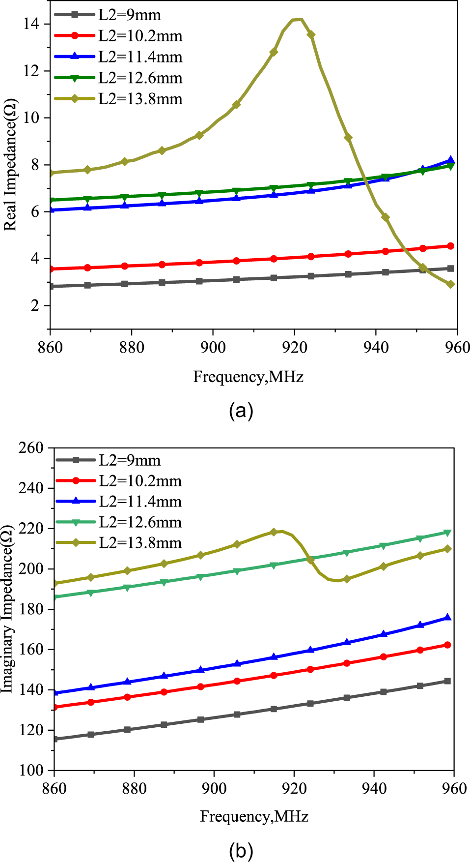
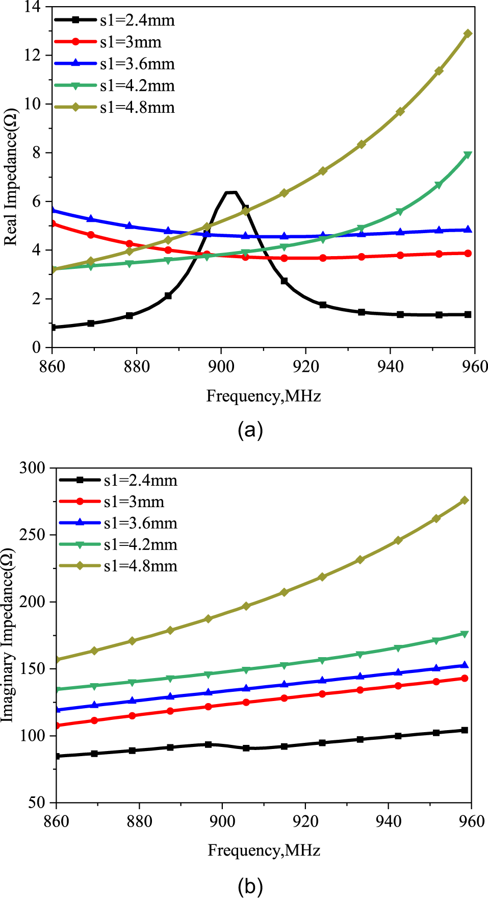
Figures 5 and 6 depict the effects of the dipole patch length (L2) and the spacing between the dipole patch and the feed line (s1) on the input impedance in a single-resonance antenna, with parameter L2 adjusted from 9 to 13.8 mm and parameter s1 adjusted from 2.4 to 4.8 mm. In these figures, it can be seen that the resonance frequency of the antenna decreases with the increase of L2 and s1, which indicates that L2 and s1 are effective parameters for coarse-tuning the resonance frequency.

Figure 5.

(a) The real impedance varying with L2. (b) The imaginary impedance varying with L2.

Figure 5 Long description

The image A showing a line graph labeled (a). The x-axis is labeled Frequency, megahertz, ranging from 860 to 960 with labeled ticks at 860, 880, 900, 920, 940 and 960. The y-axis is labeled Real Impedance, ohm, ranging from 2 to 14 with labeled ticks at 2, 4, 6, 8, 10, 12 and 14. A legend lists five series: L2 equals 9 millimeter, L2 equals 10.2 millimeter, L2 equals 11.4 millimeter, L2 equals 12.6 millimeter and L2 equals 13.8 millimeter. The L2 equals 9 millimeter series rises gradually from about 2.8 at 860 to about 3.6 at 960. The L2 equals 10.2 millimeter series rises gradually from about 3.5 at 860 to about 4.5 at 960. The L2 equals 11.4 millimeter series rises from about 6.1 at 860 to about 8.2 at 960. The L2 equals 12.6 millimeter series rises from about 6.5 at 860 to about 8.0 at 960. The L2 equals 13.8 millimeter series starts near about 7.7 at 860, increases to a peak near about 14.1 around 920, then decreases to about 9.2 around 935, about 5.8 around 945, about 3.6 around 952 and about 2.9 at 960. The image B showing a line graph labeled (b). The x-axis is labeled Frequency, megahertz, ranging from 860 to 960 with labeled ticks at 860, 880, 900, 920, 940 and 960. The y-axis is labeled Imaginary Impedance, ohm, ranging from 100 to 260 with labeled ticks at 100, 120, 140, 160, 180, 200, 220, 240 and 260. A legend lists five series: L2 equals 9 millimeter, L2 equals 10.2 millimeter, L2 equals 11.4 millimeter, L2 equals 12.6 millimeter and L2 equals 13.8 millimeter. The L2 equals 9 millimeter series increases from about 115 at 860 to about 145 at 960. The L2 equals 10.2 millimeter series increases from about 130 at 860 to about 162 at 960. The L2 equals 11.4 millimeter series increases from about 138 at 860 to about 176 at 960. The L2 equals 12.6 millimeter series increases from about 186 at 860 to about 218 at 960. The L2 equals 13.8 millimeter series increases from about 193 at 860 to about 219 around 918 to 920, then drops to about 195 around 930 and then increases to about 210 at 960.

Figure 6.

(a) The real impedance varying with s1. (b) The imaginary impedance varying with s1.

Figure 6 Long description

The image A showing a line graph with the vertical axis labeled Real Impedance(ohm) and the horizontal axis labeled Frequency,MHz. The horizontal axis range is 860 to 960. The vertical axis range is 0 to 14. The legend lists s1 equals 2.4 millimeter, s1 equals 3 millimeter, s1 equals 3.6 millimeter, s1 equals 4.2 millimeter and s1 equals 4.8 millimeter. s1 equals 2.4 millimeter: (860, 0.8), (870, 1.0), (880, 1.3), (890, 2.1), (900, 5.8), (905, 6.4), (910, 4.0), (915, 2.8), (920, 2.0), (930, 1.5), (940, 1.4), (950, 1.4), (960, 1.4) s1 equals 3 millimeter: (860, 5.0), (870, 4.6), (880, 4.2), (890, 4.0), (900, 3.8), (910, 3.7), (920, 3.7), (930, 3.7), (940, 3.8), (950, 3.8), (960, 3.9) s1 equals 3.6 millimeter: (860, 5.6), (870, 5.3), (880, 5.0), (890, 4.8), (900, 4.7), (910, 4.6), (920, 4.6), (930, 4.6), (940, 4.7), (950, 4.8), (960, 4.9) s1 equals 4.2 millimeter: (860, 3.2), (870, 3.3), (880, 3.4), (890, 3.6), (900, 3.7), (910, 3.9), (920, 4.2), (930, 4.6), (940, 5.1), (950, 6.0), (960, 7.9) s1 equals 4.8 millimeter: (860, 3.2), (870, 3.5), (880, 3.9), (890, 4.4), (900, 5.0), (910, 5.7), (920, 6.5), (930, 7.4), (940, 8.5), (950, 10.0), (960, 12.9) The image B showing a line graph with the vertical axis labeled Imaginary Impedance(ohm) and the horizontal axis labeled Frequency,MHz. The horizontal axis range is 860 to 960. The vertical axis range is 50 to 300. The legend lists s1 equals 2.4 millimeter, s1 equals 3 millimeter, s1 equals 3.6 millimeter, s1 equals 4.2 millimeter and s1 equals 4.8 millimeter. s1 equals 2.4 millimeter: (860, 85), (870, 87), (880, 89), (890, 91), (900, 93), (905, 90), (910, 91), (920, 94), (930, 97), (940, 99), (950, 101), (960, 104) s1 equals 3 millimeter: (860, 108), (870, 112), (880, 115), (890, 118), (900, 122), (910, 125), (920, 129), (930, 132), (940, 136), (950, 139), (960, 143) s1 equals 3.6 millimeter: (860, 120), (870, 123), (880, 126), (890, 129), (900, 132), (910, 136), (920, 140), (930, 143), (940, 146), (950, 149), (960, 152) s1 equals 4.2 millimeter: (860, 135), (870, 138), (880, 140), (890, 143), (900, 146), (910, 150), (920, 155), (930, 158), (940, 162), (950, 168), (960, 175) s1 equals 4.8 millimeter: (860, 155), (870, 162), (880, 170), (890, 178), (900, 187), (910, 197), (920, 210), (930, 222), (940, 235), (950, 255), (960, 275).

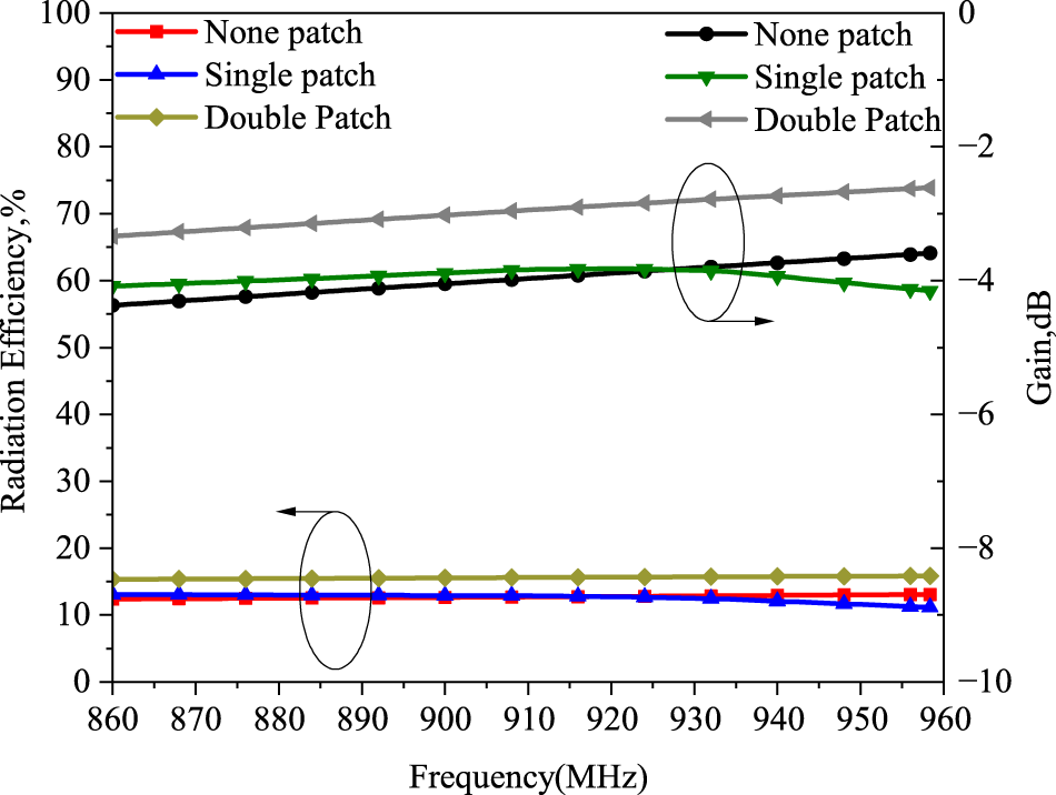
Embedding efficient dipole radiators into the loop structure will enhance the overall radiation efficiency and gain. Figure 7 compares the radiation efficiency and gain of the magnetic loop structure without a patch, a single coupled patch, and double patches. Figure 8 shows the maximum simulated realized gain for different configurations. Obviously, the dual-coupled antenna achieves higher radiation efficiency and gain than the single-coupled and basic loop designs under the same parameters. Therefore, the dual-coupled antenna was selected for our optimization.

Figure 7.

Radiation efficiency and gain for different antennas.

Figure 7 Long description

Radiation Efficiency and Gain for different antennas. A line graph with two vertical scales and one horizontal scale. The horizontal axis label is Frequency (megahertz), ranging from 860 to 960 with ticks every 10. The left vertical axis label is Radiation Efficiency, percent, ranging from 0 to 100 with ticks every 10. The right vertical axis label is Gain, decibel, ranging from 0 at the top to minus 10 at the bottom, with ticks at 0, minus 2, minus 4, minus 6, minus 8 and minus 10. Legend entries for radiation efficiency: None patch, Single patch, Double Patch. Legend entries for gain: None patch, Single patch, Double Patch. Radiation efficiency curves (left axis): None patch is a line with square markers. Values are about 12 to 13 percent from 860 to 960 megahertz, with a small rise toward the right end. Single patch is a line with triangle markers. Values are about 13 percent near 860 megahertz, staying near 13 percent through about 930 megahertz, then decreasing to about 11 to 12 percent by 960 megahertz. Double Patch is a line with diamond markers. Values are about 15 percent near 860 megahertz and increase slightly to about 16 percent by 960 megahertz. Gain curves (right axis): None patch is a line with circle markers. Values rise from about minus 4.4 decibel near 860 megahertz to about minus 3.6 decibel near 960 megahertz. Single patch is a line with downward triangle markers. Values are about minus 4.1 decibel near 860 megahertz, rise to about minus 3.8 decibel around 920 to 930 megahertz, then decrease to about minus 4.2 decibel by 960 megahertz. Double Patch is a line with left-pointing triangle markers. Values rise from about minus 3.3 decibel near 860 megahertz to about minus 2.6 decibel near 960 megahertz. Two thin ovals and arrows are drawn: one oval around the lower curves near about 885 to 890 megahertz with an arrow pointing left and one oval around the upper curves near about 930 to 935 megahertz with an arrow pointing right.

Figure 8.

Maximum simulated realized gain of the antenna. (a) None-patch. (b) Single-patch. (c) Double-patch antennas.

Figure 8 Long description

The figure consists of three 3D radiation-pattern surface plots labeled (a), (b) and (c), representing maximum simulated realized gain of antennas. Each plot shows dB(GainTotal) with a color scale indicating gain levels. The angular axes are labeled Phi in degrees and the radial magnitude represents gain in decibels. In image (a), the none-patch antenna has a maximum gain of -3.93 dB and a minimum of -37.41 dB. The plot shows a broad main lobe with no distinct sidelobes or nulls. In image (b), the single-patch antenna has a maximum gain of -3.72 dB and a minimum of -38.86 dB. The main lobe is slightly more focused compared to (a), with a small region of lower gain. In image (c), the double-patch antenna has a maximum gain of -2.33 dB and a minimum of -34.04 dB. The main lobe is more pronounced, with a higher peak gain and reduced null regions compared to (b). The color scale ranges from red (high gain) to blue (low gain), indicating the gain distribution across the surface. The plots illustrate how the antenna configuration affects gain patterns, with the double-patch showing the highest peak gain and the most focused main lobe.

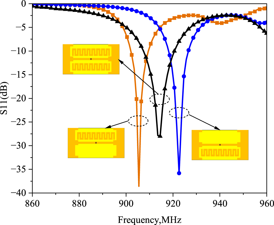
The coupling between the feed line and the patches allows us to adjust parameters L2 and s1 to tune the input impedance. We found two sets of parameters for the coupled patches, which create resonances below and above 915 MHz. Figure 9 shows the reflection coefficient (S11) of the proposed tag antenna under both single-resonant and dual-resonant conditions. Due to the complex nature of the chip impedance, S11 is calculated by

(9)\begin{equation} {S_{{\rm{11}}}} = \frac{{{Z_{{\rm{in}}}} - Z_{\rm{0}}^*}}{{{Z_{{\rm{in}}}} + {Z_{\rm{0}}}}}, \end{equation}

where ${{Z_{{\rm{in}}}}}$ is the antenna impedance and ${{Z_{\rm{0}}}}$ is the chip impedance. Figure 9 shows the return loss diagrams of single-resonance patches placed on the upper and lower layers of the feed line and dual-resonance patches. Dual-resonance occurs when both patches are coupled to the loop simultaneously. The results confirm that this modification effectively enhances the bandwidth and achieves optimized impedance matching.

Figure 9.

Reflection coefficient of the antenna in single-resonant and dual-resonant modes.

Figure 9 Long description

Reflection coefficient of the antenna in single-resonant and dual-resonant modes. A line graph with three plotted traces. The x-axis label is Frequency, megahertz, with tick labels 860, 880, 900, 920, 940, 960. The y-axis label is S11, decibel, with tick labels 0, minus 5, minus 10, minus 15, minus 20, minus 25, minus 30, minus 35, minus 40. One trace with square markers has a deep notch slightly above 900 megahertz, reaching about minus 39 decibel near about 905 megahertz. It rises to about minus 5 decibel by about 915 megahertz, stays around about minus 3 to minus 5 decibel through roughly 920 to 950 megahertz and approaches about 0 decibel near 960 megahertz. One trace with triangle markers has a notch centered between 910 and 920 megahertz, reaching about minus 28 decibel near about 915 megahertz. It is near about 0 to minus 5 decibel from about 860 to 900 megahertz, then drops toward the notch and returns to about minus 3 to minus 5 decibel from about 930 to 950 megahertz, ending near about minus 6 decibel at 960 megahertz. One trace with circular markers has a notch slightly above 920 megahertz, reaching about minus 36 decibel near about 922 megahertz. It is near about 0 decibel from about 860 to 900 megahertz, drops below minus 5 decibel around about 915 to 918 megahertz, reaches the minimum near about 922 megahertz, then rises to about minus 3 to minus 5 decibel by about 935 to 950 megahertz and is about minus 4 decibel near 960 megahertz. Three small inset schematic rectangles are shown inside the plot area, each connected by an arrow to a dashed oval near the corresponding notch region.

Although the operating bandwidth is broadened, the antenna still exhibits a relatively narrow impedance bandwidth in the lower frequency region, which is mainly determined by the magnetic loop resonance. In practical UHF RFID applications, region-specific frequency allocations do not require ultra-wide bandwidth. A stable resonance improves matching reliability and read consistency on metal surfaces.

From an application perspective, the proposed structure provides a balanced trade-off among compact size, mechanical simplicity, impedance controllability, and metal tolerance. The antenna maintains stable read range performance while avoiding complex multilayer or via-based structures. These characteristics make it suitable for industrial metal-tagging scenarios where robustness and cost efficiency are critical.

The current distribution of the dual-resonant antenna is shown in Figure 10. It can be seen that the surface currents are not confined to the feeding region but are effectively coupled to the two meandered dipole branches located on both sides of the vertical loop. The currents propagate continuously along the folded paths, which demonstrates that the meandered sections actively participate in resonance rather than acting as parasitic metallic parts.

Figure 10.

Surface current distribution of the dual-coupled patches. (a) Isometric view. (b) Top view.

Figure 10 Long description

Surface current distribution of the dual-coupled patches. (a) Isometric View. (b) Top View. The image A showing an isometric engineering field plot on a rectangular structure with arrows overlaid on a colored magnitude map. A legend is labeled “Jsurf (A m)” with tick labels 0e+000, 6e+000, 1.2e+001, 1.8e+001, 2.4e+001 and 3.0e+001. The structure includes a large rectangular ring trace, two inner rectangular regions filled with repeated narrow slot-like openings and a long narrow strip running through the middle. The highest legend range (near 3.0e+001) appears on the long narrow middle strip and at the small region where the strip meets the inner features. Lower legend ranges appear across the outer rectangular area. A scale bar is labeled 0, 15 and 30 mm. The label “(a)” appears under the scale bar. The image B showing a top view of the same structure with the same legend labeled “Jsurf (A m)” and the same tick labels 0e+000 through 3.0e+001. The long narrow middle strip and the small central region on that strip show the highest legend range (near 3.0e+001). The inner rectangular regions with repeated narrow slot-like openings show intermediate legend ranges and the outer area shows lower legend ranges. A scale bar is labeled 0, 15 and 30 mm. The label “(b)” appears under the scale bar.

The folded geometry increases the effective current path without enlarging the physical size, thereby extending the electrical length and enabling low-frequency resonance. Moreover, noticeable current intensity is maintained along the meandered arms, which indicates strong magnetic coupling between the vertical loop and the dipole branches. The induced currents generated through this coupling enhance the overall current magnitude and contribute to the formation of an additional resonant mode.

Therefore, the surface current distributions verify that the coupled meandered dipoles simultaneously realize electrical-length extension and current enhancement, which together lead to the proposed dual-resonant operation.

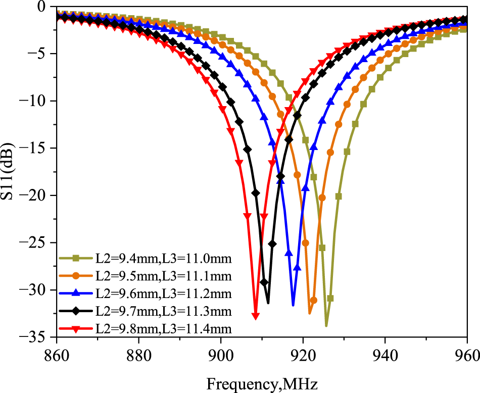
Furthermore, our antenna achieves active and controllable tuning of the center frequency through its structural parameters. By adjusting the dimensions of the asymmetric dipoles on both sides of the feed line, the shift in resonant frequency can be precisely controlled. Slots (length a, width b) are etched beside the resonant patches to meet different regional UHF band requirements. The center frequency of the tag antenna is effectively adjusted by varying the length of the asymmetric dipoles (L2, L3), as shown in Figure 11.

Figure 11.

The center frequencies varying with L2,L3.

Figure 11 Long description

S11(dB) A line graph with five plotted curves and a legend. The x-axis is labeled Frequency,MHz, ranging from 860 to 960 with labeled ticks at 860, 880, 900, 920, 940 and 960. The y-axis is labeled S11(dB), ranging from 0 at the top down to minus 35 at the bottom, with labeled ticks at 0, minus 5, minus 10, minus 15, minus 20, minus 25, minus 30 and minus 35. Legend entries: L2=9.4mm,L3=11.0mm L2=9.5mm,L3=11.1mm L2=9.6mm,L3=11.2mm L2=9.7mm,L3=11.3mm L2=9.8mm,L3=11.4mm All five curves start near 0 at 860 and return near 0 by 960, each forming one narrow minimum between about 910 and 930. L2=9.8mm,L3=11.4mm: minimum near 910 at about minus 33. L2=9.7mm,L3=11.3mm: minimum near 912 at about minus 31. L2=9.6mm,L3=11.2mm: minimum near 918 at about minus 31. L2=9.5mm,L3=11.1mm: minimum near 922 at about minus 32. L2=9.4mm,L3=11.0mm: minimum near 928 at about minus 34.

Impedance matching and radiation characteristics

Based on the design parameters provided in Table 1, the proposed tag antenna was simulated, fabricated, and measured sequentially. We adopted the dual-port S-parameter method to measure the input impedance, which is based on the principle of assuming the existence of a virtual metallic ground at the antenna’s symmetric center. Under this premise, the driving voltage can be decomposed into two components (V1 and V2), which are not affected by the distributed current of the antenna. The right arm of the dipole antenna and the virtual ground are regarded as Port 1, and the left arm and the virtual ground are regarded as Port 2. By measuring the S-matrix of this two-port network, all terms of the impedance Z-matrix can be obtained. ${{S_{11}}}$, ${{S_{12}}}$, ${{S_{21}}}$, and ${{S_{22}}}$ are measured, where ${{Z_0}}$ is the characteristic impedance of the semi-rigid coaxial cable used to fabricate the test fixture (50 $\Omega$) [Reference Nikitin, Brewster, Kim and Rao17, Reference Aslam, Kashif, Amin and Tenhunen21]. ${Z_d}$ can be calculated by

(10)\begin{equation} {Z_d} = \frac{{2{Z_0}(1 - {S_{11}}{S_{22}} + {S_{12}}{S_{21}} - {S_{12}} - {S_{21}})}}{{(1 - {S_{11}})(1 - {S_{22}}) - {S_{21}}{S_{22}}}} \end{equation}

As shown in Figure 12, the antenna was tested in free space and mounted on a 100 $\times$100 $\times$2 $\,\mathrm{mm}^{3}$ copper plate to simulate real-world metal deployment. A test fixture was made by soldering the outer conductors of two semi-rigid coaxial cables together. The fixture was connected to a Vector Network Analyzer. Port extension was applied to move the calibration reference plane to the ends of the fixture. Finally, the tag antenna under test was connected to the fixture. The antenna’s input impedance was calculated from the measured two-port S-parameters using Equation (4).

Figure 12.

Actual impedance measurement of the tag by vector network analyzer.

Figure 12 Long description

A vector network analyzer is displayed with a screen showing a waveform. Two semi-rigid coaxial cables are connected to the analyzer, extending to a test fixture on a copper plate. The setup is placed on a green surface, with a keyboard partially visible on the right side.

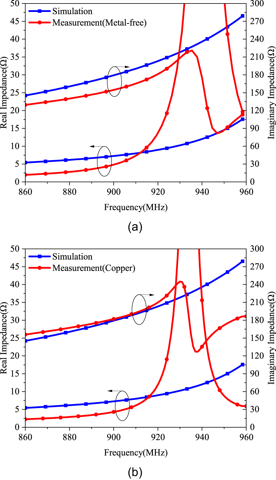
The measured data were substituted into Equation (4) to obtain the impedance diagram shown in Figure 13. It can be seen that even with certain errors, the antenna still maintains good impedance characteristics when closely attached to the metal plate.

Figure 13.

Measured and simulated impedance. (a) In free space. (b) On copper sheet.

Figure 13 Long description

The image A showing a dual y-axis line graph with a legend listing “Simulation” and “Measurement(Metal-free)”. The x-axis is labeled “Frequency(MHz)” and runs from 860 to 960 with labeled ticks at 860, 880, 900, 920, 940 and 960. The left y-axis is labeled “Real Impedance(Ω)” and runs from 0 to 50 with labeled ticks at 0, 5, 10, 15, 20, 25, 30, 35, 40, 45 and 50. The right y-axis is labeled “Imaginary Impedance(Ω)” and runs from 0 to 300 with labeled ticks at 0, 30, 60, 90, 120, 150, 180, 210, 240, 270 and 300. A blue square-marked curve for real impedance increases from about 24 at 860 to about 47 at 960. A red circle-marked curve for real impedance increases from about 22 at 860 to about 37 near the mid 930s, then is about 41 near the mid 950s and about 19 at 960. A blue square-marked curve for imaginary impedance increases from about 5 at 860 to about 18 at 960. A red circle-marked curve for imaginary impedance rises from about 2 at 860 to about 60 near 920, then forms a narrow peak reaching the top of the plotted range near the low 930s, then drops to about 90 near the mid 940s and is about 120 at 960. Two thin oval callouts and small arrows appear near the region around 900 on both the real-impedance and imaginary-impedance traces. The label “(a)” is centered below the plot. The image B showing a dual y-axis line graph with a legend listing “Simulation” and “Measurement(Copper)”. The x-axis is labeled “Frequency(MHz)” and runs from 860 to 960 with labeled ticks at 860, 880, 900, 920, 940 and 960. The left y-axis is labeled “Real Impedance(Ω)” and runs from 0 to 50 with labeled ticks at 0, 5, 10, 15, 20, 25, 30, 35, 40, 45 and 50. The right y-axis is labeled “Imaginary Impedance(Ω)” and runs from 0 to 300 with labeled ticks at 0, 30, 60, 90, 120, 150, 180, 210, 240, 270 and 300. A blue square-marked curve for real impedance increases from about 24 at 860 to about 47 at 960. A red circle-marked curve for real impedance increases from about 26 at 860 to about 40 near the low 930s, then is about 31 at 960. A blue square-marked curve for imaginary impedance increases from about 5 at 860 to about 18 at 960. A red circle-marked curve for imaginary impedance rises from about 2 at 860 to about 60 near 920, then forms a narrow peak reaching the top of the plotted range near the low 930s, then drops to about 120 near the high 930s and continues downward to about 30 at 960. Two thin oval callouts and small arrows appear near the region around 900 on both the real-impedance and imaginary-impedance traces. The label “(b)” is centered below the plot.

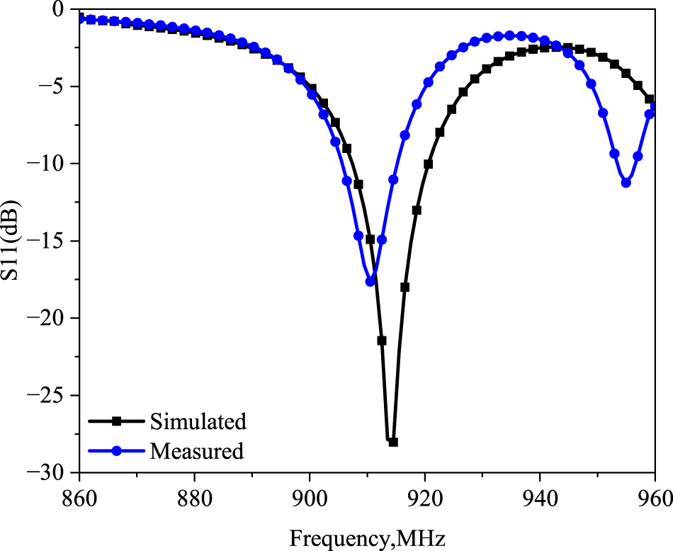
The measured impedance calculated from Figure 13(b) was substituted into Equation (9) to derive the measured S11; the simulated and measured S11 were shown in Figure 14.

Figure 14.

The simulation and measurement comparison of S11.

Figure 14 Long description

The y-axis label is S11 (dB). The y-axis ranges from 0 to minus 30, with labeled ticks at 0, minus 5, minus 10, minus 15, minus 20, minus 25 and minus 30. The x-axis label is Frequency, MHz. The x-axis ranges from 860 to 960, with labeled ticks at 860, 880, 900, 920, 940 and 960. A legend inside the plot lists two series: Simulated (black line with square markers) and Measured (blue line with circular markers). Simulated curve: Starts near 0 at 860, decreases gradually to around minus 3 to minus 4 by about 895 to 900, then drops to a minimum near 915 at about minus 28. It rises to around minus 4 by about 930, reaches around minus 3 near about 940 to 945, then declines to about minus 6 by 960. Measured curve: Starts near 0 at 860, decreases gradually to around minus 3 to minus 4 by about 895 to 900, then drops to a minimum near 910 to 912 at about minus 18. It rises to around minus 4 by about 925 to 930, reaches around minus 2 to minus 3 near about 935 to 940, then drops again to a second minimum near about 955 at about minus 11 and rises to about minus 6 by 960.

The simulated radiation pattern of the tag antenna at 915 MHz is shown in Figure 15. As shown by the radiation distribution in the $xy$-plane in Figure 15(a), the gain in the radiation pattern remains above $-$7 dB at 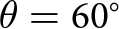$\theta = {60^{\circ}}$, and it can even exceed $-$4 dB at $\theta = {45^{\circ}}$. The radiation distributions in the $xz$-plane and $yz$-plane are shown in Figure 15(b). It shows that the main radiation coverage of this antenna is within these regions, which exhibits a sectorial radiation characteristic.

Figure 15.

(a) $XY$ plane read pattern. (b) $XZ$ and $YZ$ plane read pattern.

Figure 15 Long description

The first polar plot (a) shows the radiation pattern in the xy-plane with gain in decibels. The red trace indicates a nearly omnidirectional pattern with gain around minus 4 decibels, while the blue trace shows a more directional pattern with gain around minus 8 decibels. Key angles are marked at theta equals 45 degrees and theta equals 60 degrees. The second polar plot (b) displays the radiation pattern in the xz and yz planes. The red trace has a main lobe near phi equals 0 degrees with deep nulls reaching minus 12 to minus 14 decibels at lower angles. The blue trace maintains a more consistent gain between minus 4 and minus 6 decibels. These plots illustrate the antenna's sectorial radiation characteristics across different planes and angles.

Read range

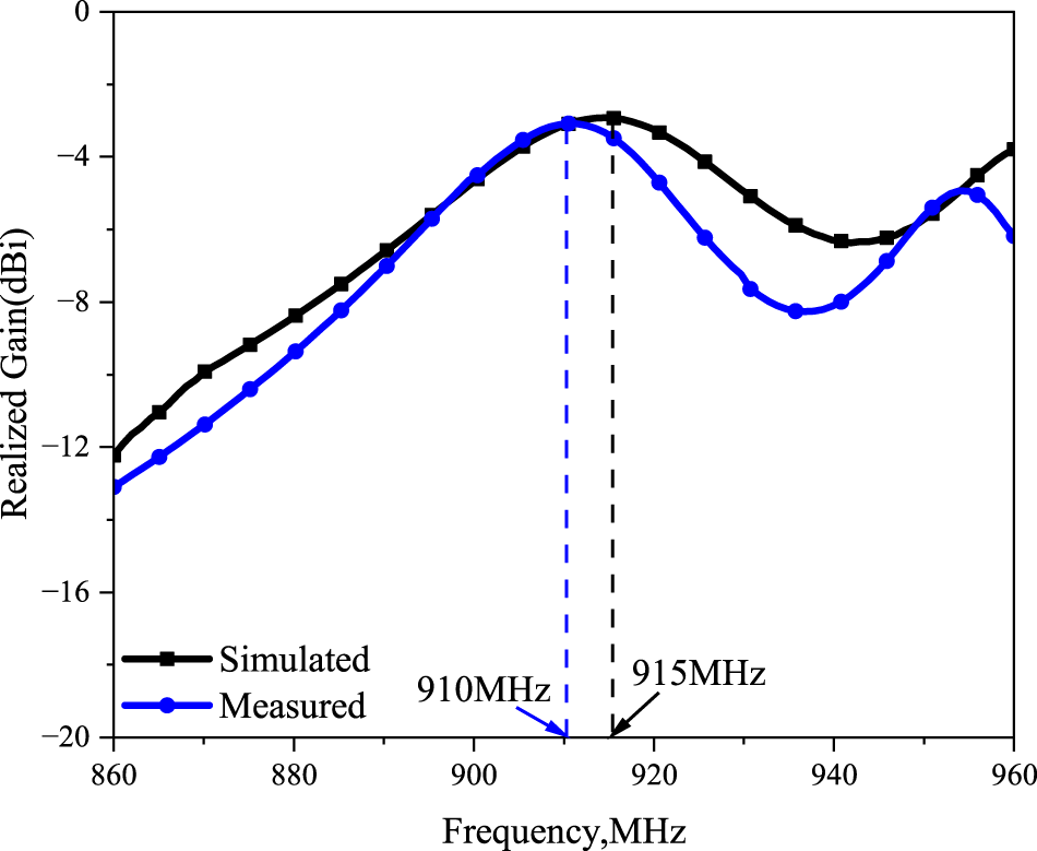
The tag was evaluated in an anechoic chamber, as shown in Figure 16. The realized gains of the proposed tag antenna for both simulation and measurement were compared in Figure 17. Referring to the same figure, the measured realized gain is $-$3.12 dBi at 0.910 GHz, which differs slightly from the simulated counterpart, $-$2.93 dBi at 0.915 GHz. The insignificant difference could be due to imperfection in the fabrication processes.

Figure 16.

Measurement of the recognition distance in darkroom.

Figure 16 Long description

The image shows a setup with a tag attached to a metal surface, labeled 'Tag on metal'. Below the tag, there is a label indicating the distance 'd'. In the foreground, a 'Reader Antenna' is positioned, with labels pointing to each component. The background features a textured surface, possibly for testing purposes.

Figure 17.

The measured and simulated gains of the antenna.

Figure 17 Long description

The line graph has a legend with two series: “Simulated” and “Measured”. The x-axis label is “Frequency,MHz”, with tick labels at 860, 880, 900, 920, 940 and 960. The y-axis label is “Realized Gain(dBi)”, with tick labels at 0, minus 4, minus 8, minus 12, minus 16 and minus 20. Two vertical dashed lines are marked with arrow labels “910MHz” and “915MHz”. Simulated series (square markers): At 860 the value is near minus 12. The curve rises to near minus 4 by about 900. It reaches a highest point near 915 at about minus 3 to minus 4. After that it decreases to around minus 6 to minus 7 near 940, then increases again toward about minus 4 by 960. Measured series (circle markers): At 860 the value is near minus 13. The curve rises to near minus 4 by about 900. It reaches a highest point near 910 at about minus 3 to minus 4. After that it decreases to around minus 8 near 940, then increases to around minus 5 near about 955 and ends near minus 6 at 960.

Then we measured the read range of the tag. The tag antenna was fixed first. Then we kept moving the reader antenna until the backscattered signal from the tag antenna was lost. The measured read range was 6.7 meters without a metal ground plane and 7.3 meters with it, which confirmed excellent metal-mount capability and practicality.

Comparison

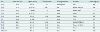
As summarized in Table 2, the performance of the proposed antenna was compared against several existing metal-mounted UHF RFID tag designs. The stub-loaded dipole proposed in [Reference Erman, Koziel, Lim, Leifsson, Hanafi and Murugesh8] was low-profile and achieved a read range of 9.75 m in the NA band by adopting a low-cost PTFE substrate. However, it could only switch between the NA and LEu dual bands and did not support wideband operation. In [Reference Murugesh, Rahim, Lim and Chee10], a patch-loaded loop antenna covered both LEu and NA bands by using a single-layer substrate, and it yielded an 8–9 m read range on metal containers. However, its performance was highly sensitive to layer alignment, with a 0.5 mm patch misalignment, which leads to impedance mismatch. The complementary coupled C-patch antenna presented in [Reference Murugesh, Lim, Chee and Bong14] attained wideband tuning from 920 MHz to 1.18 GHz and a read range of 9 m without relying on lumped components. However, it had drawbacks such as a large size, an inflexible foam substrate, and significant sensitivity to chip placement. The asymmetric SRR antenna in [Reference Ng, Lim, Chee and Murugesh15] supported independent LEu/NA tuning with a compact structure and achieved a read range of 5 m on a 20 $\times$20 cm metal plate. Yet, it required precise positioning of shorting pins to excite even/odd modes, as an offset of 0.5 mm caused a frequency detuning of over 5 MHz, and it exhibited low radiation efficiency, which was only 3–3.25%. [Reference Nguyen, Lin, Chang, Chen and Chen16] introduced a shorted C-patch antenna that was compact and low-cost. However, the narrow tuning range ( $\pm$5 MHz around 915 MHz) limited its regional adaptability. The low-profile PIFA in [Reference Inserra and Wen20] permitted post-fabrication tuning through a U-slot and lumped elements. Nevertheless, its read range was limited to 3.6 m, and the via-based shorting structure complicated the fabrication process, which reduced the production yield to below 85%. [Reference Aslam, Kashif, Amin and Tenhunen21] presented a magnetically coupled dual-resonance patch antenna that achieved an 11.5 m read range without shorting elements. However, it was large in size, sensitive to gaps, and restricted to the NA band. The stacked PILA in [Reference Ooi, Chee, Lim, Lee and Bong22] lowered the resonance frequency to 867 MHz via capacitive coupling, which resulted in a read range of 7.01–7.88 m. Yet, it required folding assembly and could only be tuned within a narrow band of 865–868 MHz. Finally, the zeroth-order serpentine antenna from [Reference Murugesh, Lim, Chee and Bong24] offered a planar omnidirectional radiation pattern, a read range of 8–9 m, and a low profile. However, it was bulky and its performance degraded by over 20% on uneven metal surfaces due to its double-layer stack structure.

Table 2.

Table of comparison between designed antenna and published work

Table 2 Long description

The table compares RFID tag antenna designs by reference, year, tag size, thickness, shorting elements, substrate, and achieved read range in meters. Read range spans from 3.6 m (Ref [20], 29.8×29.8 mm, 0.813 mm, vias, Rogers RO4003C) to 11.5 m (Ref [21], 118×42 mm, 1.6 mm, no shorting, Rogers 5880). Several 2024 designs without shorting elements report long ranges: 10.1 m on 6010LM-RT-Duroid at 39×39 mm and 9.5 m on PTFE with a 56 mm diameter tag. Foam-based designs vary from 7.2 m (31.5×31.5 mm with stubs) to 9.0 m (50×50 mm with no shorting) and 8.5 m (50×50 mm with walls). The presented “This Work” entry uses FR4, measures 64×42 mm, is 1.6 mm thick, uses stubs, and reports a 7.32 m read range, comparable to other mid-range results. Comparisons should be interpreted cautiously because size, substrate, and shorting approach differ across studies and can affect read range.

To further clarify the relative strengths of the proposed design, the main advantages and limitations are summarized as follows:

Advantages:

• • Stable on-metal performance ensured by the magnetic-dipole-dominated radiation mechanism.

• • Broadband impedance matching achieved through dual-resonant coupling.

• • Simple fabrication without multilayer stacking or via-based shorting walls.

• • Frequency controllability by tuning dipole lengths and coupling spacing.

Limitations:

• • The achievable gain is constrained by the compact aperture.

• • Performance may be affected by fabrication tolerance of the soldered shorting stubs.

In comparison, our tag design exhibits several distinct advantages. It adopts a simple single-substrate structure without folds or via interconnections, which enhances mechanical stability and reduces fabrication complexity. Unlike many existing designs that rely on material engineering or multilayer stacking, the proposed tag emphasizes structural-level mode and coupling engineering. This strategy enables wide frequency tuning without additional lumped elements, thereby improving cost-effectiveness. These results confirm its practicality for actual UHF RFID applications.