1 Introduction and formulation
In a Blasius boundary layer (and similar shear flows) it is well known that streamwise vorticity is highly efficient at generating streamwise streaks. At high Reynolds numbers, the asymptotically weak ‘roll’ motion associated with streamwise vorticity moves low-speed fluid from the wall into regions of higher streamwise velocity, with a return flow of higher-speed fluid towards the wall. This has been recognised for some time as a source of
 $O(1)$
low/high-speed streaks aligned with the free-stream direction. In the non-parallel context of the Blasius boundary layer, the in-plane roll motion and the downstream streak remain fully coupled, and herein we use the term ‘streak’ to indicate this three-dimensional disturbance on an otherwise two-dimensional Blasius boundary layer.
The role of streamwise streaks/vortices in transient growth has been extensively studied, see for example the discussion of Schmid & Henningson (Reference Schmid and Henningson2012). For boundary layers it is known (Andersson, Berggren & Henningson Reference Andersson, Berggren and Henningson1999) that the greatest amplification is associated with streaks that have spanwise scales comparable to the transverse boundary-layer thickness. The streak states that arise (Andersson et al. Reference Andersson, Brandt, Bottaro and Henningson2001) provide a primary structure on which secondary instabilities arise as the amplitude of the streak is increased. Of course the Blasius boundary layer is also unstable via the classical route of Tollmien–Schlichting (TS) waves, for sufficiently large Reynolds numbers. There is also evidence that artificially forcing streak states can stabilise a boundary layer to TS waves (Cossu & Brandt Reference Cossu and Brandt2002), so long as the streak amplitude remains below that required for a secondary instability.
Much of the analysis on ‘streaky’ boundary layers assumes periodicity in the spanwise direction. There are obviously some computational advantages to this assumption as well as empirical evidence of the importance of such states in flows disturbed by free-stream turbulence (for example). There are also a number of experimental investigations in which the disturbance is driven by spanwise-periodic distributions of wall roughness, injection or suction; see for example Bakchinov et al. (Reference Bakchinov, Grek, Klingmann and Kozlov1995) and White (Reference White2002). A notable exception is the experimental work of Asai, Minagawa & Nishioka (Reference Asai, Minagawa and Nishioka2002), in which a single streak perturbation is induced as a primary state, with the secondary instability induced via small harmonic oscillations imposed by injection through holes in the boundary surface.
Our focus in this work is spatially localised (rather than periodic) streaks, driven by wall forcing over a finite spanwise and streamwise extent; we begin with a theoretical linearised description before presenting analogous nonlinear streak states. Before developing our approach it is instructive to review some related theoretical results.
Linearised perturbations to a Blasius boundary layer have been considered in many contexts. Of particular relevance is the work of Libby & Fox (Reference Libby and Fox1963), which identified a set of two-dimensional (steady) eigenmodes that exist on a Blasius base state. The Libby & Fox modes are governed by the two-dimensional leading-order boundary-layer equation
 $$\begin{eqnarray}\unicode[STIX]{x1D6F7}_{Y}\unicode[STIX]{x1D6F7}_{Yx}-\unicode[STIX]{x1D6F7}_{x}\unicode[STIX]{x1D6F7}_{YY}=\unicode[STIX]{x1D6F7}_{YYY},\end{eqnarray}$$
where
 $\unicode[STIX]{x1D6F7}(x,Y)$
is a streamfunction,
 $x$
is a downstream coordinate and
 $Y$
is a rescaled boundary-layer coordinate. A solution exists in the form
 $$\begin{eqnarray}\unicode[STIX]{x1D6F7}(x,y)=(2x)^{1/2}\{F(\unicode[STIX]{x1D702})+\unicode[STIX]{x1D716}f(x,\unicode[STIX]{x1D702})\},\quad \text{with }\unicode[STIX]{x1D702}=Y/(2x)^{1/2},\end{eqnarray}$$
which then provides an evolution equation for perturbations
 $f$
of amplitude
 $\unicode[STIX]{x1D716}$
to the Blasius base state defined by
 $F$
, which satisfies
 $$\begin{eqnarray}F^{\prime \prime \prime }(\unicode[STIX]{x1D702})+F(\unicode[STIX]{x1D702})F^{\prime \prime }(\unicode[STIX]{x1D702})=0,\quad F(0)=F^{\prime }(0)=0,\quad F^{\prime }(\infty )=1.\end{eqnarray}$$
The perturbation
 $f(x,\unicode[STIX]{x1D702})$
represents a downstream evolving (linear, if
 $\unicode[STIX]{x1D716}\ll 1$
) perturbation. As shown by Libby & Fox (Reference Libby and Fox1963), a linearised solution for
 $f$
exists as a superposition of eigenmodes. These modal solutions take the form of
 $f(x,\unicode[STIX]{x1D702})=x^{-\unicode[STIX]{x1D70E}}\bar{f}(\unicode[STIX]{x1D702})$
, giving rise to a one-dimensional eigenvalue problem for the spatial (algebraic) decay ‘rate’
 $\unicode[STIX]{x1D70E}$
. The least-damped mode has
 $\unicode[STIX]{x1D70E}=1$
, for which an analytical solution was previously noted in the work of Stewartson (Reference Stewartson1957).
A closely related approach was later taken in the work of Luchini (Reference Luchini1996) albeit with a different emphasis. The focus of this later work is on three-dimensional modes, initially formulated for spanwise length scales that are comparable to the boundary-layer thickness, although a large spanwise wavelength limit is then taken. The goal was to gain insight into the transient growth mechanism associated with streak perturbations. The follow-up work of Luchini (Reference Luchini2000) went on to consider disturbances with a spanwise wavelength comparable to the boundary-layer thickness (including so-called optimal disturbances).
To place this three-dimensional formulation into a specific context, we consider a semi-infinite flat plate aligned with an oncoming incompressible, uniform flow of speed
 $U_{\infty }^{\ast }$
. An arbitrary choice of reference length scale,
 $L^{\ast }$
, allows for a non-dimensional Cartesian coordinate system
 $(L^{\ast }x,L^{\ast }y,L^{\ast }z)$
aligned with the leading edge of the plate at
 $x=0$
, such that
 $y=0,x>0$
defines the plate surface. To capture short spanwise scales typical of streaks we rescale in the
 $(y,z)$
plane according to
 $$\begin{eqnarray}(Y,Z)=Re^{1/2}(y,z).\end{eqnarray}$$
Here
 $Re=U_{\infty }^{\ast }L^{\ast }/\unicode[STIX]{x1D708}^{\ast }$
(for kinematic viscosity
 $\unicode[STIX]{x1D708}^{\ast }$
) is a global Reynolds number based on the chosen length scale. The corresponding high Reynolds number flow field (assumed to be steady) is
 $$\begin{eqnarray}u=\hat{U} (x,Y,Z)+\cdots \,,\quad (v,w)=Re^{-1/2}(\hat{V}(x,Y,Z),{\hat{W}}(x,Y,Z))+\cdots \,,\end{eqnarray}$$
with pressure
 $$\begin{eqnarray}p=Re^{-1/2}\hat{p}(x)+Re^{-1}\hat{P}(x,Y,Z)+\cdots \,.\end{eqnarray}$$
For large Reynolds number the solution is therefore governed by
 $$\begin{eqnarray}\displaystyle & \hat{U} \hat{U} _{x}+\hat{V}\hat{U} _{Y}+{\hat{W}}\hat{U} _{Z}=\hat{U} _{YY}+\hat{U} _{ZZ}, & \displaystyle\end{eqnarray}$$
 $$\begin{eqnarray}\displaystyle & \hat{U} \hat{V}_{x}+\hat{V}\hat{V}_{Y}+{\hat{W}}\hat{V}_{Z}=-\hat{P}_{Y}+\hat{V}_{YY}+\hat{V}_{ZZ}, & \displaystyle\end{eqnarray}$$
 $$\begin{eqnarray}\displaystyle & \hat{U} {\hat{W}}_{x}+\hat{V}{\hat{W}}_{Y}+{\hat{W}}{\hat{W}}_{Z}=-\hat{P}_{Z}+{\hat{W}}_{YY}+{\hat{W}}_{ZZ}, & \displaystyle\end{eqnarray}$$
 $$\begin{eqnarray}\displaystyle & \hat{U} _{x}+\hat{V}_{Y}+{\hat{W}}_{Z}=0. & \displaystyle\end{eqnarray}$$
 $Y=0$
) and matching to a uniform free stream in the far field. It has been previously employed in discussions of (spanwise-periodic) streaks (Higuera & Vega Reference Higuera and Vega2009), their transient growth (Luchini Reference Luchini1996, Reference Luchini2000; Andersson et al.
Reference Andersson, Berggren and Henningson1999) and their self-sustained interaction with travelling waves (Hall & Sherwin Reference Hall and Sherwin2010). Indeed, comparable governing equations have been employed in many other less directly related applications (including Rubin Reference Rubin1966; Hall Reference Hall1988; Dhanak & Duck Reference Dhanak and Duck1997; Goldstein et al.
Reference Goldstein, Sescu, Duck and Choudhari2016; Hewitt, Duck & Williams Reference Hewitt, Duck and Williams2017; Williams & Hewitt Reference Williams and Hewitt2017).
To tackle (1.6) Luchini (Reference Luchini1996) firstly assumed periodicity in
 $Z$
for a linear perturbation of the form
 $(u(x,Y),v(x,Y),w(x,Y))\exp (ikZ)$
added to a Blasius base flow. However, as noted in that work, taking this approach offers ‘no self-similarity, mainly because the two terms in the sum
 $u_{YY}-k^{2}u$
scale differently’. To avoid this issue, it was further assumed that
 $Re^{-1/2}\ll k\ll 1$
(implying small spanwise wavenumber), but three-dimensional effects were retained by allowing
 $kw\sim O(1)$
(the subsequent computational work of Luchini (Reference Luchini2000) corresponds to
 $k=O(1)$
). As for the Libby & Fox modes, solutions are again reduced to a one-dimensional eigenvalue problem by seeking separable states, for example
 $u(x,Y)=x^{-\unicode[STIX]{x1D707}}\bar{u}(\unicode[STIX]{x1D702})$
where
 $\unicode[STIX]{x1D702}$
is the transverse coordinate defined in (1.2). In this case it is found that
 $\unicode[STIX]{x1D707}\approx 0.787-1\approx -0.213$
, leading to algebraic growth of this (spanwise-periodic) perturbation. As we shall show, the value of
 $0.787\ldots$
turns out to be of relevance even to the localised three-dimensional streak eigenmodes discussed herein.
In this work we will not assume periodicity in the
 $Z$
coordinate, instead we seek solutions that solve (1.6) exactly, by retaining both the
 $Y$
and
 $Z$
dependence. In this sense these states are the natural three-dimensional extension of the Libby & Fox eigenmodes. Central to considering spatially localised streaks, we will require that the solution returns to the two-dimensional Blasius state as
 $|Z|\rightarrow \infty$
.
We first encompass the downstream growth of the transverse and spanwise length scales via a change of variables
 $$\begin{eqnarray}(\unicode[STIX]{x1D702},\unicode[STIX]{x1D701})=(2x)^{-1/2}(Y,Z).\end{eqnarray}$$
The transverse (
 $\unicode[STIX]{x1D702}$
) scale is well known from the Blasius solution (1.1)–(1.3), and for spanwise and transverse diffusion to remain comparable at all downstream positions we rescale
 $Z$
in the same manner. Similarly, for the velocity components
 $$\begin{eqnarray}\displaystyle & \hat{U} =U(x,\unicode[STIX]{x1D702},\unicode[STIX]{x1D701}), & \displaystyle\end{eqnarray}$$
 $$\begin{eqnarray}\displaystyle & (\hat{V},{\hat{W}})=(2x)^{-1/2}(\unicode[STIX]{x1D702}U(x,\unicode[STIX]{x1D702},\unicode[STIX]{x1D701})-\unicode[STIX]{x1D6F7}(x,\unicode[STIX]{x1D702},\unicode[STIX]{x1D701}),\unicode[STIX]{x1D701}U(x,\unicode[STIX]{x1D702},\unicode[STIX]{x1D701})-\unicode[STIX]{x1D6F9}(x,\unicode[STIX]{x1D702},\unicode[STIX]{x1D701})). & \displaystyle\end{eqnarray}$$
For a two-dimensional flow (that is,
 ${\hat{W}}\equiv 0$
) this formulation exactly mirrors the usual derivation of the Blasius similarity solution in terms a streamfunction
 $\unicode[STIX]{x1D6F7}$
, resulting in (1.3).
It is helpful to decompose the solution into a Blasius (two-dimensional) base flow governed by (1.3), plus a three-dimensional streak/roll contribution (denoted by tilde):
 $$\begin{eqnarray}U=F^{\prime }(\unicode[STIX]{x1D702})+\tilde{U} (x,\unicode[STIX]{x1D702},\unicode[STIX]{x1D701}),\quad \unicode[STIX]{x1D6F7}=F(\unicode[STIX]{x1D702})+\tilde{\unicode[STIX]{x1D6F7}}(x,\unicode[STIX]{x1D702},\unicode[STIX]{x1D701}),\end{eqnarray}$$
 $$\begin{eqnarray}\unicode[STIX]{x1D6F9}=\unicode[STIX]{x1D701}F^{\prime }(\unicode[STIX]{x1D702})+\tilde{\unicode[STIX]{x1D6F9}}(x,\unicode[STIX]{x1D702},\unicode[STIX]{x1D701}),\quad \unicode[STIX]{x1D6E9}=\unicode[STIX]{x1D701}F^{\prime \prime }(\unicode[STIX]{x1D702})+\tilde{\unicode[STIX]{x1D6E9}}(x,\unicode[STIX]{x1D702},\unicode[STIX]{x1D701}).\end{eqnarray}$$
The quantity
 $\unicode[STIX]{x1D6E9}$
is related to a vorticity component, and is introduced by a cross-differentiation to remove the pressure term from (1.6). It is worth emphasising that, as can be seen from (1.7),
 $\unicode[STIX]{x1D701}U-\unicode[STIX]{x1D6F9}$
is a measure of cross-flow and a three dimensional solution with
 ${\hat{W}}\neq 0$
is achieved for
 $\tilde{\unicode[STIX]{x1D6F9}}\neq \tilde{U}$
.
The fully nonlinear, three-dimensional parabolic system that represents the boundary-region equations (1.6) is now converted to:
 $$\begin{eqnarray}\hat{\unicode[STIX]{x1D6FB}}^{2}\tilde{\unicode[STIX]{x1D6F7}}=2\tilde{U} _{\unicode[STIX]{x1D702}}-\tilde{\unicode[STIX]{x1D6E9}}_{\unicode[STIX]{x1D701}}+2x\tilde{U} _{\unicode[STIX]{x1D702}x},\quad \hat{\unicode[STIX]{x1D6FB}}^{2}\tilde{\unicode[STIX]{x1D6F9}}=2\tilde{U} _{\unicode[STIX]{x1D701}}+\tilde{\unicode[STIX]{x1D6E9}}_{\unicode[STIX]{x1D702}}+2x\tilde{U} _{\unicode[STIX]{x1D701}x},\end{eqnarray}$$
 $$\begin{eqnarray}\hat{\unicode[STIX]{x1D6FB}}^{2}\tilde{U} =-F\tilde{U} _{\unicode[STIX]{x1D702}}-\tilde{\unicode[STIX]{x1D6F7}}F^{\prime \prime }-\tilde{\unicode[STIX]{x1D6F7}}\tilde{U} _{\unicode[STIX]{x1D702}}-\unicode[STIX]{x1D701}F^{\prime }\tilde{U} _{\unicode[STIX]{x1D701}}-\tilde{\unicode[STIX]{x1D6F9}}\tilde{U} _{\unicode[STIX]{x1D701}}+2xF^{\prime }\tilde{U} _{x}+2x\tilde{U} \tilde{U} _{x},\end{eqnarray}$$
 $$\begin{eqnarray}\displaystyle \hat{\unicode[STIX]{x1D6FB}}^{2}\tilde{\unicode[STIX]{x1D6E9}} & = & \displaystyle 2(\unicode[STIX]{x1D701}(F^{\prime }+\tilde{U} )\tilde{U} _{\unicode[STIX]{x1D702}}+\unicode[STIX]{x1D701}\tilde{U} F^{\prime \prime }-\unicode[STIX]{x1D702}(F^{\prime }+\tilde{U} )\tilde{U} _{\unicode[STIX]{x1D701}})\nonumber\\ \displaystyle & & \displaystyle -\,(F+\tilde{\unicode[STIX]{x1D6F7}})\tilde{\unicode[STIX]{x1D6E9}}_{\unicode[STIX]{x1D702}}-\unicode[STIX]{x1D701}\tilde{\unicode[STIX]{x1D6F7}}F^{\prime \prime \prime }-\tilde{\unicode[STIX]{x1D6F9}}(F^{\prime \prime }+\tilde{\unicode[STIX]{x1D6E9}}_{\unicode[STIX]{x1D701}})-\unicode[STIX]{x1D701}F^{\prime }\tilde{\unicode[STIX]{x1D6E9}}_{\unicode[STIX]{x1D701}}-2(F^{\prime }+\tilde{U} )\tilde{\unicode[STIX]{x1D6E9}}-2\tilde{U} \unicode[STIX]{x1D701}F^{\prime \prime },\nonumber\\ \displaystyle & & \displaystyle +\,2x((F^{\prime \prime }+\tilde{U} _{\unicode[STIX]{x1D702}})\tilde{\unicode[STIX]{x1D6F9}}_{x}-\tilde{U} _{\hat{\unicode[STIX]{x1D701}}}\tilde{\unicode[STIX]{x1D6F7}}_{x}+(F^{\prime }+\tilde{U} )\tilde{\unicode[STIX]{x1D6E9}}_{x}-(\unicode[STIX]{x1D701}F^{\prime \prime }+\tilde{\unicode[STIX]{x1D6E9}})\tilde{U} _{x}).\end{eqnarray}$$
This system is parabolic in
 $x$
, subject to the following no-slip and symmetry boundary conditions:
 $$\begin{eqnarray}\tilde{U} =\tilde{\unicode[STIX]{x1D6F9}}=\tilde{\unicode[STIX]{x1D6F7}}=0,\quad \tilde{\unicode[STIX]{x1D6E9}}=\tilde{\unicode[STIX]{x1D6F9}}_{\unicode[STIX]{x1D702}},\quad \text{on }\unicode[STIX]{x1D702}=0,\end{eqnarray}$$
 $$\begin{eqnarray}\tilde{U} _{\unicode[STIX]{x1D701}}=\tilde{\unicode[STIX]{x1D6F7}}_{\unicode[STIX]{x1D701}}=\tilde{\unicode[STIX]{x1D6E9}}=\tilde{\unicode[STIX]{x1D6F9}}=0,\quad \text{on }\unicode[STIX]{x1D701}=0.\end{eqnarray}$$
On approaching the free stream (
 $\unicode[STIX]{x1D702}\gg 1$
with
 $\unicode[STIX]{x1D701}$
fixed), following Hewitt & Duck (Reference Hewitt and Duck2014),
 $$\begin{eqnarray}\tilde{\unicode[STIX]{x1D6F7}}\sim \frac{A(x)\unicode[STIX]{x1D702}}{\unicode[STIX]{x1D701}^{2}+\unicode[STIX]{x1D702}^{2}},\quad \tilde{\unicode[STIX]{x1D6F9}}\sim \frac{A(x)\unicode[STIX]{x1D701}}{\unicode[STIX]{x1D701}^{2}+\unicode[STIX]{x1D702}^{2}},\end{eqnarray}$$
where
 $A$
is a constant determined as part of the solution, representing a measure of the far-field mass flux away/towards the streak into the free stream. For large
 $\unicode[STIX]{x1D701}$
near the boundary surface (
 $\unicode[STIX]{x1D702}=O(1)$
), there is a spanwise-decaying inner solution that must match (10d,e
) to the no-slip conditions at the surface. The details of this region are given in Hewitt & Duck (Reference Hewitt and Duck2014), but will be revisited in a related context in § 2.1. The arguments against algebraic decay towards the free stream made for traditional boundary-layer problems (see for example the discussions of, Brown & Stewartson Reference Brown and Stewartson1965; Hewitt, Duck & Stow Reference Hewitt, Duck and Stow2002) do not apply to the boundary-region equations as the vorticity decay remains exponential.
2 Spatially localised streak eigenmodes
The evolution of small-amplitude localised perturbations is governed by (1.9), under a linearisation assumption that neglects products of the disturbance
 $(\tilde{\unicode[STIX]{x1D6F7}},\tilde{\unicode[STIX]{x1D6F9}},\tilde{U} ,\tilde{\unicode[STIX]{x1D6E9}})$
. Given the form of (1.9) there are clearly downstream (decaying) disturbances proportional to
 $x^{\unicode[STIX]{x1D706}}$
. We may therefore seek linearised solutions of the form
 $$\begin{eqnarray}(\tilde{\unicode[STIX]{x1D6F7}},\tilde{\unicode[STIX]{x1D6F9}},\tilde{U} ,\tilde{\unicode[STIX]{x1D6E9}})=\unicode[STIX]{x1D716}x^{\unicode[STIX]{x1D706}}(\unicode[STIX]{x1D719}(\unicode[STIX]{x1D701},\unicode[STIX]{x1D702}),\unicode[STIX]{x1D713}(\unicode[STIX]{x1D701},\unicode[STIX]{x1D702}),u(\unicode[STIX]{x1D701},\unicode[STIX]{x1D702}),\unicode[STIX]{x1D703}(\unicode[STIX]{x1D701},\unicode[STIX]{x1D702}))+\cdots \,,\end{eqnarray}$$
which for
 $\unicode[STIX]{x1D716}\ll 1$
reduces (1.9) to a linear bi-global (generalised) eigenvalue problem for
 $\unicode[STIX]{x1D706}$
. We discretise the eigenproblem using a standard second-order central-difference discretisation of the
 $\unicode[STIX]{x1D701}{-}\unicode[STIX]{x1D702}$
plane, using a non-uniform grid, with a subsequent matrix eigenvalue analysis via the SLEPc library of Hernandez, Roman & Vidal (Reference Hernandez, Roman and Vidal2005). This is a substantial computation, with a sparse matrix eigenproblem of size
 $4N_{\unicode[STIX]{x1D702}}N_{\unicode[STIX]{x1D701}}\times 4N_{\unicode[STIX]{x1D702}}N_{\unicode[STIX]{x1D701}}$
, where
 $N_{\unicode[STIX]{x1D702},\unicode[STIX]{x1D701}}$
represents the number of nodal points in each direction.
If we were to ignore the
 $\unicode[STIX]{x1D701}$
dependence in (2.1) then we should expect to recover the (two-dimensional) eigenmodes of Libby & Fox (Reference Libby and Fox1963) outlined in (1.2). However, these do not satisfy our far-field requirement that modes are localised, i.e. they do not decay with
 $\unicode[STIX]{x1D701}$
. Nevertheless any eigenmode solutions to the linearised form of (1.9) may be viewed as new three-dimensional (localised) analogues of these classical states.
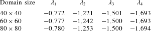
The first four eigenvalues (all real) obtained from the bi-global computation for domain truncations of the
 $(\unicode[STIX]{x1D701},\unicode[STIX]{x1D702})$
plane at
 $\unicode[STIX]{x1D701}=\unicode[STIX]{x1D702}=40,60,80$
.

In table 1 we provide numerical values (to three decimal places) for the first four localised eigenmodes. These values are obtained by fixing the domain size, then increasing the number of mesh points until the first four eigenvalues remain unchanged (to three decimal places) to any further refinement. Only after the eigenvalues are spatially resolved do we then recompute on a larger domain size to assess the influence of domain truncation. The resulting values for
 $\unicode[STIX]{x1D706}$
are robust to changes in both the number of nodal points in the computational mesh and the truncation of the computational domain. There are no other nearby eigenvalues in the region (
 $\unicode[STIX]{x1D706}_{r}>-1.7$
) spanned by these first four modes and the eigenvalues remain isolated/discrete. We have made no attempt to investigate the behaviour of the faster-decaying modes for
 $\unicode[STIX]{x1D706}_{r}<-1.7$
.
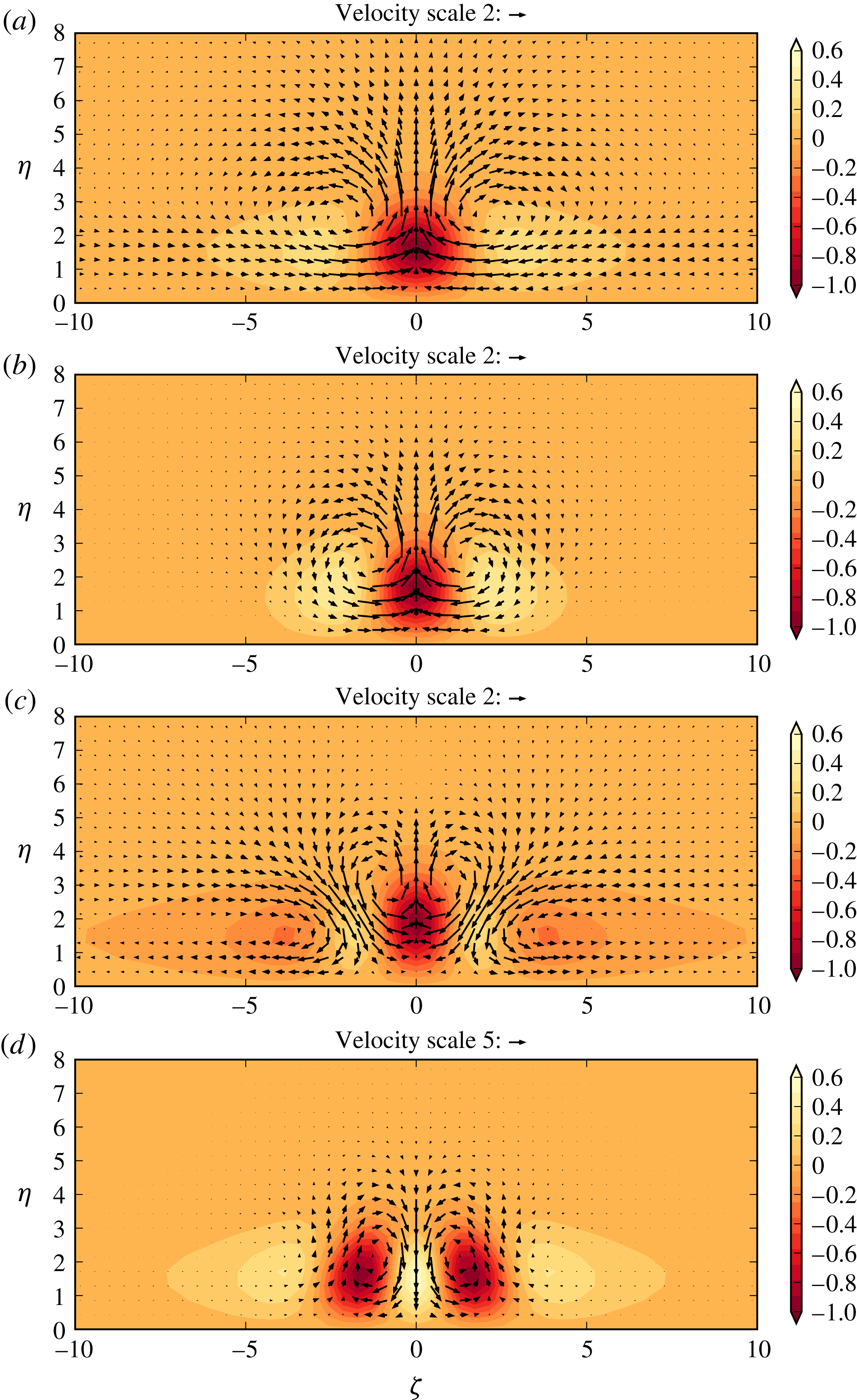
The first four localised eigenmodes for a Blasius flow (all real), normalised such that the largest perturbation to
 $u$
is
 $-1$
. Contours show the streamwise (streak) velocity component
 $u(\unicode[STIX]{x1D702},\unicode[STIX]{x1D701})$
, whilst the vector field shows the (in-plane) roll velocity components. These modes correspond to (a)
 $\unicode[STIX]{x1D706}_{1}$
, (b)
 $\unicode[STIX]{x1D706}_{2}$
, (c)
 $\unicode[STIX]{x1D706}_{3}$
and (d)
 $\unicode[STIX]{x1D706}_{4}$
, as given in table 1. A scale for length of the in-plane velocity vectors is noted at the top of each panel via a vector of magnitude 2 (a–c) and 5 (d).

The values of table 1 correspond to (real) eigenfunctions, which are shown in figure 1 over the
 $(\unicode[STIX]{x1D702},\unicode[STIX]{x1D701})$
plane. Each subfigure shows contours of the
 $u$
component of the eigenmode (normalised to make the minimum value
 $-1$
) and overlaid is the in-plane ‘roll’ velocity field
 $$\begin{eqnarray}(\unicode[STIX]{x1D702}u-\unicode[STIX]{x1D719},\unicode[STIX]{x1D701}u-\unicode[STIX]{x1D713}).\end{eqnarray}$$
Given these results, the perturbation velocity field at any required
 $x$
location can be obtained merely by rescaling of the
 $(\unicode[STIX]{x1D702},\unicode[STIX]{x1D701})$
coordinates and the in-plane velocities by
 $(2x)^{1/2}$
, as specified by (1.7).
It is immediately apparent from figure 1 that some modes decay more rapidly away from the streak, for example figure 1(b). This is particularly noticeable in the near-plate region (e.g.
 $\unicode[STIX]{x1D702}<2$
) where in some cases there is a marked cross-flow – that is, a non-zero
 ${\hat{W}}$
velocity component in the notation of (1.7). In all cases this cross-flow decays to zero for sufficiently large values of
 $\unicode[STIX]{x1D701}$
; note that figure 1 shows only a small section of the total computational domain.
2.1 A connection to the Libby & Fox (Reference Libby and Fox1963) and Luchini (Reference Luchini1996) eigenmodes
We have obtained three-dimensional (bi-global) eigenmodes that describe the downstream evolution of a single spatially isolated streak in a Blasius boundary layer. At first sight this may seem to be entirely disconnected from the two-dimensional eigenmodes of Libby & Fox (Reference Libby and Fox1963) and the (long-wavelength) spanwise-periodic states of Luchini (Reference Luchini1996) described in the introduction. However, we are able to relate a subset of the bi-global modes to both the work of Luchini and Libby & Fox by a careful consideration of the far-field behaviour. To achieve this, we will examine the flow far from the streak (
 $\unicode[STIX]{x1D701}\gg 1$
) and decompose the solution into an inner
 $\unicode[STIX]{x1D702}=O(1)$
layer matched to an outer
 $\unicode[STIX]{x1D702}=O(\unicode[STIX]{x1D701})$
region.
2.1.1 The inner
 $\unicode[STIX]{x1D702}=O(1)$
region for
$\unicode[STIX]{x1D701}\gg 1$


In the far field but still near to the boundary, that is
 $\unicode[STIX]{x1D701}\gg 1$
and
 $\unicode[STIX]{x1D702}=O(1)$
, we look for a spanwise decaying (
 $\unicode[STIX]{x1D6FD}>0$
) expansion for the eigenfunctions of (2.1) in the form
 $$\begin{eqnarray}(\unicode[STIX]{x1D719},\unicode[STIX]{x1D713},u,\unicode[STIX]{x1D703})=(\bar{\unicode[STIX]{x1D719}}(\unicode[STIX]{x1D702})\unicode[STIX]{x1D701}^{-(\unicode[STIX]{x1D6FD}+1)},\bar{\unicode[STIX]{x1D713}}(\unicode[STIX]{x1D702})\unicode[STIX]{x1D701}^{-\unicode[STIX]{x1D6FD}},\bar{u}(\unicode[STIX]{x1D702})\unicode[STIX]{x1D701}^{-(\unicode[STIX]{x1D6FD}+1)},\bar{\unicode[STIX]{x1D703}}(\unicode[STIX]{x1D702})\unicode[STIX]{x1D701}^{-\unicode[STIX]{x1D6FD}})+\cdots \,.\end{eqnarray}$$
For an expansion in the form of (2.3), the governing equations (1.9) provide a leading-order ordinary-differential system for
 $\unicode[STIX]{x1D701}\gg 1$
of
 $$\begin{eqnarray}\displaystyle & \bar{\unicode[STIX]{x1D719}}_{\unicode[STIX]{x1D702}}=(2+2\unicode[STIX]{x1D706})\bar{u}+\unicode[STIX]{x1D6FD}\bar{\unicode[STIX]{x1D713}}, & \displaystyle\end{eqnarray}$$
 $$\begin{eqnarray}\displaystyle & \bar{u}_{\unicode[STIX]{x1D702}\unicode[STIX]{x1D702}}=(2\unicode[STIX]{x1D706}+\unicode[STIX]{x1D6FD}+1)\bar{u}F^{\prime }-F\bar{u}_{\unicode[STIX]{x1D702}}-F^{\prime \prime }\bar{\unicode[STIX]{x1D719}}, & \displaystyle\end{eqnarray}$$
 $$\begin{eqnarray}\displaystyle & \bar{\unicode[STIX]{x1D713}}_{\unicode[STIX]{x1D702}\unicode[STIX]{x1D702}}=(2\unicode[STIX]{x1D706}+\unicode[STIX]{x1D6FD}-1)(\bar{\unicode[STIX]{x1D713}}-\bar{\unicode[STIX]{x1D713}}(\infty ))F^{\prime }-F\bar{\unicode[STIX]{x1D713}}_{\unicode[STIX]{x1D702}}-F^{\prime \prime }\bar{\unicode[STIX]{x1D719}}+2F^{\prime }\bar{u}, & \displaystyle\end{eqnarray}$$
 $\unicode[STIX]{x1D703}$
equation arising from (1.9). At the boundary, no-slip and impermeability conditions give
 $\bar{u}=\bar{\unicode[STIX]{x1D719}}=\bar{\unicode[STIX]{x1D713}}=0$
whilst
 $\bar{u}\rightarrow 0$
and
 $\bar{\unicode[STIX]{x1D713}}\rightarrow \bar{\unicode[STIX]{x1D713}}(\infty )$
as
 $\unicode[STIX]{x1D702}\rightarrow \infty$
. The quantity
 $\bar{\unicode[STIX]{x1D713}}(\infty )$
is in general unknown and must ultimately be determined by an outer solution for
 $\unicode[STIX]{x1D702},\unicode[STIX]{x1D701}\gg 1$
, which we will discuss below.
In physical terms, as can be seen from the similarity form of (1.7c
) and the decomposition (2.3), the cross-flow velocity associated with this perturbation is proportional to
 $\bar{u}-\bar{\unicode[STIX]{x1D713}}$
. Because
 $\bar{u}\rightarrow 0$
for
 $\unicode[STIX]{x1D702}\gg 1$
, we see that
 $\bar{\unicode[STIX]{x1D713}}(\infty )$
is essentially a measure of cross-flow at the base of the outer region.
Somewhat surprisingly, we can still relate (2.4) to the (non-localised) eigenmodes discussed by Libby & Fox (Reference Libby and Fox1963) and Luchini (Reference Luchini1996). To do this we introduce
 $h=\bar{u}-\bar{\unicode[STIX]{x1D713}}$
, which is related to the amount of cross-flow, and eliminate
 $\bar{u}$
. This reformulation leads to
 $$\begin{eqnarray}\displaystyle & \bar{\unicode[STIX]{x1D719}}_{\unicode[STIX]{x1D702}\unicode[STIX]{x1D702}\unicode[STIX]{x1D702}}+F\bar{\unicode[STIX]{x1D719}}_{\unicode[STIX]{x1D702}\unicode[STIX]{x1D702}}+F^{\prime \prime }\bar{\unicode[STIX]{x1D719}}+(2\unicode[STIX]{x1D706}+\unicode[STIX]{x1D6FD}+1)(F^{\prime \prime }\bar{\unicode[STIX]{x1D719}}-F^{\prime }\bar{\unicode[STIX]{x1D719}}_{\unicode[STIX]{x1D702}})=\unicode[STIX]{x1D6FD}(2F^{\prime }h+(2\unicode[STIX]{x1D706}+\unicode[STIX]{x1D6FD}-1)h(\infty )), & \displaystyle \nonumber\\ \displaystyle & & \displaystyle\end{eqnarray}$$
 $$\begin{eqnarray}\displaystyle & h_{\unicode[STIX]{x1D702}\unicode[STIX]{x1D702}}=(2\unicode[STIX]{x1D706}+\unicode[STIX]{x1D6FD}-1)(F^{\prime }h-h(\infty ))-Fh_{\unicode[STIX]{x1D702}}, & \displaystyle\end{eqnarray}$$
 $h(\infty )=-\bar{\unicode[STIX]{x1D713}}(\infty )$
. For
 $h(\infty )\neq 0$
there is always a forced solution available to (2.5), which is an issue we will revisit below.
In both the homogeneous (
 $h(\infty )=0$
) and inhomogeneous (
 $h(\infty )\neq 0$
) cases, the corresponding solutions for
 $\bar{\unicode[STIX]{x1D719}}$
(and hence
 $\bar{u}$
,
 $\bar{\unicode[STIX]{x1D703}}$
) are obtained from (2.5a
), which is forced by
 $h$
. In particular we note that
 $$\begin{eqnarray}\bar{\unicode[STIX]{x1D719}}\sim -\unicode[STIX]{x1D6FD}h(\infty )\unicode[STIX]{x1D702}+d,\end{eqnarray}$$
for a constant
 $d$
when
 $\unicode[STIX]{x1D702}$
is large.
In the absence of any leading-order cross-flow at the base of the outer layer (
 $h(\infty )=0$
) a possible solution is obviously
 $h\equiv 0$
, in which case (2.5a
) reduces to the problem first considered by Libby & Fox (Reference Libby and Fox1963). With some minor rescaling, we obtain precisely the Libby & Fox eigenproblem, or equivalently equation (4) from the discussion of Luchini (Reference Luchini1996). These eigenmodes therefore exist with the following discrete values
 $$\begin{eqnarray}\unicode[STIX]{x1D706}+\frac{\unicode[STIX]{x1D6FD}+1}{2}\approx -1,-1.887,-2.814,\ldots .\end{eqnarray}$$
Furthermore, if
 $h(\unicode[STIX]{x1D702})\not \equiv 0$
, but with
 $h(\infty )=0$
, again, some minor rescaling of
 $\unicode[STIX]{x1D702}$
reduces the decoupled problem for
 $h$
to (Luchini Reference Luchini1996, equation (9)), with the eigenvalue
 $s$
in that work replaced by
 $\unicode[STIX]{x1D706}+(\unicode[STIX]{x1D6FD}-1)/2$
. In this scenario therefore, there exist discrete eigenmode solutions to (2.5) with
 $$\begin{eqnarray}\unicode[STIX]{x1D706}+\frac{\unicode[STIX]{x1D6FD}-1}{2}\approx -0.787,-1.694,-2.627,\ldots .\end{eqnarray}$$
Note that the numerical values on the right-hand sides of (2.7) and (2.8) are provided in (Luchini Reference Luchini1996, tables 1 and 2).
The inner
 $\unicode[STIX]{x1D702}=O(1)$
behaviour therefore has three possibilities, (i)
 $h(\infty )\neq 0$
leading to a forced solution driven by cross-flow at the base of an outer region, (ii)
 $h(\infty )=0$
with a Libby & Fox eigenmode that is free of cross-flow at leading order or (iii)
 $h(\infty )=0$
with a Luchini eigenmode that has a jet-like cross-flow that decays on approaching the outer region.
2.1.2 The outer
$\unicode[STIX]{x1D702}=O(\unicode[STIX]{x1D701})$
region for
$\unicode[STIX]{x1D701}\gg 1$


At this stage of the discussion, the spanwise decay of the localised mode is determined by
 $\unicode[STIX]{x1D6FD}$
, which is a free parameter, and any pair of (
 $\unicode[STIX]{x1D706},\unicode[STIX]{x1D6FD}$
) satisfying (2.7) or (2.8) is valid. However, we have yet to impose matching conditions as
 $\unicode[STIX]{x1D702}\rightarrow \infty$
, for which we need to determine the outer flow.
In the outer region
 $\unicode[STIX]{x1D701},\unicode[STIX]{x1D702}\gg 1$
,
 $u$
and
 $\unicode[STIX]{x1D703}$
are negligible whilst
 $\unicode[STIX]{x1D719}$
and
 $\unicode[STIX]{x1D713}$
are harmonic. In polar coordinates
 $r=(\unicode[STIX]{x1D701}^{2}+\unicode[STIX]{x1D702}^{2})^{1/2}\gg 1$
and
 $\unicode[STIX]{x1D6FC}=\arctan (\unicode[STIX]{x1D702}/\unicode[STIX]{x1D701})$
, this leads to
 $$\begin{eqnarray}\displaystyle & \unicode[STIX]{x1D719}=a_{1}r^{-1}\sin (\unicode[STIX]{x1D6FC})+a_{2}r^{-2}\cos (2\unicode[STIX]{x1D6FC})+a_{3}r^{-3}\sin (3\unicode[STIX]{x1D6FC})+\ldots , & \displaystyle\end{eqnarray}$$
 $$\begin{eqnarray}\displaystyle & \unicode[STIX]{x1D713}=a_{1}r^{-1}\cos (\unicode[STIX]{x1D6FC})-a_{2}r^{-2}\sin (2\unicode[STIX]{x1D6FC})+a_{3}r^{-3}\cos (3\unicode[STIX]{x1D6FC})+\ldots , & \displaystyle\end{eqnarray}$$
 $\unicode[STIX]{x1D719}$
(and antisymmetry of
 $\unicode[STIX]{x1D713}$
) about
 $\unicode[STIX]{x1D701}=0$
(that is,
 $\unicode[STIX]{x1D6FC}=\unicode[STIX]{x03C0}/2$
). In effect, this is a generalisation of the far-field boundary conditions discussed by Hewitt & Duck (Reference Hewitt and Duck2014). On approaching the
 $\unicode[STIX]{x1D702}=0$
boundary (
 $\unicode[STIX]{x1D6FC}\rightarrow 0$
) from the outer region, we obtain
 $$\begin{eqnarray}\displaystyle & \displaystyle \unicode[STIX]{x1D719}=\frac{a_{1}\unicode[STIX]{x1D702}+a_{2}}{\unicode[STIX]{x1D701}^{2}}+\frac{-a_{1}\unicode[STIX]{x1D702}^{3}-3a_{2}\unicode[STIX]{x1D702}^{2}+3a_{3}\unicode[STIX]{x1D702}+a_{4}}{\unicode[STIX]{x1D701}^{4}}+\cdots \,, & \displaystyle\end{eqnarray}$$
 $$\begin{eqnarray}\displaystyle & \displaystyle \unicode[STIX]{x1D713}=\frac{a_{1}}{\unicode[STIX]{x1D701}}+\frac{-a_{1}\unicode[STIX]{x1D702}^{2}-2a_{2}\unicode[STIX]{x1D702}+a_{3}}{\unicode[STIX]{x1D701}^{3}}+\cdots \,. & \displaystyle\end{eqnarray}$$
 $\unicode[STIX]{x1D702}=O(1)$
inner region and the
 $\unicode[STIX]{x1D702}=O(\unicode[STIX]{x1D701})$
outer solution we must clearly match solutions of (2.5) for large
 $\unicode[STIX]{x1D702}$
with (2.10). The values
 $a_{i}$
are determined globally as part of the bi-global eigenvalue problem (to within a normalisation).
2.2 Classification of the first four computed eigenmodes
Having identified the types of behaviour that can occur, we may now classify the first four eigenvalues (
 $\unicode[STIX]{x1D706}_{1},\ldots ,\unicode[STIX]{x1D706}_{4}$
) presented in table 1, according to their large-
 $\unicode[STIX]{x1D701}$
behaviour as described in § 2.1. In particular, we find that the first and fourth modes,
 $\unicode[STIX]{x1D706}=\unicode[STIX]{x1D706}_{1,4}$
have far-field behaviour comparable to the Luchini (Reference Luchini1996) modes, with
 $h(\infty )=0$
in the notation of § 2.1. The other two modes of table 1 are associated with the case
 $h(\infty )\neq 0$
and remain distinct.
2.2.1 Modes linked to those of Libby & Fox (Reference Libby and Fox1963) and Luchini (Reference Luchini1996):
$h(\infty )=0$

If
 $a_{1}=0$
but
 $a_{2}\neq 0$
then (2.10) shows that
 $\unicode[STIX]{x1D713}=o(1/\unicode[STIX]{x1D701})$
as
 $\unicode[STIX]{x1D702}\rightarrow 0$
for large
 $\unicode[STIX]{x1D701}$
. However
 $\unicode[STIX]{x1D719}=O(1/\unicode[STIX]{x1D701}^{2})$
, which therefore requires that
 $\unicode[STIX]{x1D6FD}=1$
in (2.3). This lack of a (leading-order, near-boundary) cross-flow in the outer solution as
 $\unicode[STIX]{x1D6FC}\rightarrow 0$
means that
 $h(\infty )=0$
. In this case, equation (2.5) is reduced to a one-dimensional eigenvalue problem for
 $\unicode[STIX]{x1D706}$
. One option is that, near the plate the eigensolution connected to the Luchini eigenmodes develop, as determined by (2.8), leading to (as
 $\unicode[STIX]{x1D6FD}=1$
)
 $$\begin{eqnarray}\unicode[STIX]{x1D706}\approx -0.787,-1.694,\ldots .\end{eqnarray}$$
A second possibility is that the response takes the form of a Libby & Fox eigenmode determined by (2.7), such that (on taking
 $\unicode[STIX]{x1D6FD}=1$
):
 $$\begin{eqnarray}\unicode[STIX]{x1D706}\approx -2,-2.887,\ldots .\end{eqnarray}$$
Clearly the Libby & Fox modes are faster decaying (in
 $x$
), and therefore do not dominate the far-downstream response of the flow. The least-damped modes are connected to those of Luchini, and as such are obtained in the (
 $\unicode[STIX]{x1D701}\gg 1$
) far field of the bi-global eigenmodes shown in figure 1(a,d) where
 $\unicode[STIX]{x1D706}=\unicode[STIX]{x1D706}_{1}\approx -0.787$
and
 $\unicode[STIX]{x1D706}=\unicode[STIX]{x1D706}_{4}\approx -1.694$
respectively.
To validate this asymptotic description we compare the predicted large-
 $\unicode[STIX]{x1D701}$
behaviour for the first eigenmode (
 $\unicode[STIX]{x1D706}=\unicode[STIX]{x1D706}_{1}$
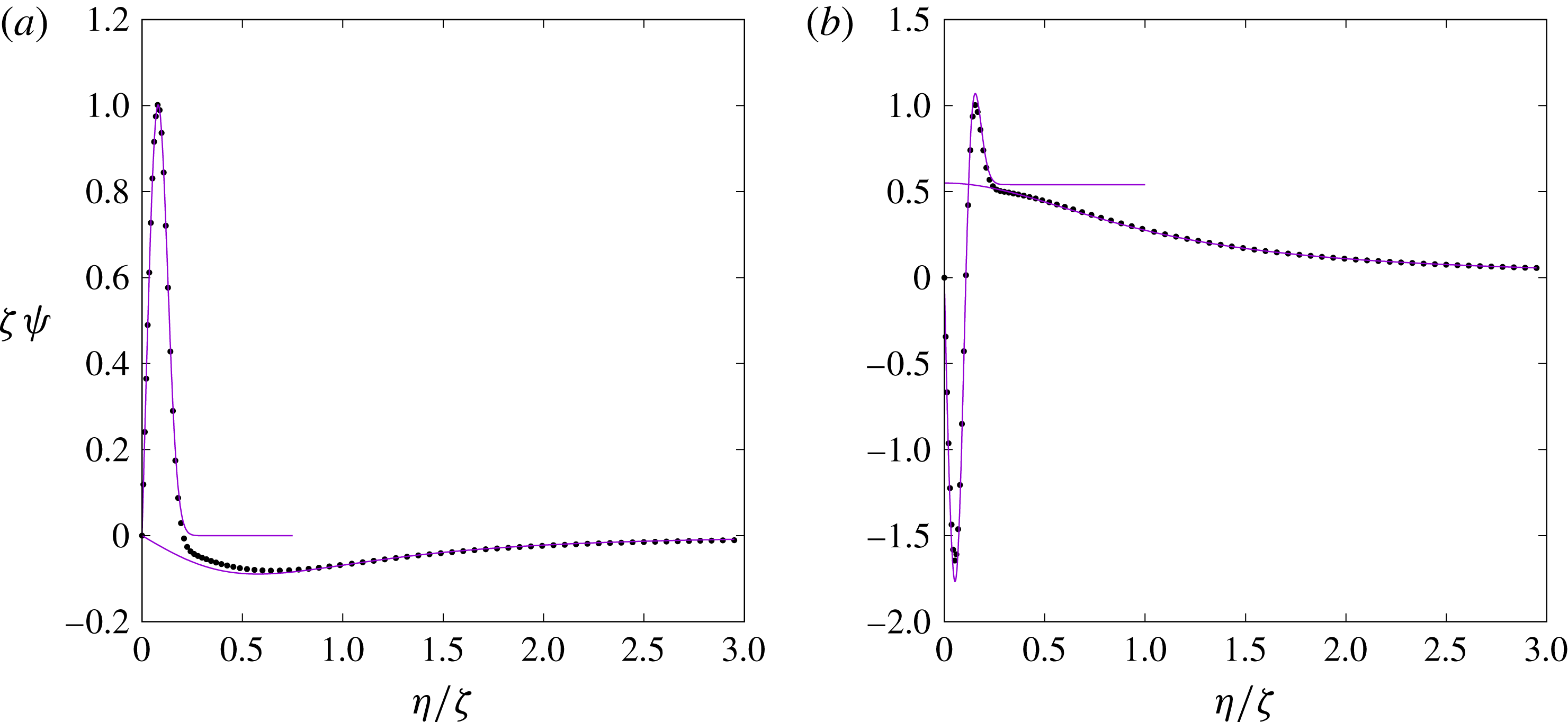
) shown in figure 1(a) with the predicted inner/outer descriptions of (2.5) and (2.9) respectively. Figure 2(a) shows this comparison for a cross-section of
 $\unicode[STIX]{x1D713}$
taken at
 $\unicode[STIX]{x1D701}=20$
, normalised such that the peak value is unity.
A comparison of the computed bi-global eigenmode data (points) with the far-field
 $\unicode[STIX]{x1D701}\gg 1$
asymptotic predictions (solid lines). The asymptotic prediction shows the inner solution given by (2.5) for
 $\unicode[STIX]{x1D702}=O(1)$
, and the outer solution given by (2.9) for
 $\unicode[STIX]{x1D702}=O(\unicode[STIX]{x1D701})$
. (a) A (normalised) cross-section of the first eigenmode shown in figure 1(a) at
 $\unicode[STIX]{x1D701}=20$
. (b) A (normalised) cross-section of the third eigenmode shown in figure 1(c) at
 $\unicode[STIX]{x1D701}=20$
.

2.2.2 Modes not linked to those of Libby & Fox (Reference Libby and Fox1963) and Luchini (Reference Luchini1996):
$h(\infty )\neq 0$

For the third mode i.e.
 $\unicode[STIX]{x1D706}=\unicode[STIX]{x1D706}_{3}$
we find that
 $a_{1}\neq 0$
in the outer-flow solution. In this case (2.10) shows that we should expect a non-zero cross-flow on the boundary with
 $\unicode[STIX]{x1D713}=O(1/\unicode[STIX]{x1D701})$
. We must therefore take
 $\unicode[STIX]{x1D6FD}=1$
(again) in (2.3), but with
 $h(\infty )=-a_{1}$
to ensure a leading-order matching between the wall layer and the outer solution. These forced solutions of (2.5) can be found for any value of
 $\unicode[STIX]{x1D706}$
, and on leaving the wall layer we also require that
 $d=a_{2}$
for consistency between (2.6) and (2.10a
).
A similar result follows for the second mode with
 $\unicode[STIX]{x1D706}=\unicode[STIX]{x1D706}_{2}$
. Numerical evidence in this case is that
 $a_{1}=a_{2}=0$
and
 $a_{3}\neq 0$
. The analysis follows in the same way, leading to a forced inner solution near to the boundary but this time the more rapid radial decay of the outer solution requires that
 $\unicode[STIX]{x1D6FD}=3$
in (2.3); this rapid decay is evident in figure 1(b).
Unlike eigenmodes corresponding to
 $\unicode[STIX]{x1D706}_{1}$
and
 $\unicode[STIX]{x1D706}_{4}$
, these states appear to be inherently global and
 $\unicode[STIX]{x1D706}$
is not determined solely from the far-field structure provided by (2.5). Nevertheless, we can still show that the computed bi-global eigenmodes are consistent with this asymptotic (
 $\unicode[STIX]{x1D701}\gg 1$
) description. Figure 2(b) compares a (normalised) cross-section of
 $\unicode[STIX]{x1D713}$
for the eigenmode shown in figure 1(c) with the inner solution that comes from solving (2.5), and the outer solution of (2.9). The forcing of the inner solution by a non-zero outer value of
 $\unicode[STIX]{x1D713}$
as
 $\unicode[STIX]{x1D702}/\unicode[STIX]{x1D701}\rightarrow 0$
is clearly shown in figure 2(b), in contrast to figure 2(a).
3 Nonlinear steady streak/roll states
To compute nonlinear states we undertake a parabolic marching of the full system (1.9) subject to a finite-amplitude disturbance. We choose to force the disturbance via a localised injection through the plate surface:
 $$\begin{eqnarray}\hat{V}(x,Y=0,Z)=\unicode[STIX]{x1D705}\hat{V}_{in}(x,Z).\end{eqnarray}$$
This ad hoc perturbation will force a streak response with an amplitude parameterised by
 $\unicode[STIX]{x1D705}$
, and results in the following modified boundary conditions for (1.9)
 $$\begin{eqnarray}\unicode[STIX]{x1D6F7}=-\sqrt{2x}\unicode[STIX]{x1D705}\hat{V}_{in},\quad \unicode[STIX]{x1D6E9}=\unicode[STIX]{x1D6F9}_{\unicode[STIX]{x1D702}}+\sqrt{2x}\unicode[STIX]{x1D705}\frac{\unicode[STIX]{x2202}\hat{V}_{in}}{\unicode[STIX]{x2202}\unicode[STIX]{x1D701}},\quad \text{on }\unicode[STIX]{x1D702}=0.\end{eqnarray}$$
This model is introduced as conceptually comparable to the experimental configuration of Asai et al. (Reference Asai, Minagawa and Nishioka2002), where a spatially localised streak is generated by a 5.5 mm (or 7.5 mm) (width) by 2.4 mm (height) mesh screen placed perpendicularly to the plate 500 mm from the leading edge. The (undisturbed) displacement thickness at this point is
 $\unicode[STIX]{x1D6FF}_{0}^{\ast }\approx 2.4~\text{mm}$
. If the downstream response of a perturbation to the Blasius flow is captured by (1.9) then we should also expect to be able to reproduce the general features of these experiments.
We choose a simple, localised disturbance for (3.1) of the form
 $$\begin{eqnarray}\hat{V}_{in}=(2x)^{-1/2}\text{e}^{-\unicode[STIX]{x1D6FE}(x-x_{0})^{2}}G(\unicode[STIX]{x1D701}),\end{eqnarray}$$
where
 $\unicode[STIX]{x1D701}=Z/(2x)^{1/2}$
is a spanwise coordinate measured relative to the local (transverse) length scale of the Blasius solution. This disturbance is localised around
 $x=x_{0}$
, with decreasing streamwise extent as
 $\unicode[STIX]{x1D6FE}$
increases. The
 $(2x)^{1/2}$
factor ensures that the spanwise extent of the disturbance and the amplitude are measured relative to the local Blasius base-flow properties. For the spanwise shape of the disturbance we choose
 $$\begin{eqnarray}G(\unicode[STIX]{x1D701})=\text{e}^{-c\unicode[STIX]{x1D701}^{2}}(1-2c\unicode[STIX]{x1D701}^{2}),\end{eqnarray}$$
where
 $c$
sets the spanwise length scale. To mimic the Asai et al. (Reference Asai, Minagawa and Nishioka2002) experimental configuration the polynomial term is included in (3.3b
) to ensure that there is no net mass flux into the boundary layer, that is
 $\int _{0}^{\infty }G(\unicode[STIX]{x1D701})\,\text{d}\unicode[STIX]{x1D701}=0$
.
Parabolic marching of (1.9) begins at
 $x=0$
from trivial initial conditions on account of (3.3) being negligible at the leading edge for the considered values of
 $x_{0}$
. A second-order (Crank–Nicolson) scheme is used to march the system with Newton iteration to handle the nonlinearity. At each
 $x$
-station and each Newton iteration we are left to solve a
 $4NM\times 4NM$
sparse system, where
 $N,M$
are the number of nodes in
 $\unicode[STIX]{x1D701},\unicode[STIX]{x1D702}$
associated with a (second-order) central-difference discretisation. Each sparse solve is performed using a direct parallel solver (Amestoy, Duff & L’Excellent Reference Amestoy, Duff and L’Excellent2000) and care is taken with respect to choices of
 $N$
,
 $M$
and the domain truncation of
 $\unicode[STIX]{x1D701},\unicode[STIX]{x1D702}$
. To reduce the number of degrees of freedom, the mesh of nodes is non-uniformly spaced in both directions, to allow a higher resolution in the neighbourhood of
 $\unicode[STIX]{x1D701}=\unicode[STIX]{x1D702}=0$
.
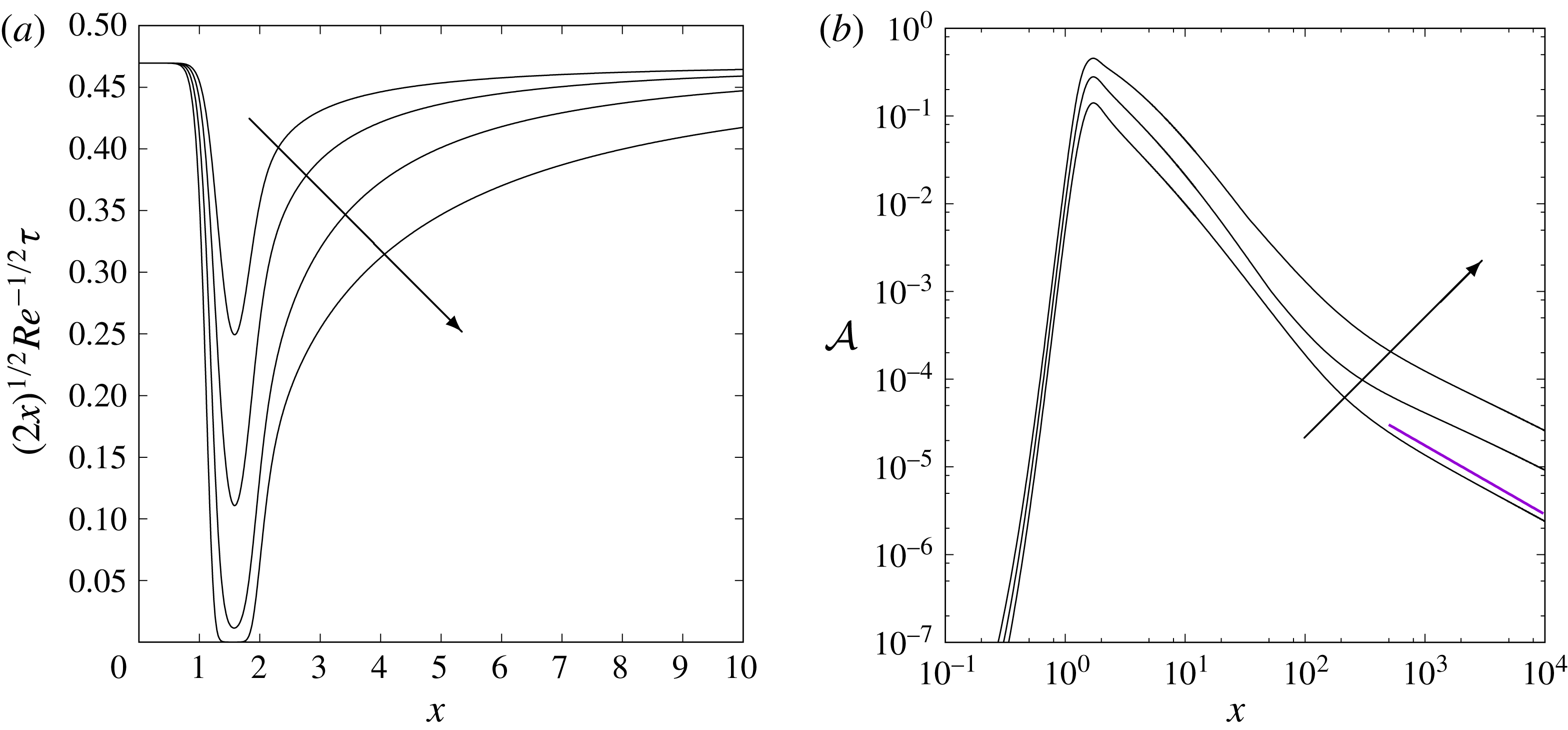
Solutions to (1.9) obtained by parabolic marching in the downstream coordinate
 $x$
. A localised injection given by (3.3) is imposed with
 $x_{0}=3/2$
,
 $\unicode[STIX]{x1D6FE}=10$
,
 $c=1/10$
, with
 $\unicode[STIX]{x1D705}$
increasing in the direction of the arrows shown. (a) The centreline shear rescaled such that the undisturbed Blasius base flow has a value of
 $0.4696\ldots$
and
 $\unicode[STIX]{x1D705}=1,2,4,8$
. (b) A global measure of the streak amplitude defined by (3.5) for
 $\unicode[STIX]{x1D705}=2,4,8$
. The line segment shows the predicted decay (
 $x^{\unicode[STIX]{x1D706}_{1}}$
) obtained from the linear (
 $\unicode[STIX]{x1D705}\ll 1$
) eigenvalue analysis of § 2.

To represent the downstream developing solution we examine the centreline (dimensionless) shear at the wall:
 $$\begin{eqnarray}\unicode[STIX]{x1D70F}(x)=u_{y}|_{y=0,z=0}=Re^{1/2}\hat{U} _{Y}|_{Y=0,Z=0}=Re^{1/2}(2x)^{-1/2}U_{\unicode[STIX]{x1D702}}|_{\unicode[STIX]{x1D702}=0,\unicode[STIX]{x1D701}=0}.\end{eqnarray}$$
We also present the global measure suggested by Andersson et al. (Reference Andersson, Brandt, Bottaro and Henningson2001)
 $$\begin{eqnarray}{\mathcal{A}}(x)={\textstyle \frac{1}{2}}\left[\max _{Y,Z}(\hat{U} -\hat{U} _{B})-\min _{Y,Z}(\hat{U} -\hat{U} _{B})\right],\end{eqnarray}$$
where
 $\hat{U} _{B}$
is the Blasius solution (
 $F^{\prime }$
in our earlier notation), so that
 $\hat{U} -\hat{U} _{B}=\tilde{U}$
in the notation of (1.8).
In figure 3(a) we show the evolution of the rescaled shear
 $\unicode[STIX]{x1D70F}(2x)^{1/2}Re^{-1/2}$
as a function of downstream distance
 $x$
, for an injection (3.3) with
 $\unicode[STIX]{x1D6FE}=10$
,
 $c=1/10$
,
 $x_{0}=3/2$
and increasing
 $\unicode[STIX]{x1D705}=1,2,4,8$
. It is worth noting that even for large-amplitude injection (
 $\unicode[STIX]{x1D705}=8$
) there is no evidence of any flow reversal and breakdown of the parabolic marching, instead the perturbation leaves a region of essentially zero shear until eventually starting to relax back towards the Blasius value of
 $0.4696\ldots \,$
. In the experimental work of Asai et al. (Reference Asai, Minagawa and Nishioka2002) it is also noted that there is no evidence of reverse flow behind the screen that provides the nonlinear disturbance mechanism.
A measure of the maximum disturbance to the streamwise velocity as measured by
 ${\mathcal{A}}$
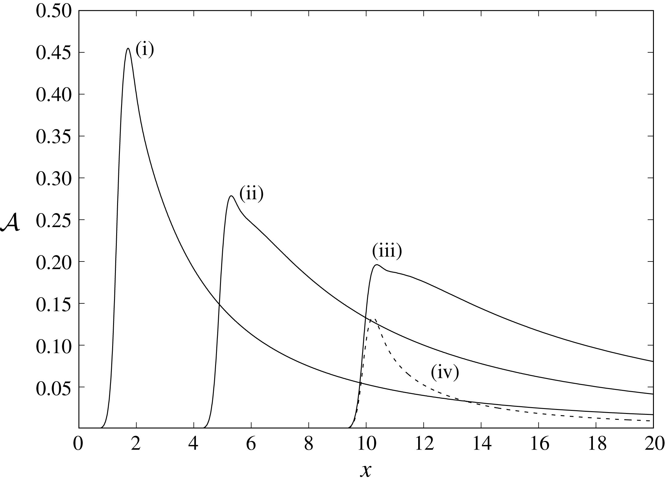
, defined by (3.5). The flow is perturbed nonlinearly via (3.1) with
 $\unicode[STIX]{x1D705}=8$
,
 $\unicode[STIX]{x1D6FE}=10$
. Four different cases are shown corresponding to (i)
 $x_{0}=3/2$
,
 $c=1/10$
, (ii)
 $x_{0}=5$
,
 $c=1/10$
, (iii)
 $x_{0}=10$
,
 $c=1/10$
and (iv)
 $x_{0}=10$
,
 $c=0.5$
.

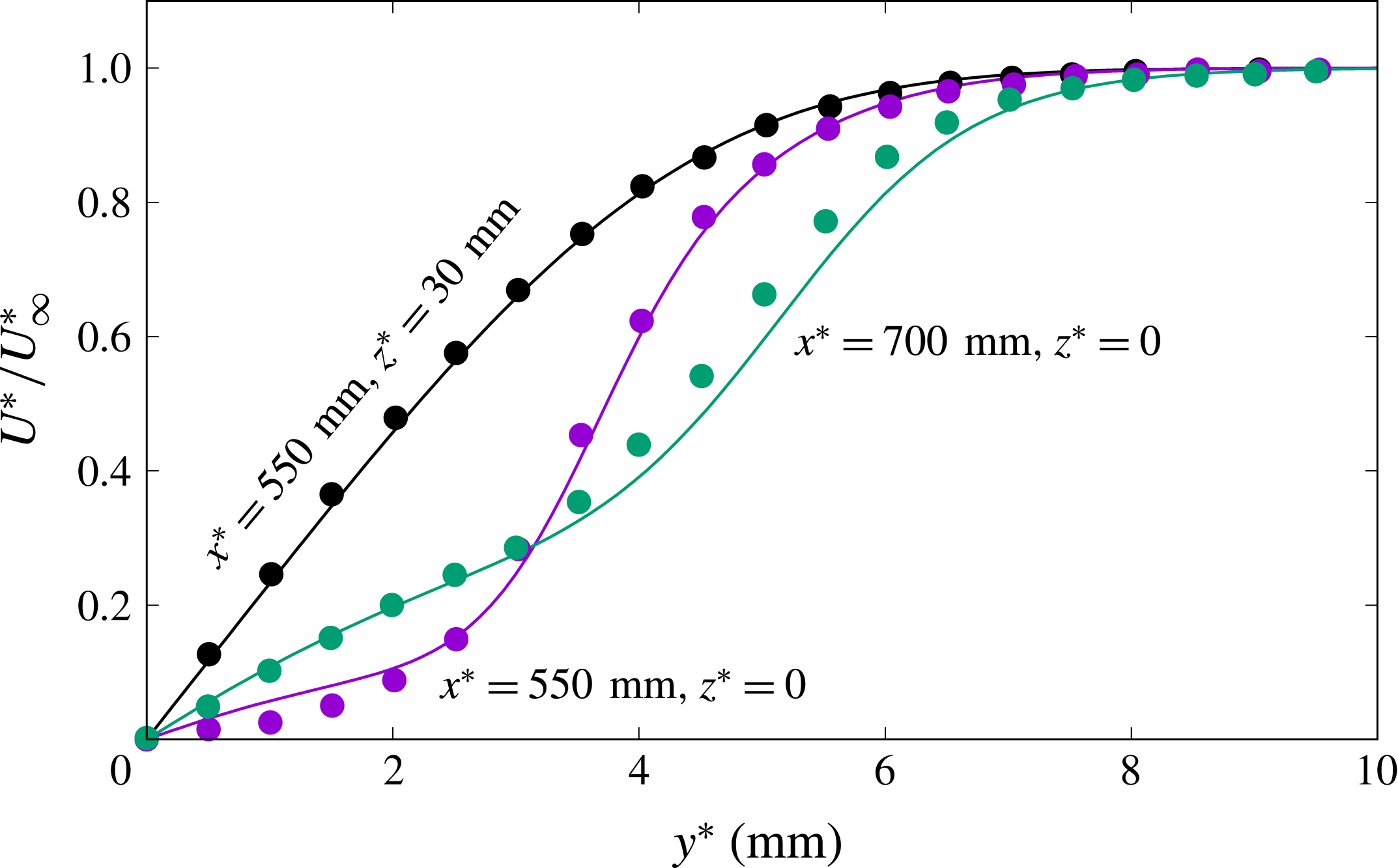
A solution of (1.9) subject to a perturbation of the form (3.1) (solid lines), compared to the (dimensional) experimental data (points) of Asai et al. (Reference Asai, Minagawa and Nishioka2002). The parameters in (3.3) are
 $\unicode[STIX]{x1D705}=12$
,
 $x_{0}=10$
,
 $\unicode[STIX]{x1D6FE}=10$
and
 $c=1/10$
; this choice of
 $x_{0}$
corresponds to choosing
 $L^{\ast }=5~\text{cm}$
in the non-dimensionalisation.

Figure 3(b) shows the evolution of
 ${\mathcal{A}}$
for the same disturbance with
 $\unicode[STIX]{x1D705}=2,4,8$
, but over a substantially longer downstream length scale. The perturbation is long lived, with an ultimate decay that is algebraic; the figure also shows the predicted least-damped decay rate of
 $x^{-0.787}$
that arises from the (linearised) bi-global eigenmode prediction of
 $\tilde{U} \sim x^{\unicode[STIX]{x1D706}_{1}}$
(as per table 1).
The impact of the disturbance location and spanwise extent, as parameterised by
 $x_{0}$
and
 $c$
in (3.3), is shown in figure 4. Increasing
 $x_{0}$
decreases the amplitude of the resulting disturbance, being effectively over a length scale (
 $1/\unicode[STIX]{x1D6FE}$
) that is reduced compared to the local boundary-layer length scale (which is growing as
 $\sqrt{x_{0}}$
). For larger values of
 $c$
the recovery towards a Blasius solution occurs over a shorter downstream distance. This is to be expected, as larger
 $c$
leads to a disturbance over a smaller spanwise length scale which in the nonlinear regime reduces more rapidly owing to spanwise diffusion. For more modest variations in the spanwise extent of the forcing, the streamwise centreline velocity of the streak is relatively insensitive. This is consistent with the experiments of Asai et al. (Reference Asai, Minagawa and Nishioka2002), which show only small-scale differences (at
 $z=0$
) when comparing the streaks generated by screens of width 7.5 mm and 5.5 mm.
A more quantitative comparison can be made with the available experimental data. To do this we take the data of Asai et al. (Reference Asai, Minagawa and Nishioka2002) for a 7.5 mm mesh screen, comparing the reported velocity profiles at the centre of the streak (
 $z=0$
) with numerical results. Clearly we cannot precisely model the nonlinear disturbance associated with this choice of mesh screen, and we have not taken any systematic approach to maximise the level of agreement. Nevertheless, a comparison is shown in figure 5 for
 $x_{0}=10$
,
 $\unicode[STIX]{x1D705}=12$
with our default values of
 $\unicode[STIX]{x1D6FE}=10$
and
 $c=1/10$
. (Given the self-similar nature of the Blasius base-flow one could of course equally choose
 $x_{0}=1$
,
 $\unicode[STIX]{x1D6FE}=100$
, for example.)
Given that the mesh screen disturbs the flow at
 $x^{\ast }=500\,\text{mm}$
in the experimental configuration, this corresponds to a choice of
 $L^{\ast }=\,50\,\text{mm}$
in our non-dimensionalisation with
 $Re\approx 13\,540$
. The comparison of figure 5 is shown in terms of the dimensional coordinate normal to the plate,
 $y^{\ast }$
. The profile far from the disturbance source (
 $z^{\ast }=30~\text{mm}$
) is clearly in agreement with an undisturbed Blasius profile. In the wake of the screen, two profiles are presented corresponding to
 $x^{\ast }=550~\text{mm}$
(
 $x=11$
) and
 $x^{\ast }=700~\text{mm}$
(
 $x=14$
). This comparison provides some encouragement that (1.9) can effectively model the downstream response, however we make no claims beyond consistency of the results given that the computation is not precisely replicating the experimental disturbance of the mesh screen.
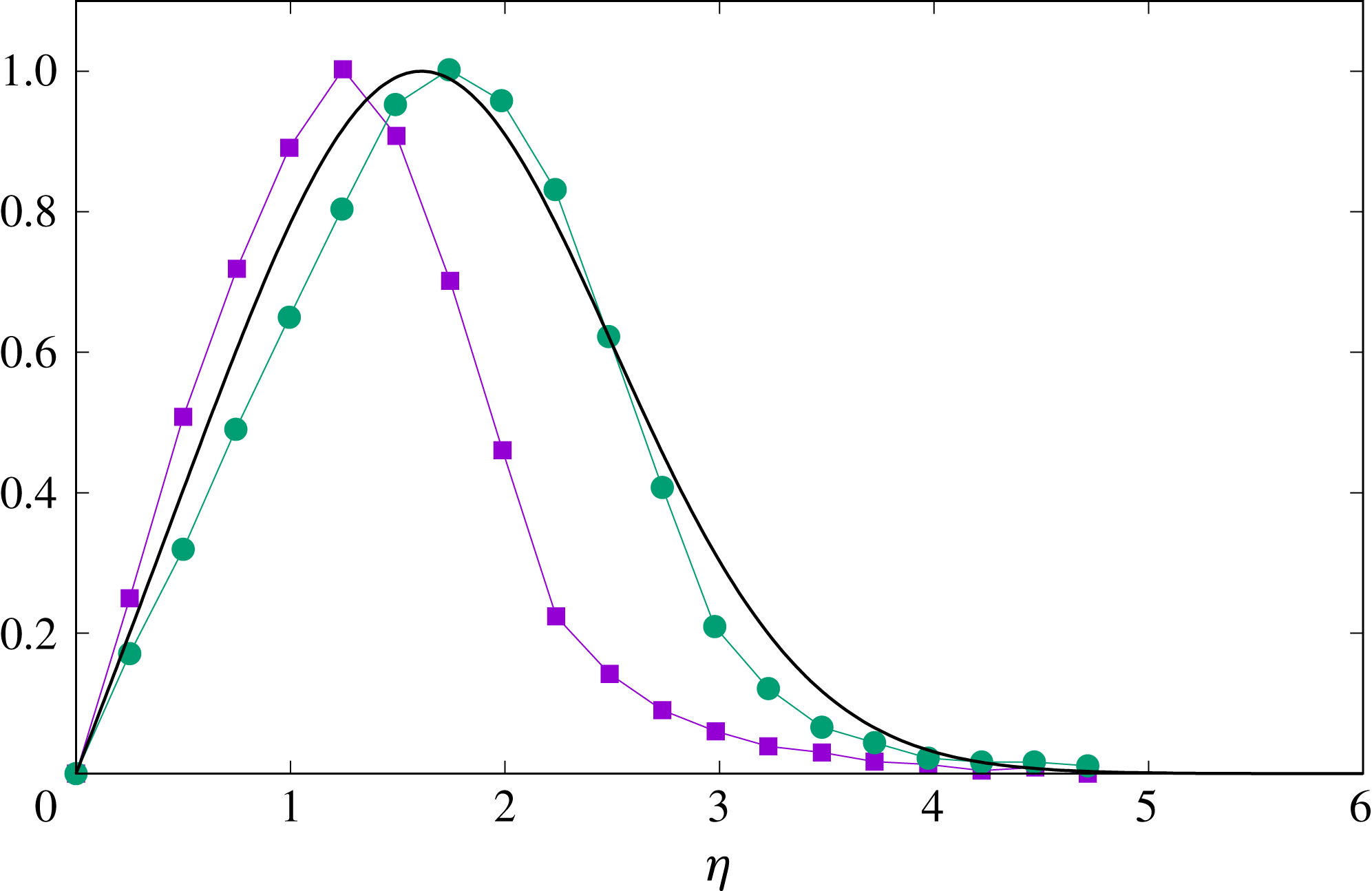
Normalised experimental data (points) of Asai et al. (Reference Asai, Minagawa and Nishioka2002) mapped to the non-dimensional coordinate
 $\unicode[STIX]{x1D702}$
. Data points show the (normalised) deviation from a Blasius profile along the streak centreline (
 $z=0$
, or equivalently
 $\unicode[STIX]{x1D701}=0$
). Squares/circles correspond to data acquired at
 $x^{\ast }=550~\text{mm}$
and 700 mm respectively. The solid line is obtained from the least-damped (
 $\unicode[STIX]{x1D706}_{1}$
) eigenmode shown in figure 1(a).

To remove the ambiguity of the disturbance generation mechanism, we also compare these same experimental results with the bi-global eigenmodes discussed in § 2. To do this we subtract the (experimentally obtained) velocity profiles in figure 5 from the appropriate Blasius solution at the two locations
 $x^{\ast }=550$
, 700 mm, to give a nonlinear perturbation to the streamwise velocity along
 $z=0$
. After normalising the perturbation to have a unit maximum velocity, and converting the dimensional transverse coordinate
 $y^{\ast }$
to the dimensionless value
 $\unicode[STIX]{x1D702}$
, we compare these data with the corresponding centreline perturbation of the least-damped eigenmode shown in figure 1(a). Despite the obvious nonlinear nature of the perturbation at
 $x^{\ast }=700~\text{mm}$
(as shown in figure 5), the normalised response compares favourably with the shape of the first linear mode. In this regard it is worth noting that the second mode very closely reproduces the shape of the first mode along the centreline, whilst the third mode is of the same shape but displaced to slightly larger values of
 $\unicode[STIX]{x1D702}$
.
4 Discussion
We have shown that for a Blasius base flow, the classical linearised (two-dimensional) modes of Libby & Fox (Reference Libby and Fox1963) can be generalised to give three-dimensional modes corresponding to self-similar perturbations that remain localised in the spanwise coordinate. These new linearised modes lead to a bi-global eigenvalue computation for the eigenmode velocity field, with the downstream algebraic decay rate being the eigenvalue. We show that the slowest-decaying localised streak perturbation behaves like
 $x^{\unicode[STIX]{x1D706}}$
, where
 $\unicode[STIX]{x1D706}=\unicode[STIX]{x1D706}_{1}\approx -0.787$
.
We have shown that a subset of our computed values for the eigenvalue
 $\unicode[STIX]{x1D706}$
can be related to those of Luchini (Reference Luchini1996), who effectively sought spanwise-periodic disturbances to the velocity components of the form
 $$\begin{eqnarray}\unicode[STIX]{x1D716}x^{\unicode[STIX]{x1D706}}\left(u(\unicode[STIX]{x1D702}),\frac{v(\unicode[STIX]{x1D702})}{(2x)^{1/2}},\frac{w(\unicode[STIX]{x1D702})}{2x}\right)\text{e}^{\text{i}kZ}\quad \text{with }\unicode[STIX]{x1D702}=Y/(2x)^{1/2}.\end{eqnarray}$$
However, progress for this approach was achieved by assuming a small spanwise wavenumber
 $k\ll 1$
, whilst
 $kw=O(1)$
. This small-wavenumber scaling for
 $w$
is crucial in order to retain three-dimensional effects and is equivalent to replacing periodicity in
 $Z$
with a cross-flow that is proportional to
 $Z$
. The governing equations of Luchini (Reference Luchini1996) are therefore also obtained for a disturbance of the form
 $$\begin{eqnarray}\unicode[STIX]{x1D716}x^{\unicode[STIX]{x1D706}}\left(u(\unicode[STIX]{x1D702}),\frac{v(\unicode[STIX]{x1D702})}{(2x)^{1/2}},\unicode[STIX]{x1D701}\frac{w(\unicode[STIX]{x1D702})}{(2x)^{1/2}}\right),\end{eqnarray}$$
where
 $\unicode[STIX]{x1D701}=Z/(2x)^{1/2}$
is a rescaled spanwise coordinate.
If we compare (4.2) to the algebraic decay of the localised eigenmode at large spanwise distances (
 $\unicode[STIX]{x1D701}\gg 1$
), as described by (2.3), we recover the same flow field for
 $\unicode[STIX]{x1D6FD}=-1$
. That the two problems are connected therefore reduces to the observation that the eigenvalue problem (2.5) can be applied to any algebraically varying spanwise perturbation simply by including the parameter
 $\unicode[STIX]{x1D6FD}$
in the streamwise decay rate via (2.7) and (2.8).
We have shown consistency between nonlinear streak states driven by boundary injection and the linearised eigenvalue analysis, by parabolic marching the governing system (1.9). Furthermore we can demonstrate favourable comparisons with limited available experimental data for localised streaks. We could no doubt improve these comparisons further, by fine tuning the parameters associated with the boundary injection, but since we cannot model the mesh screen disturbance employed in the experiments we choose not take this approach. We note that these experiments have also been similarly reproduced by unsteady three-dimensional Navier–Stokes calculations in the work of Brandt (Reference Brandt2007). However, the nonlinear boundary-region calculations can be carried out at a fraction of the cost of direct numerical simulations of the Navier–Stokes equations.
The formulation of the boundary-region equations is a fully rational process (i.e. their derivation can be fully justified on asymptotic consistency grounds). Indeed, they capture a good deal of the physics of the full Navier–Stokes system (lacking primarily only the streamwise pressure gradient and the streamwise viscous diffusive terms). It seems likely that this makes them robust and they certainly display a lack of singular behaviour otherwise often encountered in boundary-layer studies.
An interesting feature seen in our calculations (notably figure 3 a) is that even large disturbances do not seem to trigger flow reversal, an observation that appears to be consistent with the experimental results of Asai et al. (Reference Asai, Minagawa and Nishioka2002) as depicted in figure 5. Indeed, the authors have performed a number of other calculations using the boundary-region equations for other flow configurations (including results presented in Hewitt et al. (Reference Hewitt, Duck and Williams2017)), and this lack of flow reversal, even for significant flow disturbances, seems to be a common feature.
As we note in the introduction, streaks are well known to incite secondary instabilities and the framework of this current work is clearly open to a rational non-parallel approach to such viscous three-dimensional travelling disturbances.