Introduction
Coastal environments are subject to various processes and variables, and are constantly changing as they seek a dynamic equilibrium (Banikoi et al. Reference Banikoi, Schlüter and Manlosa2023; Wright and Thom Reference Wright and Thom2023). They play several vital roles, such as coastal protection, supporting recreational and tourism activities, and providing habitats for diverse species (Scheld et al. Reference Scheld, Bilkovic, Stafford, Powers, Musick and Guthrie2024; Virtanen et al. Reference Virtanen, Kallio, Nurmi, Jernberg, Saikkonen and Forsblom2023). These environments are highly dynamic and sensitive, continually receiving energy and material flows due to various natural processes, and they are also affected by human activities (Cruz-Ramírez et al. Reference Cruz-Ramírez, Chávez, Silva, Muñoz-Perez and Rivera-Arriaga2024; Priya et al. Reference Priya, Muruganandam, Sivarethiamohan, Sujatha, Madhava, Priya, Thirumala and Senthil2023). Human interventions have led to significant changes in the sediment balance along coastlines, causing losses, flow blockages, and even materials redistribution, which can result in imbalances within coastal ecosystems (Sahavacharin et al. Reference Sahavacharin, Sompongchaiyakul and Thaitakoo2022; Syvitski et al. Reference Syvitski, Angel, Saito, Overeem, Vörösmarty, Wang and Olago2022).
Coastlines are notably susceptible to impacts of global climate change, such as rising sea levels, and regional factors, such as alterations in wave patterns and storms (Griggs and Reguero Reference Griggs and Reguero2021; Pang et al. Reference Pang, Wang, Nawaz, Keefe and Adekanmbi2023). The primary driver of coastal plains formation in Brazil has been eustatic sea level changes linked to climate shifts (Suguio et al. Reference Suguio, Martin, Bittencourt, Dominguez, Flexor and Azevedo1985). Coastal plains provide critical evidence of sea level fluctuations, and chronological data, sedimentary structures, and microfossil analyses have been used to study the evolution of coastal environments during the Quaternary Period (Martins et al. Reference Martins, França, Seddique, Sial, Pessenda, Camargo, Valença, Santos and Barcellos2021; Silva et al. Reference Silva, Souza, Garcia, Dillenburg, Cancelli and Kuhn2021). The palaeoecological conditions of the Brazilian coastal plain have been extensively investigated through the study of microfossils (Lima and Parise Reference Lima and Parise2020; Lopes et al. Reference Lopes, Pereira, Caron, Ritter, Souza, Dillenburg, Barboza, Tatumi, Yee, Kinoshita and Baffa2021).
Research on the evolution and paleoenvironmental reconstruction of coastal areas using palynological techniques is vital for understanding vegetation changes, driven by climatic shifts or human activities (Glover et al. Reference Glover, George, Heusser and MacDonald2021) and variations in sea level (Cheng et al. Reference Cheng, Shu, Hao, Gao, Li, Yuan and Zou2023; Hao et al. Reference Hao, Ouyang, Zheng, Zhuo and Liu2020). In examining late Holocene conditions in Brazil, several studies have focused on how climatic variations affected vegetation dynamics during this period (Buso Junior et al. Reference Buso Junior, Pessenda, Mayle, Lorente, Volkmer-Ribeiro, Schiavo, Pereira, Bendassolli, Macario and Siqueira2019; Robinson et al. Reference Robinson, Souza, Maezumi, C_ardenas, Pessenda, Prufer, Corteletti, Scunderlick, Mayle, Blasis and Iriarte2018). In the state of Rio de Janeiro, most palaeoenvironmental research on vegetation dynamics has been conducted in bays (Coelho et al. Reference Coelho, Barth and Chaves1999; Bartholomeu et al. Reference Bartholomeu, Barros, Lopes, Barth and Vilela2014; Barreto et al. Reference Barreto, Freitas, Souza, Vilela, Barth and Baptista Neto2016, Reference Barreto, Freitas, Abuchacra, Fonseca, Melo and Baptista Neto2019; Guanabara and Sepetiba) coastal lagoons (Luz et al. Reference Luz, Barth and Silva2005, Reference Luz, Barth and Silva2010; Misumi et al. Reference Misumi, Barros, Vilela and Barth2018), and islands (Coe et al. Reference Coe, Ramos, Silva, Gomes, Sousa, Macario and Dias2018; Freitas et al. Reference Freitas, Barreto, Oliveira e Silva, Macedo Dias and Baptista Neto2022).
Dinoflagellate cysts offer insights into processes related to Quaternary palaeoenvironmental reconstructions in marine and coastal settings (Gu et al. Reference Gu, Chiessi, Zonneveld and Behling2018; Harland et al. Reference Harland, Polovodova Asteman, Morley, Morris, Harris and Howe2016; Pospelova et al. Reference Pospelova, Price and Pedersen2015). However, fossil records of these organisms in the coastal regions of Brazil remains relatively unexplored compared to the extensively studied continental shelf and slope regions (Santos et al. Reference Santos, Carvalho, Oliveira and Filho2017; Souza et al. Reference Souza, Carvalho, Escamilla, Barreto, Freitas, Silva and Baptista Neto2020). From the correlation and interpretation of terrestrial and marine palynomorph data, it is possible to reconstruct regional/local vegetation as well as changes in the coastal environment. Pollen types in these environments can provide a view of the different vegetation gradients found in these locations together with a more regional or local view of their drainage basin, contributing to palaeoecological studies (Sanchez Goñi Reference Sanchez Goñi2022). On the other hand, dinoflagellate cysts are good ecological indicators (Sala-Pérez et al. Reference Sala-Pérez, Lattuada, Flecker, Anesio and Leroy2020) that are used in palaeoclimatic reconstructions and as indicators of marine palaeoproductivity (Dale & Fjellså, Reference Dale, Fjellså, Zahn, Pedersen, Kaminski and Labeyrie1994; Over and Pospelova Reference Over and Pospelova2022). Despite previous work in Brazilian coastal plains, no study has combined terrestrial and marine palynomorph analyses with 14C dating in Paraty. Given this, the main objective of the present work was to document and interpret palaeoenvironmental dynamics in the coastal plain of Paraty during the Holocene through analysis of terrestrial and marine microfossils associated with sea level variations.
Study area
The municipality of Paraty is located on the southern coast of Rio de Janeiro, bordered to the east by the city of Angra dos Reis and to the west by Ubatuba in São Paulo, and it is located between 23°13′21″S and 44°42′50″W. This region is a hotspot with high biodiversity. The Paraty geology features rocky areas with varying slopes, narrow coastal plains, and a range of beaches with different morphologies and sediment types, including sands and gravels (Pinheiro et al. Reference Pinheiro, Silva and Baptista Neto2021a). The rocky coast primarily consists of granites and gneisses, often displaying folds and faults (Guerra et al., Reference Guerra, Bezerra, Jorge and Fullen2013; Faria Reference Faria2018). Sediment input from small rivers and channels is significant along this coastline, with materials being transported from slopes and deposited on beaches (Carvalho et al. Reference Carvalho, Anjos, Veiga and Macario2011; Pinheiro et al. Reference Pinheiro, Silva and Baptista Neto2021a; Silva et al. Reference Silva, Gralato, Brum, Silvestre, Baptista and Pinheiro2020).
The overall water circulation in the area is influenced by the Brazil Current (BC), which flows from north to south along the Brazilian shelf and shelf slope. The atmospheric South Atlantic Subtropical Anticyclone (SASA), causes Ekman transport generating seasonal upwelling along the coast and shelf of Rio de Janeiro. This leads to the emergence of cold, eutrophic South Atlantic Central Water (SACW) (Kjerfve et al. Reference Kjerfve, Dias, Filippo and Geraldes2021). Between 7000 and 5000 yr BP, South America was also influenced by the South American Monsoon System (SAMS) (Prado et al. Reference Prado, Wainer, Chiessi, Ledru and Turcq2013) which resulted in intense humid conditions on the continent during austral summer and dry conditions during austral winter (Zhou and Lau Reference Zhou and Lau1998).
The Paraty region has a humid tropical climate without a water deficit, with an average annual rainfall of 2000 mm (Soares et al. Reference Soares, Francisco and Senna2014), a mean salinity ranging from 21 to 35 ppm (Kjerfve et al. Reference Kjerfve, Dias, Filippo and Geraldes2021), and a mean annual temperature of 22.5°C (Bittencourt and Rocha Reference Bittencourt and Rocha2002). The main vegetation along the Paraty coast is part of the Atlantic Forest biome, which is classified as a low-montane ombrophilous forest, associated with “restinga” forest (floristic composition observed in coastal sandy deposits), and mangrove areas. Important plant families in the region include Arecaceae, Nyctaginaceae, Clusiaceae, Myrtaceae, Elaeocarpaceae, Fabaceae, and Lauraceae, as well as Euphorbiaceae and Bignoniaceae (Borges and Peixoto Reference Borges and Peixoto2009; Assis et al. Reference Assis, Prata, Pedroni, Eisenlohr, Martins, Santos, Tamashiro, Alves, Vieira, Piccolo, Martins, Camargo, Carmo, Simões, Matinelli and Joly2011).
Materials and methods
Sediment core collection and laboratory analysis
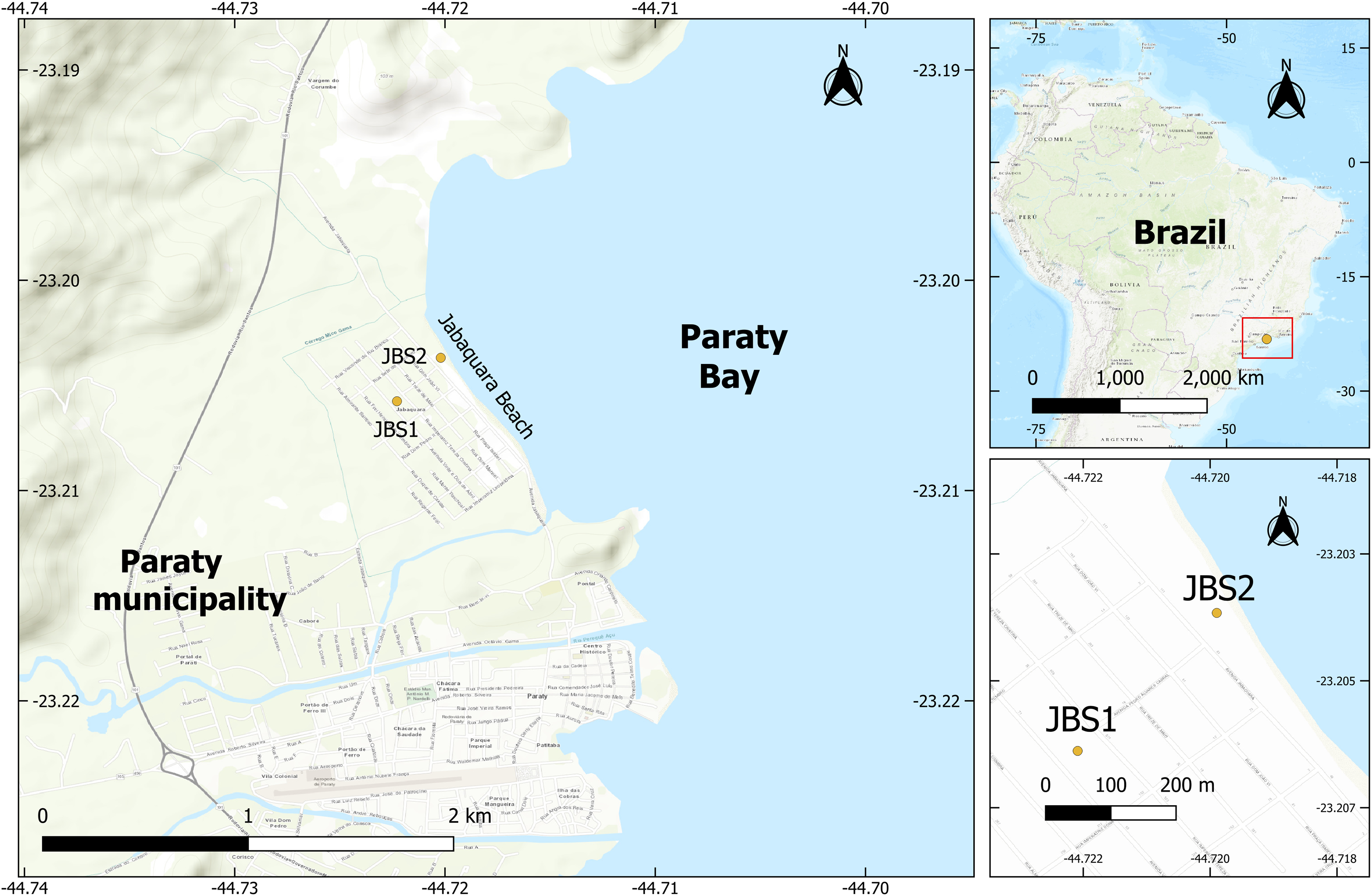
Two sediment cores were collected on the coastal plain of Paraty at coordinates JBS1 (44°43′20.22″W 23°12′20.70″S), 300 m from Jabaquara beach, and JBS2 (44°43′ 12.72″W 23°12′13.26″S) within Jabaquara beach (Figure 1). Coring was made using a mechanical device with PVC liner that reached depths of between 6 and 9 m. The sediment cores were subsequently inspected and sampled for particle size analysis, color description and micropaleontological analysis.
Location map of the two sediment core collection points in the Paraty coastal plain, Rio de Janeiro State, Brazil.

Figure 1 Long description
The map displays the Paraty coastal plain in Rio de Janeiro State, Brazil, highlighting two sediment core collection points labeled JBS1 and JBS2. The main map focuses on the Paraty municipality and bay, with JBS1 and JBS2 marked near Jabacuara Beach. An inset map shows the broader context within Brazil, indicating the specific region where the study area is located. Another inset provides a detailed view of the immediate vicinity around JBS1 and JBS2. The maps use various shades of blue to represent water bodies and different shades of beige to represent land features. The coordinates and scale bars help in understanding the precise locations and distances.
Particle size analysis
The pretreatment involved the removal of salt from the samples with distilled water. The mud fractions were analysed with a laser granulometer. Coarse sediments were analysed using the sieving method which consists of using different sieves of different mesh openings that are stacked to separate the grains of coarse sediments by size classes. The granulometric classification of the sediments was defined on the basis of Wentworth (Reference Wentworth1922). To describe the sediment color, a dry sample and a Munsell chart (Munsell Color 2010) were used.
14C-AMS dating
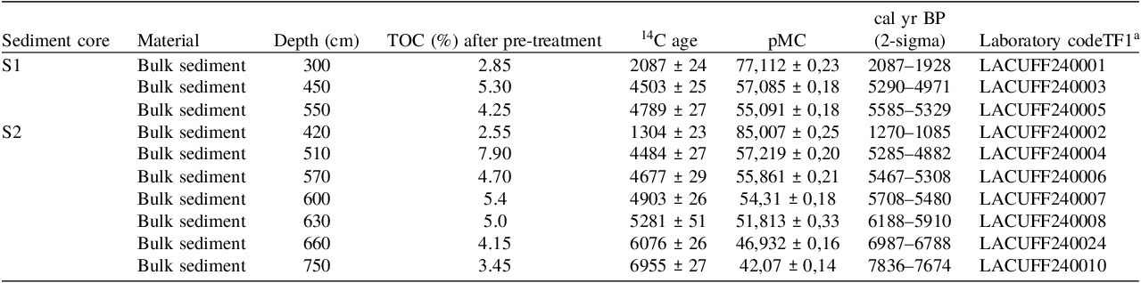
Eleven bulk sediment samples from the two sediment cores (JBS1 and JBS2) were selected for radiocarbon dating using the accelerator mass spectrometry (AMS) 14C method based on their TOC values (Table 1). In areas where a higher percentage of coarser grain size was identified, dating was not conducted due to the low or non-existent TOC percentage. Preliminary treatments for sediments followed the standard laboratory procedure that consists of repeated acid treatments to remove contaminants. Samples are exposed to 1.0 M hydrochloric acid (HCl) at 90°C for 2 hr, with treatments repeated until the supernatant becomes clear. If the procedure cannot be completed within a single day, samples are stored overnight in 0.1 M HCl at room temperature. Upon completion of the chemical pretreatment, the sediment is rinsed a minimum of five times with Milli-Q water and dried in an oven at 80°C. Careful control of the number of acid treatments is essential, as the required number of HCl cycles depends on the sediment type. While the acid effectively removes modern carbon from the sample, excessive acid exposure may also result in the loss of the target carbon fraction (Oliveira et al. Reference Oliveira, Macario, Carvalho, Moreira, Alves, Chanca, Diaz, Jou, Hammerschlag, Netto, Oliveira, Assumpção and Fernandes2021).
Sediment core samples dated by radiocarbon method collected in the coastal plain in Paraty, Rio de Janeiro State, Brazil

Table 1 Long description
The table presents data on sediment core samples dated using the radiocarbon method in Paraty, Rio de Janeiro State, Brazil. It includes information on sediment core identifiers, material type, depth in centimeters, total organic carbon percentage after pre-treatment, radiocarbon age, percentage of modern carbon, calibrated years before present, and laboratory code. The table has eleven rows and nine columns, detailing specific values for each sample. Notable trends include varying total organic carbon percentages and radiocarbon ages across different depths and sediment cores.
a LACUFF Laboratory
The organic carbon is converted into CO2 by combustion at 900°C for 3 hr in vacuum-sealed ampoules containing cupric oxide and silver. The resulting CO2 was cryogenic purified under vacuum by thermal water traps and then cryogenicall transferred by liquid-nitrogen trap into a graphitization tube. The graphitization process was carried out in vacuum-sealed ampoules containing titanium-hydride (TiH2) and zinc at 550°C, as described by Macario et al. (Reference Macario, Alves, Moreira, Oliveira, Chanca, Jou and Diaz2017). The resulting graphite was sent to the Center for Applied Isotope Studies (CAIS) at the University of Georgia, USA, for the measurement of carbon isotope ratios. These measurements were normalized using the National Bureau of Standards oxalic acid standard (SRM 4990c), and the 13C/12C ratio was corrected on the basis of accelerator measurements and indicated a continental organic carbon. The age model was constructed from the 14C-AMS dating of eleven sediment samples from two cores (JBS1 and JBS2). The analyses were conducted at the Radiocarbon Laboratory of the Federal Fluminense University (LAC-UFF), Brazil. Calibrated ages (BP) were determined using the Oxcal v.4.4.4 software and the Southern Hemisphere atmospheric calibration curve (SHCal20) (Hogg et al. Reference Hogg, Heaton, Hua, Palmer, Turney, Southon, Bayliss, Blackwell, Boswijk, Ramsey, Pearson, Petchey, Reimer, Reimer and Wacker2020) (Table 1).
Palynomorph sample preparation
For the pollen and dinocyst analyses, sediment cores were sampled at 10-cm intervals, with each sample weighing 2 g. The samples were subjected to chemical treatments following the standard methods of Faegri and Iversen (Reference Faegri and Iversen1989) with the acidification of the samples using HCl to remove carbonates and HF to remove silicates. Pollen samples were subjected to acetolysis (Erdtman Reference Erdtman1960); however this approach was not used for dinocyst sample analysis to prevent damage to the dinocysts from recent sediments (Pound et al. Reference Pound, O’Keefe and Marret2021). Dinocysts were recovered by filtering the residue through a 10 µm sieve mesh (Mertens et al. Reference Mertens, Bradley, Takano, Mudie, Marret, Aksu, Hiscott, Verleye, Mousing and Smyrnova2012), while ZnCl2 (density = 2) was used to float the organic parts (pollen and spores). To aid in the concentration calculations, each sample was spiked with one tablet of exotic Lycopodium clavatum spores, which contained 11,670 spores (Stockmarr Reference Stockmarr1971). Pollen grains were identified using various reference catalogues (Barreto et al. Reference Barreto, Freitas, Vilela, Neto and Barth2013; Colinvaux et al. Reference Colinvaux, De Oliveira and Patiño1999; Roubik and Moreno Reference Roubik and Moreno1991), and dinocysts were identified with standard reference catalogues (Lewis et al. Reference Lewis, Rochon and Harding1999; Matsuoka and Fukuyo Reference Matsuoka and Fukuyo2000; Radi et al. Reference Radi, Pospelova, de Vernal and Barrie2007; Rochon et al. Reference Rochon, de Vernal, Turon, Mathiessen and Head1999; Zonneveld and Pospelova Reference Zonneveld and Pospelova2015). Palynomorph percentages and concentrations were calculated, and TILIA and CONISS software programs (Grimm Reference Grimm1987) were used for graphing and statistical analysis, respectively. CONISS was specifically used for cluster analysis and zonation, wich was based on raw data from pollen grains and dinocysts, within a stratigraphically constrained framework.
Results
14C-AMS dating
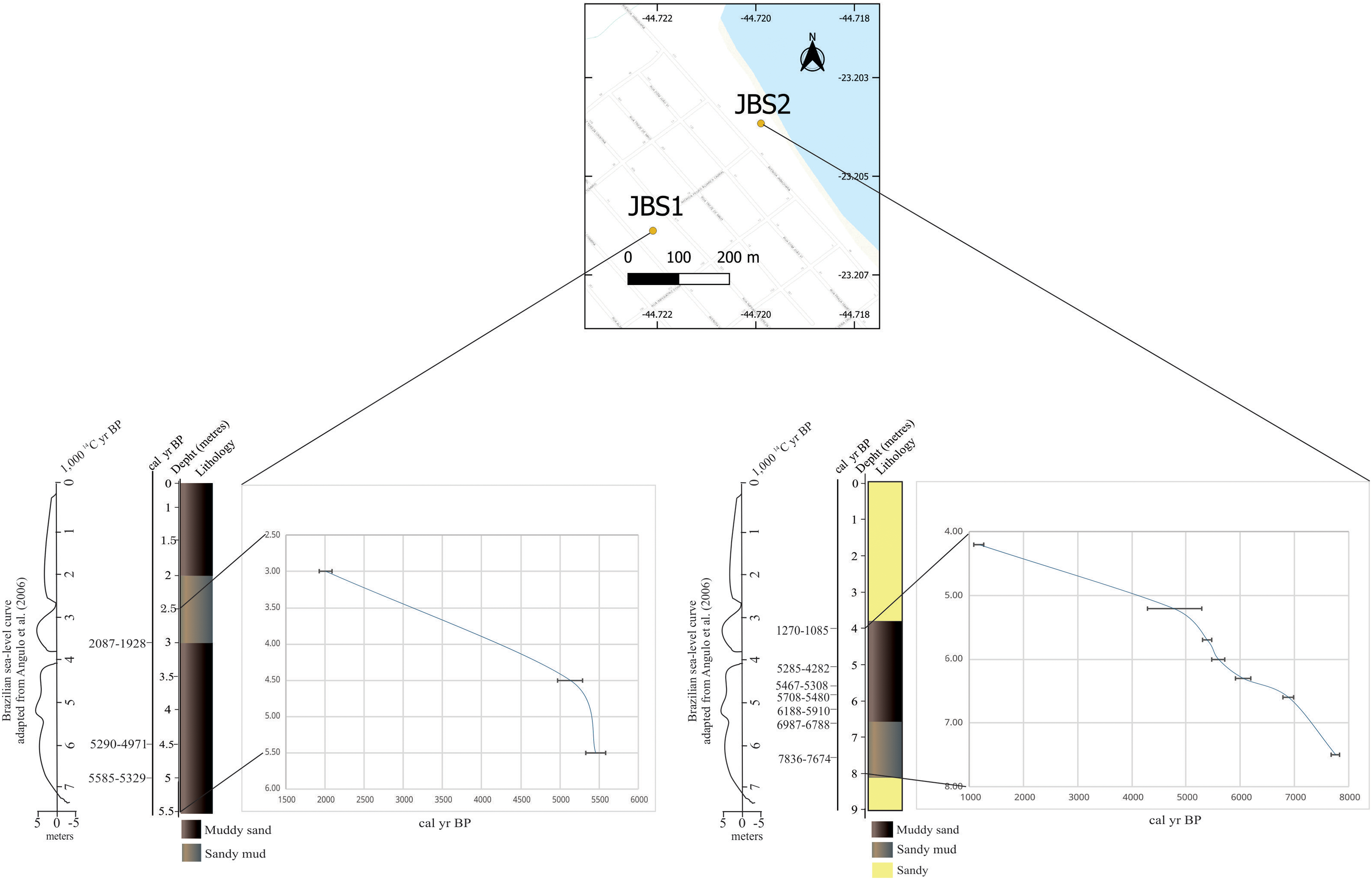
The results for the 11 dated samples are presented in Table 1 and Figure 2. The oldest age for JBS1 was obtained at a depth of 550 cm (5585–4282 cal yr BP). The JBS2 sediment core give the oldest age at 750 cm depth (7836–7674 cal yr BP). The youngest dates were observed at 300 cm depth (2087–1928 cal yr BP) in the JBS1 sediment core (Figure 3) and 1270–1085 cal yr BP in the JBS2 sediment core (Figure 4). Sedimentation rates varied across the cores. In JBS1, the mid Holocene interval (550–450 cm) shows an estimated accumulation rate of 0.31 cm/yr, decreasing to 0.05 cm/yr during the late Holocene (450–300 cm). In JBS2, the interval at 750–660 cm core depth recorded a rate of 0.10 cm/yr, with a progressive decline to 0.04–0.03 cm/yr in the overlying sections at 660–630 cm and 630–600 cm, respectively. A temporary increase occurred between 600 and 570 cm, with rates reaching 0.28 cm/yr before decreasing to 0.09 cm/yr and further down to 0.03 cm/yr in the uppermost dated intervals. The average sedimentation rate estimated for core JBS1 is approximately 0.14 cm/yr. For JBS2 sediment core, the average sedimentation rate is lower, around 0.07 cm/yr.
Chronological model for sediment cores JBS1 and JBS2 collected in the Paraty region.

Figure 2 Long description
The image contains two sediment core graphs labeled JBS1 and JBS2, collected in the Paraty region. Each graph displays sediment depth in meters on the y-axis and calibrated years before present (cal yr BP) on the x-axis. The graphs include sedimentology information, with muddy sand and sandy mud layers indicated by different colors. The Brazilian sea level curve is adapted from Angulo et al. (2006) and shown alongside the sediment core data. The graphs illustrate the depth and age of sediment layers, providing insights into the chronological model of the sediment cores. All values are approximated.
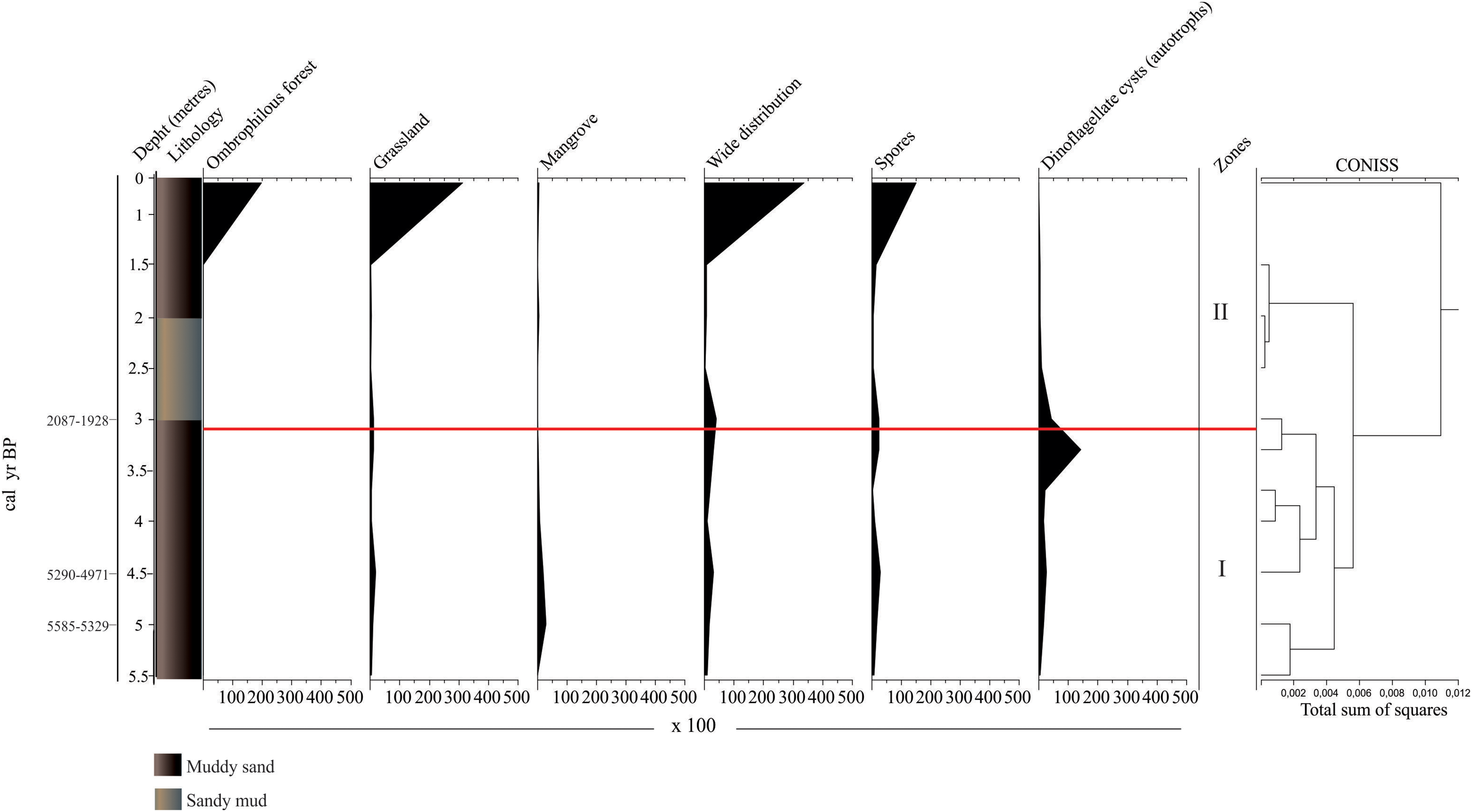
Pollen types (pollen/g) and dinoflagellate (cysts/g) concentrations observed in the JBS1 sediment core collected in the Paraty region.

Figure 3 Long description
The line graph illustrates the concentrations of pollen types and dinoflagellate cysts in the JBS1 sediment core collected in the Paraty region. The x-axis represents the depth in centimeters, ranging from 0 to 550 centimeters. The y-axis represents the calibrated years before present (cal yr BP), ranging from 0 to 5585 years. The graph includes multiple panels showing different variables: depth in meters, lithology, vegetation types such as ombrophilous forest, grassland, mangrove, and wide distribution, as well as spores and dinoflagellate cysts. The lithology is indicated by colors: muddy sand and sandy mud. The zones are divided into two sections, labeled as 2 and 1, with a red horizontal line marking a significant boundary at approximately 3000 cal yr BP. The total sum of squares is shown in a dendrogram on the right side of the graph. All values are approximated.
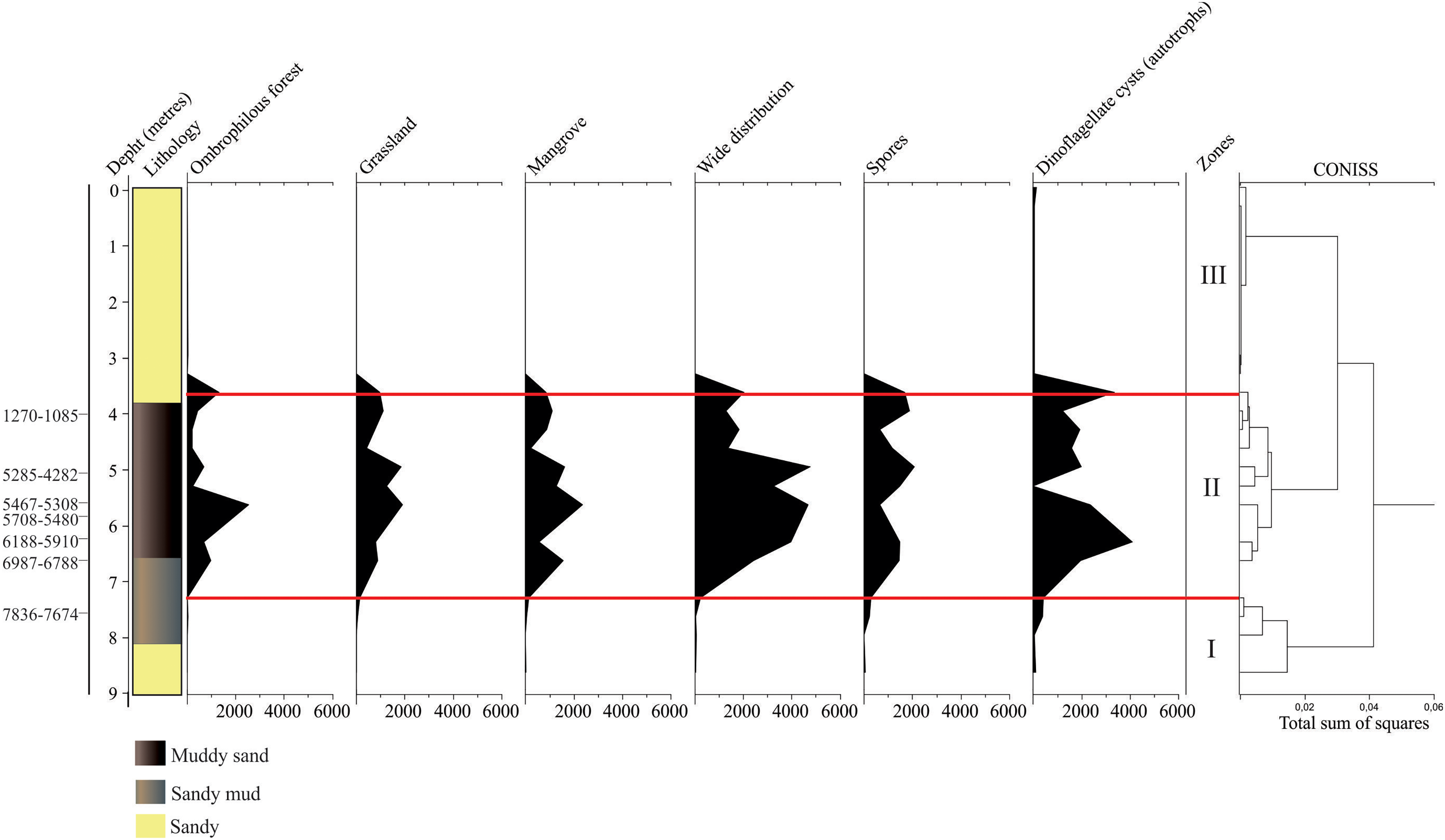
Pollen types (pollen/g) and dinoflagellate (cysts/g) concentrations observed in the JBS2 sediment core collected in the Paraty region.

Figure 4 Long description
The line graph presents data on pollen types and dinoflagellate concentrations observed in the JBS2 sediment core collected in the Paraty region. The x-axis represents the depth in meters, ranging from 0 to 9 meters. The y-axis represents the concentration of pollen and dinoflagellate cysts in grams per liter, ranging from 0 to 7000. The graph is divided into several columns, each representing different types of pollen and dinoflagellate cysts, such as lithophylous forest, ombrophylous forest, grassland, mangrove, wide distribution, spores, and dinoflagellate cysts. The sediment core is categorized into three zones, labeled I, II, and III, based on the total sum of squares. The sediment types are color-coded: muddy sand, sandy mud, and sandy. The graph shows variations in concentrations at different depths, with notable peaks and troughs indicating changes in pollen and dinoflagellate cyst levels over time. All values are approximated.
Sediment characteristics
Sediment core JBS1 is a moderately sorted deposit consisting predominantly of mud, varying-between sandy silt and silty sand. The sediment color is predominantly grey (grey 1 2.5/10GY), except at the top, which is black (10YR 2/1 black) indicating a sediment with low iron presence and organic matter (gray) and high organic matter content (black) (Munsell Color, 2010; Suguio, Reference Suguio2003). Sediment core JBS2 is poorly sorted, varying from sand to sandy silt. The sediment colors range from grey tones at the base to 4.2 m (2.5Y 7/2 light grey; 2.5Y 6/1 grey; 10Y 5/1 greenish grey), and the brown tones ranged from 3.9 m to the surface (10YR 5/3 brown; 10YR 4/6 dark yellowish brown; 2.5Y 6/4 light yellowish brown) indicating a low iron presence (gray, greenish gray), with a moderated organic matter content and iron oxidation (brown) (Figures 3 and 4).
Terrestrial palynomorphs
In sediment core JBS1, 10 pollen types from 10 botanical families were identified. A greater concentration of pollen types was observed near the top of the sediment core (Figure 3). In core JBS2, 19 pollen types were identified, covering 16 botanical families. The most representative vegetation was Ombrophilous forest (Figure 4). From the analysed samples, it was possible to group the identified pollen types into four vegetation types (Ombrophilous forest, grassland, mangrove and wide distribution) on the basis of specific bibliographies. Pollen types that occurred in more than one set of plants were classified as taxa with a “wide distribution” (Figures 5 and 6). Zones were subsequently established for each sediment core with the aid of CONISS.
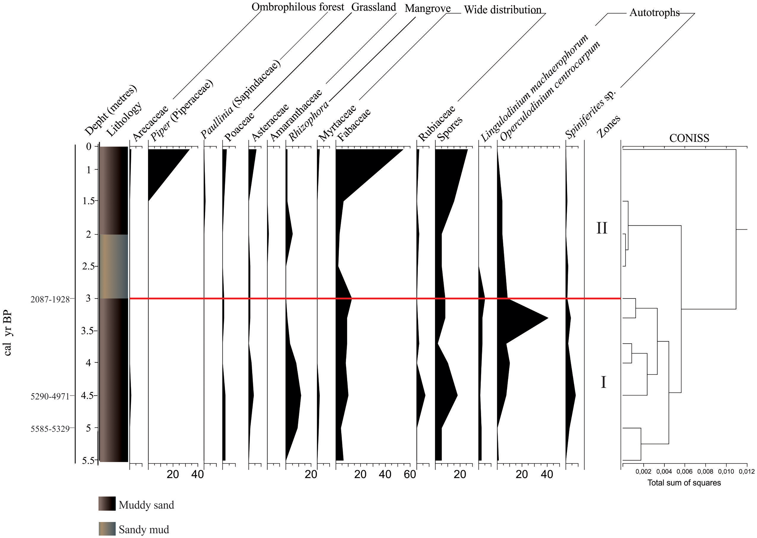
Pollen types and dinoflagellate cyst frequencies (%) observed in the JBS1 sediment core collected in the Paraty region.

Figure 5 Long description
The line graph presents the pollen types and dinoflagellate cyst frequencies observed in the JBS1 sediment core collected in the Paraty region. The x-axis represents the depth in meters, ranging from 0 to 5.5 meters, while the y-axis represents the percentage of pollen types and dinoflagellate cysts, ranging from 0 to 60 percentage. The graph includes various pollen types such as Arecaceae, Piper, Paulinia, and others, as well as dinoflagellate cysts like Lingulodinium machaerophorum and Operculodinium centrocarpum. The sediment core is divided into two zones, I and II, with a red line marking a significant boundary at approximately 3 meters depth. The lithology column on the left indicates the sediment composition, with muddy sand and sandy mud layers. The dendrogram on the right shows the clustering of the data into zones based on the total sum of squares. All values are approximated.
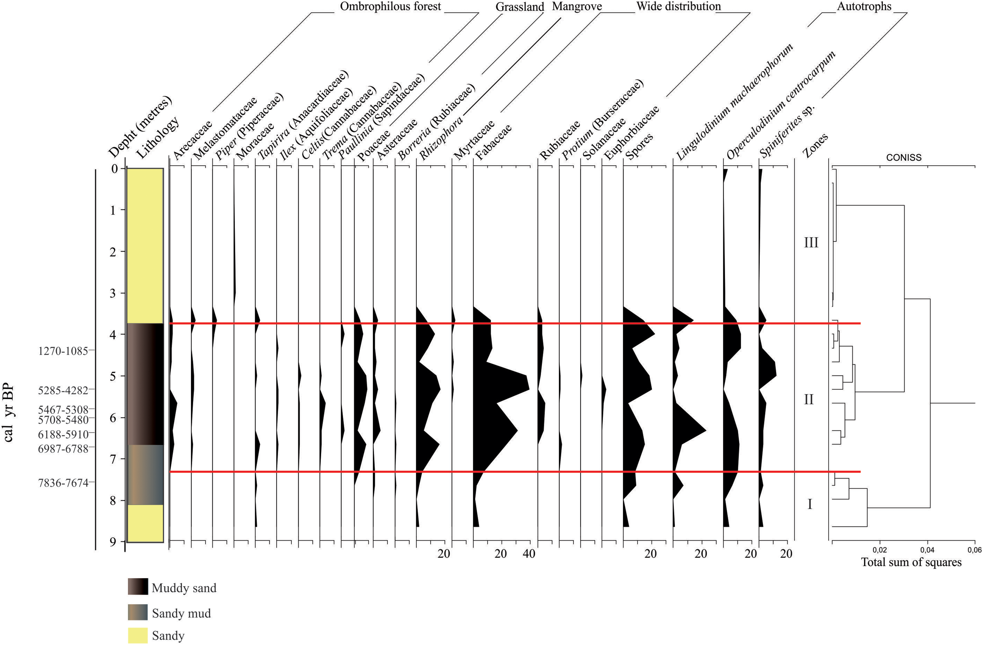
Pollen types and dinoflagellate cyst frequencies (%) observed in the JBS2 sediment core collected in the Paraty region.

Figure 6 Long description
The line graph presents data on pollen types and dinoflagellate cyst frequencies observed in the JBS2 sediment core collected in the Paraty region. The x-axis represents depth in meters, ranging from 0 to 9 meters. The y-axis represents calibrated years before present (cal yr BP), ranging from 0 to 7836-7674 years. The graph includes various pollen types and dinoflagellate cysts, categorized by lithology: muddy sand, sandy mud, and sandy. The graph is divided into three zones: I, II, and III, with specific pollen types and cysts highlighted. The data points show fluctuations in frequencies across different depths and time periods. All values are approximated.
Marine palynomorphs
In the two sediment cores three species of dinoflagellates (Lingulodinium machaerophorum, Operculodinium centrocarpum and Spiniferites sp.) were found, all of which are considered autotrophic organisms. In the JBS1 sediment core, the highest concentration values were observed at depths of 4.5 m (2606 cysts/g), 3.3 m (14296 cysts/g) and 3.0 m (4292 cysts/g) m (Figure 3). In the JBS2 sediment core, the highest accumulation rate occurred at a depth of 6.6 m (4079 cysts/g) (Figure 4).
Description of the JBS1 sediment core
Zone I – (5.5 to 3.1 m depth)
This zone is characterized by a low total concentration of palynomorphs. The most expressive vegetal formation in this zone was the “wide distribution” type (3,986 pollen/g) at 3.1 m depth (Figure 3). In this zone, Rhizophora and Fabaceae were the pollen types that presented the highest frequency (Figure 5). Dinoflagellate cysts had low concentration values from the base of the sediment core up to 3.3 m depth where the highest value of the entire sediment core was observed (14,296 cysts/g) (Figure 3).
Zone II – (3.1 m to 0 cm depth)
This zone presents low accumulation of palynomorphs, with an increase in concentration observed from 1.5 m depth with a progressive increase towards the top of the core for all plant formations including the spores (Figure 3). In this zone, Piper and Fabaceae stood out as the most frequent pollen types (Figure 5). Dinoflagellate cysts are present with low concentration of cysts within this zone (Figure 3).
Description of the JBS2 sediment core
Zone I – (9 to 7.3 m depth)
Within this zone low concentrations of palynomorphs are observed. Increased accumulation was observed from 7.5 m core depth, with a progressive increase towards the core top for all the plant formations, including the spores (Figure 4). In this zone, Piper and Fabaceae were the most common pollen types found (Figure 6). Dinoflagellate cysts had low concentration values in this zone (Figure 4).
Zone II – (7.3 to 3.8 m depth)
This zone had the highest concentrations for all pollen types found in the JBS2 sediment core. The Ombrophilous forest vegetation had the highest accumulation value at depth of 6 m (2553 pollen/g). Pollen of the “wide distribution” type were the most common represented in this zone, where their values ranged from 48 to 2037 pollen/g (Figure 4). In this zone, Poaceae, Rhizophora and Fabaceae were the most common pollen types (Figure 6). Dinoflagellate cysts presented the highest concentration values in this zone at a depth of 6.6 m depth (4079 cysts/g) (Figure 4).
Discussion
The existence of Quaternary plains formed by fluviomarine deposits in the coastal region of Paraty was first studied by Suguio et al. (Reference Suguio, Martin, Bittencourt, Dominguez, Flexor and Azevedo1985). Coastal plain sediments are important archives of past sea level variability. Several studies have used chronological and sedimentary structure data to investigate the evolution of these environments during the Quaternary Period (Lima and Perez Filho Reference Lima and Perez Filho2020). The 14C dating obtained in the present study indicate that the sediments of the two cores collected were deposited during the Holocene (7836–1085 cal yr BP) and record both marine transgression and regression on the Brazilian coast. The sedimentary record reflects a transgressive phase culminating in a Holocene sea-level highstand around 5000 cal yr BP (Angulo et al. Reference Angulo, Lessa and Souza2006). The JBS1 sediment core is the shallowest/youngest and is located further inland, with a lithology alternating between sandy mud and muddy sand and a sediment color predominantly grey and black. These color characteristics can show a transition between a flooded area to an alluvial plain. The JBS2 sediment core, which is older and closer to the sea, has a lithology that alternates between sand, muddy sand, sandy mud and sand with a predominant color ranging from grey to brown tones. These colors are characteristics of flooded to transitional areas (Santos & Naime, Reference Santos and Naime2010; USDA (United States Department of Agriculture), 2017).
Neither marine nor continental palynomorphs are well preserved in the coarser grain sediments (Campbell Reference Campbell1991). The JBS2 sediment core consists of sandy sediments from its base to approximately 8 m depth with low palynomorph preservation. This sandy package may be associated with high local energy along sand ridges in the area (Pinheiro et al. Reference Pinheiro, Silva, Pereira and Baptista Neto2021b; Silva and Dias Reference Silva and Dias2017). Subsequently, there is an abrupt lithological change, with the deposition of sandy mud and muddy sand possibly due to the action of the Brazilian marine transgression, which resulted in a rise in sea level above the current level at approximately 7000 cal yr BP (Angulo et al. Reference Angulo, Lessa and Souza2006). In this study, this period was found in the intervals between the sandy mud segments, on the basis of 14C dating.
With the rise in sea level above the current level, an increase in the accumulation of terrestrial palynomorphs was observed in all the plant formations (ombrophilous forest, grassland, mangrove, wide distribution and spores). Marine palynomorphs also significantly increased in conjunction with the rise in sea level. The species identified in the JBS2 sediment core were autotrophic organisms, which are found in mainly warm and stratified waters (Bringué et al. Reference Bringué, Pospelova and Pak2013; Edwards and Andrle Reference Edwards, Andrle, Head and Wrenn1992; de Vernal et al. Reference de Vernal, Henry, Matthiessen, Mudie, Rochon, Boessenkool, Eynaud, Grøsfjeld, Guiot, Hamel, Harland, Head, Kunz-Pirrung, Levac, Loucheur, Peyron, Pospelova, Radi, Turon and Voronina2001) and, in this case, may have been carried from areas outside Paraty Bay to the coastal plain, indicating an oligotrophic environment such as those observed in both the Gulf Coast of Aqaba and the Red Sea (Elshanawany and Zonneveld Reference Elshanawany and Zonneveld2016). The JBS1 showed an increase in the same composition of dinoflagellate cysts observed in the JBS2 sediment core after the Holocene sea-level highstand (HSLH) on the Brazilian coast (Angulo et al. Reference Angulo, Lessa and Souza2006). The highest values of marine palynomorphs were observed in the area nearest the sea, suggesting a clear relationship between the behaviour at this location and the dominance of this environmental type.
It is possible that seawater evaporation was greater at times when marine salinity increased and that variations in the intensity of the Brazilian current during the period covered by this study could have influenced the distributions of salinity and sea surface temperature. More intense circulation transports of warmer and saline tropical water masses further towards the coast, whereas weak circulation patterns result in the opposite effect (Silva & Oliveira, Reference Silva and Oliveira2018). This situation may lead to dinoflagellate species that generate resistant cysts, which need morphologically stable environmental characteristics for their proliferation. The “opportunistic” species, which are versatile enough to proliferate in wide ranges of oceanographic conditions, would then dominate the scene.
This may be the main reason for finding L. machaerophorum, O. centrocarpum and Spiniferites sp. Except for L. machaerophorum, which has been recorded with greater abundance in equatorial and subtropical waters, the other two species are cosmopolitan. L. machaerophorum has been observed at a wide range of salinities, and high abundances have been observed in areas with salinities > 36 and with low concentrations of nitrate and phosphate (Marrett and Zonneveld Reference Marret and Zonneveld2003). O. centrocarpum is considered a cosmopolitan organism with high adaptability to different types of environments, and Spiniferites sp. are organisms that can be found in different salinity ranges (Zonneveld et al. Reference Zonneveld, Marret, Versteegh, Bogus, Bouimetarhana, Crouch, de Vernal, Elshanawany, Esper, Forke, Grsfjeld, Henry, Holzwarth, Bonnet, Edwards, Kielt, Kim, Ladouceur, Ledu, Chen, Limoges, Lu, Mahmoud, Marino, Matsouka, Londeix, Matthiessen, Mildenhal, Mudie, Neil, Pospelova, Qi, Radi, Rochon, Sangiorgi, Solignac, Turon, Wang, Wang, Young, Richerol, Verleye, Wang, Wang and Young2013). Therefore we suggest that the entry and subsequent deposition of these opportunistic cysts in the sediment of the Paraty coastal plain was associated with a sea- level increase observed in the present study with the HSLH.
The record of terrestrial palynomorphs, including ombrophilous forest, grassland, wide distribution and spores, becomes notably more prominent at younger and shallower sections above 1.5 m in the JBS1 sediment core. Conversely, mangrove vegetation (Rhizophora sp.) and its spores are more abundant in deeper and older sediment core sections coinciding with the rise in sea-level with a maximum transgression approximately around 5000 yrs BP (Angulo et al. Reference Angulo, Lessa and Souza2006). Rhizophora sp. has unique physiological and morphological traits that allow it to thrive in the intertidal zone, where tidal variations occur (Ellison Reference Ellison2015). This pollen type is commonly found and well-preserved in sediments across diverse coastal regions globally (Punwong et al. Reference Punwong, Marchant and Selby2013; van Soelen et al. Reference van Soelen, Lammertsma, Cremer, Donders, Sangiorgi, Brooks, Larson, Sinninghe Damsté, Wagner-Cremer and Reichart2010; Woodroffe et al. Reference Woodroffe, Long, Punwong, Selby, Bryant and Marchant2015). Its presence in sediments is associated with changes in the sea-level during the Holocene in coastal regions of India (Punwong et al. Reference Punwong, Marchant and Selby2013) and the US coast (van Soelen et al. Reference van Soelen, Lammertsma, Cremer, Donders, Sangiorgi, Brooks, Larson, Sinninghe Damsté, Wagner-Cremer and Reichart2010). Cheng et al. (Reference Cheng, Shu, Hao, Gao, Li, Yuan and Zou2023) reported a rapid and abrupt expansion of salt marsh vegetation in a coastal plain in eastern China due to marine transgression. Similarly, in the Cananéia-Iguapé coastal plain, southeastern coast of Brazil, Ybert et al. (Reference Ybert, Bissa, Catharino and Kutner2003) highlighted that the transgressive period influenced by the HSLH favoured the establishment of open vegetation between 4900 and 3470 cal yr BP and the formation of a lagoon at the site. Freitas et al. (Reference Freitas, Barreto, Oliveira e Silva, Macedo Dias and Baptista Neto2022) analysed microfossil data from a sediment core collected in a lagoon on Ilha Grande, approximately 100 km from Paraty, and observed an influence of sea level variation in the Mid-Holocene.
During the period of the greatest accumulation of continental palynomorphs in the present study, South America was under the influence of the South American Monsoon System (SAMS) between 7000 and 5000 yr BP (Prado et al. Reference Prado, Wainer, Chiessi, Ledru and Turcq2013) resulting in greater humidity in the austral summer and dry season in the austral winter (Zhou and Lau Reference Zhou and Lau1998). Reduced austral summer insolation during the mid-Holocene led to a decreased land-ocean thermal contrast, which in turn weakened the South American Monsoon System (SAMS) circulation. This climatic configuration is reflected in multiple hydroclimatic proxies, including diminished precipitation over the South Atlantic Convergence Zone (SACZ), increased salinity along the South American continental margin, and lowered lake levels. This condition associated with de HSLH (Holocene sea-level highstand) (Angulo et. Reference Angulo, Lessa and Souza2006) may have favoured the establishment of widely distributed rainforest vegetation elements and spores in the JBS2 sediment core since both rainforests and spores can be established in environments of high humidity (Kersten Reference Kersten2010). However, this same record in relation to terrestrial palynomorphs was not observed in the JBS1 sediment core. Since the JBS2 sediment core was collected close to the current beach, this sedimentary record was the first to be impacted by the increase in HSLH and, associated with the humidity of the SASM in the austral summer (Zhou and Lau Reference Zhou and Lau1998), favoured the development of the forest and spores, allowing a better sedimentary record when the sea level began to lower after 5000 cal yr BP (Angulo et al. Reference Angulo, Lessa and Souza2006).
During this period, with the drowning of the coastal plain, the pollen types represented in JBS1 only managed to be restored to close to the current level. Notably, after the HSLH, mangrove vegetation was present at low concentration at the top of this sediment core, since Rhizophora sp., despite having high adaptability to salinity variations (Lopes et al. Reference Lopes, Tognella, Falqueto and Soares2019), requires substrate conditions and minimum salinity to establish itself. After the HSLH period, a lithological change is observed in the JBS1 sedimentary record. Possibly after this phase and with the retreat of the sea level shallower than after the 5 m depth, a new deposition of sandy sediment occurred. Given the greater distance from the vegetation found in the region, the newly exposed area could have been under the influence of the mechanisms associated with the formation of beach ridges on this coast (Silva and Dias Reference Silva and Dias2017; Pinheiro et al. Reference Pinheiro, Silva, Pereira and Baptista Neto2021b). In light of this sandy package, no preservation of palynomorphs (terrestrial or marine) is observed, since air exposure generates oxidation and poor preservation (Traverse Reference Traverse2008).
Conclusion
This analysis of palynomorphs in the sediment cores from Paraty provides essential insights into palaeoecological dynamics during the Holocene. Combining pollen data with 14C-AMS dating revealed a clear correspondence between sea-level fluctuations and changes in vegetation cover and marine productivity. The transgressive phase, which was characterized by the increasing dominance of ancient marine forms, highlighted the establishment of an oligotrophic environment that favoured the growth of dinoflagellate cysts, especially cosmopolitan and opportunistic cysts, such as L. machaerophorum, O. centrocarpum and Spiniferites spp. This period highlights the interaction between climatic conditions and oceanographic processes facilitating nutrient distribution and cyst deposition. In contrast, the regression phase shows a gradual decrease in marine influence, with a preference for deposition of terrestrial pollen types and an increase in pollen concentrations from various types of vegetations, including tropical forests, grasslands and mangroves.
The marked presence of Rhizophora pollen is associated with periods of increased transgression, reflecting the ability of mangrove species to adapt to intertidal environments. The sedimentary transition, from sandy deposits representing high energy environments to fine-grained sediments associated with marine flooding, best describes the palaeoenvironmental conditions that prevailed during the Holocene. The temporal association of increased terrestrial sediment deposition with the South American Monsoon System (SAMS) highlights the broader climatic influences that shaped vegetation dynamics in the region. This association emphasizes the importance of high humidity conditions for promoting Forest expansion and regional biodiversity.
The data also show that local geomorphologicalandhydrological processes, such as the influence of the Brazilian Current (BC), play an important role in regulating sediment transport and salinity, with profound implications for the conservation and distribution of ancient species, increasing the influx of saltwater into the bay, and supporting the establishment and deposition of marine palynomorphs. In subtropical regions of the Southern Hemisphere, shifting palaeoceanographic conditions during the Holocene clearly encouraged the proliferation of cosmopolitan species in transitional habitats. As the regressive phase continued and previously flooded areas became smaller, diverse plant formations began to emerge.
Acknowledgments
The authors are thankful to the Fundação de Amparo à Pesquisa do Estado do Rio de Janeiro (FAPERJ), the Conselho Nacional de Desenvolvimento Científico e Tecnológico (CNPq) and CAPES (Coordenação de Aperfeiçoamento de Pessoal de Nível Superior).