PATTERNS IN STATE PER CAPITA INCOME GROWTH, 1929–1939

Table 1 lists states in order of their percentage decline in nominal per capita income during 1929–1932.⁴

It also lists state per capita income levels in 1929 and percentage

increases during 1933–1939. States with low per capita income in 1929 tended to suffer larger percentage declines in income during 1929–1932 than high income states, but larger percentage income gains during 1933–1939.

The data in Table 1 reveal, not surprisingly, that states within the same region tended to have similar per capita income growth rates. Neighboring states generally have similar climates, geography, settlement patterns, etc., that lead to concentration in the same income-producing sectors. Hence, sector-specific shocks, such as a decline in agricultural prices, tend to have similar impacts on states located near one another, and can give rise to regional patterns in income growth.

Robert Barro and Xavier Sala-i-Martin use the following variable to capture the influence of shocks to specific income-producing sectors in their study of state income growth patterns:

⁵

where (ω_ij,t-T) is the ratio of earnings (income) in sector j to total earnings in state i at time t-T, and y_jt is the national average of personal income per worker in sector j at time t. A state will have a larger value of S the more its income is derived from sectors that are experiencing rapid income growth nationally.

Other types of shocks can produce regional patterns in state income growth that are unrelated to concentration in specific income-producing sectors. For example, a war or a natural disaster can affect income growth regardless of source, and thereby introduce similarities in state income growth within regions that are unrelated to industrial concentration. To account for this possibility, we include regional dummy variables in our econometric model of state per capita income growth, in addition to the Barro and Sala-i-Martin measure of concentration in specific income-producing sectors (S).

Whereas S and the regional dummy variables control for aspects of state income growth associated with aggregate sectoral shocks and geography, respectively, we also explore interdependency in the income growth rates of neighboring states. A change in per capita income growth in one state might affect the per capita income growth rates of neighboring states because of commuting patterns, trade flows, etc. More specifically, the delineation of spatial units (states) does not necessarily correspond with distinct differences in regional economies or demographics, so the possibility exists that some degree of spatial dependence will exist between states. We test for both spillovers (spatial dependence) in per capita income growth and for unobserved spatial correlation in the error structure of the model.⁶

Whereas the literature on regional economic growth has focused on sector-specific shocks and spatial patterns, bank failures play a leading role in many macroeconomic explanations of the Great Depression. For example, Milton Friedman and Anna Schwartz write that the contraction was a “tragic testimonial to the importance of monetary forces,” and emphasize the impact of banking panics on the stock of money, whereas Ben Bernanke contends that bank failures depressed economic activity by disrupting credit flows.⁷

Although bank failures occurred almost everywhere, bank failure rates varied widely across states during the Great Depression. Rhode Island had no bank failures, and most other Northeastern states had low failure rates. Several Midwestern and Southern states, however, experienced annual bank failure rates in excess of 10 percent during the contraction, and such states had among the largest declines in per capita income.⁸

We investigate the impact of bank failures on state per capita income growth, but use an instrumental variables model in an attempt to control for the influence of income growth on bank failure rates, as emphasized by Peter Temin.⁹

We also investigate whether state government expenditures affected the growth of per capita income during the Great Depression. Conceivably, a high level of state government expenditures might offset the effect of falling private expenditures on per capita income during an economic downturn. However, a recent study of the period 1977–1992 finds a negative relationship between the ratio of state government expenditures to personal income and state per capita income growth.¹⁰

The influence of state government expenditures on income growth during the Depression is especially interesting given the large increases in state tax rates, tax bases, and expenditures that occurred during the 1930s relative to earlier decades.

For our study of the recovery phase of the Depression, we also consider the impact of Federal Government expenditures. Although fiscal policy, as reflected by the high-employment budget deficit, was not significantly expansionary during the recovery period, a recent study by Price Fishback, William Horrace, and Shawn Kantor finds that New Deal expenditures had a strong, positive influence on county-level retail sales.¹¹

We investigate the effect of New Deal expenditures on the growth of state per capita incomes during 1933–1939 and, like Fishback et al., we use instrumental variables to control for the extent to which New Deal spending targeted states that had experienced especially large declines in income.

ESTIMATION METHODOLOGY

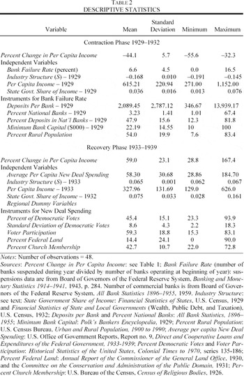
We estimate separate regressions for the contraction and recovery phases of the Great Depression. For the contraction phase, we regress the percentage change in state per capita income on the level of state per capita income in 1929, the industry structure variable (S), four regional dummy variables based on U.S. Census regions, the bank failure rate, and the ratio of state government expenditures to state income in 1929.¹²

In addition, we test for both spatial dependence in state per capita income growth and spatial correlation in the error structure of the model.

We define the bank failure rate as the annual average rate of bank suspensions during 1929–1932. We use instrumental variables to control for the influence of state income growth on bank failure rates. Our instruments reflect aspects of banking market structure and regulation that have been used to explain interstate differences in bank failure rates during the 1920s and 1930s.¹³

These include a measure of average bank size in 1929 (Deposits per Bank, 1929), the number of national banks divided by the number of all commercial banks within a state (Percent National Banks, 1929), the percentage of a state's bank deposits held in national banks (Percent Deposits in National Banks, 1929), the minimum capital requirement imposed on state banks (Minimum Capital, 1929), and the percentage of the state population living in rural areas (Percent Rural Population).¹⁴

For the recovery years 1933–1939, we regress the percentage change in state per capita income on New Deal spending, industry structure (S—constructed using income data from 1933 and 1939), state per capita income in 1933, the ratio of state expenditures to state personal income in 1932, and four regional dummy variables.¹⁵

We also consider spatial dependence and spatial error correlation.

Our New Deal spending variable is the average annual level of per capita New Deal spending (loans plus grants) over the period 1933–1939. We use instrumental variables to control for the possibility that New Deal spending was to some extent influenced by state income growth. Our instruments for New Deal expenditures are similar to those used by Robert Fleck and by Fishback, et al.: Average of the Democratic vote share in each presidential election from 1896 to 1932 (Percent of Democratic Votes); Standard deviation of the Democratic vote share from 1896 to 1932 (Standard Deviation of Democratic Votes); Average voter participation in each presidential election from 1896 to 1932 (Voter Participation); Federal land as a percent of a state's total land area in 1930 (Percent Federal Land); Percent of a state's population that belonged to a church in 1926 (Percent Church Membership).¹⁶

We estimate the following model separately for the contraction phase and recovery phase of the Great Depression:

where y is the percentage change in per capita personal income and X is the matrix of independent variables listed in Table 2 (state subscripts are suppressed). The scalar ρ provides an estimate of spatial dependence under the hypothesis that a change in per capita income in state i is correlated with changes in per capita income in neighboring states. The (N×N) spatial weights matrix, W, captures the effect of a change in per capita income in state i that results from a change in per capita income in bordering state l. Specifically, we define the elements of our weights matrix W = w*_il} as w*_il = w_il/[sum ]_lw_il where w_il = 1 if observations i and l (i ≠ l) share a common border and w_il = 0 otherwise. Because the spatially lagged dependent variable is endogenous by construction, we follow the literature and use spatially lagged independent variables (WX) as instruments for the spatially lagged dependent variable.

¹⁷

We also model and test for spatial error correlation in equation 2.

¹⁸

The first-order spatial autoregressive error structure can be expressed as follows:

where ε is the (N×1) vector of error terms, ϒ is a (N×1) component of the error terms made up of i.i.d. random variables, W is the (N×N) weights matrix with elements W = w*_il defined earlier, and λ is a scalar interpreted as the unobserved spatial error correlation coefficient. We estimate the models using generalized two-stage least squares (2SLS) where the spatial error coefficient (λ) is estimated by the generalized method of moments (GMM). The generalized 2SLS procedure produces consistent estimates of the model's parameters.

Our estimation procedure has several steps and is based on the methodology proposed by Harry Kelejian and Ingmar Prucha.

¹⁹

First, we obtain fitted values for all endogenous variables in the system by regressing each endogenous variable on the full set of independent variables and instruments for their respective era. The instrumented variables are the bank failure rate and Wy for the period 1929–1932, and New Deal spending and Wy for the period 1933–1939. We use the fitted values for these instrumented variables in equation 2, which we then estimate by OLS. For the specifications in which we consider a spatial error lag, we obtain the 2SLS residuals and calculate

using a GMM estimator. We then pre-multiply equation 2 by(I -

λW) and estimate this transformed equation using 2SLS.

EMPIRICAL RESULTS

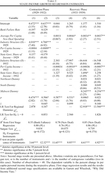
Regression results for the contraction (1929–1932) and recovery periods (1933–1939) are reported in Table 3. In addition to the second-stage coefficient estimates, we report the R² statistics from the first stage regressions for the bank failure rate, New Deal spending, and Wy (the spatially lagged dependent variable). To provide evidence on the validity of our instruments, we also report, first, a Sargan test statistic on the null hypothesis that the instruments are uncorrelated with the errors of the second stage regressions and, second, an F-test on the null hypothesis that the instruments in the first stage regressions are jointly different than zero. The Sargan test statistics indicate that we cannot reject the hypothesis that the instruments are uncorrelated with the second stage error terms and the F-tests reveal that the instruments are jointly different than zero.²⁰

We report two specifications for the contraction phase. Neither specification includes regional dummy variables, which we found to neither add explanatory power (based on likelihood ratio tests) nor influence the size and significance of the other coefficient estimates. Model 1 includes a spatial lag (with coefficient estimate ρ) and Model 2 includes both a spatial lag and a spatial error term (with coefficient estimate λ). The coefficient ρ is statistically significant in both specifications, and indicates that a 1 percentage point decline in the average per capita income growth rate of neighboring (border) states caused a state's per capita income growth rate to decline by about 0.5 percentage points.

We also find evidence that differences in the performance of major economic sectors contributed significantly to variation in state per capita income growth, as evidenced by the statistically significant coefficient on industry structure (S). States that derived a high percentage of personal income from sectors that performed especially poorly during 1929–1932, such as construction, farming, and mining, had significantly larger declines in per capita income than did more diversified states. States that were concentrated in sectors that performed relatively less poorly, such as services, finance, and transportation, experienced even smaller income declines.

Our results indicate that industry structure and spatial dependence can account for divergence in the level of state per capita incomes during 1929–1932. When these two variables are included in the model, the coefficient on the 1929 level of per capita income is negative (and statistically significant in model 2). Hence, within our model, industry structure and spatial dependence can fully explain the positive correlation between state per capita income in 1929 and income growth during 1929–1932. By contrast, we find no evidence that differences in bank failure rates or state government expenditures explain variation in state per capita income growth during 1929–1932.²¹

In addition, we find no evidence of spatial error correlation, as evidenced by the likelihood ratio (LR) test statistic presented in Table 3.

We report the estimates of four specifications for the recovery phase, 1933–1939. Models 5 and 6 include regional dummy variables, whereas models 3 and 4 do not. In contrast to the results for 1929–1932, we find that the regional dummy variables contribute (jointly) significant explanatory power to the regressions for 1933–1939. All else equal, the average Midwestern state had a 25 percentage point larger increase in nominal per capita income during this period than did the average Western state (the omitted group). The average increase across all states during the period was 59 percent (see Table 1). Further, a comparison of models 5 and 6 with models 3 and 4 reveals that spatial dependence in per capita income growth is not statistically significant when regional dummy variables are included in the model. This suggests that the degree of spatial dependence is different across regions, but that within each region there is no significant spatial dependence once unobserved regional variation in income growth is considered in the model. Finally, although we are unable to reject the hypothesis of no spatial correlation in the model error terms, a comparison of models 3 and 4 with models 5 and 6 reveals that, when we allow for spatial error correlation, the coefficients on the level of per capita income in 1933 are statistically significant. Their negative sign indicates that, all else equal, the higher a state's per capita income in 1933, the lower its per capita income growth rate during 1933–1939.

In contrast to the contraction phase of the Great Depression, we find no evidence that differences in income growth across major sectors contributed to variation in state per capita income growth during the recovery, as evidenced by the insignificant coefficients on industry structure. Compared with 1929–1932, income growth varied little across sectors during 1933–1939. Hence, differences in industry structure across states contributed little to variation in state per capita income growth rates.

Finally, we find evidence that New Deal spending patterns contributed to variation in state per capita income growth rates. The higher the level of federal expenditures and loans within a state, all else equal, the higher the state's per capita income growth rate.²²

Using the average of the New Deal spending coefficient estimates from models 5 and 6, we estimate that a $1 increase in New Deal spending per capita within a state would result in a 0.355 percentage point increase in per capita income growth. Or, a $27.19 (one standard deviation) increase in New Deal spending within a state would result in a 9.7 percentage point increase in per capita income growth.²³ Hence, our results are consistent with other recent studies in finding that New Deal spending patterns contributed significantly to variation in local economic performance.