4.1. Inviscid-limit flow states

In the case of inviscid flows, ${\it\gamma}_{{\it\nu}}=0$ , equation (4.1) has a trivial solution, $A_{s}(X)=0$ , for all ${\it\omega}$ , which represents the columnar states of an $x$ -independent swirling flow all along the pipe. Along this branch of steady states, there exist a series of critical states at specific swirl levels given by ${\it\omega}_{n}={\it\omega}_{B}+(2n-1)^{2}{\rm\pi}^{2}/(8{\it\beta}{\it\omega}_{B}L^{2})$ ( $n$ is a positive integer), where additional non-trivial steady-state solutions of (4.1) bifurcate. From a dynamical perspective, these states have a neutral mode of the dynamical problem (3.3) and (3.6). Solving the nonlinear problem (4.1), we find the series of branches of non-columnar states that appear in sequence as ${\it\omega}$ is increased above ${\it\omega}_{B}$ and bifurcate at ${\it\omega}_{n}$ . 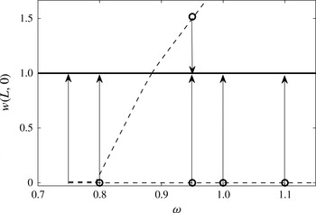Results of computations for the Lamb–Oseen vortex with $b=4$ are shown in figure 1. In this figure, the horizontal axis is the inlet swirl level ${\it\omega}$ in the range between 0.7 and 1.15. The vertical axis is a representative parameter of each solution given by $w_{c}=1+{\it\epsilon}_{1}C(A_{s})$ , where $C(A_{s})$ equals the first maximum value of $A_{s}(X)$ when the inlet slope is positive or the first minimum value of $A_{s}(X)$ when the inlet slope is negative.

Figure 1.

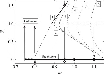
Bifurcation diagram of steady states for inviscid axisymmetric flow, Lamb–Oseen vortex, $b=4$ . Solid lines represent stable states and dashed lines represent unstable states. Numbers in boxes represent branch numbers. Arrows represent flow evolution at certain swirls. Circles represent the time-asymptotic results of simulations.

The branch of columnar states is represented by the line $w_{c}=1$ . Branch 1 bifurcates at the state with the first critical swirl, ${\it\omega}_{1}=0.8845$ , and exhibits a transcritical bifurcation. When ${\it\omega}<{\it\omega}_{1}$ , these states describe flow deceleration along the pipe centreline and acceleration near the wall, with minimum axial velocity at the outlet centreline that decreases as ${\it\omega}$ decreases from ${\it\omega}_{1}$ . When ${\it\omega}>{\it\omega}_{1}$ , these states describe acceleration along the pipe centreline and deceleration near the wall, with maximum axial velocity at the outlet centreline that increases as ${\it\omega}$ increases above ${\it\omega}_{1}$ . Branches 2, 3 and so on bifurcate at ${\it\omega}_{2}=0.8977,{\it\omega}_{3}=0.9241$ and so on, and describe steady waves with increasing wavenumber as branch number $n$ increases. These branches exhibit fold points at swirl levels ${\it\omega}_{2f}=0.8973,{\it\omega}_{3f}=0.9238$ and so on. 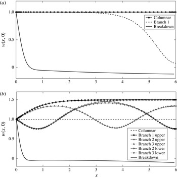Although some of the solutions have similar values of $w_{c}$ , they represent different solutions according to branch number and therefore have different shapes. Figure 2(a) shows an example of the centreline axial velocity, $w(x,0)$ , computed from the two possible equilibria found from the weakly nonlinear problem at ${\it\omega}=0.8$ , which is below ${\it\omega}_{1}$ . One solution is the trivial columnar solution and the other is a solitary-wave solution on branch 1 (the third solution shown in figure 2(a) is discussed in the next paragraph). Figure 2(b) shows another example of $w(x,0)$ computed from the six possible equilibria of the columnar flow branch and branches 1, 2 and 3 found from the weakly nonlinear problem at ${\it\omega}=0.95$ (the seventh solution shown in figure 2(b) is also discussed in the next paragraph). In a similar way, solutions are found for other swirl ratios in the range studied.

Figure 2.

The possible equilibria of a swirling flow at (a) three states at ${\it\omega}=0.8$ , and (b) seven states at ${\it\omega}=0.95$ .

In addition to the steady states found from the weakly nonlinear model (3.3), Wang & Rusak (Reference Wang and Rusak1997a ) proved that, for each ${\it\omega}$ in the range $0\leqslant {\it\omega}<{\it\omega}_{0}$ , there exists only one steady-state solution of the problem (2.1), which is the columnar flow solution. This additional critical swirl, ${\it\omega}_{0}$ , is less than ${\it\omega}_{1}$ and slightly changes with $L$ . For the Lamb–Oseen vortex with $b=4$ , it was found that ${\it\omega}_{0}=0.731$ in a very long pipe. The present simulations show that ${\it\omega}_{0}=0.738$ for the case of $L=6$ . A branch of breakdown states bifurcates at ${\it\omega}_{0}$ for which $w_{c}=0$ for all ${\it\omega}$ greater than ${\it\omega}_{0}$ ; see again figure 1. Wang & Rusak (Reference Wang and Rusak1997a ) also proved that the part of branch 1 with ${\it\omega}<{\it\omega}_{1}$ connects with the branch of breakdown states at ${\it\omega}_{0}$ , making the special breakdown state at ${\it\omega}_{0}$ a critical fold point. As a result, the inviscid steady-state version of problem (2.1) with assumed boundary conditions has three solutions in the range ${\it\omega}_{0}<{\it\omega}<{\it\omega}_{1}$ : the columnar solution, the decelerated flow state of branch 1 and the breakdown state. In the range ${\it\omega}_{1}<{\it\omega}<{\it\omega}_{2f}$ , there also exist three solutions: the columnar solution, the accelerated flow state of branch 1 and the breakdown state. When ${\it\omega}_{2f}<{\it\omega}<{\it\omega}_{3f}$ , there exist five solutions: the columnar state, the accelerated flow state of branch 1, two wavy states of branch 2 and the breakdown state. Additional steady-state solutions appear in sequence as ${\it\omega}$ is further increased, and they all include the columnar state, the accelerated flow state of branch 1 and the breakdown state among the numerous solutions. Figure 2(a,b) shows examples of the solution of the centreline axial velocity, $w(x,0)$ , for the computed breakdown states from the time-asymptotic state of the flow simulation at ${\it\omega}=0.8$ and $0.95$ , respectively, in addition to the other solutions found from the weakly nonlinear problem. Figures 1 and 2 demonstrate the complicated manifold of equilibria that the swirling flow in the pipe may take with the increase of inlet swirl from 0 to above ${\it\omega}_{1}$ .

Following Xu’s (Reference Xu2012) linear stability analysis of the various bifurcating states, that is based on (3.3), it can be shown that the columnar state has only asymptotically stable decaying in time modes when $0<{\it\omega}<{\it\omega}_{1}$ . However, the columnar states become unstable when ${\it\omega}>{\it\omega}_{1}$ , with instability modes that appear in sequence as ${\it\omega}$ increases. The states along branch 1 with ${\it\omega}_{0}<{\it\omega}<{\it\omega}_{1}$ are unstable, while the states along branch 1 with ${\it\omega}>{\it\omega}_{1}$ also have only asymptotically stable decaying in time modes. All states along branches 2, 3 and so on are unstable. The numerical computations described below show that the breakdown states bifurcating at ${\it\omega}_{0}$ are stable in the range of swirl studied. Therefore the dynamical problem (2.1) with assumed boundary conditions has only one stable steady-state solution when $0<{\it\omega}<{\it\omega}_{0}$ , which is the columnar state. When ${\it\omega}_{0}<{\it\omega}<{\it\omega}_{1}$ , there exist two possible stable steady states: the columnar state and the breakdown state. Initial conditions will dictate the flow evolution to one of these states. Sufficiently small disturbances on the columnar state will decay in time, while larger disturbances may evolve to breakdown states. When ${\it\omega}>{\it\omega}_{1}$ , there also exist two possible stable steady states: the accelerated flow state along branch 1 and the breakdown state. Again, initial conditions will dictate the flow dynamics. Computations using the unsteady weakly nonlinear problem as well as flow simulations show that, starting from small perturbations, the flow is more naturally drawn to the breakdown state; only specific large accelerating perturbations can lead the flow to the accelerated flow states. Figure 1 summarizes the expected dynamics of inviscid axisymmetric swirling flows in a finite-length pipe; solid lines represent stable states and dashed lines represent unstable states.

4.2. Simulations of inviscid flow evolution

We use the inviscid flow simulation code based on (2.1) and assumed boundary conditions to demonstrate the axisymmetric swirling flow dynamics. In all simulations, we assume an initial condition given by

(4.2) $$\begin{eqnarray}\left.\begin{array}{@{}rcl@{}}\displaystyle {\it\psi}(x,y,0)\ & =\ & \displaystyle {\it\psi}_{0}(y)+{\it\delta}{\it\epsilon}_{1}{\it\phi}_{B}(y)\sin \left(\frac{{\rm\pi}x}{2L}\right),\\ \displaystyle {\it\chi}(x,y,0)\ & =\ & \displaystyle -{\it\psi}_{0yy}-{\it\delta}{\it\epsilon}_{1}\left({\it\phi}_{Byy}-\frac{{\rm\pi}^{2}}{4L^{2}}{\it\phi}_{B}\right)\sin \left(\frac{{\rm\pi}x}{2L}\right),\\ \displaystyle K(x,y,0)\ & =\ & \displaystyle {\it\omega}K_{0}(y)+{\it\delta}{\it\epsilon}_{1}{\it\omega}_{B}\frac{K_{0y}}{{\it\psi}_{0y}}\sin \left(\frac{{\rm\pi}x}{2L}\right).\end{array}\right\}\end{eqnarray}$$

Here ${\it\delta}$ represents the initial perturbation size. When ${\it\delta}>0$ , the initial perturbation describes an accelerating flow along the pipe centreline; while when ${\it\delta}<0$ , it describes a decelerating flow. Results of simulations are presented as well as compared to the weakly nonlinear predictions.

The inviscid flow simulations show that, starting with either small or large, decelerating or accelerating flow perturbations, the flow always evolves to a columnar state when $0\leqslant {\it\omega}<{\it\omega}_{0}$ , as predicted by the theory described above. In the range of incoming swirl ${\it\omega}_{0}\leqslant {\it\omega}\leqslant {\it\omega}_{1}$ , sufficiently small perturbations evolve to the columnar state. However, larger perturbations evolve to breakdown states. For example, the simulations show that, starting from initial flow perturbation with ${\it\delta}>-12$ at ${\it\omega}=0.8$ , the flow always evolves to a columnar state. On the other hand, a larger initial perturbation with ${\it\delta}<-12$ always evolves to the breakdown state at ${\it\omega}=0.8$ .

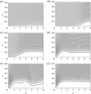
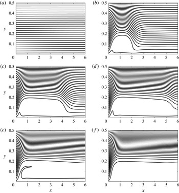
Figure 3 describes a representative example of the evolution of an initially perturbed columnar flow with ${\it\delta}=-15$ to the breakdown state at ${\it\omega}=0.8$ . In each panel, flow runs from left to right, the left edge of the panel is the inlet, the right edge is the outlet, the bottom edge is the centreline ${\it\psi}=0$ and the upper edge is the pipe wall ${\it\psi}=0.5$ . There are 25 equispaced contour lines in each panel, ranging from 0.01 to 0.49. At this below-critical inlet swirl case, the initial perturbation (figure 3 a) grows near the outlet to a finite-size near-stagnation zone at $t=66$ (figure 3 b) that moves upstream towards the inlet (figure 3 c,d). Once near the inlet, waves are generated along the interface of the zone and are convected downstream (figure 3 e) until a time-asymptotic state with a breakdown zone that stretches to the outlet is established when $t>153$ (figure 3 f). Over most of the domain ( $x>2$ ) the flow is parallel to the finite-size breakdown zone. This flow evolution is described schematically in figure 1 by the arrow at ${\it\omega}=0.8$ pointing from a nearly columnar flow where $w_{c}=0.1$ to the breakdown state at that swirl level for which $w_{c}=-0.11$ .

Figure 3.

Streamfunction contour-line snapshots of flow evolution from a near-columnar state to a breakdown state when ${\it\omega}=0.8$ at (a) $t=0$ , (b) $t=66$ , (c) $t=105$ , (d)  $t=124$ , (e)  $t=134$ and ( f)  $t=153$ . Initial perturbation is with ${\it\delta}=-15$ .

Similar results are found from simulations at various ${\it\omega}$ between ${\it\omega}_{0}$ and ${\it\omega}_{1}$ . Smaller limit perturbations are needed to access the breakdown states as ${\it\omega}$ approaches ${\it\omega}_{1}$ . Moreover, by starting from the breakdown state at ${\it\omega}=0.75$ and reducing ${\it\omega}$ in small steps to 0.738, we find that the flow returns to a columnar state (details are not shown). This process is presented in figure 1 by the arrow at ${\it\omega}=0.738$ that starts at $w_{c}=0$ and ends at $w_{c}=1$ . This computation demonstrates that ${\it\omega}_{0}=0.738$ for a swirling flow in a pipe with length $L=6$ . Also, a hysteresis loop in the cross-over between the columnar and breakdown states is realized in the range of ${\it\omega}_{0}$ to ${\it\omega}_{1}$ .

Figure 4 presents for ${\it\omega}=0.95>{\it\omega}_{1}$ streamfunction contour line snapshots of the flow evolution from an initially perturbed near-columnar flow state with ${\it\delta}=-4$ to a breakdown state. The small initial perturbation (figure 4 a) focuses near the inlet, grows in time and changes in space, forming an increasing flow deceleration along the centreline. At $t=60$ , the disturbance is sufficiently large to form a stagnation point along the centreline near the inlet (figure 4 b). From this stage, a low-speed zone around the centreline is established and spreads in time both radially and axially (figure 4 c–e). Eventually, when $t>196$ , the flow stabilizes on a time-asymptotic breakdown state, which describes a swirling flow that splits around a finite-size, nearly stagnant zone that stretches from near the inlet to the outlet (figure 4 f). Over most of the domain ( $x>2$ ) the flow is parallel to the finite-size breakdown zone. This flow evolution is described schematically in figure 1 by the arrow at ${\it\omega}=0.95$ pointing from a nearly columnar flow where $w_{c}=0.89$ to the breakdown state at that swirl level for which $w_{c}=-0.05$ .

Figure 4.

Streamfunction contour-line snapshots of flow evolution from a near-columnar state to a breakdown state when ${\it\omega}=0.95$ at (a) $t=0$ , (b) $t=60$ , (c) $t=85$ , (d)  $t=110$ , (e)  $t=159$ and ( f) $t=196$ . Initial perturbation is with ${\it\delta}=-4$ .

Figure 5 presents another example of flow dynamics to breakdown at a higher incoming swirl ratio, ${\it\omega}=1.1$ . The figure shows the flow evolution from an initially perturbed near-columnar flow state with ${\it\delta}=-4$ (figure 5 a) to a breakdown state at this swirl level (figure 5 f). This flow evolution is described schematically in figure 1 by the arrow at ${\it\omega}=1.1$ pointing from $w_{c}=0.89$ to $w_{c}=0$ .

Figure 5.

Streamfunction contour-line snapshots of flow evolution from a near-columnar state to a breakdown state when ${\it\omega}=1.1$ at (a) $t=0$ , (b) $t=36$ , (c) $t=58$ , (d)  $t=68$ , (e)  $t=80$ and ( f) $t=102$ . Initial perturbation is with ${\it\delta}=-4$ .

Results from inviscid flow simulations for the whole range of ${\it\omega}$ between ${\it\omega}_{1}=0.8845$ and 1.15 show similar evolution of initially small decelerating flow perturbations on the columnar flow to breakdown states. We note the differences between the development of the breakdown zone at the below-critical swirl case and the above-critical swirl case (compare figures 3–5). At below-critical swirls, the breakdown waves build up near the outlet and propagate upstream, while at above-critical swirls, waves focus near the inlet and the breakdown zone spreads downstream.

When ${\it\omega}_{1}<{\it\omega}<{\it\omega}_{2}$ , accelerating flow perturbations evolve to the accelerated flow state on branch 1; see examples in Rusak et al. (Reference Rusak, Wang, Xu and Taylor2012). However, when ${\it\omega}>{\it\omega}_{2}$ , initially small accelerating flow perturbations are first attracted to the upper states of branch 2 but then turn and evolve to breakdown states. Only relatively large accelerating initial flow perturbations allow an access to the stable states along the part of branch 1 with ${\it\omega}>{\it\omega}_{2}$ . For example, when ${\it\omega}=0.95$ and ${\it\delta}<21$ , the flow evolves to the breakdown state; while a large perturbation with ${\it\delta}>21$ leads the flow to settle on the accelerated flow state (details not shown). Starting from ${\it\delta}=24$ at ${\it\omega}=0.95$ , the flow evolves to the accelerated flow state on branch 1. This process is demonstrated in figure 1 by the arrow at ${\it\omega}=0.95$ that starts at $w_{c}=1.6$ and ends at $w_{c}=1.51$ . Higher values of ${\it\delta}$ are needed to settle on these flow states at higher ${\it\omega}$ .

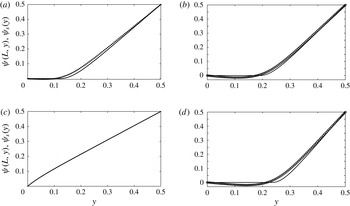
To demonstrate the correlation between the time-asymptotic states shown in figures 3–5 and the predicted states according to Wang & Rusak (Reference Wang and Rusak1997a ), we present for each state a cross-section of the outlet streamfunction profile, ${\it\psi}(L,y)$ (see figure 6). Also shown for each swirl level are the corresponding solutions of the columnar Squire–Long equation for the Lamb–Oseen vortex with $b=4$ as predicted by the theory of Wang & Rusak (Reference Wang and Rusak1997a ). It can be seen that the two solutions agree nicely for the breakdown state at ${\it\omega}=0.8$ and for the accelerated flow state at ${\it\omega}=0.95$ (figure 6 a,c). The two solutions at ${\it\omega}=0.95$ and ${\it\omega}=1.1$ are similar (figure 6 b,d). The small differences between these solutions result from the fact that in the simulations $L=6$ , which is not sufficiently long for the computation to fully match the theoretical prediction, which assumes a much longer pipe. Therefore, the simulation time-asymptotic states describe a slightly smaller breakdown zone than predicted by the theory. We also emphasize that, as the flow in figures 3–5 evolves to a steady state, the separation zone becomes naturally a near-stagnation zone, in accordance with Batchelor’s (Reference Batchelor1956) condition for steady inviscid-limit flows with a separation zone.

Figure 6.

A comparison between the time-asymptotic outlet streamfunction profile ${\it\psi}(L,y)$ of the flow states (dotted line/circles) and the predicted outlet state ${\it\psi}_{s}(y)$ for a very long pipe according to the theory of Wang & Rusak (Reference Wang and Rusak1997a ) (solid line): (a)  ${\it\omega}=0.8$ (breakdown state), (b)  ${\it\omega}=0.95$ (breakdown state), (c)  ${\it\omega}=0.95$ (accelerated flow state) and (d)  ${\it\omega}=1.1$ (breakdown state).

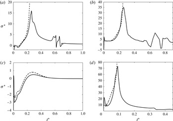
In addition, figure 7 shows the computed rescaled growth rate, ${\it\sigma}^{\ast }={\it\sigma}/{\it\epsilon}_{1}^{3/2}$ , of the perturbation as a function of rescaled time, $t^{\ast }={\it\epsilon}_{1}^{3/2}t$ , for each of the cases discussed above from the simulation and from the weakly nonlinear model, where ${\it\epsilon}_{1}=1/L^{2}$ . We note that these rescaled variables result from the weakly nonlinear approach in § 3 and that the use of the variable $t^{\ast }$ provides a rescaling of time such that phenomena occur over $t^{\ast }\sim O(1)$ time scale (here, $L=6$ and ${\it\epsilon}_{1}=1/36$ ). Good agreement is found in the whole range of swirl between the two predictions as long as the perturbation grows from a small disturbance to the state where a stagnation point appears for the first time. We note that the initial perturbation contains various higher-order modes that are stable. The oscillations at the beginning $(0<t^{\ast }<0.05)$ are related to the decay of the initial perturbation to the dominant linear mode. Such a decay process may look quite oscillatory since the various higher-order modes decay at different rates. We also note that the initial stage of the process of breakdown involves faster-than-exponential growth of perturbations, and this process must be taken into account in any nonlinear control approach of the breakdown process.

Figure 7.

A comparison between the evolution of the perturbation rescaled growth rate according to the weakly nonlinear model (dashed line) and the simulation (solid line) at (a)  ${\it\omega}=0.8$ , ${\it\delta}=-15$ , (b)  ${\it\omega}=0.95$ , ${\it\delta}=-4$ , (c)  ${\it\omega}=0.95$ , ${\it\delta}=-24$ and (d)  ${\it\omega}=1.1$ , ${\it\delta}=-4$ .

Also, the simulations show that the growth rate reaches a maximum at the state where a stagnation point appears and then it decreases as the breakdown zone evolves to the time-asymptotic state. This process of breakdown involves structural changes of the flow in the radial direction. On the other hand, the weakly nonlinear theory exhibits a singular growth of the perturbation after a stagnation point appears in the flow. This results from the limitation of the weakly nonlinear approach, which involves a fixed-in-time profile of the perturbation in the radial direction.

4.3. High- $\mathit{Re}$ flow states

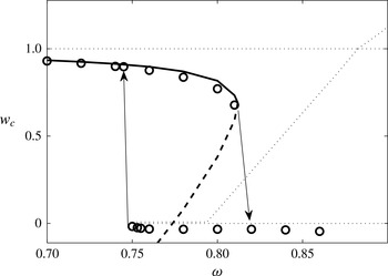
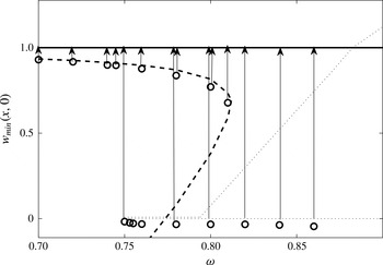
In the case of viscous flows, ${\it\gamma}_{{\it\nu}}>0$ , and problem (4.1) has no trivial solution. Numerical solutions of (4.1) are computed at $\mathit{Re}=4000$ for a pipe length $L=6$ , in the range of incoming swirl $0.7\leqslant {\it\omega}\leqslant 0.8845$ . Figure 8 presents the computed $w_{c}$ of these states as a function of swirl level. Here the solid line followed by the folding dashed line is from the weakly nonlinear problem. Also shown for reference is the bifurcation diagram for the inviscid flow case (dotted lines). In the high- $\mathit{Re}$ flow case, the branch of inviscid columnar states for $0<{\it\omega}<{\it\omega}_{1}$ and the branch 1 of inviscid solutions in the swirl range ${\it\omega}_{0}<{\it\omega}<{\it\omega}_{1}$ combine together to form a branch of steady states with a fold point at a swirl level denoted by ${\it\omega}_{1{\it\nu}}$ . For example, when $\mathit{Re}=4000$ and $L=6$ , we find that ${\it\omega}_{1{\it\nu}}=0.812$ . The upper part of this branch of solutions ( $0<{\it\omega}<{\it\omega}_{1{\it\nu}}$ ) describes (solid line in figure 8) nearly columnar flows decelerating along the centreline and accelerating along the pipe wall. Flow disturbances from columnar are relatively small and the flow achieves minimum speed at the outlet centreline, i.e.  $w_{c}=w(L,0)$ . The lower part of the branch of solutions that folds back ( ${\it\omega}<{\it\omega}_{1{\it\nu}}$ ) describes (dashed line in figure 8) solitary-wave states with large deceleration along the centreline, specifically focused near the outlet.

Figure 8.

Bifurcation diagram of steady states for $\mathit{Re}=4000$ , axisymmetric flow, Lamb–Oseen vortex, $b=4$ . Lines represent solutions of weakly nonlinear theory; solid lines are stable solutions and dashed lines are unstable solutions. Circles represent results from present simulations. Arrows represent flow evolution at certain swirls. Dotted lines represent the inviscid flow bifurcation diagram for reference.

This special fold behaviour of viscous swirling flows as described by the weakly nonlinear approximation is similar to the computations of Beran & Culick (Reference Beran and Culick1992) for a pipe with non-dimensional length $L=15$ and with no contraction. The numerical steady flow computations of Beran & Culick (Reference Beran and Culick1992) also show the appearance of steady breakdown states in a Lamb–Oseen vortex with $b=4$ when ${\it\omega}$ is greater than another special swirl level denoted by ${\it\omega}_{0{\it\nu}}$ , where ${\it\omega}_{0{\it\nu}}<{\it\omega}_{1{\it\nu}}$ . These breakdown states are characterized by a swirling flow splitting around a closed separation zone. In addition, the simulations show the existence of a continuous branch of solitary-wave states connecting between ${\it\omega}_{1{\it\nu}}$ and ${\it\omega}_{0{\it\nu}}$ . Furthermore, the unsteady flow simulations of Beran (Reference Beran1994) and Lopez (Reference Lopez1994) show that the non-columnar states and the breakdown states are stable while the solitary-wave states are unstable and are not found as time-asymptotic solutions. Similarly, our linear stability analysis of the various steady states found from the solution of (4.1) show that the non-columnar states are asymptotically stable while the solitary-wave states are unstable (see Xu Reference Xu2012). Therefore, from a dynamical perspective, only one near-columnar stable state exists when ${\it\omega}<{\it\omega}_{0{\it\nu}}$ , two possible stable states exist when ${\it\omega}_{0{\it\nu}}<{\it\omega}<{\it\omega}_{1{\it\nu}}$ (a near-columnar state and a breakdown state) and only one stable breakdown state exists in a range of swirl above ${\it\omega}_{1{\it\nu}}$ .

4.4. Simulations of high- $\mathit{Re}$ flow evolution

The present unsteady viscous flow simulations for the Lamb–Oseen vortex with $b=4$ in a pipe with $L=6$ , shown by open circles in figure 8, support the flow dynamics described above. Results show the successive appearance of steady, near-columnar states with increased flow deceleration along the pipe when ${\it\omega}$ is increased in the range $0.7\leqslant {\it\omega}\leqslant 0.81$ (circles with $w_{c}>0$ in figure 8). Here, $w_{c}=w(L,0)$ . When ${\it\omega}$ is further increased from 0.81 to 0.82, the flow evolves from the initial near-columnar state at 0.81 to a breakdown state at 0.82. This is represented by the arrow in figure 8 connecting the point ( ${\it\omega}=0.81,w_{c}=0.69$ ) and the point ( ${\it\omega}=0.82,w_{c}=-0.03$ ). 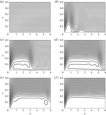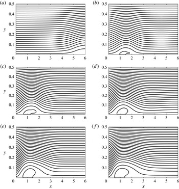The details of this flow transition to a breakdown state are shown in figure 9. There are 26 equispaced contour lines in each panel, ranging from 0 to 0.49. The initial wave grows near the outlet (figure 9 a), travels upstream (figure 9 b), grows in radial size around $x=1$ (figure 9 c) and establishes a compact separation (breakdown) zone that fluctuates at its back side between $x=1$ and $x=2$ at a low frequency (figure 9 d–f). This transition also demonstrates that the branch of near-columnar states folds at ${\it\omega}_{1{\it\nu}}=0.812$ .

Figure 9.

Streamfunction contour-line snapshots of flow evolution at $\mathit{Re}=4000$ from an initial near-columnar state at ${\it\omega}=0.81$ to the breakdown state at ${\it\omega}=0.82$ at (a)  $t=0$ , (b)  $t=100$ , (c) $t=200$ , (d) $t=300$ , (e) $t=340$ and ( f)  $t=380$ .

Starting from the breakdown state at ${\it\omega}=0.82$ , the present viscous flow simulations are successively continued in small steps to both higher swirl ratios up to ${\it\omega}=0.86$ and to lower swirl ratios down to ${\it\omega}=0.75$ . These states are represented by the circles with $w_{c}<0$ in figure 8. A snapshot of each of the various fluctuating breakdown states in this range of swirl is shown in figure 10. It can be seen that, as ${\it\omega}$ is increased from 0.75, the breakdown zone moves upstream and increases in radial extent. 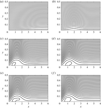Note that at $\mathit{Re}=4000$ the breakdown zones are compact with axial extent of about one pipe radius and the swirling flow wraps around them and is significantly slowed down in the range downstream of the zone. 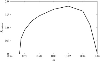These breakdown states are different from the inviscid long and wide breakdown states shown in figures 3–5, which may characterize much higher- $\mathit{Re}$ flows. The non-dimensional dominant fluctuation frequencies at the back of the breakdown zones as a function of ${\it\omega}$ are summarized in figure 11. The frequency is nearly zero at ${\it\omega}=0.75$ and 0.86 and achieves a maximum value of 1.8 at ${\it\omega}=0.82$ .

Figure 10.

Streamfunction contour-line snapshots of breakdown states at $\mathit{Re}=4000$ at (a)  ${\it\omega}=0.75$ , (b) ${\it\omega}=0.76$ , (c) ${\it\omega}=0.78$ , (d) ${\it\omega}=0.80$ , (e) ${\it\omega}=0.84$ and ( f)  ${\it\omega}=0.86$ .

Figure 11.

Non-dimensional frequency of oscillations of breakdown states as a function of ${\it\omega}$ , at $\mathit{Re}=4000$ .

Starting from the breakdown state at ${\it\omega}=0.75$ and reducing the swirl to 0.745, the flow evolves back to the near-columnar state at this swirl level (details not shown). This process demonstrates that ${\it\omega}_{0{\it\nu}}=0.748$ when $\mathit{Re}=4000$ and $L=6$ and is shown by the arrow in figure 8 pointing upwards from the point ( ${\it\omega}=0.748,w_{c}=-0.01$ ) to the point ( ${\it\omega}=0.745,w_{c}=0.91$ ).

The present simulations and weakly nonlinear computations show that, within the range of swirl ratios studies, at $\mathit{Re}=4000$ there is only one stable near-columnar state when $0<{\it\omega}<{\it\omega}_{0{\it\nu}}=0.748$ . There exist three states when ${\it\omega}_{0{\it\nu}}=0.748<{\it\omega}<{\it\omega}_{1{\it\nu}}=0.812$ : a stable near-columnar state, an unstable solitary-wave state and an oscillating breakdown state. Only a breakdown state with fluctuations at the back of the separation zone exists in the range of swirl ${\it\omega}_{1{\it\nu}}=0.812<{\it\omega}\leqslant 0.86$ , which is an attractor of flow dynamics at these swirl ratios. These results agree with those of Beran & Culick (Reference Beran and Culick1992), Beran (Reference Beran1994) and Lopez (Reference Lopez1994).

6.1. Control of inviscid-limit swirling flows

Figure 14 presents snapshots of the actively controlled dynamics of a Lamb–Oseen vortex with $b=4$ , ${\it\omega}=0.95>{\it\omega}_{1}$ and $L=6$ . In each panel, flow runs from left to right, the left edge is the inlet, the right edge is the outlet, the bottom edge is the centreline ${\it\psi}=0$ and the upper edge is the pipe wall $y=0.5$ . We continued the simulation shown in figure 4, and at time $t_{0}=196.6$ ( $t_{0}^{\ast }=0.91$ ), where the flow had established a breakdown state, we initiated a control command with gain ${\it\gamma}=2$ and rise time of $T_{s}=1.5$ ( $T_{s}^{\ast }=0.007$ ). Figure 15(a) shows the perturbation’s minimum, maximum and outlet values of the axial velocity after control has been initiated. Figure 15(b) shows the control command $U_{c}$ as a function of $t^{\ast }$ . Under the initial injection, the control command rises from zero to a maximum value of $U_{c}=0.115$ ( ${\dot{m}}_{in}=1.38$ , $C_{{\it\mu}}=0.159$ ) at $t=199$ ( $t^{\ast }=0.921$ ). The initial large breakdown zone (figure 14 a) collapses to a much smaller zone near the inlet over a short time period of two time units (figure 14 b at $t=199$ ). As a result, the radial velocity at the inlet decreases at $y_{m}=0.11$ and the injection is reduced. This is followed up by a further diffusion of the zone over time (figure 14 c,d) with further reduction of injection. At $t=217$ ( $t^{\ast }=1.005$ ), the wall injection turns into slight wall suction, which grows to a minimum of $U_{c}=-0.0025~({\dot{m}}_{in}=-0.03,C_{{\it\mu}}=0.000075)$ at $t=227$ ( $t^{\ast }=1.051$ ) and then decays to zero. The accelerated flow along the centreline decays exponentially over time (figure 14 e, f) and the flow stabilizes on a columnar state when $t>432$ ( $t^{\ast }>2$ ). The non-dimensional control response time is ${\rm\Delta}t\sim 236$ . This demonstrates for the first time the feasibility of eliminating the vortex breakdown state and stabilizing on a columnar state in an above-critical swirl flow based on the axisymmetric Euler equations. Figures 4 and 14 together show a complete continuous process of how a columnar vortex flow in a pipe with above-critical swirl evolves from a small perturbation to a breakdown state and then, with the initiation of active feedback flow control, returns to a columnar state with an asymptotically decaying control command.

Figure 15.

Actively controlled inviscid flow properties as a function of time when ${\it\omega}=0.95$ : (a) $w_{min},w_{max},w(L,0)$ and (b) $U_{c}$ . Control command is with ${\it\gamma}=2$ .

We further explore the capabilities to control swirling flows in a pipe at higher swirl levels. Successful control has been achieved for all swirl levels up to ${\it\omega}=1.15$ , which is 30 % above the critical value. The controlled flow dynamics of a Lamb–Oseen vortex with $b=4$ , ${\it\omega}=1.1>{\it\omega}_{1}$ and $L=6$ is shown in figures 16 and 17. We again continued the simulation shown in figure 5, and at time $t_{0}=102.2$ ( $t_{0}^{\ast }=0.474$ ), where the flow had established a time-asymptotic breakdown state, we initiated a control command with gain ${\it\gamma}=1.5$ and rise time of $T_{s}=7.5$ ( $T_{s}^{\ast }=0.035$ ). The dynamics as well as the control command are similar to those shown in figures 14 and 15, but occur over a shorter time scale. The control command increases from zero to a maximum injection of $U_{c}=0.24$ ( ${\dot{m}}_{in}=2.88$ , $C_{{\it\mu}}=0.691$ ), at $t=106$ ( $t^{\ast }=0.491$ ), then quickly decreases, turns into suction with a minimum of $U_{c}=-0.038$ ( ${\dot{m}}_{in}=-0.456$ , $C_{{\it\mu}}=0.017$ ) at $t=115$ ( $t^{\ast }=0.532$ ) and then decays to zero. The control command is higher than in the previous case to compensate for the stronger vortex breakdown with larger radial velocity at the inlet at the higher swirl. The flow returns to a columnar state when $t>300$ ( $t^{\ast }>1.4$ ). The non-dimensional control time response is ${\rm\Delta}t\sim 200$ . Again, figures 5 and 16 together show another example of a complete continuous process of how a columnar vortex flow in a pipe with above-critical swirl evolves from a small perturbation to a breakdown state and then, with the initiation of active flow control, returns to a columnar state with an asymptotically decaying control command.

Figure 16.

Streamfunction contour-line snapshots of actively controlled inviscid flow evolution from an initial vortex breakdown state to a columnar state when ${\it\omega}=1.1$ at (a)  $t=102.2$ , (b) $t=102.4$ , (c) $t=107.4$ , (d) $t=116.4$ , (e) $t=142$ and ( f)  $t=272$ . Control command is with ${\it\gamma}=1.5$ .

Figure 17.

Actively controlled inviscid flow properties as a function of time when ${\it\omega}=1.1$ : (a) $w_{min},w_{max},w(L,0)$ and (b) $U_{c}$ . Control command is with ${\it\gamma}=1.5$ .

We also demonstrate the ability of the proposed control law to eliminate accelerated flow states when ${\it\omega}>{\it\omega}_{1}$ . For example, in the case of ${\it\omega}=0.95$ and $L=6$ , we started from the time-asymptotic accelerated flow state, and at time $t_{0}=1253$ ( $t_{0}^{\ast }=5.8$ ) we initiated the active control command. Here the control gain is ${\it\gamma}=2$ and the rise time is $T_{s}=1.5$ . Figure 18(a) shows the maximum, minimum and outlet values of the axial velocity as a function of time ( $t^{\ast }$ ), and figure 18(b) shows the corresponding evolution of the control command, $U_{c}$ . In this case, suction is first introduced and causes the flow to decelerate with a minimum suction of $U_{c}=-0.0043$ ( ${\dot{m}}_{in}=-0.052$ , $C_{{\it\mu}}=0.0002$ ) at time $t=1268$ ( $t^{\ast }=5.87$ ). Then, the perturbation decays over time and the suction is reduced. The controller exhibits oscillatory decay, which involves changes between slight suction and injection, accompanied by an oscillatory decay of the minimum, maximum and outlet axial velocities to unity. The non-dimensional control time response is ${\rm\Delta}t\sim 300$ . Similar results are found for the elimination of all accelerated flow states in the range of ${\it\omega}_{1}\leqslant {\it\omega}\leqslant 1$ .

Figure 18.

Actively controlled inviscid flow properties as a function of time when ${\it\omega}=0.95$ from an initial accelerated flow state to a columnar state: (a) $w_{min},w_{max},w(L,0)$ and (b) $U_{c}$ . Control command is with ${\it\gamma}=2$ .

The control of the breakdown states in the range of ${\it\omega}_{0}\leqslant {\it\omega}\leqslant {\it\omega}_{1}$ has been investigated as well. Figure 19 shows the example of the controlled flow dynamics at ${\it\omega}=0.8$ and $L=6$ starting from the breakdown state at this swirl at $t_{0}=214$ ( $t_{0}^{\ast }=0.991$ ). A gain of ${\it\gamma}=-4$ ( ${\it\gamma}<0$ since ${\it\omega}<{\it\omega}_{1}$ ) and rise time of $T_{s}=1.5$ are used. The perturbation’s minimum, maximum and outlet values of the axial velocity are presented in figure 19(a) and the evolution of the control command is shown in figure 19(b). The initial injection that rises up to a maximum of $U_{c}=0.05$ ( ${\dot{m}}_{in}=0.6$ , $C_{{\it\mu}}=0.03$ ) at $t=219$ ( $t^{\ast }=1.015$ ) enforces a decay of the breakdown zone and flow acceleration along the centreline. The control command decreases to near zero at $t=259$ ( $t^{\ast }=1.2$ ). However, the flow continues to decay exponentially and approaches a columnar state when $t>346$ ( $t^{\ast }>1.6$ ) owing to the natural stability of the below-critical base flow. The non-dimensional control response time is ${\rm\Delta}t\sim 130$ . Similar control results of breakdown states have been achieved with proper control parameters for the range $0.75\leqslant {\it\omega}\leqslant 0.87$ . Figures 3 and 19 together show a complete continuous process of how a columnar vortex flow in a pipe with swirl level between ${\it\omega}_{0}<{\it\omega}<{\it\omega}_{1}$ evolves from a large perturbation to a breakdown state and then, with the initiation of active flow control, stabilizes on a columnar state with an asymptotically decaying control command.

Figure 19.

Actively controlled inviscid flow properties as a function of time when ${\it\omega}=0.8$ from an initial breakdown state to a columnar state: (a)  $w_{min}$ , $w_{max}$ , $w(L,0)$ and (b)  $U_{c}$ . Control command is with ${\it\gamma}=-4$ .

The inviscid flow simulations demonstrate that the proposed control approach with proper control parameters is able to completely eliminate the breakdown states in the range of swirl from ${\it\omega}_{0}$ to ${\it\omega}=1.15$ and to establish a stable controlled columnar state in this swirl range. Essentially, the closed loop controlled flow has a completely different bifurcation diagram than the natural flow (refer to figure 1). This idea is demonstrated in figure 20. The arrows represent the controlled dynamics of the flow from breakdown states to controlled columnar states with a wide basin of attraction. Using the active feedback control law, the envelope of operation of stable columnar states is increased up to at least 30 % above ${\it\omega}_{1}$ and 56 % above ${\it\omega}_{0}$ , while no stable breakdown and no stable accelerated flow states can exist in this range of swirl. Note, however, that the controller must remain active for all the time to maintain a stable columnar state.

Figure 20.

Diagram of states for inviscid axisymmetric flow when active flow control is applied, Lamb–Oseen vortex, $b=4$ . Dashed lines represent equilibrium natural states. Arrows represent controlled flow evolution at certain swirls from initial states (represented by the circles) to columnar states (represented by the solid lines).

Figure 21.

Actively controlled flow properties as a function of time for various ${\it\omega}$ at $\mathit{Re}=4000$ from an initial near-columnar state to an almost columnar state: (a)  $w_{min}$ , $w_{max}$ , $w(L,0)$ and (b)  $U_{c}$ for ${\it\omega}=0.7$ ; (c)  $w_{min}$ , $w_{max}$ , $w(L,0)$ and (d)  $U_{c}$ for ${\it\omega}=0.78$ ; and (e)  $w_{min}$ , $w_{max}$ , $w(L,0)$ and ( f)  $U_{c}$ for ${\it\omega}=0.81$ . Control command is with ${\it\gamma}=-2$ .

6.2. Control of high- $\mathit{Re}$ swirling flows

We demonstrate the control ideas on a Lamb–Oseen vortex flow with $b=4$ entering a pipe of length $L=6$ at $\mathit{Re}=4000$ . We first focus on the control of the near-columnar states at $0\leqslant {\it\omega}\leqslant {\it\omega}_{1{\it\nu}}$ . Figure 21 describes examples of the controlled flow dynamics at ${\it\omega}=0.7$ , 0.78 and 0.81, where the initial state in all cases is the steady near-columnar state. In all cases we use ${\it\gamma}=-2$ and $T_{s}=1.5$ . The decay of the perturbation and return of the controlled flow to an almost columnar state is evident from figure 21(a,c,e). The control injection command increases to a maximum and then stabilizes on the same constant value for all cases, $U_{c}=0.0017$ ( ${\dot{m}}_{in}=0.020$ , $C_{{\it\mu}}=0.00003$ ), which is associated with the passive part of the control law to eliminate the viscous effect (see figure 21 b,d, f). This time-asymptotic continuous injection forces a slight contraction on the flow, which together with swirl generates a slight change of the time-asymptotic state from columnar. The non-dimensional control response time is ${\rm\Delta}t\sim 50$ . Note that other values of ${\it\gamma}$ can be used, including ${\it\gamma}=0$ , to stabilize the flow to an almost columnar state, but the process may be slower. When ${\it\gamma}=0$ , only the passive part of the control command is applied and the flow stabilizes through the natural inviscid stability of the below-critical states.

We show now the flow control processes to eliminate the breakdown states in a pipe of length $L=6$ at $\mathit{Re}=4000$ in the range ${\it\omega}_{0{\it\nu}}\leqslant {\it\omega}\leqslant 0.87$ . Figures 22 and 23 provide the details of the controlled flow at ${\it\omega}=0.78$ . The initial state is the flow state at $t_{0}=1379$ ( $t^{\ast }=6.385$ ) shown in figure 10(c). The control parameters are ${\it\gamma}=-1$ and $T_{s}=1.5$ . The initial breakdown zone (figure 22 a) is diffused over time by the flow injection (figure 22 b,c), pushed out along the centreline (figure 22 d,e), and the flow returns to an almost columnar state (figure 22 f). The perturbation’s properties decay with some oscillation at the beginning and then exponentially decay to a value near unity (figure 23 a). The control injection command (figure 23 b) increases to a maximum value, $U_{c}=0.043$ ( ${\dot{m}}_{in}=0.516$ , $C_{{\it\mu}}=0.022$ ) at $t=1382$ ( $t^{\ast }=6.398$ ) and then decays to a constant value, 0.0017. The non-dimensional control response time is ${\rm\Delta}t\sim 120$ .

Figure 22.

Streamfunction contour-line snapshots of actively controlled flow evolution from an initial vortex breakdown state to an almost columnar state when ${\it\omega}=0.78$ and $\mathit{Re}=4000$ at (a)  $t=1379$ , (b) $t=1379.8$ , (c) $t=1388.8$ , (d) $t=1393.8$ , (e)  $t=1409.8$ and ( f)  $t=1495$ . Control commands are with ${\it\gamma}=-1$ .

Figure 23.

Actively controlled flow properties as a function of time for ${\it\omega}=0.78$ and $\mathit{Re}=4000$ from a breakdown state to an almost columnar state: (a)  $w_{min},w_{max},w(L,0)$ and (b) $U_{c}$ . Control command is with ${\it\gamma}=-1$ .

Figure 24.

Streamfunction contour-line snapshots of actively controlled flow evolution from an initial vortex breakdown state to an almost columnar state when ${\it\omega}=0.86$ and $\mathit{Re}=4000$ at (a)  $t=1280$ , (b) $t=1282$ , (c) $t=1284$ , (d) $t=1287$ , (e) $t=1297$ and ( f)  $t=1327$ . Control commands are with ${\it\gamma}=-4$ .

Figure 25.

Actively controlled flow properties as a function of time for ${\it\omega}=0.86$ at $\mathit{Re}=4000$ from an initial near-columnar state to an almost columnar state: (a)  $w_{min}$ , $w_{max}$ , $w(L,0)$ and (b)  $U_{c}$ . Control command is with ${\it\gamma}=-4$ .

Figure 26.

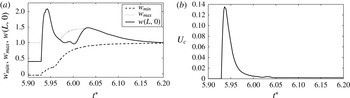
Diagram of states for $\mathit{Re}=4000$ , axisymmetric flow when active flow control is applied, Lamb–Oseen vortex, $b=4$ . Dashed lines represent equilibrium natural states according to weakly nonlinear theory. Arrows represent controlled flow evolution at certain swirls from initial states (represented by the circles) to the almost columnar states (represented by the solid lines).

The details of another example of the controlled flow at $\mathit{Re}=4000$ and ${\it\omega}=0.86$ are described in figures 24 and 25. The initial state is the flow state at $t_{0}=1280$ ( $t^{\ast }=5.93$ ) shown in figure 10( f). The control parameters are ${\it\gamma}=-4$ and $T_{s}=1.5$ . The initial breakdown zone (figure 24 a) is first diffused by much flow injection (figure 24 b–d), pushed out along the centreline (figure 24 e), before the flow returns to an almost columnar state (figure 24 f). The maximum, minimum and outlet values of the axial velocity also decay, with oscillations at the beginning and exponential decay at the end to a value near unity (figure 25 a). The control injection command (figure 25 b) increases to a maximum value, $U_{c}=0.135$ ( ${\dot{m}}_{in}=1.62$ , $C_{{\it\mu}}=0.219$ ) at $t=1282$ ( $t^{\ast }=5.937$ ) and then decays to same constant value as above, 0.0017. An initial greater injection is needed to overcome the larger breakdown zone at the higher swirl. The non-dimensional control response time is ${\rm\Delta}t\sim 60$ .

Similar controlled flow dynamics and elimination of the vortex breakdown states are found for the entire range of swirl between ${\it\omega}_{0{\it\nu}}=0.748$ and ${\it\omega}=0.87$ . The control gain must become more negative as the swirl is increased in this range to achieve effective control. These computations demonstrate that an almost columnar controlled state can be established for swirl levels above ${\it\omega}_{0{\it\nu}}$ where breakdown exists in the natural case. This is represented in figure 26 by the arrows pointing from the natural breakdown states to the almost columnar states. A branch of almost columnar states with a wide basin of attraction is established by the active feedback flow control for the range of swirl from 0 up to 0.87, which does not exist at all in the natural flow. Using the active feedback control law, the envelope of operation of stable columnar states is increased up to 7 % above ${\it\omega}_{1{\it\nu}}$ and 17 % above ${\it\omega}_{0{\it\nu}}$ , while no stable breakdown can exist in this range of swirl. Note, however, that the controller must remain active all the time to maintain a stable columnar state.