Why Do Courts Delay?

Deborah Beim; Tom S. Clark; John W. Patty

doi:10.1086/692907

Why Do Courts Delay?

Published online by Cambridge University Press: 21 October 2022

Deborah Beim,

Tom S. Clark and

John W. Patty

Show author details

Deborah Beim: Affiliation:
Yale University
Tom S. Clark*: Affiliation:
Emory University
John W. Patty: Affiliation:
University of Chicago
*: Contact the corresponding author, Tom Clark, at tom.clark@emory.edu.

Article contents

Abstract
Case Selection and the Evolution of Disputes
The Model
Constructing an Optimal Adjudication Strategy
Characteristics of Optimal Dynamic Adjudication
Historical Example: Downstream Consequences and Readiness for Resolution
Assumptions and Extensions
Discussion and Conclusion
Footnotes
References

Rights & Permissions

Abstract

Answering one question often begets another. We present a decision-theoretic model that describes how this affects the sequencing of decisions over time. Because answering an easy question may raise a more difficult one, a rational judge may delay resolution even if he has perfect information about the correct decision. Furthermore, because otherwise unrelated questions may raise similar follow-ups, he may optimally clump decisions together. Our theory thus generates an endogenous economy of scale in dispute resolution and contributes to the literature on punctuated equilibrium theory. We illustrate the results of our model with a case study from legal history in the United States.

Information

Type: Research Article
Information: Journal of Law and Courts , Volume 5 , Issue 2 , Fall 2017, pp. 199 - 241
DOI: https://doi.org/10.1086/692907 [Opens in a new window]
Copyright: © 2017 by Law and Courts Organized Section of the American Political Science Association. All rights reserved.

Dispute resolution is a perpetual task. New problems continue to arise—sometimes, the very resolution of one dispute can instigate another. How should a court—tasked with resolving disputes as they arise but also free to postpone resolution—behave if it is aware of this? In a vacuum, a court may prefer to resolve disputes as soon as possible, but this preference might be mitigated by the expected downstream consequences of resolving any given dispute. Sometimes action today begets more action tomorrow, potentially making the cure worse than the disease.

In this article, we explore these issues in the context of supervisory courts, which encounter many of the strategic dilemmas associated with dynamic dispute resolution. Many appellate courts, including high courts in the US states and constitutional courts around the world (e.g., Fontana Reference Fontana2011), have discretionary dockets that allow them to decide which cases to hear and when. The US Supreme Court, which we use as an illustrative example, is one of the most widely studied such courts. The Supreme Court, and similarly organized apex courts, faces the complex decision of structuring the sequence of cases it will hear over time. Since the common law tradition implies that subsequent disputes will be adjudicated in the context of previous decisions, this sequencing decision is important. Any disposition hinges on one or more clarifying questions and definitions that can travel to subsequent disputes.Footnote ¹

As a step toward a general understanding of these, and related, aspects of sequential adjudication, we introduce the dynamic resolution framework. We analyze the dynamic quandary faced by a unitary actor making decisions over a finite period of time. First, our model highlights the cautionary effect of foresight. Oftentimes, courts decline to decide issues that on their own seem easy to solve. However, because resolving that dispute might (or will) raise subsequent disputes, the courts may decline to “wade into the waters.” Second, our model highlights a heretofore unexplored consideration for whether a case is ready to be resolved, namely, to what degree are the potential progeny of the case at hand shared by other cases pending before the court? In our model, some long-simmering disputes will finally be resolved because other disputes have arisen. These two findings help provide theoretical microfoundations for empirical patterns in the evolution and development of doctrine. Such patterns have been the subject of considerable interest in legal scholarship and empirical political science, for example, in the study of path dependence in the law (Kornhauser Reference Kornhauser1992; Callander and Clark Reference Callander2017), of political cleavages’ effect on how new dimensions of a problem are incorporated into the law (Gennaioli and Shleifer Reference Gennaioli2007), and of how the stream of cases coming to the courts is shaped by questions the courts have previously resolved (e.g., Baird Reference Baird2007).

More generally, the model yields theoretical and empirical insights about the path-dependent development of law, case selection, and the connections among cases. Outside of the judiciary, though, the theoretical framework we develop has substantive application to myriad dispute-based policy makers, such as administrative dispute resolvers, precedent-based committees, and other institutions.

I. Case Selection and the Evolution of Disputes

In virtually all common law systems, including the United States’, courts make policy by resolving disputes. (For the sake of concreteness, we focus our analysis on the US Supreme Court, although many of the results we describe generalize to other court systems, a subject to which we return in the discussion.) Because courts must wait for cases to be brought to them, they have limited capacity for setting their own agenda. “Litigants determine the flow of cases to the courts and no litigant or group of litigants has sufficient control over an issue to regulate the order in which sub-issues arise in the judicial system” (Kornhauser Reference Kornhauser1992, 182). At the same time, apex courts often have wide discretion to pick which cases to hear (e.g., McGuire and Palmer Reference McGuire1995, Reference McGuire1996; Fontana Reference Fontana2011). Sometimes, courts without wide discretion create their own de facto discretion through their doctrine (e.g., Rubio, Magaloni, and Jaime Reference Rubio1994). The practical consequence of these two realities is that supervisory common law courts have extensive discretion to set their dockets by choosing from among a finite set of questions raised by litigants.Footnote ²

This discretion presents many issues for a justice to consider when deciding whether the time is right to hear a given case. From a bargaining perspective, is the ideological environment, both among her colleagues and in the public sphere, congruent with her own preferences? From the perspective of learning and percolation, have lower courts and litigants sufficiently interrogated the issue for her to confidently take it up? From a doctrinally foresighted perspective, what subsequent cases will arise from having resolved this case? Previous scholarship has shown that waiting for the right political environment and waiting for cases to percolate can lead the Supreme Court to delay resolution (see, e.g., Perry Reference Perry1991; Rosenberg Reference Rosenberg1991). In this article, we show that even when concerns of bargaining and learning do not lead the Court to delay, the impending consequences of resolution—a previously unexplored concern—can delay the decision to hear a case.

Three dynamic consequences interact to drive the sequence of adjudication. First, the resolution of some questions naturally closes off other questions but opens up still others. Second, courts anticipating a dynamic docket that changes as they resolve disputes must anticipate the downstream implications of their decisions as they triage and sequence their actions. Third, the particular consequences of any given dispute are a function of how litigants react and decide to set future dockets for the courts. We explore how courts sequence their decisions in the face of these dynamics.

A. One Question Begets Another

In a famed children’s book, Laura Numeroff teaches us that “if you give a mouse a cookie,” he’s inevitably going to want something else. So, too, for courts answering litigants’ questions. Answering one question raises another. For example, when the US Supreme Court decided in Roe v. Wade (410 U.S. 113 [1973]) that states could not prohibit abortion during the first trimester of pregnancy, that precedent only raised more questions about whether a state could prohibit abortions from being performed at state-operated hospitals, whether parental and spousal notification laws are constitutional, and what guidelines were permissible during the second and third trimesters. Lawyers refer to the sequence of cases that follow from a given precedent as that case’s progeny, connoting the idea that new questions follow as a consequence of the older ones.

It is a principle of the common law that early choices set the conditions under which subsequent choices will be made (see, e.g., Kastellec Reference Kastellec2010). Some areas of the law are marked by complex progenies in which many diverse questions arise from the resolution of a single issue, whereas others might have simpler progenies in which a few questions emerge to simply “fill in” issues left unresolved (e.g., Clark and Lauderdale Reference Clark2012). Progeny can reinforce past decisions, in the sense of increasing returns (such as the consolidation of doctrine described in Landes and Posner [Reference Landes1976]); they can cause instability in the sense of negative feedback (such as the ambiguity described in Kornhauser [Reference Kornhauser1989]; Bueno de Mesquita and Stephenson Reference Bueno de Mesquita2002); or they can shape the likelihood of possible future events.

Because current decisions shape the likelihood of future events, the process of dispute resolution is necessarily path dependent (Page Reference Page2006). The law is argued to be path dependent in the sense that earlier decisions affect future decisions (Kornhauser Reference Kornhauser1992; Hathaway Reference Hathaway2001). However, past scholarship on path dependence in the law generally focuses on case results—such as creating unanswered gaps in the law (e.g., Cameron Reference Cameron1993; Baker and Mezetti Reference Baker2012; Callander and Clark Reference Callander2017) or binding future decisions through stare decisis (e.g., Bueno de Mesquita and Stephenson Reference Bueno de Mesquita2002). But path dependence can affect legal development more broadly than through the specific results of individual cases. It is not uncommon to find accounts that claim certain early cases “paved the way” for future cases simply through the questions they asked. Take, for example, the strategies employed by the NAACP during its mid-20th-century litigation against segregation. When the group wanted to end segregation, it began by litigating cases in which they could show that the “separate” facilities provided in many states for whites and blacks were not “equal” and therefore could not satisfy the “separate but equal” doctrine the US Supreme Court had endorsed. With sufficient precedent established that, for example, separate graduate and professional schools were not equal, a question naturally arose about whether separate primary schools could be equal. The history of the NAACP is one of strategic selection of claims to bring to the courts, followed by strategic selection of questions that the earlier cases implied (Greenberg Reference Greenberg2004; although see Tushnet Reference Tushnet2004). In part, what this claim means is that earlier cases answered questions that begot new questions and provided the logical connections necessary for bringing new disputes to the courts.

B. Anticipating the Path of the Law

With an awareness of a case’s progeny, there is a challenging forward-looking problem in choosing whether and when to hear a case. The court must ask itself about the downstream consequences of resolution: “If I decide case X today, which cases will I have to choose from tomorrow? What issues are likely to arise as a consequence? Will I want to resolve those issues?” As an empirical matter, the Supreme Court is aware of the complexity of the issues raised in a given case and the extent to which deciding the case will raise additional questions. Legal scholars derisively describe concerns for a slippery slope as thinking that “we ought not make a sound decision today, for fear of having to draw a sound distinction tomorrow” (Volokh Reference Volokh2003, 1030). But our model points out that drawing a sound distinction tomorrow may be so difficult as to justify forgoing the sound decision today. As Perry describes in his study of the certiorari process, this reasoning sometimes occurs before the justices even take a case: when deciding whether to review some decision, the justices are thinking about what questions will be left open once they resolve the case before them (e.g., Perry Reference Perry1991, 239–45).

Perry’s analysis, like most studies of certiorari (although, see Beim and Rader Reference Beim2016), focuses on a dyadic decision to grant or deny one petition for certiorari. But awareness of a case’s progeny implies that petitions are not completely independent. In fact, since cases may share progeny, concerns about subsequent questions can be mitigated or aggravated by the legal context in which a decision is made. One case may generate no subsequent litigation or plentiful subsequent litigation, depending on the accompanying decisions; concurrent decisions can mitigate or aggravate slippery slopes or confusion caused by any given decision. Therefore, when the Supreme Court chooses which cases to decide in a given year, that set of cases may be evaluated collectively—so the Supreme Court may take a broad perspective when choosing that set of cases.

Following this logic, the awareness of potential subsequent disputes creates a (so far largely unexplored) complexity for the Supreme Court. The main way lawyers often talk about ripeness is retrospective and focused on whether the necessary procedural and legal hurdles have been met in order to justify adjudication; much of the literature on certiorari and “percolation” is also backward looking. Many of the theoretical perspectives adopted in this research are about the Supreme Court considering what has come before and whether it is prepared to resolve a current case, especially whether the Court has received sufficient information to confidently resolve the dispute (e.g., Perry Reference Perry1991; Grant, Hendrickson, and Lynch Reference Grant2012). This is particularly crucial in, for example, the study of circuit splits in the US federal judiciary, a literature in which scholars have investigated the determinants of the Supreme Court’s decision to resolve (or not) conflicting legal interpretations among lower courts (Lindquist and Klein Reference Lindquist2006; Clark and Kastellec Reference Clark2013; Beim and Rader Reference Beim2016).

Our theory complements this work by studying the consequences of forward-looking dynamics on the Court’s agenda. We argue that there is a companion interpretation of how ready a case is to be resolved that turns on downstream consequences of resolving an issue. In this view, a case is characterized in part by its progeny—the subsequent questions or disputes that the justices expect to be raised by its resolution. Courts ask not only whether a given case is prepared for resolution but also whether the effects of the current resolution will be beneficial or detrimental. An integral part of that calculation is whether the resolution of a dispute will trigger a host of new disputes that otherwise would not require resolution. A circuit split may exist, but if its resolution would create yet more splits, how should the Court behave? How does that foresightedness—that awareness of the splits that will arise—change the Court’s willingness to resolve a long-percolating conflict? Importantly, our theory abstracts away from how the Court resolves a dispute—focusing only on whether it does.

There is, of course, vigorous debate within judicial politics over whether justices feel bound by precedent or whether they allow ideology to fully govern their decision making. In our model, justices do care about precedent—they believe that law matters in the sense that it can generate new questions to be answered.Footnote ³ But we remain agnostic about whether law matters in the sense that previous outcomes perfectly govern future outcomes. The theoretical framework we introduce explicitly models the interconnections among cases and legal issues and so can explain, prospectively, why courts may decline to answer seemingly easy legal questions or may finally decide to weigh in on issues that have been long simmering. In particular, courts might decline to answer seemingly easy questions because the downstream consequences—the clarifying questions and related subsequent litigation—would be too costly. At the same time, courts may finally decide to weigh in on long-simmering issues when companion disputes arise, creating an endogenous economy of scale. We now turn to the formal presentation of the model.

II. The Model

We consider a unitary court faced with choosing which disputes, if any, to resolve from a set of ongoing disputes. As mentioned above, our theory is agnostic about the nature of the dispute, in the sense that it focuses solely on whether a case is heard and not how it is resolved. We assume that the Court will consider disputes over only two periods. This simplifies the presentation of our results and is sufficient to establish all our substantive results. We present a more general, T-period, setting in appendix A.

A. Disputes

Central to our theory is the notion of a dispute. We assume that there is a fixed set of n disputes, which we denote by $D = {1, 2, \dots, n}$ . In each of the two periods, each dispute is either active or inactive. Active disputes are those that the Court must decide whether to resolve. Inactive disputes are currently not active but might become active in the future, depending on which disputes the Court resolves. (In our two-period setting, inactive disputes are relevant only in the first period—the game ends before second-period inactive disputes become relevant.) The set of disputes that are active in the first period is denoted by D ₁ and those that are active in the second period are denoted by D ₂. We refer to D ₁ and D ₂ as the Court’s docket in the first and second periods, respectively.

The disputes we model can be thought of as “open legal questions” whose resolution may or may not imply additional questions to be answered in the future. Many of the foundational studies of docket construction in the US Supreme Court, for example, conceive of the unresolved legal question as the central object with which the Court works (e.g., Perry Reference Perry1991; Baird Reference Baird2004). In this view of the courts, the docket comprises not just cases to be resolved but instead cases that are characterized by the legal question or interpretation to be handled. When the Court looks at the set of cases that have come before it, it sees not conflicts between opposing parties but instead questions of law that were not sufficiently resolved in previous case law for the lower courts to be able to dispose of these new cases.

For each active dispute, the Court must choose whether to resolve it or leave it unresolved. Our analysis turns on comparing the cost of deciding a case to the cost of leaving it an open question. These parameters can be thought of as measuring the extent to which the justices perceive a case as deserving resolution, simply on the merits of the case. If all cases could be left unresolved forever with no penalty at all, then the Court would never choose to resolve a case. Therefore, we assume that each dispute $d ∊ D$ is characterized by a positive, dispute-specific cost of delay, which we denote by $c (d) \geq 0$ . If the Court does not resolve an active dispute, d, then the Court incurs a cost of c(d). Thus, disputes with higher values of c(d) are more “pressing” than those with lower values.

Failing to provide a concrete answer to an open legal question risks unpredictability in the application of the law, which can be both normatively and positively troubling. Normatively, the rule of law itself relies on the consistent and predictable application of the law. As a positive matter, unpredictability risks an increase in adverse outcomes. Our conception of the cost of leaving a dispute unresolved is similar to that borne by judges who fail to facilitate efficient contracts in the law and economics literature (e.g., Rubin Reference Rubin1977). To be specific, we make the following assumptions. When the Supreme Court leaves active questions unresolved, costs are borne; we pass these costs on to the Supreme Court in its position as the top supervisor in the judicial system. For example, in their amicus brief in support of a petition for certiorari, the AFL-CIO wrote:

the petitioner has demonstrated the lower courts’ disarray on … the standard to be used in determining whether a watercraft is a “vessel.” This issue is of direct concern to amicus MTD, its affiliated unions, and their members. The lack of a uniform test for determining vessel status leaves members of the MTD’s affiliates subject to changing statutory coverage for their injuries depending on where the watercraft on which they are employed are located. Thus, a marine engineer injured on a dredge in the San Francisco Harbor is likely to be covered by the Jones Act, while the same marine engineer performing the same type of work on the same dredge will apparently not be covered if the dredge is located in the Boston Harbor. In the inherently mobile world of maritime employment, this state of affairs is clearly untenable and unfair. (Willard Stewart, Petitioner, v. Dutra Construction Co., Respondent, 2004 WL 68815 [U.S.], 2–3)

For any active dispute d, if the Court chooses to resolve the dispute, it pays a fixed cost of $k > 0$ . This is the cost of resolving a dispute—the time and energy it takes to decide a case. We do not impose a budget constraint on the Court—it can resolve as many disputes as it wishes.Footnote ⁴ Inactive disputes cannot be resolved and generate no cost of delay.

B. Linkages between Disputes

Our focus in this article is on dynamic dispute resolution. The key feature of our framework in this regard is the linkage matrix, which describes what new disputes, if any, will arise from the resolution of any given dispute. The linkage matrix, denoted by L, is an $n \times n$ matrix containing only zeros and ones. This matrix is interpreted as follows. Suppose that d is an active dispute and j is an inactive dispute. If $L_{dj} = 1$ , then resolving dispute d in the first period will result in dispute j being active in the second period.Footnote ⁵ Note that, when this occurs, it is not the case that the Court must resolve the newly provoked dispute j. Rather, the Court will incur some cost unless it chooses to resolve dispute j.Footnote ⁶

Substantively, we can think of a linkage matrix as a description of the expected logical steps that litigants will make as they bring new cases to develop a line of doctrine. Once the Supreme Court answers a question about racial discrimination in one kind of public accommodation, there will, as a consequence, arise a particular set of “follow-up” questions—whether discrimination is allowed in private enterprises, whether sexual discrimination is permissible in those public accommodations, and so on. Of course, judges can, and do, try to shape the linkage matrix by crafting decisions carefully so as to either minimize the number of follow-up questions that will arise or invite particular new disputes (e.g., Perry Reference Perry1991; Baird Reference Baird2007). However, we assume the linkage matrix is exogenous and fixed. One way to understand this assumption is that it is the product of optimal decision making by the Court. In other words, the linkage matrix is the best-case scenario for the Court. In the discussion below, we return to this assumption and discuss the likely consequences of its relaxation.Footnote ⁷

Given the linkage matrix L and any dispute d, the successors of a dispute d, denoted by S_L (d), are those disputes that are provoked (i.e., become active in the second period) when d is resolved in the first period. Formally, the set of successors for dispute d is defined as follows:

S_{L} (d) = {j ∊ D : L_{dj} = 1} .

In the context of a judicial dispute, the successors of a dispute can be thought of as questions that resolution of the dispute would naturally lead to. A dispute with a large number of successors might represent a question that is complicated, in the sense that disposing of the dispute will require defining new terms or using preexisting notions in new ways. In such situations, the new terms or new uses of the old notions will raise further disputes based on the original resolution.

Given a linkage matrix L, a pair of disputes d and j are said to be logically connected if they share at least one successor: resolving one of the disputes will initiate one or more of the same subsequent disputes that would be initiated by resolution of the other dispute.

Definition. Two disputes are logically connected if resolution of either of the disputes initiates at least one dispute that would be initiated by resolution of the other. Formally, dispute d is logically connected to dispute j if $S_{L} (d) \cap S_{L} (j) \neq Ø$ .

Substantively speaking, disputes are logically connected if there is some overlap between the downstream implications of their resolution. Logical connection of disputes will play an important role in optimal dynamic adjudication. Also important is a stronger notion of logical connection that occurs when resolution of one dispute, d, would initiate all of the disputes that would be initiated by resolution of another dispute, j. When this is the case, we refer to dispute j as being ancillary to dispute d.

Definition. One dispute j is ancillary to another dispute d if resolution of d initiates all of the disputes that would be initiated by resolution of dispute j. Formally, dispute j is ancillary to dispute d if $S_{L} (j) \subseteq S_{L} (d)$ .

Substantively, the downstream implications of such a dispute d are unambiguously at least as “broad” as those of the ancillary dispute j.

C. Sequence of Play and the Court’s Payoffs

At the beginning of the first period, the Court observes the first-period docket, D ₁. After this, the Court can resolve (or “adjudicate”) as many available disputes in D ₁ as it wants. As described above, we assume that each dispute costs $k > 0$ to adjudicate. Thus, if the Court adjudicates x cases, it pays a direct cost of $kx > 0$ .Footnote ⁸ We denote the set of disputes the Court adjudicates in period t by $a_{t} \subseteq D_{t}$ . The set of active disputes in period t that are not adjudicated is denoted by $r_{t} \equiv D_{t} \ a_{t}$ . The first-period payoff received by the Court is equal to

U_{1} (a_{1}; D_{1}) = - k | a_{1} | - \sum_{d ∊ r_{1}} c (d) .

The second-period docket, D ₂, then consists of those cases that were active, but not resolved, in the first period plus all the disputes that were inactive in the first period but were initiated by one or more of the cases adjudicated by the Court in the first period.Footnote ⁹ After observing D ₂, the Court decides which of these active disputes to adjudicate: this set is denoted by a ₂. After this choice, the Court receives its second-period payoff

U_{2} (a_{2}; D_{2}) = - k | a_{2} | - \sum_{d ∊ r_{2}} c (d),

and the process concludes. Given a pair of dockets, D ₁ and D ₂, and a pair of sets of disputes adjudicated, a ₁ and a ₂, the Court’s total payoff is simply the sum of its period payoffs:Footnote ¹⁰

\begin{matrix} (1) & U (a_{1}, a_{2}; D_{1}, D_{2}) = U_{1} (a_{1}; D_{1}) + U_{2} (a_{2}; D_{2}) . \end{matrix}

D. Adjudication Strategies

An adjudication strategy for the Court is a function that maps each possible docket into a set of disputes to adjudicate, for each of the two periods.Footnote ¹¹ An optimal adjudication strategy is one that maximizes the Court’s total payoff as defined in equation (1).Footnote ¹² In what follows, we denote the Court’s optimal adjudication for docket D_t in period t by $a_{t}^{*} (D_{t})$ .

With the basics of the theory laid out, we now turn to the characteristics of optimal adjudication. We then focus on how optimal adjudication is affected by foresight, the costs of both adjudication and delay, and the linkages between disputes.

III. Constructing an Optimal Adjudication Strategy

For any first-period docket, D ₁, it is simple to derive the optimal first-period adjudication strategy, $a_{1}^{*}$ , by backward induction. By constructing the optimal second-period adjudication for every possible second-period docket, one can calculate the total payoff from every possible first-period adjudication and choose the one that offers it the highest total payoff, as defined in equation (1).

A. Optimal Adjudication in the Second Period

Given any second-period docket, D ₂, deriving the optimal adjudication strategy is straightforward. In the second period, the Court should resolve any dispute that is more costly to endure than to resolve. Formally, it should resolve any dispute $d ∊ D_{2}$ for which $c (d) > k$ .Footnote ¹³ Thus, the optimal second-period adjudication, given the docket D ₂, is

a_{2}^{*} (D_{2}) = {d ∊ D_{2} : c (d) > k} .

The second-period payoff for the Court for docket D ₂, given optimal adjudication, is

V_{2}^{*} (D_{2}) = - k | a_{2}^{*} (D_{2}) | - \sum_{d ∊ D_{2} \ a_{2}^{*} (D_{2})} c (d) .

B. Optimal Adjudication in the First Period

For any first-period docket, D ₁, and each possible adjudication a ₁, the linkage matrix, L, implies the resulting second-period docket, D ₂(a ₁; D ₁, L). The payoff from optimal adjudication of this second-period docket is $V_{2}^{*} [D_{2} (a_{1}; D_{1}, L)]$ , and the Court’s total payoff would be

\begin{matrix} (2) & V^{*} (a_{1}; D_{1}, L) = U_{1} (a_{1}; D_{1}) + V_{2}^{*} [D_{2} (a_{1}; D_{1}, L)] . \end{matrix}

The optimal first-period adjudication, $a_{1}^{*} (D_{1})$ , is simply that which maximizes the “sequentially rational payoff” defined in equation (2). We demonstrate these calculations and comparisons in the examples discussed below.

C. Some Disputes Are Too Minor to Ever Be Resolved

Considering the baseline case in which no disputes are connected to each other (i.e., if the linkage matrix, L, contains only zeroes), it is clear that the Court should resolve a dispute d in the first period only if $c (d) \geq k / 2$ . This motivates the next assumption, which simplifies the presentation of our results and requires only setting aside very low cost (i.e., “minor”) disputes.

Assumption 1. Leaving any dispute $d ∊ D$ unresolved for a period costs more than $k / 2$ :

c (d) > \frac{k}{2} .

Equivalently, the cost of adjudication is not too large:

k < 2 \min_{d ∊ D} [c (d)] .

Assumption 1 implies that it is optimal to resolve any dispute that is (1) active in the first period and (2) cannot provoke any second-period disputes. Accordingly, assumption 1 establishes a useful baseline: any dispute that is active in the first period but is optimally left unresolved is left unresolved precisely because of the dispute’s dynamic (or “downstream”) implications. Note that assumption 1 does not imply that it is optimal to resolve every dispute in the second period. Every optimal adjudication strategy will leave dispute d unresolved if it is moderately costly to endure (i.e., $c (d) ∊ (k / 2, k)$ ).

IV. Characteristics of Optimal Dynamic Adjudication

Analysis of our model gives rise to a host of rich results and implications across a variety of features of the dynamic resolution framework. Here, we focus attention on three sets of findings: (i) the ways in which the dynamic links among cases create an efficiency in delay, (ii) the static consequences of those dynamics, and (iii) the endogenous emergence of economies of scale in dynamic dispute resolution.

A. Efficient Procrastination

Judicial decisions and interpretations are relevant to the Court at least partially because the Court will have to revisit them in the future. Accordingly, the Court’s expectations about what it will (or will not) have to adjudicate in the future will affect its willingness to let even a seemingly pressing issue percolate. Our first result illustrates why the Court may sometimes rationally demur from resolving a seemingly easy or seemingly pressing issue—because the expected consequences of resolution are too costly. We begin the illustration of this result with a simple example.

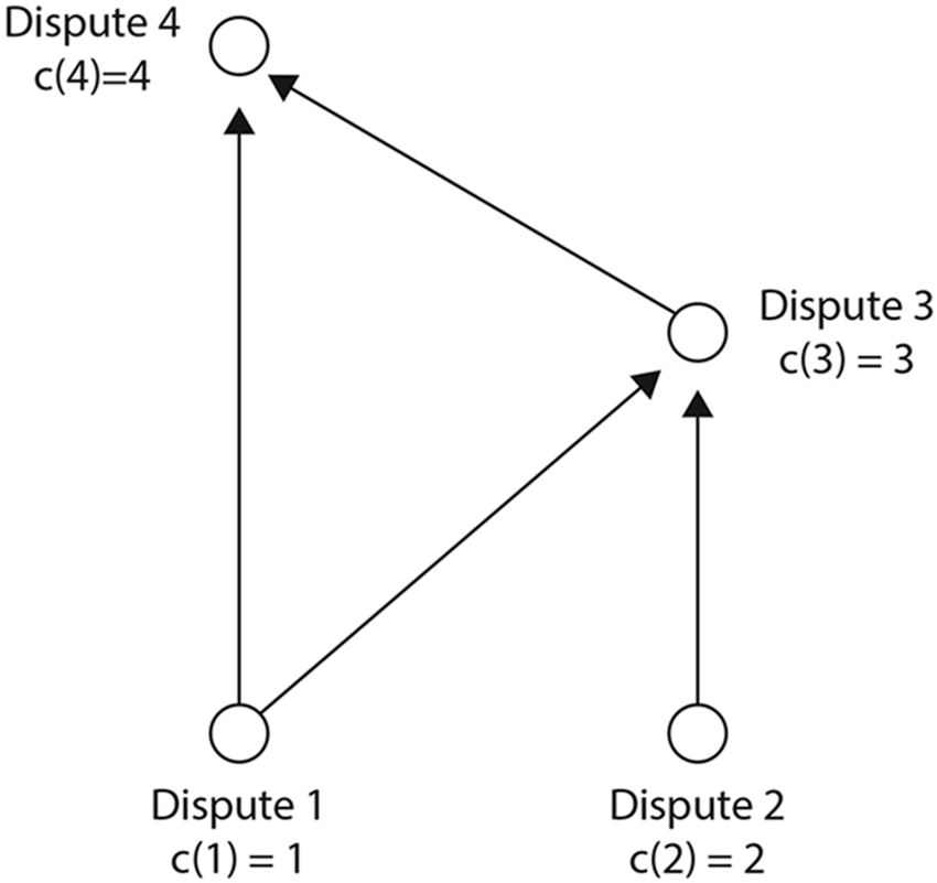
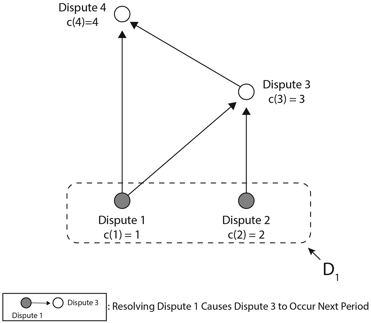
Example 1. Suppose that there are four potential disputes, $D = {1, 2, 3, 4}$ . The cost of delay for dispute 1 is 1, the cost of delay for dispute 2 is 2, the cost of delay for dispute 3 is 3, and the cost of delay for dispute 4 is 4 (i.e., $c (d) = d$ ). By assumption 1, the cost of adjudication, k, is less than 2: $k < 2$ . The linkages between the disputes are displayed in figure 1, where an arrow from one dispute i to another, j, indicates that resolving the dispute i in the first period will result in dispute j arising in the second period. In other words, the linkage matrix is

L = [\begin{matrix} 0 & 0 & 1 & 1 \\ 0 & 0 & 1 & 0 \\ 0 & 0 & 0 & 1 \\ 0 & 0 & 0 & 0 \end{matrix}] .

Figure 1.

Four-dispute example. Resolving a dispute can cause others to arise, as shown by arrows.

Note that disputes 1 and 2 are logically connected by dispute 3. Furthermore, dispute 2 is ancillary to dispute 1: while resolving dispute 2 raises dispute 3, resolving dispute 1 raises both disputes 3 and 4. Similarly, disputes 1 and 3 are logically connected by dispute 4, and dispute 3 is ancillary to dispute 1, but none of these facts play a role in this example.

We relegate the derivations of the optimal adjudication strategy to appendix B and instead focus here on comparing the optimal adjudication strategy for three different first-period dockets. Specifically, we consider the Court’s optimal behavior when, in the first period, it faces (i) only dispute 1 (i.e., $D_{1} = {1}$ ), (ii) only dispute 2 (i.e., $D_{1} = {2}$ ), or (iii) both disputes 1 and 2 (i.e., $D_{1} = {1, 2}$ ).

Court Faces Only Dispute 1 in First Period. When it faces only dispute 1 in the first period, the Court’s optimal adjudication strategy depends on the cost of adjudication, k. Resolving dispute 1 will trigger disputes 3 and 4 to be active in the next period.

Adjudication Is Inexpensive. When the cost of adjudication is very small ( $k < 1 / 2$ ), the Court should resolve dispute 1 in the first period and then resolve both disputes 3 and 4 in the second period. Why? Because in the second period the Court would resolve any dispute on the docket (since $k < 1$ ). As a result, the Court can wait to resolve dispute 1 and face a payoff of $−1 - k$ , or it can resolve dispute 1 in the first period and then resolve disputes 3 and 4 in the second period, which yields −3k.

Adjudication Is Moderately Costly. When the cost of adjudication is moderate (specifically, $1 / 2 < k < 1$ ), the Court should demur in period 1 and then resolve dispute 1 in the second period.

Adjudication Is Very Costly. When adjudication is very costly ( $k > 1$ ), the Court should demur in both periods and never resolve dispute 1.

Court Faces Only Dispute 2 in First Period. When the Court faces only dispute 2 in the first period, assumption 1 ensures that the Court should resolve dispute 2 in the first period and then resolve dispute 3 in the second period.

Court Faces Both Disputes 1 and 2 in First Period. When the Court faces both disputes 1 and 2 in the first period, the Court’s optimal adjudication strategy once again depends on the cost of adjudication, k.

Adjudication Is Inexpensive. When the cost of adjudication is sufficiently inexpensive ( $k < 1$ ), the Court should resolve both disputes 1 and 2 in the first period and then resolve both disputes 3 and 4 in the second period.

Adjudication Is Expensive. When adjudication is sufficiently costly ( $k > 1$ ), the Court should resolve dispute 2 in the first period and then resolve both disputes 1 and 3 in the second period.

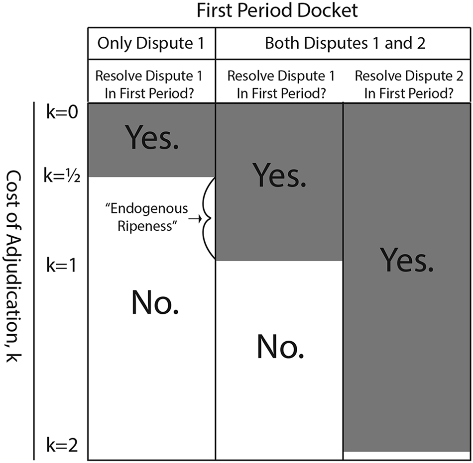
Figure 2 compares the optimal adjudication strategy when the first-period docket contains only dispute 1 with the optimal strategy when the docket contains both disputes 1 and 2. The figure illustrates what we refer to as “endogenous ripeness”: specifically, whenever the cost of adjudication is moderate ( $1 / 2 < k < 1$ ), the Court should resolve dispute 1 if and only if dispute 2 is also active in the first period. Dispute 2 is sufficiently costly to warrant resolution for all $k < 2$ . Because dispute 2 is logically connected to dispute 1, this implies that the net dynamic cost of resolving dispute 1 in the first period—that is, the net cost of dispute 1’s downstream consequences—is reduced when dispute 2 is resolved in the first period. Thus, assuming that the cost of adjudication is unobserved, the Court will be more likely to resolve dispute 1 when dispute 2 is also on the docket. QED

Figure 2.

Endogenous ripeness. If $1 / 2 < k < 1$ , then dispute 1 is resolved if and only if dispute 2 is also on the first-period docket.

Example 1 illustrates a core insight from our theory regarding how dynamic adjudication induces interdependencies between disputes. Note that when adjudication is moderately costly (i.e., $1 / 2 < k < 1$ ), dispute 1 is endogenously ripe. In a static (one-period) framework, the Court would optimally resolve dispute 1, because the cost of adjudication is less than the cost of not resolving the dispute. But, in a dynamic (two-or-more-period) framework, the downstream consequences of dispute 1’s successors will lead the Court to forgo resolving dispute 1. However, in a dynamic setting, the presence of dispute 2 on the docket restores the Court’s willingness to resolve dispute 1. Specifically, the presence of dispute 2 on the docket motivates the Court to also resolve dispute 1 in dynamic situations in which it would otherwise demur from resolving it.

B. Contingent Disputes

Dispute 1 in this example is a specific instance of what we term a contingent dispute. A dispute is contingent if its resolution is contingent on the other disputes on the docket: it will be resolved in some dockets but not others. That is, it is sometimes, but not always, optimal for the Court to leave a contingent dispute unresolved. Note that our assumption about adjudication costs (assumption 1) ensures that the Court would resolve every dispute if all of the disputes were pending at once, so the notion of a contingent dispute essentially identifies disputes that are not sufficiently important to always warrant immediate resolution.

Definition. A dispute is contingent if there is some docket containing it in which it is optimal for the Court to leave it unresolved in the first period and another docket containing it in which it is optimal for the Court to resolve it in the first period.

Given that the Court is omniscient in our theory, “learning” by the Court plays no explanatory role. Thus, the fact that contingent disputes exist in our setting implies that delay can emerge for strategic reasons completely independent of learning (e.g., Perry Reference Perry1991; Clark and Kastellec Reference Clark2013). Similarly, our Court is not collegial: it is a unitary actor making decisions in isolation. Thus, our theory provides an understanding of why delay might occur that is independent of motivations such as collegiality on the Court, deference by the Court to other political actors, or a desire to wait for coordination by lower courts (e.g., Caldeira and Wright Reference Caldeira1988; Perry Reference Perry1991; Epstein and Knight Reference Epstein1998; Lax Reference Lax2003).

Proposition 1. A dispute $d ∊ D$ is contingent if and only if

\begin{matrix} (3) & c (d) < k (1 + \frac{| S_{L} (d) |}{2}) - \min [k, c (d)] . \end{matrix}

The condition in proposition 1 (inequality [3]) yields a few immediate conclusions.

1. In line with our focus on the impact of dynamic considerations, a dispute can be contingent only if it has successors. If a dispute has no successors (i.e., its resolution has no downstream consequences for the Court) then the optimality of its resolution is independent of both when it emerges and what other disputes are pending when it emerges.
2. It is optimal to allow a dispute to simmer only if the dispute is not too costly to leave unresolved. Intuitively, a dispute can be contingent only if it is not too pressing on its own.
3. Disputes that have more successors are more likely to be contingent. The condition expressed in inequality (3) is a necessary condition for the Court to consider what other disputes are pending when deciding whether to resolve a given dispute d. That is, if inequality (3) is not satisfied for a given dispute d, then the dispute is sufficiently costly to endure and has sufficiently few downstream consequences (i.e., |S_L (d)| is small) so that the Court should resolve the dispute whenever it arises.

When inequality (3) is satisfied, we see how the downstream consequences of a dispute affect whether a Court is willing to resolve that dispute in any period. Costly downstream disputes discourage resolution—even if the dispute in question would be easy to resolve. However, the adverse side of those downstream consequences can be mitigated when there are other pending disputes that have the same downstream consequences. As our example illustrates, the cost-benefit balance is shifted as more cases with the same downstream consequences are presented, therefore not appreciably affecting the “cost” of resolving a dispute (i.e., triggering new disputes) while increasing the cost of demurring (i.e., leaving even more pending disputes unresolved).

Result 1. Expectations about what an adjudicator will (or will not) have to adjudicate in the future will affect its willingness to let a dispute percolate.

There are many reasons why a rational judge might choose to wait before resolving a given dispute. He may want to allow the issue to percolate more to gain more information, or he may want to await a favorable ideological climate or allies on the Court. We show that even in the absence of ideological considerations and even when a judge has complete information, he still may prefer to wait. This is because there is a benefit to minimizing the total cost of pending, live questions.

C. Dynamically Induced Resolution Interdependence

Example 1 demonstrates that the dynamic relationships between potential disputes can induce interdependence in the Court’s optimal approach to dispute resolution. That is, when two disputes are logically connected through their downstream consequences, the Court might not resolve either of them unless both of them are active. This is easily illustrated by a simple example.

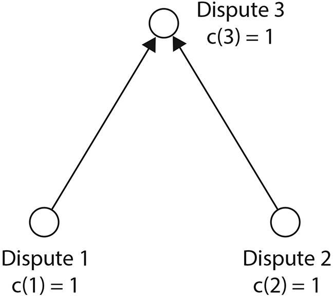
Example 2. Consider the three-dispute example illustrated in figure 3, where all three disputes are equally costly to endure, and two of the disputes each initiate (and are hence logically connected through) the third dispute.Footnote ¹⁴ Assumption 1 implies that the cost of adjudication is less than 2 ( $k < 2$ ). If this cost is large enough ( $k > 1$ ), then it is not optimal to resolve dispute 1 if it is the only active dispute in the first period. The symmetry of the example means this is true for dispute 2 as well. In such a situation, the Court should never resolve the dispute. However, if both disputes are active in the first period, then the fact that $k < 2$ implies that it is optimal to resolve both disputes, after which the Court should resolve dispute 3 in the second period if $k < 1$ . QED

Figure 3.

Simple example of resolution interdependence

Example 2 illustrates a key result of our framework: the question of whether resolution of one dispute is optimal can depend on what other disputes are pending, and, furthermore, this dependence can emerge from logical connections between the disputes in terms of their downstream implications. That is, even if the disputes appear unrelated, their future consequences might induce a connection between them with respect to whether their joint or severable resolution is optimal. We now turn to an even stronger result that leverages the nature of the downstream linkage of the disputes in question.

D. Ancillary Disputes

The next result further illuminates the nature and origins of the interdependence of optimal resolution created by disputes’ dynamic relationships. In particular, proposition 2 states that if it is optimal to resolve a dispute d in any given initial docket, then it is also optimal to simultaneously resolve any disputes ancillary to d.Footnote ¹⁵

Proposition 2. Suppose that dispute a is ancillary to d. If (1) both a and d are active in the first period and (2) it is optimal to resolve d, then it is optimal to also resolve a.

The monotonicity established in proposition 2 reveals a crucial source of static interdependence that arises from dynamic linkages. Two disputes that seem unrelated today may be connected by shared offspring. As a result, the decisions to resolve seemingly independent disputes may not be independent. In particular, judicial decisions and interpretations are relevant to the Court at least partially because the Court will have to revisit them in the future. Accordingly, the Court’s consideration of what future cases will or will not arise can affect its willingness to let even a seemingly pressing issue percolate. Put more directly, our analysis illustrates the interdependence (or “joint dependence”) of the Court’s optimal adjudication strategy on the combination of various disputes eligible for resolution.

Result 2. A strategic adjudicator will resolve (weakly) more disputes as the number of pending disputes increases.

E. Downstream Consequences and Endogenous Economies of Scale

In line with our discussion of proposition 1, whether a contingent dispute should be resolved is a function of how much overlap there is in the downstream consequences of logically related disputes. Proposition 2 demonstrates a strong result that, if a disputes’s downstream consequences are totally subsumed by another dispute (i.e., if a dispute is ancillary to another pending dispute), then it is optimal to resolve that ancillary dispute whenever it is optimal to resolve the other dispute.

One of the richer results that arises from that relationship is a form of an endogenous economy of scale. Even while we assume constant, linear costs to adjudicating disputes, economies of scale arise endogenously in the dynamic resolution framework. This may produce “episodic” or “burst” style adjudication, in which the Court decides related cases in clusters. These economies arise because of the common downstream consequences that follow from resolving any given collection of disputes. Consider an illustrative example.

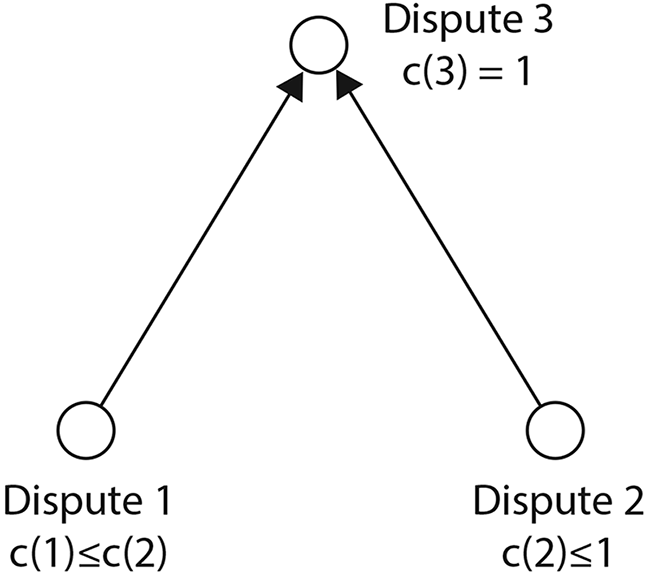
Example 3. Consider the generalization of the three-dispute setting from example 2 pictured in figure 4. Suppose that dispute 3 is not active in the first period. The optimal resolution strategy depends on the cost of adjudication. The four relevant circumstances are described below.

1. $k < c (1) < c (2) < 1$ : In this case, it is always optimal for the Court to resolve dispute 1 or dispute 2 or both if either or both are active in the first period.
Figure 4.
Endogenous economies of scale
2. $c (1) < k < c (2) < 1$ : For moderately low adjudication costs, it is optimal for the Court to resolve dispute 1 if and only if dispute 2 is also active, in which case it is optimal to resolve both disputes in the first period and then resolve dispute 3 in the second period. Otherwise, the Court should leave dispute 1 unresolved in both periods.
3. $c (1) < c (2) < k < 1$ : When adjudication costs are moderately high, it is optimal for the Court to resolve dispute 1 if and only if
1. a) dispute 2 is also active and
2. b) the sum of the costs of enduring disputes 1 and 2 is sufficiently large:Footnote ¹⁶
  $c (1) + c (2) > \frac{3 k}{2} .$

If both of these conditions hold, then the optimal resolution strategy is to resolve both disputes 1 and 2 in the first period and then resolve dispute 3 in the second period. If either or both do not hold, then it is optimal for the Court to resolve no disputes in either period.

4. $c (1) < c (2) < 1 < k$ : When adjudication costs are sufficiently high, then it is optimal for the Court to leave both dispute 1 and dispute 2 unresolved in both periods.

For moderate adjudication costs ( $c (1) < k < 1$ ), the optimal resolution of dispute 1 depends on both whether dispute 2 is active and whether the Court resolves it in the first period (there is no situation in which the Court resolves dispute 1 while leaving dispute 2 active and unresolved). Furthermore, the fact that optimal dispute resolution depends on the sum of the costs of enduring disputes 1 and 2 for moderately high adjudications ( $c (2) < k < 1$ ) represents a form of an economy of scale: the optimal resolution of dispute 1 depends on characteristics of (i.e., the cost of not resolving) dispute 2. QED

Example 3 highlights not only the potential importance of what disputes are logically connected to each other—a point that follows from the discussion of downstream consequences—but also the costliness of allowing each of the logically connected disputes to remain unresolved. If a given dispute is logically connected to other disputes that are costly to endure, the dispute in question will be more likely to be resolved than if it is logically connected to less costly disputes. Analogously, if one holds fixed a dispute’s downstream consequences (i.e., its set of successors), resolution of that dispute becomes more likely as the set of disputes to which it is logically connected grows: enlarging the number of logical connections of a given dispute will increase the Court’s incentive to resolve that dispute.

Result 3. Logical connections among cases affect their net downstream consequences. As a case becomes logically connected to a larger set of cases, the Court will become more likely to resolve that dispute, endogenously creating the appearance of an economy of scale in adjudication.

The above is one empirical prediction of our model: the likelihood of speedy resolution should be higher for cases that are more connected. Proposition 1 offers another empirical prediction. From that proposition, a dispute can only be contingent if it has successors. Disputes with no successors are resolved either immediately or never. Therefore, in our theory, all cases that are allowed to percolate must have progeny. Moreover, whenever a court resolves a case that has percolated, it will also resolve one or more cases that share some or all of that case’s progeny. In this way, those cases that are allowed to percolate will always be followed by clumpy resolution. This empirical prediction distinguishes our model from theories of percolation for retrospective reasons like learning. In our model, delay occurs because progeny are ready, so cases that have been allowed to percolate will always be decided in a clumpy fashion. We summarize this empirical prediction below.

Result 4. Only those cases with downstream consequences are delayed and, whenever a court allows a case to percolate, it will decide that case and one or more other cases with common progeny.

F. Summary of Theoretical Predictions

Our model yields a variety of insights into how disputes ought to be resolved across time when cases have known downstream consequences. First, the Court may prefer not to resolve a dispute today if resolution would raise too many costly subsequent disputes. Second, optimal dispute resolution depends on the relationships between pending disputes: when two or more disputes are linked to one or more subsequent disputes, the Court’s optimal resolution of any of those disputes may depend on both whether the other disputes are pending and their characteristics, including both how costly the disputes are to endure as well as how much their downstream consequences overlap. Thus, even though we assume a linear cost of adjudication, there is an apparent economy of scale in optimal resolution: related disputes are more likely to be resolved together. Substantively, even if the Court does not formally consolidate cases for resolution and hears each on its own, there is still cost savings by resolving multiple disputes together. We now illustrate a key result from our theoretical analysis, using a case study from the US Supreme Court.

V. Historical Example: Downstream Consequences and Readiness for Resolution

We illustrate the dynamic of “delaying the problem” with the use of statistics as evidence in judicial proceedings. Lawyers have offered statistical evidence in litigation since at least the mid-19th century, but courts have established doctrines guiding the use of statistics only very recently. As early as 1868, in Robinson v. Mandell (20 F. Cas. 1027)—a case concerning handwriting analysis that is regarded as the first attempt to present statistical evidence in court (Barnes and Conley Reference Barnes1986, 5)—Circuit Justice Clifford wrote, “Some of the questions discussed were new, and it must be admitted that they are highly important as affecting the rules of evidence.” But beginning to outline a doctrine on when and how statistics constitute evidence would have raised too many difficult follow-up questions, so Justice Clifford declined to prescribe any doctrine for using statistical evidence. In fact, it was almost 100 years before these questions regarding the use of statistics as evidence were answered. That century saw a dramatic increase in the use of statistics in court, driven in large part by developments in the social sciences and the rise of behavioral sciences more generally. By the 1950s and 1960s, social-scientific approaches and statistical evidence were popular (e.g., social science experiments were famously presented in Brown v. Board of Education), and the high cost of not having a doctrine on the use of statistics was clear. Despite these costs, the Court procrastinated about issuing a doctrine on the use of statistics. So, the use of statistics in court was increasingly frequent but suspect, and very little law governed its use (Fienberg Reference Fienberg1989, 6–7). Our model provides a theoretical foundation for why the Court tolerated this century-long ambiguity: it realized that the resulting ambiguity from issuing a doctrine would be even more severe. If the Court issued a doctrine on when statistical evidence could be admitted, resulting questions on what qualified as statistical evidence, what qualified as statistical significance, and so on, would overwhelm the courts.

Beginning in the 1970s, there was a “sharp increase” in the use of statistics in court (Fienberg Reference Fienberg1989, 211). That sharp increase was not itself driven by a demand for doctrine on statistical evidence (at least not directly). Rather, the increase can be attributed to progressive legislation such as the Equal Pay Act of 1963 and the Civil Rights Act of 1964, which created legal questions about how to prove discrimination (Kuhn Reference Kuhn1987). This abundance of cases provided the Court with the opportunity to bundle separate examples of statistical evidence together and resolve these seemingly separate disputes at once. The Court knew resolution of any of these would raise clarifying questions, and it knew these clarifying questions would still be difficult and plentiful. But now multiple questions raised similar clarifying questions, thereby offering an economy of scale. The Supreme Court took advantage of this opportunity when, in its 1971 decision of Griggs v. Duke Power Co., it noted that a test was discriminatory in part because it had the effect of “disqualify[ing] Negroes at a substantially higher rate than white applicants.” Although it dealt minimally with the statistical evidence underlying that claim, its decision quietly “opened the door to statistical proof” (Barnes and Conley Reference Barnes1986, 10). As expected, the Court’s decision in Griggs invited further disputes. These subsequent disputes included how to identify exactly when statistical evidence is admissible, exactly when it is proof of discrimination, and how it should be treated by the various actors in the judicial process. We argue that the Court foresaw these interconnected disputes and waited until it could answer many at once.

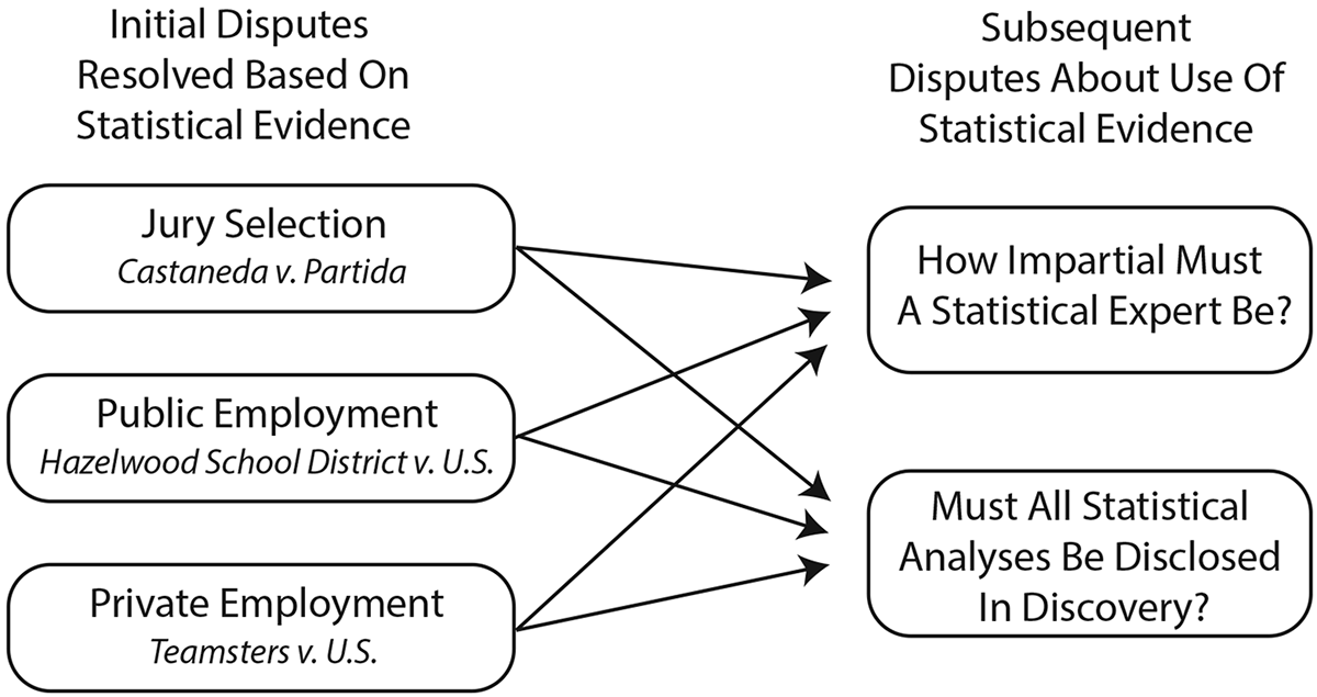
If the Court decides statistics are valid evidence in employment discrimination cases, subsequent disputes naturally arise—what the appropriate reference group is, whether such evidence is fully supportive on its own or whether it should be buttressed with evidence specific to the case at hand. But these questions also arise for other kinds of discrimination—jury selection, school composition, and so on. In 1977, the Court addressed the admissibility of statistical evidence in three decisions on discrimination: Castaneda v. Partida, Teamsters v. United States, and Hazelwood School District v. United States. These cases established the principles for using statistics to demonstrate discrimination in jury selection, employment and union practices, and hiring practices, respectively. By corralling these three cases, the Court was able to resolve a collection of questions about what kinds of legal claims can be made with statistical evidence. However, as we depict in figure 5, resolving those cases gave rise to subsequent issues that had to be worked out. For example, what constitutes statistical significance? In 1983, exemplifying the costs of leaving such a question unresolved, the Fourth Circuit wrote that “the Supreme Court itself, though disclaiming any intention ‘to suggest that precise calculations of statistical significance are necessary in employing statistical proof,’ has stated that standard deviations of more than ‘two or three’ represent a minimum for statistical significance” (E.E.O.C. v. Federal Reserve Bank of Richmond, 698 F.2d 633). These, and many other, questions were made more pertinent by the Supreme Court’s three 1977 decisions. Because doctrine on the use of statistics is always relevant to many different areas of law, the Supreme Court’s wariness to provide an overarching doctrine on the use of statistics continues today. In 2016, in Tyson Foods, Inc. v. Bouaphakeo (136 S.Ct. 1036), the Supreme Court ruled that “the Court would reach too far were it to establish general rules governing the use of statistical evidence, or so-called representative evidence, in all class-action cases. Evidence of this type is used in various substantive realms of the law. Whether and when statistical evidence can be used to establish classwide liability will depend on the purpose for which the evidence is being introduced and on ‘the elements of the underlying cause of action’” (internal citations omitted).

Figure 5.

Linkages among cases involving statistical evidence. Left, set of cases concerning the types of claims of discrimination for which statistical evidence can be presented. Right, subsequent issues that arose about how to evaluate and handle statistical evidence in a trial.

Our model illustrates the cautionary effect of foresight (in result 3 and example 1). We show too that once the Court decides to resolve a dispute, it will “sweep up” many logically connected, ancillary disputes. Empirically, once the Court decided to set a standard for using statistics to show discrimination, it collected all of the then-pending questions (jury discrimination, employment discrimination, and jury selection) and resolved them virtually at the same time. Allowing statistical evidence to establish a prima facie case for discrimination would allow the Court to resolve the cases at hand, but it would raise further (and more technical) questions about what kinds of statistical evidence should suffice. In 1868, when the Court first had the opportunity to address the use of statistics in court, the costs of resolving these ancillary questions arguably outweighed the tiny set of other disputes from which the Court would gain from resolving them. But by the late 1970s, the ancillary questions were implicated in a sufficiently large number of pressing cases about statistical evidence that the Court found it worthwhile to raise them.

VI. Assumptions and Extensions

By design, our theory is centered on one particular aspect of dynamic adjudication—namely, how the Court should compare the downstream consequences of resolving a dispute against the cost of delaying resolution. This focus necessarily sets aside several other dynamic considerations. For example, one might expect delay to emerge either from allowing cases to percolate in order to learn more about the underlying dispute or in an attempt to take advantage of the most favorable ideological climate. Omitting these very real possibilities is part of the power of our results, indicating that delay in adjudication need not imply that the Court is motivated by such considerations: rather, the Court might delay based solely on the factors at play in our theory.

Focusing only on the consideration of downstream consequences as captured in our theory, there are several paths for further development. For example, questions left unresolved by a court might create political incentives for a legislature to take up the issue, thereby creating an alternative set of dynamic costs associated with delay. Complementarily, resolving a dispute might “take the wind out” of a politically salient policy debate: resolving a dispute may remove future disputes from the docket. These possibilities, which we expand on below, are intriguing and present promising future extensions to the model; our framework can naturally handle them.

A. Costly Resolution

We assume that resolving a case is costly to the Court, but one might suppose that the Court also benefits from resolving a dispute. The most natural situation in which this might shape our analysis is when a dispute itself has a large net benefit to being resolved but triggers an arbitrarily large set of successor disputes. Allowing the Court to directly enjoy resolving a dispute would not change our qualitative results as long as there are some disputes that the Court finds costly to resolve.Footnote ¹⁷ For those cases the Court wants to resolve that trigger a large number of costly successor disputes, the same dynamics we describe in this article would apply—the Court would face an incentive to demur in order to avoid the large downstream consequences. Were enough other disputes to arise with shared downstream consequences, that incentive would be mitigated, and the Court might consider resolving the initial dispute. We anticipate that an extension of this model could directly incorporate this possibility.

B. Strategic Litigation

Our model abstracts from the role of litigants in bringing cases and setting the Court’s docket, but research suggests that signals sent by litigants can communicate to the Court the importance of a given case (e.g., McGuire and Caldeira Reference McGuire1993; McGuire Reference McGuire1994; Boucher and Segal Reference Boucher1995; Spriggs and Wahlbeck Reference Spriggs1997). Our framework has implications for how interested, potentially strategic, litigants can influence the mix of issues available for resolution at any given time. While our theory is deliberately stark and omits consideration of strategic litigants and other actors—the theory considers only the incentives of a court facing a set of disputes with exogenous linkages—it provides the theoretical underpinnings for a fuller consideration of the incentives such actors would face.

If the Court is sensitive to the anticipated consequences of resolution—even of resolution of another dispute—then litigants might increase the likelihood their case is heard by manipulating the whole docket over time. A variety of questions in political science concerning distributive politics are implicitly motivated by this concern, most notably in the study of the development of rights through litigation (e.g., Epp Reference Epp1998; Sanders Reference Sanders1999; Kersch Reference Kersch2004). Moreover, this type of strategy is not just a feature of long trends in special interest litigation. Administrative agencies specifically identify the links among cases as a component of their strategic calculus. An Organization for Economic Cooperation and Development report on competition between the US Federal Trade Commission and the Department of Justice notes, “The Commission sometimes brings cases not only because of the immediate market impact, but also because the case may help clarify the law. … The value of enforcement action goes beyond the specific case by clarifying the law and in turn guiding the broader business community” (1999, 5).

In this article we assume that the initial docket is exogenous and that subsequent dockets are a function of strategic choices made only by the Court. In reality, the probabilistic connections among cases are a rich strategic game involving litigants, courts, and special interests, among other actors. Future extensions to the modeling framework could consider how actors such as interest groups, lower courts, executives, and legislatures might use their various tools (e.g., lawsuits, interpretation of precedent, prosecutions, and legislation) to create and alter links between current and future disputes. In a sense, while our theory is merely one of many ways in which issue linkages can be conceptualized, a framework such as the one we provide is arguably necessary for any full theoretical treatment of how phenomena such as issue networks emerge (Heclo Reference Heclo1978), as well as understanding more generally how and why interest groups attempt to tie issues together when lobbying legislatures and the public (Baumgartner and Jones Reference Baumgartner1993, Reference Baumgartner2009; Baumgartner and Leech Reference Baumgartner and Leech1998, Reference Baumgartner and Leech2001; Hurwitz, Moiles, and Rohde Reference Hurwitz2001).

C. Strategic Opinions: Control of the Linkage Matrix

In our model, we assume the links among cases are exogenous and fixed. However, there are certainly factors that shape and condition the links among cases. Just as the dockets that arise are presumably a function of strategic behavior, it is reasonable to suppose that the linkage between disputes—the downstream implications of dispute resolution—is also the product of strategic behavior. From an empirical standpoint, the Court has some control over the scope and nature of the downstream implications of its decision (e.g., how it crafts its opinion may limit or expand the scope of the decision). We do not explicitly model this possibility mostly because of space constraints: we would need to add additional assumptions about the constraints on the Court’s ability to delimit the downstream consequences of its own decisions.Footnote ¹⁸

Without venturing into such an exercise, however, our framework does provide some strong suggestions about the Court’s incentives: it wants to limit the downstream consequences of any dispute it resolves as much as it can. This is broadly in line with the principles of judicial minimalism, or “one case at a time” judging, which (in slightly different ways) call on the Court to limit the scope of its rulings as much as possible. By demurring from considering even intimately related issues that are unnecessary for the disposition of the pending dispute, the Court curtails the downstream consequences of its resolution.Footnote ¹⁹ A promising angle on empirically validating the utility of our framework in describing judicial decision making would be to probe whether and how downstream consequences of a decision inform how justices (and clerks) draft opinions and decide whether to accept cases brought to the Court.

D. The Punctuated Nature of Policy Making

Our results show that legal questions raised as matters ancillary to more important questions will be resolved sooner than otherwise similar issues that are connected to less important questions. Our theoretical framework provides an understanding for why dispute resolution can appear “clumpy” as a result of the Court not resolving any seemingly pressing issues in a domain for a significant period of time and then, in one fell swoop, resolving a host of related issues. More specifically, the theory provides an explanation for this behavior that does not depend on the importance of the pending issues varying across time. Rather, the key causal mechanism in our theory is the emergence of a sufficient number of disputes with common downstream consequences.

This helps us to understand two ubiquitous, but seemingly contradictory, attributes of political processes within mature institutions—“a plethora of small accommodations and a significant number of radical departures from the past” (Baumgartner, Jones, and Mortensen Reference Baumgartner2014, 60). Punctuated equilibrium theory explains the coexistence of these phenomena by emphasizing issue definition and agenda setting and by arguing that “reinforcement creates great obstacles to anything but modest change, whereas questioning policies at the most fundamental levels creates opportunities for major reversals” (60). Our theory complements this tradition. In particular, our theory explains both stasis and “punctuations” in a single framework, but it does so without relying on ancillary concepts such as bounded rationality or limited attention.Footnote ²⁰ Our theory’s complementary perspective is based on the interactive effect of both foresight—some disputes should be delayed while awaiting others to “play out”—and the possibility that multiple decisions might have common dynamic effects. These dynamic interconnections are the key to our theory’s prediction of periods of relative quiet being interrupted intermittently by bursts of multiple decisions at once.

VII. Discussion and Conclusion

Doctrinal development is a strategic, dynamic, path-dependent process. Scholarship on policy making has documented the strategy behind sequential steps taken in the crafting of individual policies and also the long-run sequential nature of political movements that encompass many individual policy achievements. Likewise, scholarship on judicial decision making has recognized that courts often delay resolution of seemingly important issues. We unify these perspectives within a model of dynamic dispute resolution. The model allows us to consider the implications of foresighted judging, yielding implications about how a strategic judge will sequence various questions posed in light of the salience or import of the questions and especially the interlinkages among the various questions.

A. Noninformational Percolation

Much has been written about why courts, especially the US Supreme Court, demur from resolving seemingly pressing questions. Some normative theorists (e.g., Bickel Reference Bickel1962; Ely Reference Ely1980; Sunstein Reference Sunstein1999) contend that courts should avoid answering too many questions, in order to leave as much authority as possible in the hands of more democratically accountable institutions. Other researchers have argued that courts need to allow issues to percolate in order to observe how disputes play out and thereby learn what resolution is best suited to the problem (e.g., Tiberi Reference Tiberi1993; Clark and Kastellec Reference Clark2013). Still others claim that it is too demanding to select which disputes to resolve and how much effort to put into any given question, so courts must rely on cues from the political world to navigate the mass of disputes that come before them (e.g., Caldeira and Wright Reference Caldeira1988). Our model demonstrates that courts might allow issues to percolate and remain unresolved even absent any of these concerns. By enduring an unresolved dispute, a court might forestall significant downstream consequences, such as a flood of new questions or issues. Indeed, it is a common understanding in the literature on litigation—especially concerning the definition of rights—that, once the Supreme Court wades into an issue area, it often provokes a series of new questions implied by its resolution of the initial dispute.

B. Connected Disputes and Strategic Dilemmas

American courts make policy only through the adjudication of individual cases. They cannot articulate rules ad hoc: courts establish rules through the individual cases they hear and through analogies among them (e.g., Fox and Vanberg Reference Fox2014; Callander and Clark Reference Callander2017). If a court must make policy through cases, what constitutes a good case by which to articulate a doctrine or rule? Much theoretical research interrogates which cases the Supreme Court chooses to review, but that work typically focuses on case-level, static factors that make disposing of the individual case appealing. (Such factors include the ideological relationship to the lower court, the composition of the current court, signals like dissents or briefs that indicate a case’s importance, or the relationship to the broader political sphere; see, e.g., Cameron, Segal, and Songer Reference Cameron2000; Lax Reference Lax2003; Clark Reference Clark2009; Beim, Hirsch, and Kastellec Reference Beim2014.) Our analysis reveals that dynamic considerations—specifically the anticipated path of disputes—can make seemingly equal disputes more or less attractive vehicles for policy making. The consequence is that a description of agenda setting, including a study of certiorari, is complete only if it considers dynamic linkages among disputes.

Appendix A: The General T-Period Model

We present here a more general formulation of our theoretical framework in which the number of time periods is arbitrary but finite. That is, in the setting presented here, the Court adjudicates disputes across $T \geq 1$ discrete periods, where T is finite (but may be arbitrarily large).

Disputes and Linkages

Each dispute d is characterized by a dispute-specific cost of delay, $c (d) \geq 0$ . We focus on dynamic linkages between disputes—that is, which subsequent disputes any given dispute will provoke and which other disputes will provoke those same follow-ups—and seek to understand how these dynamic linkages affect the incentives of the Court to resolve any given dispute. The set of all n possible disputes is denoted by $D$ . The (exogenous) linkages between disputes are represented by an $n \times n$ linkage matrix, L. The probability that resolving dispute d will provoke some dispute j is denoted by $L_{dj} ∊ [0, 1]$ , with the additional restriction $L_{dd} = 0$ : resolving any given dispute does not (immediately) lead to the recurrence of that dispute. Thus, L defines a weighted graph on $D$ . In order to keep presentation as parsimonious as possible, we focus on the case in which linkages are deterministic: $L_{dj} ∊ [0, 1]$ for each distinct pair of disputes d and j. Part of the reason this decision makes the presentation parsimonious is that it allows us to unambiguously refer to the “predecessors” and “successors” for any dispute $d ∊ D$ , given the linkage matrix L. The predecessors of a dispute d, denoted by P_L (d) are those disputes that, when resolved, provoke dispute d:

P_{L} (d) = {j ∊ D : L_{jd} = 1},

and the successors of a dispute d, denoted by S_L (d), or simply S(d), are those disputes that are provoked when d is resolved:

S_{L} (d) = {j ∊ D : L_{dj} = 1} .

Sequence of Play and the Court’s Payoffs

At the beginning of each period t, the Court observes the (possibly empty) set of disputes that are available for resolution, $D_{t} \subseteq D$ . We call D_t the Court’s docket. Following observation of D_t , the Court can adjudicate as many available cases as it wants. We assume that the direct cost of adjudication is a linear function of the number of cases adjudicated: if the Court adjudicates x cases, it pays a direct cost of kx, for $k \geq 0$ .Footnote ²¹ The set of cases the Court adjudicates in period t is denoted by $a_{t} \subseteq D_{t}$ , and the set of cases remaining to be disposed of is denoted by $r_{t} \equiv D_{t} \ a_{t}$ . The payoff received by the Court in period t is

U_{t} (a_{t}; D_{t}) = - [k | a_{t} | + \sum_{d ∊ r_{t}} c (d)] .

The next docket—the set of cases available for resolution in period $t + 1$ —consists of those cases that were available for resolution, but not resolved, in period t ( $D_{t + 1} = r_{t}$ ) and all cases provoked by those resolved in period t (except those that would have been provoked but were resolved in period t—we assume these do not immediately reappear).Footnote ²² Thus, the probability that dispute j is in $D_{t + 1}$ , given D_t and a_t , is denoted and defined by

P (j; D_{t}, a_{t}) \equiv {\begin{matrix} 0 & if ∊ j ∊ a_{t}, \\ 1 & if j ∊ r_{t}, \\ 1 - \prod_{d ∊ a_{t}} (1 - L_{dj}) & otherwise . \end{matrix}

Thus, given D_t and a_t , the probability that the next period’s docket will equal D is

P (D; D_{t}, a_{t}) \equiv \prod_{d ∊ D} P (d; D_{t}, a_{t}) \prod_{j \int D} (1 - P (j; D_{t}, a_{t})),

or, given our restriction of attention to deterministic linkage matrices, the next period’s docket is with certainty given by

D_{t + 1} (D_{t}, a_{t}) = r_{t} \cup (\cup_{d ∊ a_{t}} S_{L} (d)) \ a_{t} .

Then, for any T-period sequence of dockets, $D = (D_{1}, \dots, D_{T})$ , and adjudications, $a = (a_{1}, \dots, a_{T})$ , the Court’s overall payoff is simply

(A1)

\begin{matrix} (A1) & U (a; D) = \sum_{t = 1}^{T} δ^{t - 1} U_{t} (a_{t}; D_{t}), \end{matrix}

where $δ ∊ (0, 1]$ is an exogenous discount factor. Finally, a setting, $σ = (D, c, k, L)$ , is a combination of a set of $n \geq 1$ potential disputes, $D$ ; a vector of costs of delay, $c ∊ R_{+ +}^{n}$ ; a cost of adjudication, $k \geq 0$ ; and a $n \times n$ matrix of linkages, L. The set of all potential settings is denoted by Σ.

Adjudication Strategies

A T-period adjudication strategy is a complete description of which disputes will be resolved and when they will be resolved. Specifically, for any setting σ and number of time periods T, an adjudication strategy is a mapping, denoted by $α : 2^{D} \times {1, \dots, T} \to 2^{D}$ , that maps each docket, $D \subseteq D$ , and the time period, $t \subseteq {1, \dots, T}$ , into a set of disputes to resolve, denoted by α(D,t).Footnote ²³ The set of all adjudication strategies, given a setting σ and a number of time periods T, is denoted by $A (σ, T)$ . For any setting σ, number of time periods T, and initial docket $D_{1} \subseteq D$ , an adjudication strategy $α ∊ A (σ, T)$ induces, for each time period $t ∊ {1, \dots, T}$ , a distribution of dockets and adjudication decisions.

Given a setting σ, a time horizon T, a discount factor δ, and an initial docket $D_{1} \subseteq D$ , we denote the Court’s total payoff from an adjudication strategy $α ∊ A (σ, T)$ by EU(α;σ, T, δ, D ₁).Footnote ²⁴ With this in hand, an adjudication strategy $α^{*} ∊ A (σ, T)$ is optimal for any setting σ, number of time periods T, and discount factor δ, if it maximizes EU(·; σ, T, δ, D ₁) for each possible initial docket $D_{1} \subseteq D$ :

(A2)

\begin{matrix} (A2) & \forall D_{1} \subseteq D, ∊ α^{*} ∊ \underset{α ∊ A (σ, T)}{argmax} ∊ EU (α; σ, T, δ, D_{1}) . \end{matrix}

We denote the set of all optimal adjudications for a setting–time length pair (σ,T) by $A^{*} (σ, T, δ)$ . When the setting σ is clear, we denote the set of all t-period optimal adjudications in period $t \leq T$ for any docket $D \subseteq D$ by $A_{t}^{*} (D)$ . We show later that the set of optimal adjudication strategies is nonempty and generically unique (proposition 4).

While our existence result applies to any finite time horizon, much of our discussion in the article focuses on the two-period setting ( $T = 2$ ). It is important to note that this simplification is merely for presentational purposes. The two-period setting is sufficient to highlight the Court’s incentives in a dynamic adjudication setting, and our findings extend to any finite horizon setting with more than two periods.Footnote ²⁵

Analysis

Assumption 2. Given the discount factor, δ, each dispute $D ∊ D$ satisfies

c (d) > \frac{k}{1 + δ} .

Assumption 2 establishes a useful baseline: any dispute in the initial docket that is left unresolved by an optimal strategy is left unresolved precisely because of the dynamic implications of its resolution. That is, given assumption 2, an optimal adjudication strategy would resolve all disputes in the first period in a “static” setting, where the linkage matrix, L, contains only zeroes.

Dynamically Induced Dispute Interdependence

Our model demonstrates that dynamic relationships create interdependence among cases being considered by the Court at the same time. This result, as we show below, has direct implications for theoretical and empirical models of case selection and agenda setting.

We begin by defining connectedness among cases. One such notion is similar to covering or domination (Fishburn Reference Fishburn1977; Miller Reference Miller1980; McKelvey Reference McKelvey1986) and emerges when one dispute initiates a strict superset of the disputes initiated by another dispute to which it is logically connected. In this case, resolution of the first dispute renders mute the dynamic implications of resolving the second dispute. Formally, when one dispute’s successors are contained within those of another dispute with which it is logically connected, the first dispute is said to be ancillary to the second.

Definition. Given a setting $σ = (D, c, k, L)$ , and any pair of disputes $d_{1}, d_{2} ∊ D$ that are share a common successor, d ₁ is ancillary to d ₂ if $S_{L} (d_{1}) \subseteq S_{L} (d_{2})$ .

The relationship is referred to as ancillary because, if d ₁ is ancillary to d ₂, then resolving dispute d ₂ initiates every dispute that resolution of d ₁ would initiate. Note that two disputes can be ancillary to each other: this occurs when the two disputes have identical successors.Footnote ²⁶

With our definition of ancillary disputes, our next result provides further insight into the static interdependence created by disputes’ dynamic relationships. In particular, proposition 3 states that if it is optimal to resolve a dispute d in any given initial docket, then it is also optimal to simultaneously resolve any disputes ancillary to d. This is a dominance argument, but it also establishes a specific monotonicity result: when one adds an ancillary dispute, it remains optimal to resolve the original dispute, and it is optimal to resolve the ancillary dispute as well.

Proposition 3. For any setting $σ = (D, c, k, L) ∊ Σ$ , any positive integer T, any discount factor δ, and any T-period optimal adjudication $a^{*} ∊ A^{*} (σ, T, δ)$ , if $d ∊ D$ is ancillary to $d^{'} ∊ D$ , then for any $D \subseteq D$ with ${d, d^{'}} \subseteq D$ , $d^{'} ∊ a^{*} (D, 1)$ implies $d ∊ a^{*} (D, 1)$ .

It is straightforward to see that the converse of proposition 3 does not hold: if resolving a dispute is optimal in a docket and one adds a dispute to which that dispute is ancillary, it is not necessarily the case that resolving the newly added dispute is optimal, too—the newly added dispute might initiate an arbitrarily large number of disputes above and beyond those that the original dispute initiates.

Appendix B: Technical Results and Proofs

Derivations for Example 1

Suppose that there are four potential disputes, $D = {1, 2, 3, 4}$ . The cost of delay from each dispute $d ∊ D$ is given by $c (d) = d$ . That is, dispute 1’s cost of delay is 1, the cost of delay for dispute 2 is 2, the cost of delay for dispute 3 is 3, and the cost of delay for dispute 4 is 4. The cost of adjudication is $k < 1$ for each dispute. Furthermore, suppose that the set of initially available disputes is $D_{1} = {1, 2}$ and that the linkages between the disputes are as follows:

L = [\begin{matrix} 0 & 0 & 1 & 1 \\ 0 & 0 & 1 & 0 \\ 0 & 0 & 0 & 1 \\ 0 & 0 & 0 & 0 \end{matrix}],

so that the linkages are as displayed in figure B1, where an arrow from one dispute i to another, j, indicates that resolving the dispute i in the first period will result in dispute j arising in the second period.

Figure B1.

Endogenous ripeness

There are four potential adjudication decisions for the Court in the first period ( $a_{1} ∊ {Ø, {1}, {2}, {1, 2}}$ ), and the docket that the Court will face in the second period as a function of the first-period adjudication is given by

\begin{matrix} D_{2} (Ø) & = & {1, 2}, \\ D_{2} ({1}) & = & {2, 3, 4}, \\ D_{2} ({2}) & = & {1, 3}, and \\ D_{2} ({1, 2}) & = & {3, 4} . \end{matrix}

The Court’s optimal adjudication depends on the cost of adjudication, k. Assumption 1 implies that $k < 2$ . (For the purposes of this example, it suffices to assume that $k < 1$ .) This assumption implies that the optimal second-period adjudication strategy for any docket D ₂ is simply D ₂: all pending disputes should be resolved in the final period. Accordingly, the Court’s total payoffs from each of the four possible first-period adjudications, given that the Court is sequentially rational (i.e., it uses an optimal adjudication strategy in the second period and resolves all pending disputes), are as follows:

\begin{matrix} V^{*} (Ø) & = & - (3 + 2 k), \\ V^{*} ({1}) & = & - (2 + 4 k), \\ V^{*} ({2}) & = & - (1 + 3 k), and \\ V^{*} ({1, 2}) & = & −4 k . \end{matrix}

Note first that, for any $k < 1$ , resolving only dispute 1 is dominated by resolving both disputes 1 and 2: $V^{*} ({1}) < V^{*} ({1, 2})$ . This is consistent with proposition 3: because dispute 2 is ancillary to dispute 1: it provokes dispute 3, while dispute 1 provokes both disputes 3 and 4. Thus, if $k < 1$ , the Court’s optimal solution is

a^{*} = ({1, 2}, {3, 4}) .

It should resolve every dispute as it arises.

In order to capture the notion of when a case is ready to be resolved, consider first the situation when the docket contains only dispute 1: $D_{1} = {1}$ . In this case, the Court’s total payoffs from each of the two possible first-period adjudication strategies, given that the Court is sequentially rational (i.e., it uses an optimal adjudication strategy in the second period), are as follows:

\begin{matrix} V^{*} (Ø) & = & - (1 + k), \\ V^{*} ({1}) & = & −3 k . \end{matrix}

Accordingly, the Court should resolve the first dispute in the first period only if $k \leq 1 / 2$ . If $k ∊ (1 / 2, 1]$ , the Court will dispose of the first dispute in the first period only if the second dispute is also pending.

Considering the complementary case of the initial docket containing only dispute 2, $D_{1} = {2}$ , the Court’s total payoffs from each of the two possible first-period adjudications, given that the Court is sequentially rational (i.e., it uses an optimal adjudication strategy in the second period), are as follows:

\begin{matrix} V^{*} (Ø) & = & - (2 + k), \\ V^{*} ({2}) & = & −2 k . \end{matrix}

Accordingly, the Court should resolve dispute 2 in the first period if $k < 2$ , as we have assumed. Thus, the Court should dispose of dispute 2 regardless of whether dispute 1 is on the docket, but it should dispose of dispute 1 only if either the cost of adjudication is sufficiently small ( $k \leq 1 / 2$ ) or dispute 2 is also on the docket.

Formal Results

Two additional results are useful for presenting the proofs of the numbered results in the body of the article. The following simple proposition states that there always exists an optimal adjudication strategy, and it is—with respect to the costs of the disputes, c(1), … , c(n)—generically unique.

Proposition 4. For any set of $n > 1$ disputes, $D$ , adjudication cost $k > 0$ , and binary $n \times n$ linkage matrix L,

1. for any $δ ∊ (0, 1]$ , any integer $T \geq 1$ , and n-dimensional vector of costs $c > 0$ , the set of optimal adjudications for $σ = (D, c, k, L)$ , given δ and T, is nonempty: $A^{*} (σ, T, δ) \neq Ø$ , and
2. the set of cost vectors $c > 0$ such that $A^{*} (σ, T, δ)$ contains more than one element possesses Lebesgue measure zero in $R_{++}^{n}$ .

Proof. Fix an integer $n > 1$ , a set of n disputes $D$ , an adjudication cost $k > 0$ , and a binary $n \times n$ linkage matrix L. We prove the two conclusions of the proposition in turn.

Existence of an Optimal Adjudication Strategy. Fixing a discount factor $δ ∊ (0, 1]$ , a positive integer $T \geq 1$ , and an n-dimensional vector of costs c, each adjudication strategy $α ∊ A (σ, T)$ yields a finite payoff, EU(α; σ, T, δ, D ₁), so that the set of these feasible payoffs is nonempty. Furthermore, the set of adjudication strategies $A (σ, T)$ is finite so that the set of feasible payoffs from these strategies is also finite. Accordingly, at least one adjudication strategy $a^{*} ∊ A (σ, T)$ achieves the maximum of the set of the feasible payoffs and accordingly $a^{*} ∊ A^{*} (σ, T, δ) \neq ∊$ , as was to be shown.

Generic Uniqueness of the Optimal Adjudication Strategy. The proof proceeds by induction on T. Fixing a discount factor $δ ∊ (0, 1]$ and an n-dimensional vector of costs c, fix the time horizon at $T = 1$ . The set of adjudication strategies $A (σ, 1)$ consists of every mapping from $2^{D}$ into itself. For each docket $D \subseteq D$ , the Court’s payoff from a strategy $a ∊ A (σ, 1)$ is

U_{1} (a (D, 1), D) = - k | a (D, 1) | - \sum_{d ∊ r (a, D, 1)} c (d),

where $r (a, D, 1) \equiv D \ a (D, 1)$ . To keep the presentation simple, note that by the assumption that $k > 0$ , an adjudication strategy a can be optimal only if $a (D, 1) \subseteq D$ for every $D \subseteq D$ . Accordingly, we consider only such strategies in what follows.

For two strategies a and a′ in $A (σ, T)$ with $a (D, 1) \neq a^{'} (D, 1)$ , $U_{1} (a (D, 1), D) = U_{1} (a^{'} (D, 1), D)$ implies that

(B1)

\begin{matrix} (B1) & \begin{matrix} k | a (D, 1) | + \sum_{d ∊ r (a, D, 1)} c (d) & = & k | a^{'} (D, 1) | + \sum_{d ∊ r (a^{'}, D, 1)} c (d), \\ k (| a (D, 1) | - | a^{'} (D, 1) |) & = & \sum_{d ∊ r (a^{'}, D, 1)} c (d) - \sum_{d ∊ r (a, D, 1)} c (d), \\ k (| a (D, 1) | - | a^{'} (D, 1) |) & = & \sum_{d ∊ r (a^{'}, D, 1) ∊ r (a, D, 1)} c (d) - \sum_{d ∊ r (a, D, 1) ∊ r (a^{'}, D, 1)} c (d) . \end{matrix} \end{matrix}

Without loss of generality, suppose that $r (a^{'}, D, 1) \ r (a, D, 1) \neq Ø$ .Footnote ²⁷ Then let e denote a dispute in $r (a^{'}, D, 1) \ r (a, D, 1)$ . Then we can rewrite equation (B1) as

(B2)

\begin{matrix} (B2) & c (e) = k (| a^{'} (D, 1) | - | a (D, 1) |) + \sum_{d ∊ r (a^{'}, D, 1) \ r (a, D, 1) \ {e}} c (d) - \sum_{d ∊ r (a, D, 1) \ r (a^{'}, D, 1)} c (d) . \end{matrix}

Note that the left-hand side of equation (B2) is exactly identified by the right-hand side, implying that the space of n-dimensional vectors c that satisfy equation (B2), given k, possesses a dimensionality of no greater than $n - 1$ . Any space of dimension strictly less than n is assigned measure zero by an n-dimensional Lebesgue measure. This establishes the second conclusion of the proposition for $T = 1$ .

Now let T be an arbitrary positive integer and presume that $A^{*} (σ, T - 1, δ)$ contains a single strategy for all cost vectors c except a set assigned measure zero by possessing an n-dimensional Lebesgue measure (i.e., for a generic set of cost vectors c). Then, for a generic set of cost vectors c, any pair of T-optimal strategies, a and a′ in $A^{*} (σ, T, δ)$ , must be identical for periods 2–T, so that to be distinct, they must differ in the first period: there must be some docket $D ∊ D$ such that $a (D, 1) \neq a^{'} (D, 1)$ . This argument above can be readily applied to show that the equality of the total payoffs from a and a′ must uniquely identify the cost of not resolving some dispute $d ∊ D$ , implying that the equality holds on a set of cost vectors possessing dimensionality less than n, yielding the desired result. QED

The next result shows that any dispute resolved in an optimal adjudication strategy for a given docket is also resolved in an optimal adjudication strategy for a docket that is a superset of that docket.

Proposition 5. For any setting $σ = (D, c, k, L) ∊ Σ$ and any pair of dockets, D and D′ with

D \subset D^{'} \subseteq D,

any two-period optimal adjudication in D is contained within a two-period optimal adjudication in D′, and every two-period optimal adjudication in D′ contains a two-period optimal adjudication in D. Formally, for both $t ∊ {1, 2}$ ,

\begin{matrix} a ∊ A_{t}^{*} (D) & \Rightarrow & \exists a_{a}^{'} \subseteq A_{t}^{*} (D^{'}) such that a ∊ a_{a}^{'}, and \\ a^{'} \subseteq A_{t}^{*} (D^{'}) & \Rightarrow & ∊ a_{a^{'}} ∊ A_{t}^{*} (D) such that a_{a^{'}} \subseteq a^{'} . \end{matrix}

Proof. For any docket D, any adjudication a, and any pair of disputes d, e with ${d, e} \subseteq D$ , $d ∊ a$ , and $e \notin a$ , the net value of resolving d in the first period when $T = 2$ is

W (d; D, a) = V_{2} (a; D) - V_{2} (a_{- d}; D) = c (d) - V_{1} (d) - k + \sum_{δ \notin D} (P (δ; D, a) - P (δ; D, a_{- d})) V_{1} (δ) .

Note that, if a is an optimal two-period adjudication, then $W (d; a) \geq 0$ for each $d ∊ a$ . Thus, because $V_{1} (δ) \leq 0$ and $P (δ; D, a) > P (δ; D, a_{- d})$ for any dispute δ, note that

c (d) - V_{1} (d) - k \geq 0

is a necessary condition for d to be part of an optimal two-period adjudication. Now consider any D′ with $D \supset D^{'}$ . Then

W (d; D^{'}, a) = V_{2} (a; D^{'}) - V_{2} (a_{- d}; D^{'}) = c (d) - V_{1} (d) - k + \sum_{δ \notin D^{'}} (P (δ; D^{'}, a) - P (δ; D^{'}, a_{- d})) V_{1} (δ) .

Note that $P (δ; D^{'}, a) = P (δ; D, a)$ and $P (δ; D^{'}, a_{- d}) = P (δ; D, a_{- d})$ for all $δ \notin D \subset D^{'}$ . Thus, because $D \supset D^{'}$ ,

\sum_{δ \notin D^{'}} (P (δ; D^{'}, a) - P (δ; D^{'}, a_{- d})) V_{1} (δ) \geq \sum_{δ \notin D} (P (δ; D, a) - P (δ; D, a_{- d})) V_{1} (δ),

so that $W (d; D, a) \geq 0$ implies $W (d; D^{'}, a) \geq 0$ . Accordingly, for any two-period optimal adjudication $a^{*} ∊ A^{*} (D)$ , there is a two-period optimal adjudication $a^{* *} ∊ A^{*} (D^{'})$ such that $a^{*} \subseteq a^{* *}$ .

To show the converse (that a two-period optimal adjudication in $D^{'} \supset D$ must contain a two-period optimal adjudication in D), the inequalities above can be applied to any two-period optimal adjudication in D′, a**, as follows. Beginning with $a^{1} \equiv a^{* *} \cap D$ , eliminate any dispute d ∊ a ¹ for which $W (d; D, a^{1}) < 0$ . If there is no such dispute, then a ¹ is a two-period optimal adjudication in D. If there is such a dispute $d^{1} ∊ a^{1}$ (if there are multiple disputes that satisfy this, the choice of which dispute to eliminate is irrelevant for our purposes), then let $a^{2} \equiv a^{1} \ {d^{1}}$ and eliminate any dispute d ² for which $W (d^{2}; D, a^{1}) < 0$ (again, choosing arbitrarily if necessary), and let $a^{3} \equiv a^{2} \ {d^{2}}$ . If there is no such dispute d ², then a ¹ is a two-period optimal adjudication in D. Iteration of this process will ultimately conclude because D is finite. QED

Proposition 1′. For any setting $σ = (D, c, k, L) ∊ Σ$ , any discount factor $δ ∊ (0, 1]$ , a dispute $d ∊ D$ can percolate if and only if

c (d) < k (1 + \frac{δ | S_{L} (d) |}{2}) - δ \min [k, c (d)] .

Proof. Fix a setting $σ = (D, c, k, L) ∊ Σ$ and a discount factor $δ ∊ (1 / 2, 1]$ . The proof proceeds in two steps, establishing sufficiency of equation (3) and then establishing its necessity. Note that assumption 2 ensures that, for any T-optimal adjudication strategy (for any integer $T > 1$ ), $a_{t}^{*} (D) = D$ for all $t < T$ .

Sufficiency of Equation (3). Consider any dispute d satisfying equation (3). Then consider the docket $D = {d}$ . Then, by assumption 2, the maximum payoff from resolving dispute d, $a_{1} = {d}$ , is no greater than

- k - δ \frac{k}{2} | S_{L} (d) |,

which obtains only if every dispute $e ∊ S_{L} (d)$ is left unresolved at cost $c (e) = k / 2$ (the minimal costliness ensured by assumption 2), and the maximum payoff from not resolving the dispute, $a_{1} = {}$ , is equal to

U ({}) = - c (d) - δ \min [k, c (d)] .

Thus, leaving d unresolved is optimal only if

\begin{matrix} - c (d) - δ \min [k, c (d)] & \geq & - k - δ \frac{k}{2} | S_{L} (d) |, \\ c (d) & \leq & k (1 + \frac{δ | S_{L} (d) |}{2}) - δ \min [k, c (d)], \end{matrix}

as stated in the proposition. This demonstrates the sufficiency of inequality (3) for a dispute d to percolate.

Necessity of Equation (3). To see the necessity of inequality (3), note that if not resolving d is two-period optimal for any docket D, it is optimal to leave it unresolved for $D^{'} = {d}$ , by proposition 5. Accordingly, if a dispute d can percolate, it must satisfy inequality (3), as was to be shown. QED

Proof Fix a setting $σ = (D, c, k, L) ∊ Σ$ , a positive integer T, and a discount factor δ. Then let $a^{*} ∊ A^{*} (σ, T, δ)$ be a T-period optimal adjudication for σ and consider a docket $D \subseteq D$ with a pair of disputes d and d′ such that d is ancillary to d′.

For the purpose of obtaining a contradiction, suppose—contrary to the conclusion of the proposition—that $d^{'} ∊ a^{*} (D, 1)$ but $d \notin a^{*} (D, 1)$ . Let $t_{d}^{*}$ denote the time period when a* resolves d:

t_{d}^{*} = {\begin{matrix} {t ∊ {1, \dots, T} : d ∊ a_{t}^{*}} & if \exists t : d^{'} ∊ a_{t}^{*} \\ T + 1 & otherwise . \end{matrix}

(Note that $t_{d}^{*}$ is uniquely defined if a* is a T-period optimal adjudication.) Then let a′ be a T-period adjudication identical to a* except that $a_{1}^{'} = a_{1}^{*} \cup {d}$ and $a_{t_{d}^{*}}^{'} = a_{t_{d}^{*}}^{*} \ {d}$ . The proof proceeds in two cases: $T = 2$ and $T > 2$ .

Case $T = 2$ . In the two-period setting, if $c (d) > k$ , then the two-period optimality of a* implies that $d ∊ a_{2}^{*}$ , so that $t_{d}^{*} = 2$ . Then the net payoff of a′ relative to the two-period optimal strategy a* is

(B3)

\begin{matrix} (B3) & U (a^{'}; D_{1}) - U (a^{*}; D_{1}) = - [k (1 - δ) - c (d)] . \end{matrix}

In order for a* to be a two-optimal adjudication strategy, it must be the case that the left-hand side of equation (B3) is nonpositive, which reduces to

\begin{matrix} [k (1 - δ) - c (d)] & \geq & 0, \\ c (d) & \leq & k (1 - δ), \end{matrix}

which contradicts the supposition that $c (d) > k$ . Thus, it must be the case that $c (d) \leq k (1 - δ)$ , so that the two-period optimality of a* implies that $d \notin a_{2}^{*}$ and $t_{d}^{*} = 3$ .

(B4)

\begin{matrix} (B4) & U (a^{'}; D_{1}) - U (a^{*}; D_{1}) = - [k - (1 + δ) c (d)] . \end{matrix}

In order for a* to be a two-optimal adjudication strategy, it must be the case that the left-hand side of equation (B4) is nonpositive, which reduces to

\begin{matrix} [k - (1 + δ) c (d)] & \geq & 0, \\ c (d) & \leq & \frac{k}{1 + δ} . \end{matrix}

Assumption 2 implies that $c (d) > k / (1 + δ)$ . Accordingly, a* being a two-optimal adjudication strategy with $d \notin a_{1}^{*}$ implies that assumption 2 is not satisfied, resulting in a contradiction. Thus, if a* is a two-optimal adjudication strategy, $d^{'} ∊ a_{1}^{*}$ implies that $d ∊ a_{1}^{*}$ , as was to be shown.

Case $T > 2$ . For $T > 2$ , the same two subcases as in the consideration of $T = 2$ above, $k < c (d)$ and $k \geq c (d)$ , emerge. It is simple to show that if $k < c (d)$ , then $t_{d}^{*} < T + 1$ , and the logic for the two-period case applies because a* is dominated by any strategy a″ that is identical to a* except that d is resolved in period $t_{d}^{*} - 1$ instead of period $t_{d}^{*}$ . Given the finite time horizon, this then leads by induction to an analogous contradiction as in the $T = 2$ case, so that the desired result is obtained.

Accordingly, suppose that k ≥ c(d) and, further, that $t_{d}^{*} = T + 1$ because otherwise the inductive argument above could be applied on the basis of the presumption that a* is optimally not deferring resolution of d farther into the future.

The net payoff of the modified strategy a′ relative to the T-period optimal adjudication strategy a* is then

(B5)

\begin{matrix} (B5) & U (a^{'}; D_{1}) - U (a^{*}; D_{1}) = - [k - \sum_{t = 0}^{T - 1} δ^{t} c (d)] . \end{matrix}

Then, a* being T-optimal implies that

\begin{matrix} k - \sum_{t = 0}^{T - 1} δ^{t} c (d) & \geq & 0, \\ c (d) & \leq & \frac{k}{\sum_{t = 0}^{T - 1} δ^{t}} . \end{matrix}

Note that

\sum_{t = 0}^{T - 1} δ^{t} > (1 + δ),

so that a* being T-optimal implies that assumption 2 is violated, resulting in a contradiction. Thus, if a* is a T-optimal adjudication strategy, it must be the case that $d^{'} ∊ a_{1}^{*}$ implies that $d ∊ a_{1}^{*}$ , as was to be shown. QED

Footnotes

We thank Chuck Cameron, Cliff Carrubba, Mike Giles, Adam Glynn, Lewis Kornhauser, Jon Nash, Jeff Staton, Tom Walker, and seminar participants at Emory University, Princeton University, Yale University, the University of Georgia, and the Institute for Advanced Study in Toulouse for helpful comments and discussions. An earlier version of this article was presented at the 2015 annual meeting of the Southern Political Science Association and the 2015 annual meeting of the Midwest Political Science Association under the title “Sequential Adjudication.”

1. Patty and Penn (Reference Patty2014) provide a positive model of the importance of explanations in policy making—their theory investigates the collective implications and importance of the type of path dependence that the theory presented in this article derives from first principles.

2. Strategic litigants, in turn, may be able to respond to actions taken by the courts indicating which questions they are likely to be able to successfully litigate (Baird Reference Baird2004).

3. This is similar to the conception of law mattering articulated in the literature on jurisprudential regimes; see, e.g., Richards and Kritzer (Reference Richards2002) and Lax and Rader (Reference Lax2009).

4. If we were to impose a budget constraint, or if we were to create convex costs of resolution such that each additional case was more expensive to resolve, the Court would have a first-order incentive to delay in resolution so as to spread resolution across terms. We do not consider this possibility because our goal is to demonstrate how the Court’s forward-looking considerations, on their own, can cause delay.

5. Conversely, if L^dj = 0, then resolving dispute d will not cause dispute j to be active in the second period, although dispute j might be activated by some other dispute resolved by the Court.

6. Thus, we do not assume that the Court resolves cases because it feels bound by, say, legal obligations to resolve cases. As we state below, however, we do assume that not resolving an active dispute is costly to the Court. In this way, we remain agnostic about the foundations (e.g., doctrinal or attitudinal) of the Court’s motivations.

7. By so doing, we also allow future research to build on our model with a choice of which matrix is most appealing. In other words, future research could compare the Court’s utility from different matrices. Does the Court prefer issue frames that tightly link unrelated disputes through many successor disputes or a minimalist approach that applies to very few subsequent questions?

8. Obviously, one could generalize the framework by allowing the cost of adjudicating a given dispute to depend on the dispute (or more complicated structures that allow the cost to depend on the exact set of disputes adjudicated). Allowing for this heterogeneity will easily generate the possibility of seemingly counterintuitive optimal adjudication strategies. However, we demonstrate that such counterintuitive results emerge in a smaller, more restricted environment anyway, thereby rendering such additional complications superfluous for our purposes. This is because the actual, equilibrium, cost of optimally resolving different disputes is already heterogeneous in this framework because of the fact that disputes will generally differ with respect to the identities and characteristics of their successors. In a nutshell, optimally resolving a dispute requires accounting for the number of, and costs of not resolving, the disputes that would be initiated by resolving the dispute in question.

9. Note that we assume that any case adjudicated in the first period is inactive in the second period, even if one of the other disputes adjudicated in the first period would have initiated the dispute according to the linkage matrix, L.

10. That is, we assume that the Court values the two periods equally. This simplifies the presentation of our results. Discounting the future, which is allowed for in the more general framework laid out in app. A, does affect the Court’s optimal strategy but does not affect the qualitative characteristics of optimal sequential adjudication we discuss in the body of the article.

11. Formally, an adjudication strategy is a function α : 2 D × { 1 , 2 } → 2 D , where 2 D denotes the set of all subsets of D (i.e., the set of all potential dockets).

12. We prove in app. B that an optimal adjudication strategy always exists and is almost always unique (proposition 4).

13. It is irrelevant whether the Court, in the second period, resolves a dispute about which it is indifferent.

14. We generalize this example in Sec. IV.E.

15. It is straightforward to see that the converse of proposition 2 does not hold: if resolving a dispute is optimal in a docket and one adds a dispute to which that dispute is ancillary, it is not necessarily the case that resolving the newly added dispute is optimal, too—the newly added dispute might initiate an arbitrarily large number of disputes above and beyond those that the original dispute initiates.

16. This condition is consistent with assumption 1. For example, let k = 0.8, c ( 1 ) = 0.5 , and c ( 2 ) = 0.75 . Then, consistent with assumption 1, k < 2 c ( 1 ) = 1 , and c ( 1 ) + c ( 2 ) = 1.25 > ( 3 / 2 ) 0.8 = 1.2 .

17. Furthermore, if the Court directly enjoys resolving all disputes, then its optimal strategy is trivial: resolve all pending disputes in every time period.

18. In our current framework, without such constraints, the Court would have a trivially optimal strategy: resolve every pending dispute and ensure that the resolution of each dispute has zero downstream implications. Or, put another way, the Court’s optimal linkage matrix in our setting consists entirely of zeros: no disputes would be connected to each other. Because this is an unrealistic prediction, the implication is that Courts must be constrained in their ability to entirely foreclose downstream consequences: some disputes, regardless of how they are resolved, will necessarily raise subsequent disputes.

19. Relatedly, our framework suggests a reason for the Court to distinguish between the ratio decidendi and obiter dicta within an opinion. Our framework does not capture the incentive for introducing dicta into an opinion, because it does not explicitly model the heterogeneous preferences present in collegial courts. But our framework does present a clear argument for why even otherwise indifferent justices might look askance at dicta.

20. Our theory is not inconsistent with these concepts, and indeed one could use such concepts to build a model of where the linkage matrix—the connections between disputes—comes from. But we leave that for future work.

21. Obviously, one could generalize the framework by allowing the cost of adjudicating a given dispute to depend on the dispute (or more complicated structures that allow the cost to depend on the exact set of disputes adjudicated). Allowing for this heterogeneity will easily generate the possibility of seemingly counterintuitive optimal adjudication strategies. However, we demonstrate that such counterintuitive results emerge in a smaller, more restricted environment anyway, thereby rendering such additional complications superfluous for our purposes. This is because the actual, equilibrium, cost of optimally resolving different disputes is already heterogeneous in this framework due to the fact that disputes will generally differ with respect to the identities and characteristics of their successors. In a nutshell, optimally resolving a dispute requires accounting for the number of, and costs of not resolving, the disputes that would be initiated by resolving the dispute in question.

22. The final step (subtracting the disputes resolved in period t) may seem a bit counterintuitive at first, but merely accounts for the fact that, if one resolve multiple disputes at once, one or more of the resolved disputes might “initiate” one or more of the other resolved disputes. We presume that this initiation is immediately and costlessly resolved in such a situation.

23. We could restrict adjudication strategies to adjudicating only disputes currently on the docket, α ( D , t ) ⊆ D for all (D,t), but this is unnecessary given our focus on optimal adjudications.

24. This function encompasses how α will generate dockets in periods 2, … , T, given L. This is what distinguishes it from its primitive function, U(·), defined in eq. (A1).

25. By focusing on the two-period case, we can set aside ancillary questions such as whether a resolved dispute can arise again. Our results specifically hold when disputes, once resolved, never arise again.

26. We might also define a weaker notion of connectedness, logical interdependence, as when two disputes share at least one common successor—i.e., when S L ( d 1 ) ∩ S L ( d 2 ) ≠ ∅ .

27. This is without loss of generality because it amounts to a simple choice of labeling, because either r ( a ′ , D , 1 ) \ r ( a , D , 1 ) or r ( a , D , 1 ) \ r ( a ′ , D , 1 ) or both must be nonempty by the supposition that a ( D , 1 ) ⊆ D for every D ⊆ D and a ( D , 1 ) ≠ a ′ ( D , 1 ) .

References

Baird, Vanessa A. 2004. “The Effect of Politically Salient Decisions on the US Supreme Court’s Agenda.” Journal of Politics 66 (3): 755–72.CrossRef Google Scholar

Baird, Vanessa A. 2007. Answering the Call of the Court: How Justices and Litigants Set the Supreme Court Agenda. Charlottesville: University of Virginia Press.Google Scholar

Baker, Scott, and Claudio Mezetti. 2012. “A Theory of Rational Jurisprudence.” Journal of Political Economy 120 (3): 513–51.CrossRef Google Scholar

Barnes, David W., and John M. Conley. 1986. Statistical Evidence in Litigation. Boston: Little, Brown.Google Scholar

Baumgartner, Frank R., and Bryan D. Jones. 1993. Agendas and Instability in American Politics. Chicago: University of Chicago Press.Google Scholar

Baumgartner, Frank R. 2009. Agendas and Instability in American Politics. 2nd ed. Chicago: University of Chicago Press.Google Scholar

Baumgartner, Frank R., Bryan D. Jones, and Peter B. Mortensen. 2014. “Punctuated Equilibrium Theory: Explaining Stability and Change in Public Policy.” In Theories of the Policy Process, 3rd ed., ed. Paul A. Sabatier and Christopher M. Weible, 59–103. Boulder, CO: Westview.Google Scholar

Baumgartner, Frank R., and Leech, Beth L. 1998. Basic Interests: The Importance of Groups in Politics and in Political Science. Princeton, NJ: Princeton University Press.CrossRef Google Scholar

Baumgartner, Frank R. and Leech, Beth L. 2001. “Interest Niches and Policy Bandwagons: Patterns of Interest Group Involvement in National Politics.” Journal of Politics 63 (4): 1191–1213.CrossRef Google Scholar

Beim, Deborah, Alexander V. Hirsch, and Jonathan P. Kastellec. 2014. “Whistleblowing and Compliance in the Judicial Hierarchy.” American Journal of Political Science 58 (4): 904–18.CrossRef Google Scholar

Beim, Deborah, and Kelly Rader. 2016. “Evolution of Conflict on the Courts of Appeals.” Working paper, Yale University.CrossRef Google Scholar

Bickel, Alexander M. 1962. The Least Dangerous Branch: The Supreme Court at the Bar of Politics. New Haven, CT: Yale University Press.Google Scholar

Boucher, Robert L., Jr., and Jeffrey A. Segal. 1995. “Supreme Court Justices as Strategic Decision Makers: Aggressive Grants and Defensive Denials on the Vinson Court.” Journal of Politics 57 (3): 824–37.CrossRef Google Scholar

Bueno de Mesquita, Ethan, and Matthew Stephenson. 2002. “Informative Precedent and Intrajudicial Communication.” American Political Science Review 96 (4): 1–12.Google Scholar

Caldeira, Gregory A., and John R. Wright. 1988. “Organized Interests and Agenda Setting in the U.S. Supreme Court.” American Political Science Review 82 (4): 1109–27.CrossRef Google Scholar

Callander, Steven, and Tom S. Clark. 2017. “Precedent and Doctrine in a Complicated World.” American Political Science Review 111 (1): 184–203.CrossRef Google Scholar

Cameron, Charles M. 1993. “New Avenues for Modeling Judicial Politics.” Paper prepared for the Conference on the Political Economy of Public Law, Rochester, NY, October 15–16. http://scholar.princeton.edu/sites/default/files/ccameron/files/newavenues.pdf.Google Scholar

Cameron, Charles M., Jeffrey A. Segal, and Donald R. Songer. 2000. “Strategic Auditing in a Political Hierarchy: An Informational Model of the Supreme Court’s Certiorari Decisions.” American Political Science Review 94:101–16.CrossRef Google Scholar

Clark, Tom S. 2009. “The Separation of Powers, Court-Curbing and Judicial Legitimacy.” American Journal of Political Science 53 (4): 971–89.CrossRef Google Scholar

Clark, Tom S., and Jonathan P. Kastellec. 2013. “The Supreme Court and Percolation in the Lower Courts: An Optimal Stopping Model.” Journal of Politics 75 (1): 150–68.CrossRef Google Scholar

Clark, Tom S., and Benjamin E. Lauderdale. 2012. “The Genealogy of Law.” Political Analysis 20 (3): 329–50.CrossRef Google Scholar

Ely, John Hart. 1980. Democracy and Distrust: A Theory of Judicial Review. Cambridge, MA: Harvard University Press.Google Scholar

Epp, Charles R. 1998. The Rights Revolution. Chicago: University of Chicago Press.CrossRef Google Scholar

Epstein, Lee, and Jack Knight. 1998. The Choices Justices Make. Washington, DC: Congressional Quarterly.Google Scholar

Fienberg, Stephen E., ed. 1989. The Evolving Role of Statistical Assessments as Evidence in the Courts. New York: Springer.CrossRef Google Scholar

Fishburn, Peter. 1977. “Condorcet Social Choice Functions.” SIAM Journal on Applied Mathematics 33:469–89.CrossRef Google Scholar

Fontana, David. 2011. Docket Control and the Success of Constitutional Courts. Cheltenham: Elgar.CrossRef Google Scholar

Fox, Justin, and Georg Vanberg. 2014. “Narrow versus Broad Judicial Decisions.” Journal of Theoretical Politics 26:355–83.CrossRef Google Scholar

Gennaioli, Nicola, and Andrei Shleifer. 2007. “The Evolution of Common Law.” Journal of Political Economy 115 (1): 43–68.CrossRef Google Scholar

Grant, Emily, Scott A. Hendrickson, and Michael S. Lynch. 2012. “The Ideological Divide: Conflict and the Supreme Court’s Certiorari Decision.” Cleveland State Law Review 60:559–83.Google Scholar

Greenberg, Jack. 2004. Crusaders in the Courts: Legal Battles of the Civil Rights Movement. New York: Twelve Tables.Google Scholar

Hathaway, Oona A. 2001. “Path Dependence in the Law: The Course and Pattern of Legal Change in a Common Law System.” Iowa Law Review 86:601–61.Google Scholar

Heclo, Hugh. 1978. “Issue Networks and the Executive Establishment.” In The New American Political Enterprise, ed. Anthony King. Washington, DC: American Enterprise Institute.Google Scholar

Hurwitz, Mark S., Roger J. Moiles, and David W. Rohde. 2001. “Distributive and Partisan Issues in Agriculture Policy in the 104th House.” American Political Science Review 95 (4): 911–22.CrossRef Google Scholar

Kastellec, Jonathan P. 2010. “The Statistical Analysis of Judicial Decisions and Legal Rules with Classification Trees.” Journal of Empirical Legal Studies 7 (2): 202–30.CrossRef Google Scholar

Kersch, Ken I. 2004. Constructing Civil Liberties: Discontinuities in the Development of American Constitutional Law. New York: Cambridge University Press.CrossRef Google Scholar

Kornhauser, Lewis A. 1989. “An Economic Perspective on Stare Decisis.” Chicago-Kent Law Review 65 (1): 63–92.Google Scholar

Kornhauser, Lewis A. 1992. “Modeling Collegial Courts I: Path Dependence.” International Review of Law and Economics 12:169–85.CrossRef Google Scholar

Kuhn, Peter. 1987. “Sex Discrimination in Labor Markets: The Role of Statistical Evidence.” American Economic Review 77 (4): 567–83.Google Scholar

Landes, William M., and Richard A. Posner. 1976. “Legal Precedent: A Theoretical and Empirical Analysis.” Journal of Law and Economics 19 (2): 249–307.CrossRef Google Scholar

Lax, Jeffrey R. 2003. “Certiorari and Compliance in the Judicial Hierarchy: Discretion, Reputation, and the Rule of Four.” Journal of Theoretical Politics 15 (1): 61–86.CrossRef Google Scholar

Lax, Jeffrey R., and Kelly T. Rader. 2009. “Legal Constraints on Supreme Court Decision Making: Do Jurisprudential Regimes Exist?” Journal of Politics 72 (2): 273–84.CrossRef Google Scholar

Lindquist, Stephanie, and David E. Klein. 2006. “The Influence of Jurisprudential Considerations on Supreme Court Decision Making: A Study of Conflict Cases.” Law and Society Review 40 (1): 135–62.CrossRef Google Scholar

McGuire, Kevin T. 1994. “Amici Curiae and Strategies for Gaining Access to the Supreme Court.” Political Research Quarterly 47 (4): 821–37.CrossRef Google Scholar

McGuire, Kevin T., and Gregory A. Caldeira. 1993. “Lawyers, Organized Interests, and the Law of Obscenity: Agenda Setting in the Supreme Court.” American Political Science Review 87 (3): 717–26.CrossRef Google Scholar

McGuire, Kevin T., and Barbara Palmer. 1995. “Issue Fluidity on the U.S. Supreme Court.” American Political Science Review 89 (3): 691–702.CrossRef Google Scholar

McGuire, Kevin T. 1996. “Issues, Agendas, and Decision Making on the Supreme Court.” American Political Science Review 90 (4): 853–65.CrossRef Google Scholar

McKelvey, Richard D. 1986. “Covering, Dominance, and Institution-Free Properties of Social Choice.” American Journal of Political Science 30:283–314.CrossRef Google Scholar

Miller, Nicholas R. 1980. “A New Solution Set for Tournaments and Majority Voting: Further Graph-Theoretical Approaches to the Theory of Voting.” American Journal of Political Science 24 (1): 68–96.CrossRef Google Scholar

Organization for Economic Cooperation and Development. 1999. “Roundtable on Competition Authorities’ Enforcement Priorities.” Note DAFFE/CLP/WD(99)43 submitted by the Delegation of the United States to the Committee on Competition Law and Policy, Directorate for Financial, Fiscal and Enterprise Affairs, OECD, Paris.Google Scholar

Page, Scott E. 2006. “Path Dependence.” Quarterly Journal of Political Science 1:87–115.CrossRef Google Scholar

Patty, John W., and Elizabeth Maggie Penn. 2014. Social Choice and Legitimacy: The Possibilities of Impossibility. New York: Cambridge University Press.CrossRef Google Scholar

Perry, H. W., Jr. 1991. Deciding to Decide: Agenda Setting in the United States Supreme Court. Cambridge, MA: Harvard University Press.Google Scholar

Richards, Mark J., and Herbert M. Kritzer. 2002. “Jurisprudential Regimes in Supreme Court Decision Making.” American Political Science Review 96 (2): 305–20.CrossRef Google Scholar

Rosenberg, Gerald N. 1991. The Hollow Hope: Can Courts Bring About Social Change? Chicago: University of Chicago Press.Google Scholar

Rubin, Paul H. 1977. “Why Is the Common Law Efficient?” Journal of Legal Studies 6 (1): 51–63.CrossRef Google Scholar

Rubio, Luis, Beatriz Magaloni, and Edna Jaime. 1994. A la puerta de la ley: El estado de derecho en México. Mexico City: Cal y Arena.Google Scholar

Sanders, Elizabeth. 1999. Roots of Reform. Chicago: University of Chicago Press.Google Scholar

Spriggs, James F., II, and Paul J. Wahlbeck. 1997. “Amicus Curiae and the Role of Information at the Supreme Court.” Political Research Quarterly 50 (2): 365–86.CrossRef Google Scholar

Sunstein, Cass R. 1999. One Case at a Time: Judicial Minimalism on the Supreme Court. Cambridge, MA: Harvard University Press.Google Scholar

Tiberi, Todd J. 1993. “Supreme Court Denials of Certiorari in Conflict Cases: Percolation or Procrastination?” University of Pittsburgh Law Review 54:861–92.Google Scholar

Tushnet, Mark V. 2004. The NAACP’s Legal Strategy against Segregated Education, 1925–1950. Chapel Hill: University of North Carolina Press.Google Scholar

Volokh, Eugene. 2003. “The Mechanisms of the Slippery Slope.” Harvard Law Review 116:1026–1137.CrossRef Google Scholar

Figure 1.Four-dispute example. Resolving a dispute can cause others to arise, as shown by arrows.

Figure 2.Endogenous ripeness. If 1/2, then dispute 1 is resolved if and only if dispute 2 is also on the first-period docket.

Figure 3.Simple example of resolution interdependence

Figure 4.Endogenous economies of scale

Figure 5.Linkages among cases involving statistical evidence. Left, set of cases concerning the types of claims of discrimination for which statistical evidence can be presented. Right, subsequent issues that arose about how to evaluate and handle statistical evidence in a trial.

Figure B1.Endogenous ripeness

Article contents

Why Do Courts Delay?

Abstract

Information

I. Case Selection and the Evolution of Disputes

A. One Question Begets Another

B. Anticipating the Path of the Law

II. The Model

A. Disputes

B. Linkages between Disputes

C. Sequence of Play and the Court’s Payoffs

D. Adjudication Strategies

III. Constructing an Optimal Adjudication Strategy

A. Optimal Adjudication in the Second Period

B. Optimal Adjudication in the First Period

C. Some Disputes Are Too Minor to Ever Be Resolved

IV. Characteristics of Optimal Dynamic Adjudication

A. Efficient Procrastination

B. Contingent Disputes

C. Dynamically Induced Resolution Interdependence

D. Ancillary Disputes

E. Downstream Consequences and Endogenous Economies of Scale

F. Summary of Theoretical Predictions

V. Historical Example: Downstream Consequences and Readiness for Resolution

VI. Assumptions and Extensions

A. Costly Resolution

B. Strategic Litigation

C. Strategic Opinions: Control of the Linkage Matrix

D. The Punctuated Nature of Policy Making

VII. Discussion and Conclusion

A. Noninformational Percolation

B. Connected Disputes and Strategic Dilemmas

Appendix A: The General T-Period Model

Disputes and Linkages

Sequence of Play and the Court’s Payoffs

Adjudication Strategies

Analysis

Dynamically Induced Dispute Interdependence

Appendix B: Technical Results and Proofs

Derivations for Example 1

Formal Results

Footnotes

References

Save article to Kindle

Save article to Dropbox

Save article to Google Drive

Reply to: Submit a response

Your details

You have entered the maximum number of contributors

Conflicting interests