

Introduction
High spatial resolution auxiliary data are widely used in the precision agriculture domain to define within field management zones. For example, soil apparent electrical conductivity can be used to define zones with different water holding capacity or clay content, and remote sensing data can help differentiate high from low quality zones in viticulture (Kitchen et al., Reference Kitchen, Sudduth, Myers, Drummond and Hong2005, Peralta et al., Reference Peralta, Costa, Balzarini, Franco, Córdoba and Bullock2015). This approach is relevant because the agronomic information (AI) that decisions are based on (i.e. plant water status for irrigation, leaf nitrogen content for fertilisation, etc.) are usually difficult to measure, and cumbersome and/or expensive to obtain. These agronomic observations are therefore not acquired with a high spatial resolution and auxiliary data are used instead to delineate management zones. However, the relevancy of auxiliary data to define these zones must be validated by experiments.
This validation generally involves a two-step process. First, AI are obtained on a regular grid or following a target sampling strategy inside the field. Then, a statistical test is used to determine if the management zones created with the high spatial resolution auxiliary data explain differences in the AI values. The commonly used parametric statistical test is an ANOVA (or corresponding non-parametric procedures such as a Kruskal Wallis test) in which the null hypothesis (H0) states that there is no difference in AI means between management zones. In case H0 is rejected (usually with a probability p<0.05), it is concluded that the zoning significantly explains the AI variability and therefore that the auxiliary variable is relevant to define management zones. Many papers and communications from the precision agriculture field follow this approach. Unfortunately, many of these works omit a necessary condition for the implementation of the aforementioned statistical test, i.e. the observations need to be independent from each other. This condition is unfortunately seldom satisfied since AI are often spatially auto-correlated (Legendre and Legendre, Reference Legendre and Legendre1998).
Taylor and Bates (Reference Taylor and Bates2013) have already shown the misleading results arising from the use of common Pearson’s correlation tests on spatially auto-correlated observations. These authors have shown that significant correlations between vine vigor and vine pruning weights were easily obtained when the spatial correlation of these variables was not considered. To overcome this problem, Taylor and Bates (Reference Taylor and Bates2013) have proposed to adjust the sample size to account for any kind of spatial correlation (Clifford et al., Reference Clifford, Richardson and Hemon1989; Cressie Reference Cressie1991; Dutilleul Reference Dutilleul1993). This spatial autocorrelation issue has also been largely studied within the ecological domain in which spatial processes are constantly present (Dale and Fortin, Reference Dale and Fortin2002; Legendre and Legendre, Reference Legendre and Legendre1998).
The aim of the paper is to warn the precision agriculture scientific community about the non-appropriate use of ANOVA tests when observations are spatially auto-correlated. In a first part, based on simulated datasets with different and known AI spatial autocorrelation, it is shown to what extent the presence of auto-correlated data can affect the outputs of ANOVA tests. In a second part, this paper introduces two methods to overcome this issue. The first method applies when the number of AI observations is large enough (n> 40) to generate a semi-variogram model and the second one applies when the number of AI observations is low (n<40). Results of implementation of both methods are presented on a real case study in the last section.
Material and methods
ANOVA tests outputs and AI spatial auto-correlation
The first objective was to demonstrate to what extent the presence of auto-correlated data could influence the outputs of ANOVA tests when considering the validation of a specific zoning strategy. The methodology was applied on several hypothetical fields with known spatial autocorrelation (see datasets section). The methodology consisted of a four-step process:
-
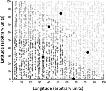
1) Random zones were generated within the fields. The method used to generate the random zones consisted in choosing randomly the centres of zones within the field. Then, each observation x i was affected to the nearest management zone centre, i.e. the centre with the minimum euclidean distance to x i (Fig. 1).
-
2) ANOVA tests (p<0.05) were conducted to evaluate if the management zones (randomly generated) were able to explain differences in AI values.
-
3) Steps 1) and 2) were run 1000 times (N=1000) for each field for a growing number of management zones.
-
4) The number Nt of occurrences for which the null hypothesis H0 is rejected with a probability p was computed for each iteration. The percentage of significant (Nt/N) results arising from the ANOVA tests was reported. For a large number N, it is expected that the Nt/N ratio tends to p (p being the probability of accepting H0 when at least two of the generated zones have a different mean).
Example of five random zones generated on a hypothetical field with Five centroids (black circles) randomly chosen inside the field to delineate the five management zones

Accounting for spatial autocorrelation by adjusting the sample size of the dataset
Dale and Fortin (2005) have proposed a clear and understandable review regarding how spatial autocorrelation have to be taken into account in statistical tests. This section focuses on some of their proposals for ANOVA tests. In the statistical tests concerning the mean of observations in absence of spatial autocorrelation, the variance of the mean is estimated as the sample variance divided by the sample size (Equation 1):
 $$var\left( {\bar{x}} \right)\,{\equals}\,s^{2} \!/n$$
In presence of spatial autocorrelation, the sample size n has to be re-evaluated because many observations account for the same spatial information. More precisely, this sample size has to be decreased to meet the requirement of independent observations for traditional statistical tests. In this case, the effective sample size becomes n', not n, and the variance is estimated as indicated in Eq. 2:
 $$var\left( {\bar{x}} \right)\,{\equals}\,s^{2} \!/n'$$
Cressie (Reference Cressie1991) have proposed another way to accommodate
 $var\left( {\bar{x}} \right)$
in case of spatial autocorrelation of the x’s (x
1
, x
2
, ….x
n
). This author has suggested to express
 $var\left( {\bar{x}} \right)$
with the covariances of the x’s, hereafter referred to as cor (x
i
,x
j
) . By substituting the formula of Cressie (Reference Cressie1991) with Eq. 2, the effective sample size (n’) can be estimated as follows:
 $$n{'} \,{\equals}\,{{n^{2} } \over {\sum_{i\,{\equals}\,1}^n \sum_{j\,{\equals}\,1}^n cor(x_{i} ,x_{j} )}}$$
Where n and n’ are respectively the sample size and the effective sample size, cor (x i ,x j ) is the correlation between observations x i and x j
When a semi-variogram model can be fitted relatively well to the observations, cor (x i ,x j ) can be deduced from the variogram model parameters. As an example, equation 4 shows how cor (x i ,x j ) is estimated when a semi-variogram is fitted with an exponential model:
 $$cor\left( {x_{i} ,x_{j} } \right)\,{\equals}\, {{C_{1} .e^{{({\minus}{{h_{{ij}} } \over a})}} } \over {C_{0} {\plus}C_{1} }}$$
Where h ij is the distance between observations x i and x j . The parameters a, C0, and C1 respectively stand for the range, the nugget effect and the partial sill retrieved from the exponential model.
One-way ANOVA aims at comparing the means of g groups (i.e. zones), with H0 stating that the mean is the same for all groups. One-way ANOVA involves the comparison of the ratio of equation 5 to the Fisher distribution. Here, in case of spatial autocorrelation, the sample size n is replaced by n’, the effective sample size (Eq. 5):
 $${{CSS_{{groups}} /\! \left( {g{\minus}1} \right)} \over {CSS_{{residual}} /\!\left( {n^{'} {\minus}g} \right) }}$$
Where CSS is the corrected sum of squares of means, and (g–1) and
 $(n{'} {\minus}\,g)$
are the corresponding number of degree of freedom.
This approach was used on a real dataset with spatially dense agronomic information (see data section) from which a semi-variogram was computed and fitted with a known variogram model. Management zones were defined with the auxiliary information of this dataset in two different ways, either randomly or following the auxiliary information. ANOVA outputs were reported by using Eq. 5 either by using the sample size n or the effective sample size n’.
Accounting for spatial autocorrelation by randomization methods
The previous method applies only when it is possible to fit a specific model to a semi-variogram derived from the data. In some cases, this might not be possible, e.g. when the number of observations is too small (n<40) or when a field exhibits non-stationary processes. In these cases, one possibility would be to use randomization methods (Dale and Fortin, Reference Dale and Fortin2002). These approaches aim at comparing a test statistic calculated from the original dataset with the distribution of the same statistic calculated after it has been randomized.
The Wilks index (λ), i.e. the ratio of the within zones variance over the total variance, is a widely used statistic to evaluate the performance of a zoning procedure. Here, the randomization consisted in a six step-process:
-
1) An expert delineation is performed (ZE), i.e. following the auxiliary information available (zones are not randomly drawn),
-
2) λ value is calculated for the previously generated zoning ZE (λE),
-
3) Random contiguous zones (ZR) are generated within the field,
-
4) λ value is calculated for the previously generated zoning ZR (λR),
-
5) Steps 3) and 4) are repeated a large number of times (N>1000), and
-
6) The distribution of all the λR values is computed. The zoning ZE may be considered significant (p<0.05) if the probability to observe λE is smaller than a threshold α (α is set to 5%) given the probability distribution of all the λR.
This approach was used on the same dataset as that for the methodology in 2.2 except that the number of agronomic information was significantly reduced. The objective was to have few observations so that it was not possible to derive a semi-variogram from the dataset.
Data sets
Real and simulated datasets were used to perform the tests:
-
∙ Hypothetical fields of known spatial variability were obtained from a simulated annealing procedure (Goovaerts, Reference Goovaerts1997). Parameters of the hypothetical fields have been chosen according to grape fields characteristics (Taylor et al., Reference Taylor, Tisseyre, Bramley, Reid and Stafford2005). For all the fields in our data-base, semi-variograms were fitted with an exponential model in which the nugget effect was approximately set to one third of the sill. For all the fields, it was decided to apply a nugget effect of 5 and a sill of 16 (arbitrary units). Fields only differed by the range of their semi-variogram. Three fields were simulated with practical ranges of 18, 27 and 36 m (respectively data_2, data_3 and data_4). Another field was simulated with no spatial structure, i.e. pure nugget effect (data_1). All the fields have an area of 1 ha (100×100 m) and a resolution of 2000 points/ha (Fig 1).
-
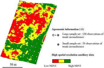
∙ Real data corresponds to a 1.4 ha vine field of variety Mourvedre located at the research vineyard of INRA at Domaine de Pech Rouge (Gruissan, Aude, France) (RGF93 datum, Lambert93 coordinates: E: 709 800, N: 6 226 840). Auxiliary information corresponds to NDVI values derived from a multispectral airborne image at 1 m resolution acquired at veraison (Fig. 2). The agronomic information (AI) corresponds to the trunk circumference measured on a 15×15 m grid size.
NDVI map with associated samples of trunk circumference. Two datasets were created from the trunk circumference samples to test the two proposed correction approaches.

Results and discussion
Impacts of AI spatial auto-correlation on the significativity of management zones
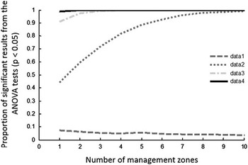
For dataset 1 which does not exhibit any spatial autocorrelation, ANOVA tests deliver conclusive results in approximately 5% of the cases (Fig. 3). This outcome is observed whatever the number of management zones that were put into place. This result should have been more or less obtained for all the datasets if the spatial autocorrelation had been taken into account given the randomly defined zones. However, as the spatial structure of AI information increases, i.e. from dataset 1 to dataset 4, ANOVA tests conclude very often that the management zones explain differences in AI values (in more than 50% of the tests). Even more surprising, when the spatial structure is strong enough (datasets 3 and 4), almost all the outputs of ANOVA tests are significant. Remind that the zones are defined completely randomly. In other words, when an AI variable exhibits a high spatial autocorrelation, regardless of the zoning considered, the ANOVA test will always conclude that the zones are significantly different from each other. Another interesting fact is that for dataset 2 and 3, the proportion of significant results from ANOVA tests increases with a growing number of management zones. It is even much easier to obtain significant results when lots of management zones are delineated. This plot confirms that the spatial correlation of AI information is a critical issue and should be carefully examined before validating the relevancy of an auxiliary variable to define management zones.
AI spatial structure and incidence on the significativity of ANOVA tests.

The simulated data are used here for demonstration and validation purposes. This validation was voluntarily carried out on a very large number of data. From a practical point of view, it is evident that in such a situation the use of auxiliary data with high spatial resolution is of no interest and that the zoning would be carried out directly on the data of interest. This high number of data also allows the consideration of a large number of management zones which may be not realistic on a real example. The next section aims at showing an application with a more realistic dataset from a real case where a small number of measurements are available.
Evaluating the two proposed approaches to overcome the AI spatial auto-correlation issue
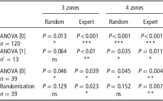
Table 1 reports the degree of significativity of the traditional ANOVA approaches and the corresponding proposed corrective methods. For large datasets of agronomic information (n>40), first method, ANOVA [1] is an interesting way to account for spatial autocorrelation. It is clear that the significativity of the ANOVA tests is more severely re-evaluated and it will prevent users from making bad management decisions. Indeed, all the p-values are much higher than for the traditional ANOVA approach, ANOVA [0]. In the case of expert-based management zones, both methods generate significant results. In this work, the objective was to evaluate if the NDVI was a good indicator of the temporally stable vigour variability (estimated with the trunk circumference) inside the field. Not surprisingly, results exhibit a good significativity because there is actually a well-assessed relationship between vine vigour and NDVI. However, when the relationship between the agronomic information and the auxiliary data is not clear enough, which has been represented by randomly-defined zones, traditional ANOVA methods can generate misleading conclusions. More precisely, when random zones are drawn inside the fields, the corrective method ANOVA [1] concludes to a relatively poor significativity, and even states that the three randomly-defined management zones do not explain the variability observed in the trunk circumference values. Note that the randomly-drawn zones do not prevent the traditional ANOVA approach to generate very significant results. It can also be observed that the p-values are lower for four than for three management zones which is consistent with the results found in Figure 3. Indeed, significant conclusions are more likely to be obtained as the number of management zones increases within the fields.
Significativity of the traditional and corrected ANOVA approaches. P-values are reported.

ns: non-significant results, * significant results (P<0.05), ** strong significativity (P<0.01), *** very strong significativity (P<0.001)
This first method is definitely a useful approach to better evaluate the significativity of ANOVA approaches. Moreover, the evaluation of the AI spatial structure is not dramatically complex when enough observations are available. However, two issues of the method need to be discussed. First of all, the method requires to model and to characterize the spatial structure of the AI information. Since the adjustment of the sample size relies on an accurate estimation of this spatial structure, a bad evaluation of the semi-variogram parameters might have an effect on the new sample size that is used. Secondly, it must be clear that this method can be applied if and only if the number of observations is large enough. Generally, relatively few AI observations are acquired within the field which makes the first method not largely usable.
For a small number of samples of agronomic information (n<40), the corrective approach, i.e. randomisation, also generate higher p-values than the traditional ANOVA approach ANOVA [0] (Table 1). Results are consistent with those observed for a large datasets of trunk circumferences, i.e. a relatively good significativity for expert-based management zones and non-significant results for randomly-based management zones. Results prove the usefulness of the randomisation approach which is able to severely penalise the randomly-defined zones; p-values are superior to 0.1 even for four management zones. This approach might be much more usable than the previous one, i.e. ANOVA [1], because it is likely that samples of agronomic information might not be widely available. When the randomisation method generates significant conclusions, it has to be understood that the zoning under study, the one that is evaluated, can be considered better than most of the possible zonings. It does not necessarily mean that the auxiliary data greatly explains the variability in the agronomic information. It can only be concluded that, among all the conceivable zonings, the proposed zoning is one of the most relevant.
Conclusion
The main objective of this paper was to warn the precision agriculture scientific community about the non-appropriate use of ANOVA tests when observations are spatially auto-correlated. Two methods were proposed to take into account this spatial correlation and to make the conclusions from ANOVA tests more reliable. Users should be very careful about the requirements of traditional (non-spatial) methods before applying it directly on spatial datasets. Indeed, most of the commonly used statistical tests require the observations to be independent from each other which is rarely the case in agronomic or environmental datasets. It is strongly recommended that future studies report and account for spatial autocorrelation not to misinterpret the outcomes of commonly used statistical tests.