


Introduction
The impact of the First Globalisation and the interwar period on the well-being of the Latin American population remains subject to debate.Footnote 1 In recent decades, the international comparison of living standards has relied primarily on real wages. This approach assumes that real wages serve as a better measure than aggregate variables such as gross domestic product (GDP) per worker or per capita for periods for which official statistical data are lacking.Footnote 2
According to Jeffrey G. Williamson and Timothy J. Hatton, the wave of international integration during the First Globalisation boom led to major shifts in relative prices, which, in theory, should have driven wage convergence – especially between Europe and the Americas, the so-called ‘Atlantic Economy’.Footnote 3 Other scholars (see notes 13–16 below) argue that alternative forces dominated, which helps explain why factor returns, such as wages, did not converge despite market integration. These other forces include differences in productivity growth and in institutional arrangements that impact productivity growth and distribution.
As for Latin America, Luis Bértola and colleagues explain variations across countries as well as divergence from the world’s leading economies along similar lines.Footnote 4 Pablo Astorga, who used as a basis a new series of real wages for six Latin American countries, assessed the influence of structural change dynamics and, in particular, how the terms of trade account for differences in real wages and skill premiums across countries and time periods.Footnote 5
We contribute to this debate by providing new estimates of comparable real wages. We calculated a new set of purchasing power parities (PPP) to adjust real wages for the capital cities of the Latin American Southern Cone: Buenos Aires, Montevideo, Santiago de Chile and Rio de Janeiro. We used London as the reference point since it was the leading economy during this period (1870–1939), although its global dominance began to decline in the interwar years.
Our approach follows the methodology initially proposed by Williamson and subsequently replicated by Bértola and colleagues.Footnote 6 The benchmark estimates were based on a consumption basket which includes food and housing as primary family expenditure items. For the food baskets, our estimate was based on the city’s specific diet while aiming to hold calorific intake constant.Footnote 7 For housing, we incorporated information on rental costs. Given the common practice of families renting rooms in types of collective housing in the Latin American cities under study, we presented two scenarios: an estimate based on the rent for a one-room dwelling unit and a second estimate based on the rent for a three-room unit. While we believe the one-room dwelling unit better characterised the conditions of working-class families, we retained the three-room dwelling unit for comparative purposes with previous studies and to provide an alternative measure to assess the sensitivity of our results to this decision.
Given that the primary data on wages, prices and household expenditure was available only for the capital cities, our analysis was restricted to these urban centres. Furthermore, the information predominantly related to the unskilled urban labour force, which Astorga estimated as constituting approximately 40 per cent of the labour force in Argentina and Chile and 70 per cent in Brazil.Footnote 8
Throughout the period under study, the countries experienced significant economic change, though with varying levels of performance both between and within them.Footnote 9 The First Globalisation was marked by intense flows of goods and capital into Latin America, along with significant migration movements. World War I disrupted the pace of economic change, and the 1920s witnessed a decade of rapid recovery. This progress came to an abrupt halt in the wake of the 1929 Crash, which triggered a profound economic shock that led to a decade of slow growth and depression. The 1930s were characterised by slow economic expansion and state-led industrialisation, with the latter persisting into the 1980s.
The countries that make up Latin America’s ‘Southern Cone’ – Argentina, Chile, Uruguay and Brazil – experienced substantial immigration during the period under study. The first three underwent stronger economic expansion – largely driven by these inflows, along with more dynamic labour markets – and enjoyed better living standards than Brazil.
The results offer new insights into living standards and real wages during the First Globalisation, revealing marked disparities across Southern Cone cities. In the early twentieth century, wages in the Río de la Plata capitals were close to London levels, while those in Rio de Janeiro were less than half as high, with Santiago in between. By the 1930s, all four capitals had seen a deterioration in their relative real wages. Comparing the two temporal scenarios emphasises the importance of using more than one benchmark to study this historical period. The body of evidence presented is consistent with previous studies that cast doubt on the validity of the convergence hypothesis for the western side of the Atlantic. In terms of trajectories, the real wages adjusted by PPP in the Southern Cone illustrate a pattern of divergence over the entire period compared to London levels. Montevideo failed to maintain its initial standards, while real wages in Buenos Aires displayed an inverted U-shape, converging until the late nineteenth century before changing direction. Rio de Janeiro shared similar movements with Buenos Aires but at a considerably lower wage range, while Santiago de Chile exhibited a divergent pattern that intensified in the twentieth century.
The rest of the paper is organised as follows. The next section provides brief historical context. We then discuss methodology and data sources, then the results of the PPP estimates and the adjusted real wages, offering a comparative analysis of living standards between the Southern Cone cities. Finally, we draw our conclusions and outline the next steps in the research agenda. The article includes an online Appendix (URL provided at the end of this article) with detailed information about the sources and the data used to estimate the PPP converters for adjusted real wages in each city.
The First Globalisation, the Interwar Period and the Convergence Hypothesis
The period under study spans the First Globalisation and the interwar period. By the late nineteenth century, Latin America was fully integrated into global trade as a net exporter of raw materials and a net importer of manufactured goods, within a new international economic order primarily dominated by Great Britain and based on free trade. The First Globalisation was characterised by an intense flow of goods and capital into Latin America, along with massive migration movements. During these decades, the countries of the Southern Cone experienced significant economic change, primarily driven by exports (which were mostly concentrated in primary products), although there was considerable heterogeneity in performance between and within countries.Footnote 10
Williamson and Hatton argue that, during the peak of the First Globalisation, global economic integration altered relative prices in ways that should have encouraged wage convergence, notably among Atlantic Economy countries.Footnote 11 This convergence was also attributed in large part to the intense mobility of the population between Europe and the countries across the Atlantic during these decades. Latin America received approximately 12 million European and Asian immigrants (one-fifth of global emigration). Most of this contingent arrived in the post-World War I period, with Southern Cone countries being the main recipients: Argentina, Brazil, Chile and Uruguay.
According to Williamson, there were two phases: a rapid convergence of factor prices between 1870 and World War I, followed by a period of regression in the interwar period. Between 1870 and World War I, in a context of free trade, capital flows and massive migrations, there was a convergence in the relative prices of factors, both among peripheral countries and between these countries and Europe.Footnote 12 However, other perspectives argue that there was no convergence in factor prices, despite market integration, due to the influence of other elements, such as differences in productivity growth, productive structures, technological capabilities, market structures (labour and land), geography and institutional arrangements impacting growth and distribution.Footnote 13 Robert C. Allen, for example, showed that there was no convergence at all between the English-speaking countries in the period 1879–1913.Footnote 14 David Greasley, Jakob B. Madsen and Les Oxley relate real wage differences to divergent patterns of industrial organisation and productivity growth in Australia and New Zealand as compared with the United States and Canada.Footnote 15 Other studies question the pace of convergence.Footnote 16
Regarding the Latin American experience, Bértola and his collaborators find that both convergence and divergence regimes existed, depending on the decades and countries under scrutiny.Footnote 17 The relationship between openness and convergence is not as straightforward as predicted by the theory. Bértola, María Camou and Gabriel Porcile cite the case of Argentina between 1870 and 1900 as a good example:Footnote 18 while massive migration during these decades should have depressed real wages in receiving countries and increased them in sending countries, Argentina did not converge with the leading countries. Another aspect highlighted by these authors is that Argentina and Uruguay had lower wages than north America, but both countries received large migration inflows in the late nineteenth and early twentieth centuries. The authors argue that real wages in Latin America faced constraints derived from the distribution of land and income in rural areas. They conclude that the long-term evolution of wages depended on productivity and, therefore, other aspects must be included in the analysis, such as land ownership, the labour market, the formation of the national state, and the relationship of economic productivity to technological change, income distribution and education.
In a later work, Bértola and Ocampo claim that performance varied between Latin American countries during the First Globalisation.Footnote 19 Although it was a period of overall improvement in real wages, significant divergence persisted. Real wages increased in all the countries that they sampled (Colombia, Brazil, Cuba, Argentina, Chile and Uruguay) at least until 1910. Mexico appears as an exception, with stable levels until the post-revolution period, followed by a decline in real wages. Colombia experienced a lagged expansion of real wages that seemed to align with its economic progress. This diversity of trajectories challenges Williamson’s hypothesis about the positive impact of the First Globalisation on factor prices, as it fails to explain the divergent patterns across countries.Footnote 20 Brazilian, Colombian and even Chilean wage levels remained far from those reached by the developed economies. Bértola and Ocampo explain Latin America’s lagging performance by pointing to a range of factors, including labour market structures and regulation, the segmented nature of international migration (with European migrants concentrated in new settlement economies and Asian populations in tropical regions), differences in productivity levels, the specific ways in which productivity gains were appropriated, and the role of rents derived from natural resource exploitation.Footnote 21
This brief overview shows that the discussion of the effects of the First Globalisation on factor prices, especially on real wages, remains open to debate and, above all, to the presentation of new evidence.
Methodology
There are two main challenges to address when comparing real wages across countries: first, determining which wage is more suitable for comparison; and, second, determining how to measure the purchasing power of this wage in comparative terms to control for different prices over time and between countries. To address the former challenge, some authors have used as a reference the wage of an unskilled labourer in the building industry.Footnote 22 For the latter challenge, one solution is to construct converters such as PPPs with which to adjust nominal wages. Such a procedure is necessary because the exchange rate may not correctly indicate the differences in prices between two countries, especially if non-traded goods and services are included.Footnote 23 Diverse procedures have been used to adjust real wages to internationally comparable units for historical periods. For example, some authors propose calculating PPP benchmarks for comparable consumption baskets suitable for adjusting real wages.Footnote 24 Other studies provide welfare ratios based on the purchasing power of nominal wages with respect to a standardised subsistence consumption basket.Footnote 25
In this paper, we employ the former method and construct PPPs. As in previous studies, London is taken as the reference.Footnote 26 The benchmark estimates are based on a consumption basket, which includes food and housing, the primary family expenditure items. These baskets are designed to be equivalent in terms of calorific intake, and the composition varies between countries depending on local preferences and habits. Regarding the housing component, these baskets include direct rental cost information for a one- and a three-room dwelling.
The PPP coefficients were obtained by comparing the prices of goods in two cities: one from our Latin American sample – Buenos Aires, Rio de Janeiro, Santiago de Chile or Montevideo – and London.Footnote 27 These prices, expressed in their respective national currencies, were weighted according to their significance in consumer expenditures. To determine the weights for food and rent, we used the geometric mean of the expenditure shares for these categories in the two cities. The overall PPP was then computed as a weighted sum of the PPPs for these two expenditure categories.
We constructed the PPP indices for two points in time: 1905, as representative of the period 1870–1913, and 1938, representing the post-export-led period (1914–40).Footnote 28 The selection of these years was mostly based on the availability of information. The first benchmark corresponds to the peak or near-peak of globalisation, while the second benchmark corresponds to the end of the backlash against globalisation. While the most common classification used in the developed world considers the 1920s as being part of the interwar years, for Latin America the most frequently used classification extends the globalisation period until the economic crash of 1929.
Nevertheless, as Rosemary Thorp, and Bértola and Ocampo, have pointed out, the export-led era came to an end at different times in different countries:Footnote 29 in Argentina and Uruguay, there seem to have been contrasting shifts in the globalisation trend following the economic crises of World War I.
In the following sections, we describe the information and methods used to estimate the primary expenditure components: food baskets and housing.
Food Baskets
We constructed nutritionally equivalent consumption baskets on the premise that individuals can obtain similar levels of metabolic energy from different combinations of macronutrients – carbohydrates, proteins, and fats.Footnote 30 We allowed for variations in components between cities due to geographical conditions and consumption habits, while ensuring that all baskets provided the same calorific intake.
Food baskets were designed based on the following assumptions. First, we considered a family composition of two adults – one male and one female – and two children. The assumption of a four-member family was based on sources from Montevideo. However, household size might have varied in other cities. Despite these variations, assuming two adults and two children is commonly used for international comparisons; for instance, Allen employed this household size.Footnote 31 Second, we assumed that the household food basket supplied 8,023 kcal/day. This assumption is based on the reference value of 2,850 kcal/day, the recommended energy requirement for an adult male aged between 18 and 30, with an average height ranging between 1.60 and 1.75 m and an average weight between 65 and 70 kg.Footnote 32 To establish the consumption per equivalent adult, we employed adult-equivalent conversion factors for estimated calorific requirements based on age and gender, as computed by Jane Humphries and adapted to the data reported by the FAO.Footnote 33 The adult-equivalent fraction assigned to each member of the family was calculated as the ratio of calorific requirements (by age and gender) to the estimated adult reference value of 2,850 kcal/day. Using these conversion factors, the daily calorific requirements were 2,375 kcal/day for women and 1,399 kcal/day for children under ten years of age. The total daily calorific intake for a family of four members, amounting to 8,023 kcal/day, resulted from the sum of 2,850, 2,375 and (1,399 x 2).
To measure the representativeness of the assumption regarding total household calorific intake, we contrasted it with additional data from Montevideo and London. These two cities provided historical sources on household food consumption for this period. The budget for Montevideo reflected the commodities consumed by a working-class family of two adults and two children under 14 over one week during 1914.Footnote 34 Meanwhile, the British budget was based on the quantities of selected commodities consumed by a working-class family consisting of two adults and three or four children over one week during 1904 in London.Footnote 35 To compare the calorific intake of households with different compositions, we converted per capita calorie consumption into consumption per adult male equivalent. After these adjustments, we calculated that the food basket for Montevideo provided 3,687 kcal/day per adult-equivalent. In London, the calorie intake per adult-equivalent ranged from 2,890 to 3,319 kcal/day, depending on whether the family included three or four children. Thus, our assumption of 2,850 kcal/day closely aligned with the scenario of a London family with four children and represented slightly more than two-thirds of the calories consumed by a family in Montevideo in 1914.
Our basket reflected societies that had moved beyond subsistence income levels and had entered a more advanced stage of the nutrition transition. According to David Grigg’s conceptual framework, these societies were highly modern in terms of nutrition, with a daily intake ranging from 2,300 to 3,200 kcal and a significant proportion of their diet derived from animal products (meat, dairy).Footnote 36 Compared to the bare-bones subsistence basket for a family of two adults and two children calculated by Allen, our basket is substantially richer, incorporating a wider variety of foods and providing, on average, roughly twice as many calories. Allen’s basket, which yields only 1,941 kcal per adult-equivalent per day, was designed as a ‘poverty line’ to construct a long-run price index for Europe dating back to the Middle Ages and, as he notes, resembles a pre-modern consumption pattern.Footnote 37 In terms of total intake, our basket is more similar to Allen’s ‘European respectability basket’, which provides 2,500 calories per day for an adult.Footnote 38
Once we had defined the number of calories the basket should yield, the composition of each basket varied between cities depending on local food habits. To construct the equivalent household consumption basket that yielded 8,023 kcal/day for each city, we proceeded differently, depending on the type of available data sources.
For London, the data were based on a selected basket representing the quantity of foodstuffs assumed to be consumed weekly by a working-class family of two adults and two children in 1904.Footnote 39 For Montevideo, we used the quantities of food consumed by a working-class family of two adults and two children in 1914.Footnote 40 Adjustments were made to the original quantities of key food items to meet the target of 8,023 kcal/day. Following the report by the Ministerio de Industrias y Trabajo (Ministry of Industry and Employment) of an inquiry into working-class families in Montevideo in 1937, we reduced the annual household consumption of beef from 547 to 420 kg and of milk from 547 to 360 l.Footnote 41
For the other three cities – Buenos Aires, Santiago de Chile and Rio de Janeiro – we could not find complete information about the quantities of food consumed by a working-class family around the beginning of the twentieth century. Therefore, we used several sources and assumptions to construct equivalent food baskets.
For Buenos Aires, we initially considered that the diet consisted primarily of meat, bread, milk, oil, rice, sugar, coffee, yerba mate, flour, potatoes and lard, as indicated by various studies.Footnote 42 Second, we ascertained the quantities consumed. The Boletín del Departamento Nacional del Trabajo (National Labour Bulletin, Boletín del DNT) reported on the food consumption of a working family with four members. We used the annual quantities of milk (420 l) and adjusted the quantities of bread (420 kg) and meat (420 kg) to match the equivalent calorific intake.Footnote 43 Two additional considerations were: firstly, the quantity of meat consumed was the same as the quantity of bread, according to Roberto Cortés Conde;Footnote 44 secondly, the distribution of total meat consumption (420 kg) between beef, mutton and pork corresponded to the percentages described as typical by Alejandro Bunge: 80 per cent beef (336 kg), 15 per cent mutton (63 kg) and 5 per cent pork (21 kg).Footnote 45 The quantities of sugar, potatoes, rice and wheat flour were calculated from information provided by Juan Alsina.Footnote 46 Based on the per capita monthly quantities consumed, we calculated the amount needed for a family of four members using the conversion factors discussed above.Footnote 47 Finally, to complete the basket, we needed to include maize flour, lard and yerba mate, so we assumed the same amounts of these foodstuffs as in Montevideo, given that Buenos Aires and Montevideo at that time shared a similar culture regarding food habits, due to similar natural endowments and immigrant influences.Footnote 48
The equivalent food basket for Rio de Janeiro was based on the studies of Eulália Maria Lahmeyer Lobo and colleagues, and of Léo de Affonseca Junior.Footnote 49 Lobo studied several features of the working classes in Rio de Janeiro, with a special focus on salaries and the cost of living.Footnote 50 Based on food studies for Rio de Janeiro, she selected the most important foods in the diet of the working-class: rice, beans (feijão), dried meat (charqui), cassava flour, sugar, cod (bacalhau), bacon, coffee, wheat flour, butter and beef.Footnote 51 For the first eight items, she presented the monthly food consumption of the typical worker in Rio de Janeiro in 1892.Footnote 52 We calculated the annual calories per capita of each type of food and converted them to the equivalent consumption of an adult couple and two children using the male adult equivalent conversion factor.Footnote 53 Finally, we calculated the annual implicit quantities that yielded these volumes of calories. For the quantities of the last three items – wheat flour, butter and beef – we referred to Affonseca,Footnote 54 Director of Commercial Statistics at Brazil’s Ministry of Finance, who presented a consumption basket for a family of seven members in Rio de Janeiro and reported on the prices of the items in 1893, 1914 and 1919. Affonseca’s study did not provide detailed demographic information about the family in question, but – as noted by Lobo et al. – their pattern of consumption was likely characteristic of a middle- or upper-income household, as it included expenditures on servants.Footnote 55 We followed the same procedure as before, that is, first calculating the calories of each food item and then adjusting the quantities according to the amount needed to satisfy the nutritional needs of a family of two adults and two children.
Finally, for Santiago de Chile, we based our analysis on the equivalent consumption baskets described by Jorge Errázuriz Tagle and Guillermo Eyzaguirre Rouse, and Juan Carlos Yáñez Andrade.Footnote 56 Errázuriz and Eyzaguirre detailed the living conditions of a working-class family in Santiago de Chile in 1902 and reported on the consumption habits of a household comprising three adults and six children.Footnote 57 From this study, we derived the quantities of sugar, lard, potatoes, maize flour, bread, mutton, eggs, beans, rice and noodles.Footnote 58 The consumption of milk and beef was based on references in Yáñez Andrade to a medical study on the nutritional conditions of working families in Santiago de Chile in 1935, which included daily calorific intake.Footnote 59 We calculated implicit quantities and adjusted the daily consumption of milk and beef to meet the requirements of a family of two adults and two children, which forms the basis of our analysis. Finally, for tea (7 kg) and coffee (7 kg), we adopted British annual tea consumption (14 kg) and shared it between the two beverages.Footnote 60
Table 1 displays the commodities and final quantity estimates for each food basket, while Table 2 reports for each city the total estimated annual intake of calories, proteins and fats.
Equivalent consumption baskets around the beginning of the twentieth century in five cities: Annual household consumption

Table 1 Long description
The table compares annual household consumption of various food items in five cities around the early 20th century. London shows the highest consumption of wheat flour and bread, with 172 kg and 378 kg respectively. Buenos Aires and Montevideo have significant milk consumption at 420 liters each, and high beef intake, with Buenos Aires at 336 kg and Montevideo at 360 kg. Rio de Janeiro stands out for its high consumption of rice and cassava flour, at 51 kg and 86 kg respectively. Santiago de Chile has notable bread consumption at 369 kg. The data highlights regional dietary preferences, with some cities lacking data for certain items, indicating possible differences in availability or cultural preferences.
Household = four-person family comprising two adults and two children
Equivalent consumption baskets around the beginning of the twentieth century in five cities: Annual household consumption of total calories and macronutrients

Table 2 Long description
The table compares annual household consumption of calories, proteins, and fats in five cities around the early 20th century. Montevideo leads in protein and fat consumption, with 174,391 kg of proteins and 165,691 kg of fats. London has the lowest protein intake at 94,042 kg, while Santiago de Chile has the lowest fat consumption at 42,511 kg. Caloric intake is relatively similar across all cities, with Buenos Aires having the highest at 2,972,430 kcals and Santiago de Chile the lowest at 2,862,629 kcals. The data suggests significant variation in macronutrient consumption, particularly in proteins and fats, which may reflect dietary preferences or availability in these regions during that period.
Household = four-person family comprising two adults and two children
Housing
We calculated housing costs for two different housing scenarios: the rent for a one-room and for a three-room dwelling. Williamson and Bértola et al. used the latter rate, which reflects the rental situation typically described for British working-class households during the period in question;Footnote 61 this assumption does not apply to working-class households in the Southern Cone cities during this period. From the end of the nineteenth century, and especially during the first decades of the twentieth century, the working classes in major Latin American cities faced a housing shortage.Footnote 62 Housing supply failed to keep up with the increased demand resulting from rapid urbanisation and the dramatic growth in migration flows. Rent was expensive in the urban areas, and families lived in overcrowded conditions. It was common for working-class households at that time to inhabit a single room, either in tenement houses (known as conventillos in Buenos Aires, Montevideo and Santiago de Chile, or cortiços in Rio de Janeiro) or in other types of dwellings. To control for the possibility that the choice of the English standard could distort differences in the estimated PPP real wage, we estimated a basket that would better reflect the Southern Cone housing case. As there was no principled reason to prefer one measure to the other, it seemed reasonable to consider both cases and assess whether the choice of housing scenario yielded differences in the resulting comparative living standard estimates. Below we explain some general features of housing conditions in the cities and the information used to calculate each benchmark and type of rent. See the Appendix for the sources and procedures.
Results: Living Standards in the Capital Cities of the Southern Cone
Once we had the equivalent food consumption baskets, we computed the weekly cost of each basket, added the cost of rent (for one room and for three rooms) and, thus, obtained the weekly consumption cost for each city, expressed in each nation’s currency. The weekly consumption cost was calculated for 1905 and 1938.
A Comparison of the Cost of Living
To compare the cost of living, the difference between the price levels can be represented by the price level index (PLI), a simple ratio of the PPP and the market exchange rate of national currency with respect to the British pound.Footnote 63 This ratio is expressed as an index with a base of 100. A PLI of 100 indicates that price levels are the same as those in the base city, while a PLI over 100 means that, when the national average prices are converted at prevailing exchange rates, the resulting domestic prices tend to be higher, on average, than prices in the base city. Table 3 provides the PLI for food and rent (one room and three rooms). In all cases, the indices take London as the base.
Price Level Index (PLI): Food prices and rent (one room and three rooms)

Table 3 Long description
The table compares the Price Level Index (PLI) for food prices and rent in one-room and three-room accommodations across four cities at two benchmarks: London 1905 and London 1938. In 1905, Rio de Janeiro had the highest food price index at 172, while Santiago de Chile had the lowest at 84. For rent in 1905, Buenos Aires had the highest index for one room at 179, and Rio de Janeiro had the highest for three rooms at 263. By 1938, Buenos Aires had the highest rent index for three rooms at 156, while Santiago de Chile had the lowest rent index for both one room and three rooms at 13 and 28, respectively. The data suggests a general decrease in food price indices from 1905 to 1938, with varying trends in rent indices across the cities.
Overall, relative prices in the four cities were higher in the pre-World War I period than in the 1930s. According to Table 3, food prices in the Southern Cone cities were generally equal to or lower than prices in London in both periods, with the only exception being Rio de Janeiro, whose prices were much higher during the earlier, turn-of-the-century period.Footnote 64
The comparison between the rent for one room and for three rooms deserves a more detailed discussion. As explained above, in London working-class families commonly rented three-room dwellings. Working-class families in the Southern Cone, however, typically rented one room. The rent for three rooms is relatively higher – almost double – than the rent for one room. It may be more appropriate, therefore, to compare the cost of intermediate-sized dwellings, e.g. two rooms. Nonetheless, if we compare the rent for a three-room dwelling, rent was much more expensive in Latin America, more than twice as high in Buenos Aires and Rio de Janeiro than in London. Santiago de Chile in 1938 is the lone exception, with a lower level. The differences in the rental price for one-room dwellings show that the cost of housing was lower in Latin America than in London, except for Buenos Aires and Rio de Janeiro, during the first decade of the twentieth century.
Another interesting finding is that housing in Latin America seems to have been more expensive at the turn of the twentieth century than during the interwar period. Previous studies have suggested some possible explanations for this result. Bértola et al. explain that mass immigration to the Southern Cone countries and the expansion of urban activities during the first decades of the twentieth century created substantial pressure on urban housing.Footnote 65 Other authors have discussed the impact of transportation costs on workers’ decisions to live near their place of work and how this contributed to rising housing rents (see the case of Montevideo described by José Pedro Barrán and Benjamín Nahúm).Footnote 66 Finally, higher rents may be explained by increased property values resulting from the fact that property constituted an important investment option in the absence of capital markets, at least in Rio de Janeiro.Footnote 67 This context of very high rents changed somewhat in the late 1930s. The combined effect of reduced European migration and an increased supply of affordable housing may have contributed to a decline in urban rents.Footnote 68 In Chile, the state enacted the Ley de Habitaciones Obreras (Workers’ Housing Law) in 1906, and the Decreto-Ley de Habitaciones Baratas (Affordable Lodgings Law) and the Decreto-Ley sobre Alquileres de Habitaciones (Renting of Lodgings Law) in 1925, in an effort to address the shortage in housing for the working-class population.Footnote 69 In Uruguay, the Instituto Nacional de Vivienda Económicas (National Institute for Economic Housing) was established by law in 1937 and several state initiatives addressing the shortage of affordable housing were implemented.Footnote 70 Similarly, in 1915, Argentina created the Comisión Nacional de Casas Baratas (National Commission for Affordable Housing).Footnote 71 (In the case of Brazil, state action in housing policy remained limited until the 1940s; the creation of the Fundação da Casa Popular (Foundation for Popular Housing) in 1946 marked a more explicit – though constrained – form of government intervention.)Footnote 72
A comprehensive overview of the cost of living can be obtained by comparing PPP estimates with nominal exchange rates and PLIs, as presented in Table 4.
Price Level Index (PLI): Purchasing Power Parities (PPPs) and Exchange rates (E)

Table 4 Long description
The table compares purchasing power parities (PPP) and exchange rates for one and three-room accommodations in four cities during two historical benchmarks: London 1905 and London 1938. Key data points show that Santiago de Chile had the highest PPP for one room in 1938 at 70.5, while Montevideo had the lowest at 5.2. Comparatively, Rio de Janeiro's PPP for one room increased significantly from 23.8 in 1905 to 45.5 in 1938. The price level index (PLI) for one-room PPP divided by exchange rate reveals that Buenos Aires had a notable decrease from 127 in 1907 to 74 in 1938. These figures suggest varying economic conditions and purchasing power across cities and time periods, with Santiago de Chile showing a marked increase in PPP by 1938. Interpretation should consider historical economic contexts and currency fluctuations.
From Table 4, we can highlight two results. First, the comparison of the two housing PPP coefficients reveals that the three-room rate gives a higher coefficient than the one-room rate, for all the cities and periods. Second, during the first benchmark period, the cost of living is higher than after World War I. If we focus on the first benchmark (1905), the cost of living closely approximated or exceeded (Buenos Aires, Rio de Janeiro and Montevideo) that in London (Table 4, columns 4 and 5). We find a different situation for Santiago de Chile, where the cost of living was between 9 per cent and 18 per cent lower than in London. The scenario changed by the late 1930s. The relative cost of living in the Southern Cone decreased relative to London; and Santiago remained the cheapest of the four capital cities. The differences obtained between the PPPs and the prices calculated using exchange rates (see Table 4) suggest that biased results can be obtained if nominal exchange rates are used to compare prices and wages, thus indicating the importance of obtaining PPP estimates.
Comparing the new set of PPPs to those estimated by previous authors yields another interesting result (Table 5).Footnote 73 It is important to remember that we are using a different food basket from those used by these previous authors, as well as different sources and prices for rent and, in some cases, other reference years. These factors may account, in part, for the differences in PPP. For the first benchmark, our PPP estimates are lower than in previous studies, with the only exception being Buenos Aires for the three-room scenario. Focusing on the results for the second benchmark, our new estimates of PPP are higher than those proposed by the other authors, regardless of the housing scenario used.
Previous estimates of Purchasing Power Parity (PPP) (based on three-room rate)

Table 5 Long description
The table compares historical purchasing power parity estimates for Buenos Aires, Rio de Janeiro, and Montevideo using two reference points: London in 1905 and 1927. In 1914, Buenos Aires had a purchasing power parity of 16.9 according to Bértola et al., while Rio de Janeiro in 1892 had a significantly higher value of 61.0. Montevideo's purchasing power parity in 1914 was notably lower at 7.3. For the year 1938, Buenos Aires had a purchasing power parity of 11.2, and Rio de Janeiro had a value of 42.3 according to Williamson's estimates, with Montevideo in 1927 having a value of 5.0. The data suggests that Rio de Janeiro had a relatively higher purchasing power compared to Buenos Aires and Montevideo during the periods measured. However, the absence of some data points indicates potential gaps in historical records or differences in estimation methods between the sources.
a Bértola, Camou and Porcile, ‘Comparación internacional’.
b Williamson, ‘The Evolution of Global Labor Markets’.
In general, we find relative prices in Latin America during the pre-World War I period were higher than in the 1930s, and this result may be explained by housing costs that appear to be, compared to London, more expensive at the turn of the twentieth century than during the interwar period. Buenos Aires and Rio de Janeiro are the most expensive cities, relative to London, during the beginning of the twentieth century. Santiago de Chile shows the lowest relative prices. Montevideo’s prices occupy the middle range. Finally, our new set of PPPs differs from previous findings for both one-room and three-room housing scenarios.
A Comparison of PPP-Adjusted Real Wages
Having discussed the main findings of the new set of PPP estimates, we now turn to the calculation of PPP-adjusted real wages. For the international comparison, we use wages for male unskilled labour in the urban construction sector. In a very few instances – such as for Chile in 1902 – we use instead the wage of another occupation with similar qualifications. Where possible, we used the wage per hour to avoid having to determine the average number of working hours.
Table 6 presents the new set of PPP-adjusted real wages relative to the wage in London in 1905 and 1938, for both the one-room and the three-room housing scenarios. A general result is that the real wages in all four Southern Cone cities are lower than in London (the only exception is Montevideo in 1905, when the PPP is calculated with the rent of the one-room housing scenario).
Purchasing Power Parity (PPP)-adjusted unskilled real wages relative to London in 1905 and 1938

Table 6 Long description
The table compares PPP-adjusted unskilled real wages in four cities relative to London in 1905 and 1938. Montevideo had the highest relative wages in both years, with 102.8 in 1905 and 82.7 in 1938. Buenos Aires followed, with wages decreasing from 86.0 in 1905 to 71.7 in 1938. Santiago de Chile's wages dropped significantly from 72.0 in 1905 to 32.4 in 1938. Rio de Janeiro consistently had the lowest wages, decreasing from 45.6 in 1905 to 35.2 in 1938. The data suggests a general decline in relative wages over time, with the most significant drop observed in Santiago de Chile.
PPP based on the one-room rent; London 1905 = 100.
We will focus our discussion of the difference in living standards based on the one-room housing scenario, as it better describes the conditions of the working classes in the south of Latin America during the period in question. Buenos Aires and Montevideo had higher real wages than did Santiago de Chile and Rio de Janeiro. Real wages in Santiago de Chile were higher than in Rio de Janeiro at the beginning of the twentieth century. However, the two cities switched positions during the 1930s, with real wages in Rio rising slightly above those in Santiago.
Based on the 1905 benchmark, real wages in Montevideo were very close to those in London and were higher than in Buenos Aires. In Santiago de Chile, we observe that the levels were almost as high as in Buenos Aires during the first benchmark period but much lower in the later period. According to Mario Matus,Footnote 74 between 1898 and 1902 real wages in Chile reached their peak during the economic expansion driven by saltpetre exports.Footnote 75 Thereafter, inflation eroded this positive trend and reduced all real incomes. This fact may explain the relatively high wage level indicated for 1902. In Rio de Janeiro, real wages remained comparatively low, in the range of 35–45 per cent of British real wages for both benchmarks.
This result is consistent with what the literature has generally reported based on real wages and on other well-being indicators.Footnote 76 Argentina and Uruguay had the highest level of economic growth of the four nations under study here, led not only by the export sector but also by the expansion of urban activities, the diversification of the economy with an early manufacturing industry and the development of infrastructure, communications, transport and financial services. These countries also achieved significant progress during this period on indicators such as life expectancy at birth, literacy levels, years of education and human capital. Chile performed like Uruguay, with very dynamic economic growth from the late nineteenth century, but with lower living standards as measured both by real wages and by performance on human development indicators. Brazil, by contrast, had the lowest per capita income level, consistent with its lower living standards on all the indicators mentioned above.Footnote 77
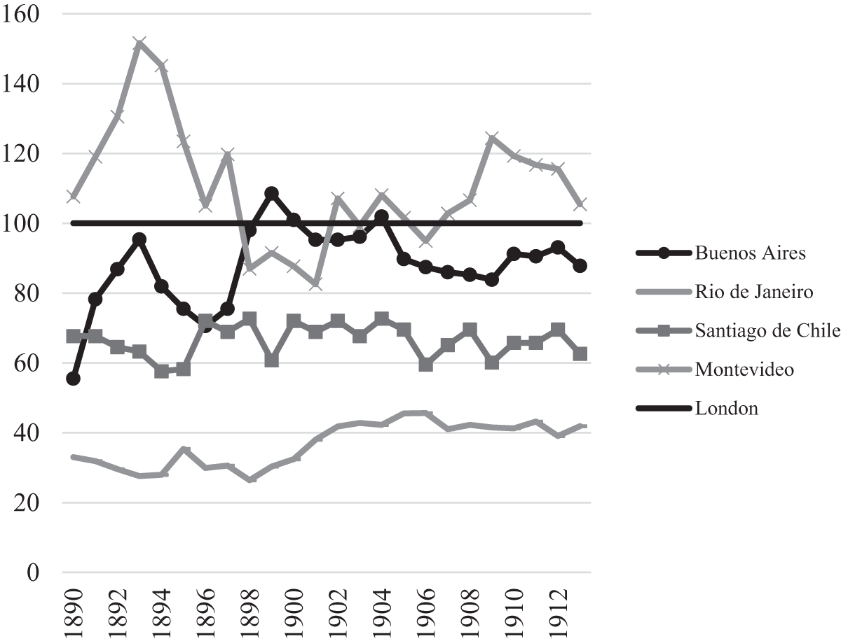
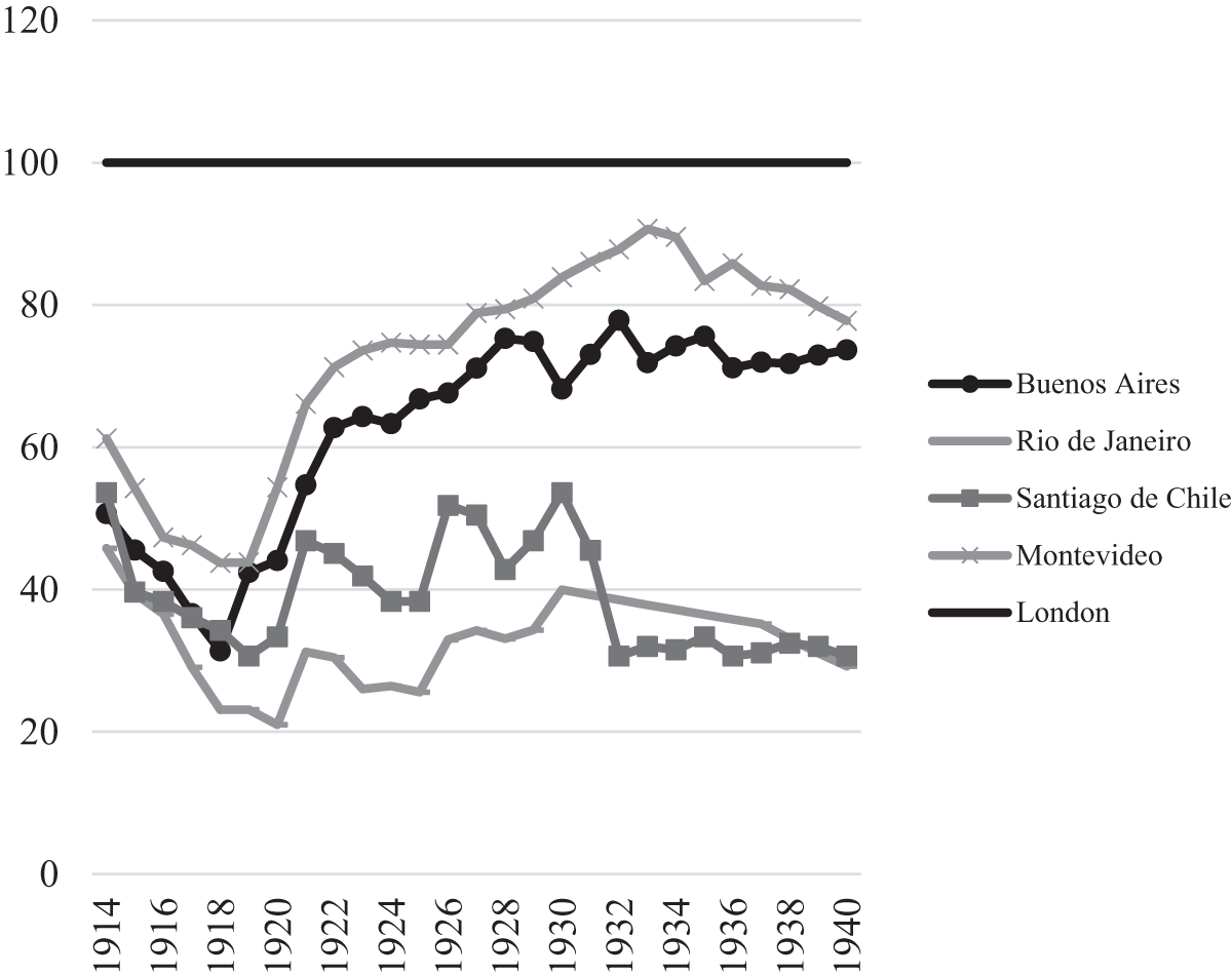
Figure 1 illustrates the series of PPP-adjusted real wages between 1890 and 1913 (with 1905 as the reference year), while Figure 2 shows the evolution of wages for the period 1913–40 (with 1938 as the reference year). The diverse trajectories in the different cities are evident. Montevideo fluctuates around London levels. Buenos Aires converges with London towards the end of the nineteenth century, but this trend seems to reverse later. The real wage in Santiago de Chile seems to oscillate around 67 per cent of the British salary, on average, throughout these years. Finally, in Rio de Janeiro, relative real wages doubled between 1890 and 1913, although they remained at very low levels in comparative terms, barely exceeding 40 per cent of the London wage.
Purchasing Power Parity (PPP)-adjusted real wages compared to London, 1890–1913 (1905 = 100)

Figure 1 Long description
A line graph showing Purchasing Power Parity-adjusted real wages from 1890 to 1912, with 1905 as the reference year. The x-axis represents years from 1890 to 1912 and the y-axis shows wage levels. Five lines represent different cities: Buenos Aires, Rio de Janeiro, Santiago de Chile, Montevideo and London. Buenos Aires fluctuates around the 100 mark, Rio de Janeiro starts below 40 and rises steadily, Santiago de Chile remains around 60, Montevideo peaks above 140 before stabilizing around 100 and London is represented by a constant line at 100. Each city is marked with distinct symbols for clarity.
Purchasing Power Parity (PPP)-adjusted real wages compared to London, 1914–40 (1938 = 100)

Figure 2 Long description
A line graph showing Purchasing Power Parity-adjusted real wages from 1914 to 1940. The x-axis represents years from 1914 to 1940, while the y-axis shows wage levels with 1938 as the reference year. Five lines represent different cities: Buenos Aires, Rio de Janeiro, Santiago de Chile, Montevideo and London. London is depicted as a constant line at 100. Buenos Aires starts below 40, rises to around 80 by 1940. Rio de Janeiro begins below 20, peaks near 60 in the 1920s, then declines. Santiago de Chile fluctuates around 40. Montevideo starts near 60, peaks above 80, then stabilizes around 60. The graph illustrates wage trends relative to London over the period.
After the phase of export-led growth, a relative deterioration in the living standards of South American cities in relation to London is observed, as all real wages declined. World War I negatively affected the relative wages of the four Latin American cities, and their subsequent trajectories diverge. On the one hand, Buenos Aires recovered and exceeded its starting levels, positioning itself as the city with the second highest wages after Montevideo, whose evolution was quite similar. On the other hand, Santiago de Chile showed a gradual deterioration, falling below Rio, which always remained below 40 per cent of British wages.
Overall, the years before World War I proved more prosperous for Latin American cities than the period after the export era, during which real wages fell well below those in London. World War I, the financial crisis of 1929 and the Great Depression changed the world economy, with significant effects on material standards of living. Relative prices changed dramatically, as shown above (Table 4). Therefore, using only one benchmark for the entire period can be misleading. Our argument is that, when analysing periods with significant changes in relative prices, it is essential to calculate convertors for each sub-period. By doing so, we can provide a more precise interpretation of the international comparison. For example, Figure 3 shows our analysis using the 1905 benchmark for the period 1890–1940 and, alternatively, 1938 as the benchmark. Although the evolution of each series is the same regardless of the benchmark adopted, in terms of living standards in Latin American cities in relation to London the results lead us to other conclusions. In particular, the image of the evolution of living standards in Buenos Aires and Montevideo is too optimistic when using the 1905 benchmark for the entire period and too pessimistic when using the 1938 benchmark. Overall, we observed an increase in the divergence of living standards among the cities.
Purchasing Power Parity (PPP)-adjusted real wages compared to London, 1890–1940: a) 1905 = 100; b) 1938 = 100

Figure 3 Long description
The first graph labeled 'a) 1905=100' shows real wages in Buenos Aires, Rio de Janeiro, Santiago de Chile, Montevideo and London from 1890 to 1938, using 1905 as the benchmark. The x-axis represents years from 1890 to 1938, while the y-axis shows wage index values ranging from 0 to 160. Buenos Aires and Montevideo have fluctuating trends, with Buenos Aires peaking around 1914 and Montevideo showing a sharp rise and fall. Rio de Janeiro and Santiago de Chile have more stable, lower values. London remains constant at 100. The second graph labeled 'b) 1938=100' uses 1938 as the benchmark, with similar x-axis and y-axis labels. Buenos Aires and Montevideo again show fluctuations, but at lower index values compared to the first graph. Rio de Janeiro and Santiago de Chile maintain lower, stable values, while London remains constant at 100.
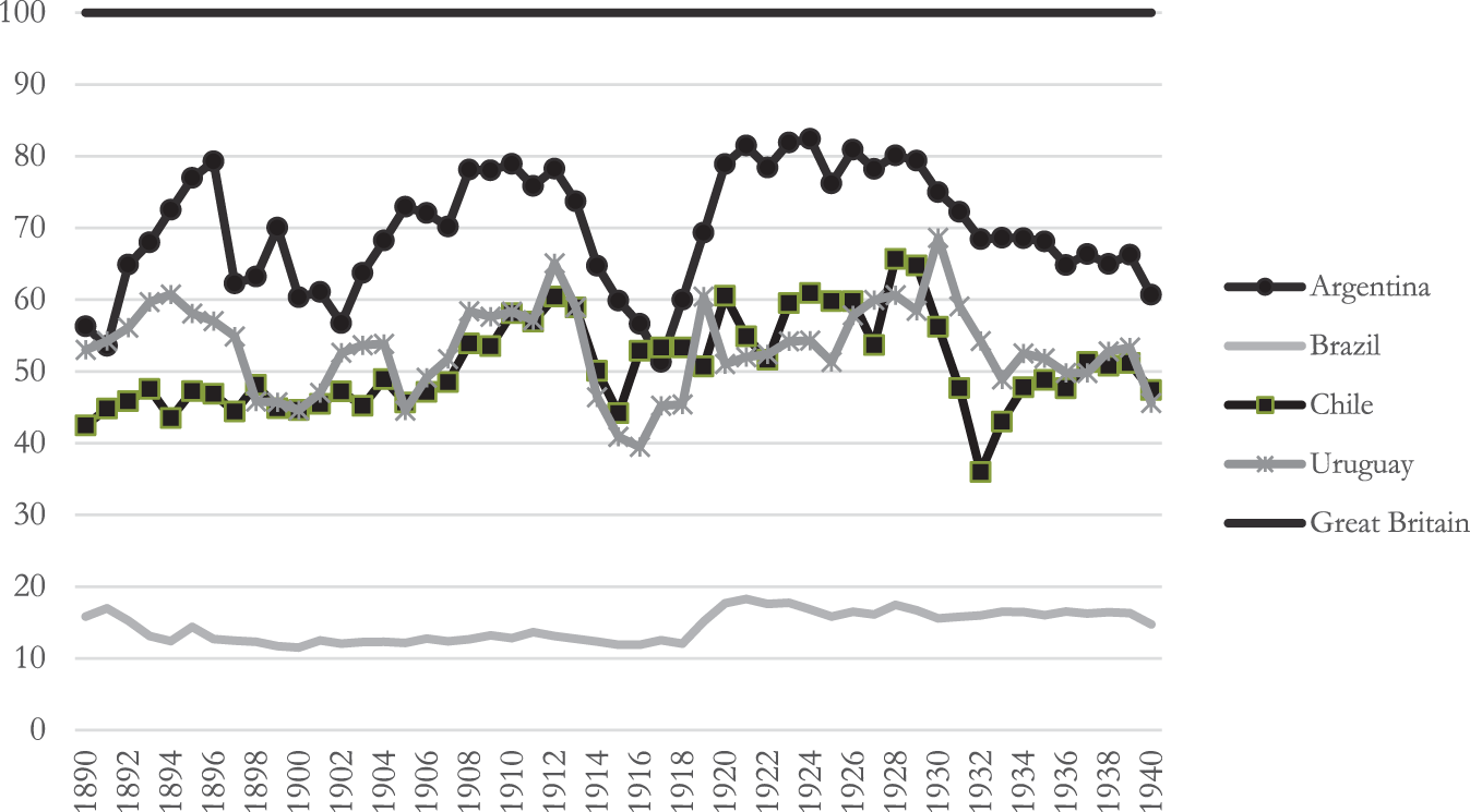
Another finding we would like to emphasise is the importance of using real wages to discuss living standards, at least during this period, rather than per capita GDP. Figure 4 illustrates per capita GDP of the Southern Cone countries relative to Great Britain (the figure is based on the Maddison Project Database).Footnote 78
Per capita GDP relative to Great Britain (Great Britain = 100)

Figure 4 Long description
A line graph showing per capita GDP relative to Great Britain (set at 100) for Argentina, Brazil, Chile and Uruguay from 1890 to 1940. The x-axis represents the years from 1890 to 1940 and the y-axis represents the GDP index. Argentina's line fluctuates between 50 and 90, peaking around 1910 and 1920. Brazil's line remains below 20 throughout. Chile's line varies between 40 and 60, with a dip around 1930. Uruguay's line fluctuates between 50 and 70, with peaks around 1910 and 1920. Great Britain's line is constant at 100. Each country is represented by a distinct line style and marker.
The figure illustrates that all the Southern Cone countries’ PPP-adjusted real wages remained below British levels. Argentina shows the highest levels, followed by Uruguay and Chile with similar trends. Per capita GDP of Brazil exhibited the lowest performance throughout the period. The divergence between Latin American countries in terms of GDP differs from the pattern for real wages. Overall, conclusions regarding the evolution of living standards cannot be fully understood if we solely rely on the aggregate GDP measure.
Conclusions
This article analyses living standards across cities in the Southern Cone of Latin America during a crucial period in their economic history, marked by the First Globalisation and the interwar years.
For this purpose, we constructed a set of PPPs for adjusting real wages in the capital cities of the Latin American Southern Cone – Buenos Aires, Rio de Janeiro, Santiago de Chile and Montevideo. The disparities we identified between the PLI and exchange rates underscore the need to adjust real wages in line with PPPs in order to avoid misleading conclusions. Our chosen strategy involved proposing new PPPs, developing two housing price scenarios, and offering a comprehensive description of the data and assumptions. This approach was selected to ensure a high degree of rigor and transparency. As with any method, ours has both advantages and drawbacks.
This paper improves on previous PPP estimates and offers new insights. We construct a new benchmark for 1938, provide more accurate data on food and rent prices than earlier studies, and present new estimates for Santiago de Chile and Rio de Janeiro. In addition, we develop alternative housing scenarios to compare rents for one- and three-room dwellings.
The main findings can be summarised as follows. The cost of the consumption basket was higher at the beginning of the twentieth century than during the 1930s, mainly due to the post-1914 decline in the relative prices of food and housing. The results show that (1) food was exceptionally expensive in Rio de Janeiro in 1905, and exceeding the costs in the other cities across all periods; and (2) in the pre-World War I era, housing costs in Buenos Aires, Montevideo and Rio de Janeiro were higher than those of comparable-sized dwellings in London. By contrast, Santiago de Chile consistently displayed lower housing costs than the other Southern Cone cities.
In terms of PPP-adjusted real wages, both Buenos Aires and Montevideo exhibited higher real wages compared to Rio de Janeiro or Santiago de Chile for both benchmarks. During the post-export-led growth period, real wages fell further behind those in London. Montevideo’s real wages were higher than those in Buenos Aires for the first benchmark but lower for the second benchmark. There was an unexpectedly high real wage for Santiago using the first benchmark, requiring an explanation, while a much lower real wage was observed in that city when the 1938 benchmark was used. Ultimately, real wages in Rio de Janeiro remained at 30–45 per cent of British real wages for both benchmarks.
In summary, we observe heterogeneous living standards in the cities of Latin America’s Southern Cone during the early twentieth century. This evidence is consistent with those studies (cited in the Introduction) that raise questions about the validity of the convergence hypothesis for the western side of the Atlantic Ocean. We found that the wage gap between the various Latin American cities analysed and London did not consistently decrease. In fact, after World War I, the deviation from London widened, and a growing gap emerged among the four Southern Cone Latin American cities.
To understand the persistent gap in living standards between the studied cities, it is crucial to consider other factors.Footnote 79 These include the dynamics of labour markets, the extent of informality, and labour force regulations. Differences in productivity, which depend on capital investment, as well as export sector specialisation (tropical products, mining or agriculture), also play a role. These sectors can vary in their capital intensity or reliance on labour (both in terms of quantity and qualifications). Additionally, the availability of workers – whether their supply is limited or unlimited – and the impact of terms of trade, which shift depending on the export product and international market dynamics, should be considered. Another significant aspect for consideration is the extent to which the results obtained for the capital cities can be generalised to other cities.
Lastly, it is important to acknowledge that PPP calculations are influenced by variations in prices and exchange rates. In this regard, a detailed discussion of monetary policies, balance of payments and terms of trade is essential. All these aspects remain topics for further research.
Supplementary material
The supplementary material for this article can be found at https://doi.org/10.1017/S0022216X26101370.
Acknowledgements
This research was undertaken as part of the HI-POD Project (Historical Patterns of Development and Underdevelopment: Origins and Persistence of the Great Divergence) supported by the European Commission’s 7th Framework Programme for Research. It was also part of the Research Group ‘Desarrollo Económico y Social de América Latina en Perspectiva Comparada’ supported by the Comisión Sectorial de Investigación (CSIC), Universidad de la República, Uruguay. Different stages of this paper have been presented in previous conferences, and we benefited from the comments received. We would like to thank especially J. Baten, S. Broadberry, M. Camou, E. Frankema, A. Herranz, M. Matus, E. Nicolini, J. Rodríguez Weber, R. Schmit, J. L. van Zanden, H. Willebald and J. Williamson for their suggestions. We are also very grateful to J. L. Martirén, M. Matus and E. Nicolini for sharing information with us and for their advice. The authors gratefully acknowledge the constructive feedback provided by the reviewers, the Editors, and the copy editor, whose comments and suggestions greatly improved this manuscript. Any remaining errors are our own.