2 Google Trends in Academic Research

GT has become popular in academic research in recent years. It was initially used in the late 2000s as a tool to analyze trends and monitor the evolution of diseases, viruses, or financial markets. Over time, the focus of research has shifted to forecasting (Jun, Yoo, and Choi Reference Jun, Yoo and Choi2018). Pelat et al. (Reference Pelat, Turbelin, Bar-Hen, Flahault and Valleron2009) track the evolution of the flu and diarrhea, while Carneiro and Mylonakis (Reference Carneiro and Mylonakis2009) use GT to monitor disease outbreaks in real time. Vosen and Schmidt (Reference Vosen and Schmidt2011) build a new indicator of private consumption based on data from GT. Examples of forecasting include Preis, Moat, and Stanley (Reference Preis, Moat and Stanley2013), who try to find “early warning signs” for stock market moves through changes in Google search volumes, Teng et al. (Reference Teng2017) dynamic model to forecast Zika epidemics, and Zhang et al.’s (Reference Zhang2018) forecast of seasonal infections.Footnote ² Lazer et al. (Reference Lazer, Kennedy, King and Vespignani2014), on the other hand, show the limitations of using GT to predict flu virus outbreaks.

In political science, we know of two noteworthy applications. First, Mavragani and Tsagarakis (Reference Mavragani and Tsagarakis2016) use GT to predict referenda outcomes in Europe from 2014 to 2017.Footnote ³ The authors calculate the share of “yes” and “no” searches (in each language) in the weeks leading up to the referendum and show that the percentages closely match the final outcome. The manner in which they transform GT data into percentages for or against a referendum question is not clear, and the approach is limited to dichotomous phenomena (such as yes/no votes). Nevertheless, the research shows the applicability of GT data to crucial democratic processes. Second, Chykina and Crabtree (Reference Chykina and Crabtree2018) measure issue salience for populations that are very difficult to sample using traditional survey techniques. They show how GT data can identify concerns by unauthorized immigrants about deportation from the United States in the aftermath of proposed policy changes and Trump’s election by using the search term “will I be deported.” With this method, they are able to identify key anti-immigration events: the passage of Arizona’s SB1070 law, Trump’s election and inauguration, and the Muslim travel ban imposed by the new President in early 2017. The authors also exploit GT’s geographic search tool to show that a majority of searches came from states with large illegal immigrant populations: California, Texas, and New York.

This growing body of work has discussed many of the challenges inherent in GT’s data generation process. First, Google search trends can be responsive to media trends rather than the underlying phenomenon of interest (Lazer et al. Reference Lazer, Kennedy, King and Vespignani2014). Second, GT results can be sensitive to apparently modest changes in search terms, and this is particularly stark when it comes to rare, but important, events like protests. Third, the underlying Google search and GT algorithms are under constant revision, and this can affect results. Despite these pitfalls, some extant work demonstrates the potential of Google searches to predict human behavior, such as Brigo et al.’s (Reference Brigo2014) study showing that people search for epilepsy-related terms to aid initial self-diagnosis. Similarly, we suspect that people interested in protesting use Google’s search engine to find information about where and when to do so.

3 How Google Trends Works

Any use of GT for research purposes requires careful consideration of how it is put together. It ostensibly tells us how popular a given term was on Google’s main search engine for a specific time frame and location. GT allows users to download data at the country, state, regional, metro area, and city levels. Metro area and city are only available in the United States, while regional data are available around the world in a country’s main first political subdivision. GT data are available from 2004 to the present. Users can specify the time frame (or window) for which they want to collect GT data—a few hours, a day, a week, a few months, or years. Time blocks, or the frequency over which the data are analyzed across the time frame, can be hourly, daily, weekly, or monthly, depending on the length of the time frame.Footnote ⁴ For time frames of up to 1 week, GT reports hourly data; for time frames of 9 months or less, daily data; for time frames between 9 months and 5 years, weekly data; and for time frames of greater than 5 years, monthly data. Researchers can access GT data in multiple ways, including R, Python, and Google’s own Trends application programming interface (API).Footnote ⁵ Note that Google’s search engine dominates in most markets worldwide, with market shares of 87.6% in the United States, 90% in Canada, and 97% in India, among others.Footnote ⁶ Data from some countries, most notably China, are not available due to internet restrictions.

To generate the GT data a user receives, Google first draws a random sample of all search traffic on its service for the requested location and time period. Google justifies producing results from samples instead of all search data on efficiency grounds.Footnote ⁷ This sampling process creates variability in the results from multiple, identical requests to Google’s API. This variability is particularly severe for low-volume search terms, which may not register in some of the sample draws. Thus, the same GT search for the same place and hour can generate somewhat different results (Choi and Varian Reference Choi and Varian2012).

Second, from this sample, Google’s algorithm calculates the “share” of overall traffic that the term represents, but it does not make that data available.Footnote ⁸ Instead, it transforms these “shares” of overall volume into a normalized index that ranges between 0 and 100.Footnote ⁹ A score of 100 indicates the time block when the search term was at its most popular during the time period under examination—that is, when the search term achieved its greatest share of overall Google search traffic (Choi and Varian Reference Choi and Varian2012). Thus, every search term will achieve a value of 100 at some point over the time frame of the GT search. GT then indexes the rest of the time blocks over the entire time period in reference to this highest point. If a time block has half of the highest hour’s volume, it receives a score of 50; if another time block has 100 times lower volume or less, it receives a score of 0. All other values within a time frame are indexed in relation to the highest value of 100, and thus receive scores between 0 and 99, inclusively.Footnote ¹⁰ Thus, the GT indexed score for a search term reflects its popularity in relation to itself over the time frame in a given location.Footnote ¹¹

This indexing has three important implications for researchers. First, it makes GT a poor tool for assessing a search term’s overall volume or popularity relative to other search terms. All search terms obtain a score of 100 at some point during a given search period even if the term represents a small share of overall search volume. Second, GT results can be very sensitive to the time frame over which the index is constructed. A typically low-volume search term, such as “protest,” will always generate a 100 score, even over time frames when protests are not salient. And those “100” scores are not easily distinguishable from “100” scores that the term “protest” would achieve during the Arab Spring or the Freddie Gray riots in Baltimore. Thus, any single GT search can be deceptive with regards to a term’s overall salience among Google searchers. Third and relatedly, while GT indexing does require that even low-volume searches achieve a 100-point score over a time frame, it does not necessarily assign the lowest volume time block for a search term a “0.” A search for popular terms such as “Trump” or “Gmail,” for instance, will not yield a 0 GT score in any time block. Conversely, a search for a low-volume term will always yield a 100 score (assuming there is enough data to produce a trend). An important implication is that high-volume searches will have less variance in GT scores than low-volume searches on average, even when the underlying distribution of raw searches have equal variance. This feature means that GT is particularly well-suited for detecting rare events, such as protests, because exaggerated pre-event interest will be reflected in reduced variation in GT scores. We exploit this feature below.

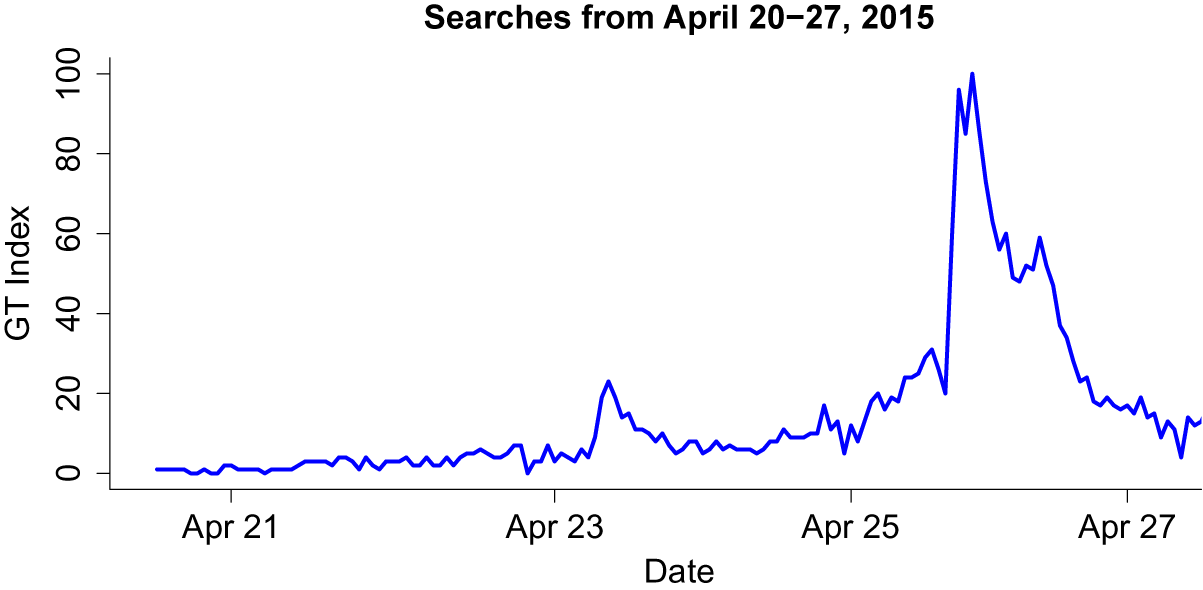
Figure 1 provides an example to elucidate these points; it plots the GT score of the word “protest” in the Baltimore metro area between April 20 and 27, 2015, when violent protests shook the city in the wake of Freddie Gray’s death at the hands of the police. In this example, we have hourly time blocks over the time frame of April 21–27. Since the time blocks are hours, we have a total of 168 data points (24 hours for each of the 7 days) for the term “protest” in Baltimore. The large spike in interest in the night of April 25 roughly coincides with the most violent episodes of the week—the Baltimore “uprising” or “riots.” Interest was relatively low earlier in the week and picked up slightly on April 23, the day of the first large, but nonviolent, protest.

Figure 1

Hourly Google Trends scores for “protest” (April 20–27, 2015—Baltimore metro area).

Notice that the y-axis is bound between 0 and 100. As described above, this is a function of how Google builds the GT index. First, GT assigns a value of 100 to the hour with the highest level of search volume for “protest” within the overall time frame. In this case, “protest” was most googled in Baltimore between 6 and 7 pm Eastern on April 25. We cannot know protest’s share in overall Google search volume in Baltimore during that hour, but we know it was at its highest share of all searches that week. Hence, GT assigns that 1 hour a score of 100. GT indexes the rest of the hourly scores for the week in reference to this highest point. For instance, on April 23 between 2 and 3 pm—the first small peak of the week—searches for “protest” represented one-third of the search volume of the week’s most popular hour (again, April 25 between 6 and 7 pm).

This example also helps clarify why GT data are poor for assessing a search term’s overall popularity relative to all search terms. For rare search terms, an index of 100 is achieved even with low absolute search volume. Imagine, for instance, that searches for “protest” were 23% of all search traffic on Google in Baltimore between 6 and 7 pm on April 25, 2015. Twenty-three percent is reflective of an objectively popular search term across all Google searches, but that is not what GT reports. Because 23% is also the peak popularity of “protest” searches over the April 21–27 period, GT produces a score of 100 for April 25 between 6 and 7 pm, and all other time blocks are indexed against it. However, some other objectively unpopular term—say “David Foster Wallace”—could also receive a score of 100 for April 25 between 6 and 7 pm, even if it peaked at only 2% of total search, as long as that hour was when “David Foster Wallace” was most searched over the time period.Footnote ¹²

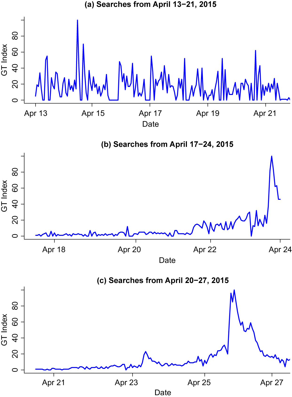
Figure 2, on the other hand, shows how GT indexing makes any single GT search very sensitive to the time frame of analysis, and thus, potentially deceptive. The figure shows hourly output on GT for the weeks of April 13–21 (a), April 17–24 (b), and April 20–27 (c), and all of 2015 in the Baltimore metro area for the search term “protest.” Plot (a), like the others, has one peak of 100 on April 17, but the variation is high across the period. Two other peaks are close to the 100 mark on early April 13 and late April 20. Notice that the peak from (a) disappears in (b), as April 17 search volume now pales in comparison to the peak of April 24. Variation is much lower, indicating that the surge of April 24 could potentially constitute an event. However, as shown in (c), that peak itself is much smaller than the one on April 25 at night (7 pm EST), the day of the riots. Thus, one snapshot of GT data will always produce a high point of 100, but whether that peak is constitutive of an important event is difficult to tell from any single capture. This indexing adds a layer of difficulty in utilizing GT data. Our approach, described below, exploits variance in a search term’s own trend to circumvent the limitations inherent in one-off GT results.Footnote ¹³

Figure 2

Hourly Google Trends scores for one protest over three different search periods (April 2015, Baltimore metro).

4 Event Detection and Forecasting

Potentially, one of the most promising applications of GT for the purposes of political scientists involve “event” detection and prediction. An event is an instance of a given phenomenon that takes place in a specific location for a finite period of time. In the event detection and prediction literature, researchers typically code events as involving an initiator (which could be anything from a person to the police to a country), a target (ditto), a magnitude, and a location (Gerner et al. Reference Gerner, Schrodt, Francisco and Weddle1994; Schrodt and Gerner Reference Schrodt and Gerner1994; King and Lowe Reference King and Lowe2003). There are large machine learning projects, including GDELT (Leetaru and Schrodt Reference Leetaru and Schrodt2013) and ICEWS (Boschee et al. Reference Boschee, Lautenschlager, O’Brien, Shellman, Starz and Ward2015), that aim to turn the world’s news into event data on everything from international conflict to mentions of specific world leaders. Other approaches rely on human coding of news and qualitative research to detect everything from protests (Fisher et al. Reference Fisher2019) to insurgent attacks (Raleigh et al. Reference Raleigh, Linke, Hegre and Karlsen2010) to international crises (Brecher et al. Reference Brecher, Wilkenfeld, Beardsley, James and Quinn2016). Event data have been used to model an enormous range of outcomes in the social sciences. Given Google search’s ubiquity around the world, we believe it offers some important advantages for event detection and prediction.

Most importantly, GT can overcome some important challenges and limitations in current sources for event data. First, GT can improve on the frequency of most event data. While some such data are reported at the annual level (Sarkees and Wayman Reference Sarkees and Wayman2010), others are more fine-grained, but rarely get better than daily (Leetaru and Schrodt Reference Leetaru and Schrodt2013). Properly tuned GT can report data at the hourly level. While this might not be useful for all social scientific enterprises, there are some (such as protests or financial markets) where hours can be crucially important; in some areas of research, the availability of higher frequency data might unveil analytical puzzles heretofore unexplored. Second, much event data in political science are reported at the national level and thus lack geographic nuance. In many cases, GT allows researchers to access at least the first subnational divisions within countries. Third and perhaps most importantly, GT overcomes some of the challenges inherent in more curated big data approaches that rely on the news. The challenges are myriad, including bias in underlying news sources, choosing which sources to rely on, developing and updating actor dictionaries, and deduplicating reporting of events across multiple sources (Schrodt Reference Schrodt2012; Grimmer and Stewart Reference Grimmer and Stewart2013; Leetaru and Schrodt Reference Leetaru and Schrodt2013; Lucas et al. Reference Lucas, Nielsen, Roberts, Stewart, Storer and Tingley2015). These challenges have resulted in a number of disagreements in empirical work on everything from the extent of reporting bias (Weidmann and Ward Reference Weidmann and Ward2010; Weidmann Reference Weidmann2016; Hollenbach and Pierskalla Reference Hollenbach and Pierskalla2017) to the utility of rules-based approaches over more advanced natural language processing techniques (Schrodt Reference Schrodt2012; Schrodt, Beieler, and Idris Reference Schrodt, Beieler and Idris2014). By relying on billions of Google searches and a clear understanding of how GT indexes, GT sidesteps many of these problems and offers the possibility to detect all manner of events that individuals around the world care about, including general elections, protests, police crackdowns, important legal changes, etc.

Below we focus specifically on identifying and forecasting protests using GT. There are two reasons for this choice. First, there is a lot of ground-truthed data on protest events, which aids with the development of models for event detection and forecasting (Fisher et al. Reference Fisher2019). Second, a large body of work has explored the predictors of protest, instability, and civil violence using in-sample and out-of-sample forecasting (Gurr and Lichbach Reference Gurr and Lichbach1986; Fearon and Laitin Reference Fearon and Laitin2003; Goldstone et al. Reference Goldstone2010; Ward, Greenhill, and Bakke Reference Ward, Greenhill and Bakke2010; Hegre et al. Reference Hegre, Karlsen, Nygård, Strand and Urdal2013; Cederman and Weidmann Reference Cederman and Weidmann2017; Chenoweth and Ulfelder Reference Chenoweth and Ulfelder2017; Bowlsby et al. Reference Bowlsby, Chenoweth, Hendrix and Moyer2020). These works use different structural and microlevel predictors to issue forecasts, but the predictive power of these variables inevitably varies over time. A strong predictor in 1980 may not be a strong predictor today (Bowlsby et al. Reference Bowlsby, Chenoweth, Hendrix and Moyer2020). One advantage of using data from GT is parsimony. Accurately predicting protest outbreaks using intensity, and variation in search interest over time for only one keyword simplifies the model substantially and, most importantly, should be consistent across time (Bowlsby et al. Reference Bowlsby, Chenoweth, Hendrix and Moyer2020). It also circumvents challenges inherent in text-based approaches using other sources of big data, such as Twitter, to predict protest outbreaks (Korolov et al. Reference Korolov2016; Bahrami et al. Reference Bahrami, Findik, Bozkaya and Balcisoy2018). Despite recent progress, tweets remain especially difficult for machines to filter and classify (Zhou, Chen, and He Reference Zhou, Chen and He2015). Given its ubiquity and often superior geolocalization,Footnote ¹⁴ Google search data might also offer more advance notice of impending events than Twitter, which has proved fairly accurate at forecasting a day or two ahead of protests. All told, our focus on temporal variation in a single search term on GT approach is more parsimonious than current models.

Lastly, while our focus is on event detection and forecasting, there are other creative applications of GT in political science worth mentioning. One is the ability to survey populations using search strings that only specific groups of people are likely to use as in Chykina and Crabtree (Reference Chykina and Crabtree2018). Another application involves creating proxies for common, important, but infrequently and/or misreported variables such as unemployment. Chadwick and Şengül (2013), for instance, show that GT is successful at nowcasting (i.e., predicting present values) of the nonagricultural unemployment rate in Turkey, which is only officially reported at monthly frequency. Finally, GT can reveal public attitudes without the expense of large sample surveys. Mavragani and Tsagarakis (Reference Mavragani and Tsagarakis2016), for instance, show how search volume on Google can reveal people’s preferences on political referenda and predict their result. These are a few examples of many potential applications of GT in political science, and we encourage further research along these lines. Whatever the application, it is important to approach GT with a clear understanding of how it works, since naive applications can produce misleading results.

5 The Variance-in-Time Approach to GT Data

We propose a “variance-in-time” approach to identifying and forecasting events using GT. The intuition behind the approach is that an analysis of high frequency and repeated samples of search terms can both successfully detect politically relevant events, even rare ones, and provide an important tool for forecasting them. Taking repeated samples of GT data over time allows us to incorporate variance into the analysis. Given the “black box” nature of GT indexing, focusing on consistency of interest rather than changes in the GT index itself can better reveal latent interest in an event (particularly a rare event) before it happens.

The “variance-in-time” approach consists of downloading GT data for all possible weekly combinations over a given time period. For our purposes, we collect data in 3-month periods, which have 82 full weeks, on average, with overlapping days.Footnote ¹⁵ In the case of Freddie Gray, the riots took place on April 25, 2015, between approximately 4 pm and 10 pm. We collect data between March 1 and May 31. The first week in the sample is March 1–March 7, the second is March 2–March 8, and so on until the last week of May 24–May 31. As described in a previous section, since data are collected in weekly windows, GT returns hourly data, so every week contains 168 data points after taking the mean for each hour.Footnote ¹⁶ After 7 days, each hour in the sample has been observed a total of seven times.Footnote ¹⁷ GT scores can change slightly, substantially, or stay the same for each data point every week, depending on whether the 100-point peak changes or stays the same. Each 3-month collection produces 13,776 data points.Footnote ¹⁸

After collecting the raw weekly data, we first take the mean $\mu $ GT index score for each hour in the sample. Calculating the mean serves to minimize the signal provided by any given “100” score that might result from the combination of low search volume and GT’s requirement that 1 hour in a week be indexed to 100.Footnote ¹⁹ We obtain a mean hourly GT index score for a total of 2,160 observations and calculate the standard deviation $\sigma $ in GT scores in 12-hour intervals. We use 12-hour intervals to maximize granularity while also allowing us to calculate meaningful standard deviations.Footnote ²⁰ In the context of GT, 12-hour periods are often long enough to detect meaningful change—many events see large increases and decreases in interest in windows of 12 hours or less.Footnote ²¹ Using the GT means per hour and the standard deviation, we then compute the coefficient of the variation for each hour, i.e., $\sigma /\mu $ .Footnote ²²

The coefficient of the variation helps us incorporate the variance in GT scores into our calculations and go beyond mean scores, which are inherently noisy when trying to detect rare events (like protests) in contexts of low search volume. The intuition here is that consistency of interest, and not just the level of interest, can both indicate as well as forecast an event. Given the nature of GT indexing, a topic may become more popular without its mean increasing very much, because another—and unrelated—peak of “100” may be drowning out the increase in the mean for the new event. Lower variance, on the other hand, will always reveal more consistent interest in a search topic, which in turn suggests that the topic is becoming more popular even if the mean GT score does not reflect that. Incorporating the variance helps us paint a fuller picture of search interest. Definitionally, holding the mean constant, the coefficient of the variation will be smaller when variation in search interest is low (smaller $\sigma $ ). When variance is high, the coefficient will be larger. Therefore, we expect a lower coefficient of variation to be associated with a higher probability of observing a given event—in our case, a protest.

Part of the reason for this expectation lies with the behavior of the mean $\mu $ . With a single sample of GT data, a high GT score can indicates broad interest in a topic, but it can also result from a small increase in interest in a context of low search interest. Recall that GT always produces a score of 100 for every collection, as it assigns 100 to the time block that had the highest share of searches among overall traffic on Google. If one collects data for a week where interest was quite low throughout, scores are likely to be abnormally high (say, around 50), because many hours will achieve “100” scores even without serious search interest. The hour with the most searches will receive a score of 100, but with rare events search volume in other hour blocks will be similar. This means that many hour blocks will receive relatively high GT scores, as they are indexed against the peak hour. Some will go to zero, because no search volume occurred. Thus, weeks with little interest have high GT means, rather than low ones, but most of this variation is a function of many different low search blocks actually achieving a “100” score. Conversely, when interest becomes more consistent, the mean will initially decrease. Consistent interest reduces the number of 100-point peaks driven by low-volume searches and lowers the values of other data points around a true spike. Hence, the mean will decrease when a search topic begins to garner interest. It will then increase again when interest is consistent and high, even though there will be fewer peaks of 100.

This fluctuation in the mean creates interesting dynamics in the coefficient of variation. A high mean will make the coefficient smaller. We expect higher means both in periods with low interest (noise) and when a rare event is likely to take place (i.e., true high interest), and lower means when the topic begins to attract attention on GT. Therefore, the coefficient should be largest when the issue receives very little attention on GT, become smaller as the issue becomes more popular, and be at its lowest values when attention is at its peak. In other words, the numerator ( $\sigma $ ) decreases as interest increases, and the mean evolves in a u-shape pattern: it is higher with low interest, lower with increasing interest, and high again with true high-volume interest.

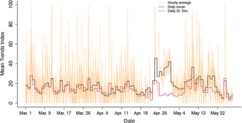
Figure 3 shows this graphically for the case of Freddie Gray. The orange line plots the mean GT scores for all hours between March 1 and May 31, 2015, as well as the mean and the variance for each day in the sample (red and black lines).Footnote ²³ The variance starts decreasing substantially around April 12, the day of Freddie Gray’s arrest. The hourly means follow a similar trajectory, before they increase again as the protests take place. Note the many cases of 100 point scores, even early in the month before any of the incidents bearing on the Gray protests took place; many of these high scores reflect GT indexing on a low-volume search. There is only one mean peak greater than 70 between April 12 and May 6 (the peak of April 25), but at least six in the month prior to April 12.

Figure 3

Means and variance over time in Baltimore, March 1–May 31, 2015.

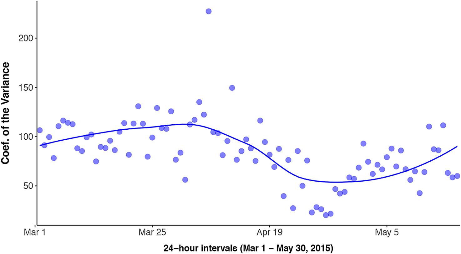
Figure 4 plots the resulting coefficient of the variation—the standard deviation over the mean. Points are much farther apart on the left side of the plot before April 12 (Day 43). After that, points are first closer to one another (lower variance) and then decrease sharply before and during the protest. Figures 3 and 4 show the potential of the coefficient of variation to detect and forecast a protest event days before the protest actually takes place. We can detect an event by observing multiple points in a sequence in which the coefficient of the variation is much lower than the expected trend (see Figure 4). In terms of forecasting, there are two aspects of Figure 4 that we can exploit: variance overall decreases after an initial positive shock to variance around April 4. We cannot issue a reliable forecast based on one event and build a generalizable model from it, but we think there is sufficient evidence in the Freddy Gray event to suggest that our approach to GT data may yield accurate forecasts. We develop a generalizable forecasting strategy in the next section.

Figure 4

Evolution of the coefficient of the variation in Baltimore, March 1–May 31, 2015.

6 Forecasting Protests in the United States

6.2 In-Sample Results

First, we fit a generalized linear model using the full sample of 568,080 observations with a set of lagged values of the coefficient of variation as the main predictors. We also add metro-area fixed effects. The coefficient of variation is lagged up to 5 hours before the protest event and then daily until 7 days before the protest date. Protest is dichotomous: days with protests are set to 1, and days without protests to 0.Footnote ³¹ The results are identical using a linear probability model—the sample size is so large that logistic regression coefficients remain largely unbiased even in the presence of a large number of parameters (Beck Reference Beck2020).

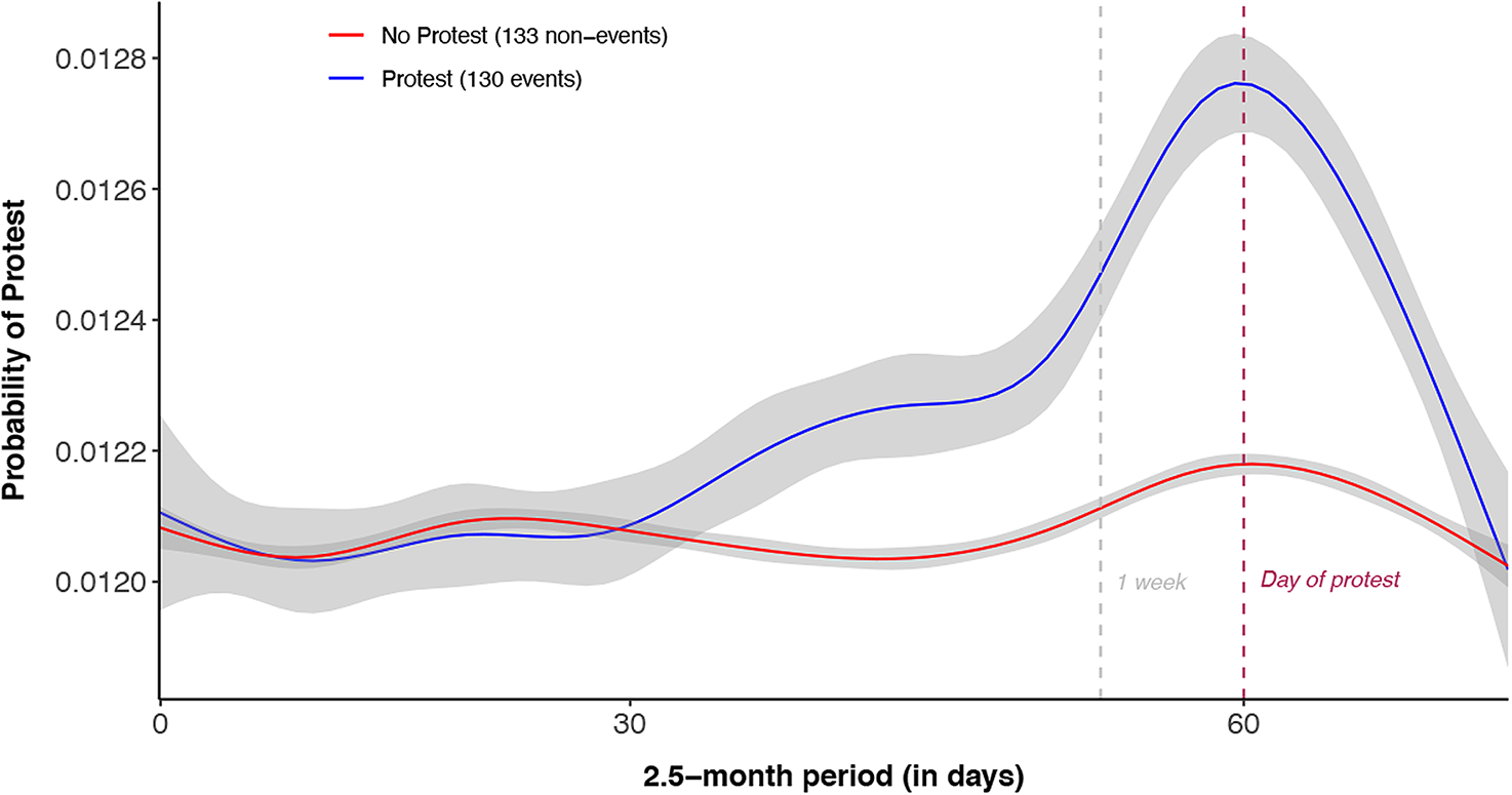
Figure 5 shows the predicted probabilities for protest and no protest groups based on the logistic model.Footnote ³² We refer to the protest subset as “positive” and the synthetic control as “negative.” The x-axis is days, and the predicted probabilities of protest are on the y-axis. All protests in the sample are set to take place on Day 60. The results are computed using the full model, not a split sample.Footnote ³³

Figure 5

Effect of the coefficient of the variation in Google Trends scores on protest.

The contrast between the predictions for our true protest sample and the synthetic control is striking. The model places the highest probability of protest in the positive group at the day of the protest. The probability of a protest is 7% higher in cities where a protest occurred in the data than in our control group, a statistically significant difference. Moreover, as Figure 5 shows, the probability curves for these two groups begin to diverge much earlier. Significant differences can be observed 1 and 2 weeks before the day of the protest. This creates an opportunity for predicting protests further ahead than current models Bahrami et al. (Reference Bahrami, Findik, Bozkaya and Balcisoy2018). On the other hand, the probability of protest for the control group is mostly flat for the entire period. It is also indistinguishable from the treatment group’s probability of protest between 1 and 2 months prior to the protest date.

6.3 Out-of-Sample Results

We apply a logistic regression classifier and use K-fold cross-validation to produce out-of-sample forecasts. We follow the literature in the selection of the model (Korolov et al. Reference Korolov2016; Bahrami et al. Reference Bahrami, Findik, Bozkaya and Balcisoy2018).Footnote ³⁴ The output of the logistic regression is the probability that a protest takes place in a metro area in a given time period. The classifier transforms the probability for each protest event into a binary value. We allow the algorithm to select a cutoff point to perform the conversion. The model assigns a 1 if the predicted probability is above the cutoff point and a 0 otherwise. Thus, the model’s output is a dichotomous variable that indicates whether a protest is predicted or not.

We use K-fold cross-validation to perform out-of sample forecasts setting the number of folds at 10.Footnote ³⁵ K-fold cross-validation divides the sample into 10 random splits, keeping 9 as training data and 1 as test data. For each unique group, we fit a model on the training data and evaluate it on the test set. We obtain a set of 10 different results, which we use to summarize the skill of the model. This procedure is particularly useful to test the skill of our model considering the relatively small sample size of protests. Recall that our final dataset for the forecasting model consists of 263 observations—130 protest events and 133 null events. A simple train/test split, in which we split the sample into training and test sets only once, generally yields more biased and optimistic estimates of model fit, a problem that is exacerbated in smaller samples (see Brownlee Reference Brownlee2018).

Our models test the predictive capacity of the coefficient of the variation on protest. The first model uses the maximum and minimum values of the coefficient of the variation between 1 and 3 weeks prior to the protest. These variables are aggregated at the protest level. For instance, if a protest took place on June 1, we would calculate the maximum and minimum values of the coefficient of the variation between May 7 and May 24. This effectively lags our prediction one full week (our previous in-sample model indicates this is highly predictive of a forthcoming protest). This lag shows that our model can forecast protests further in advance than current work, which usually issue 3-, 2-, and 1-day forecasts (Korolov et al. Reference Korolov2016; Bahrami et al. Reference Bahrami, Findik, Bozkaya and Balcisoy2018). In the model, we also include the maximum and minimum values between 3 and 5 weeks and 5 and 7 weeks prior to the protest.

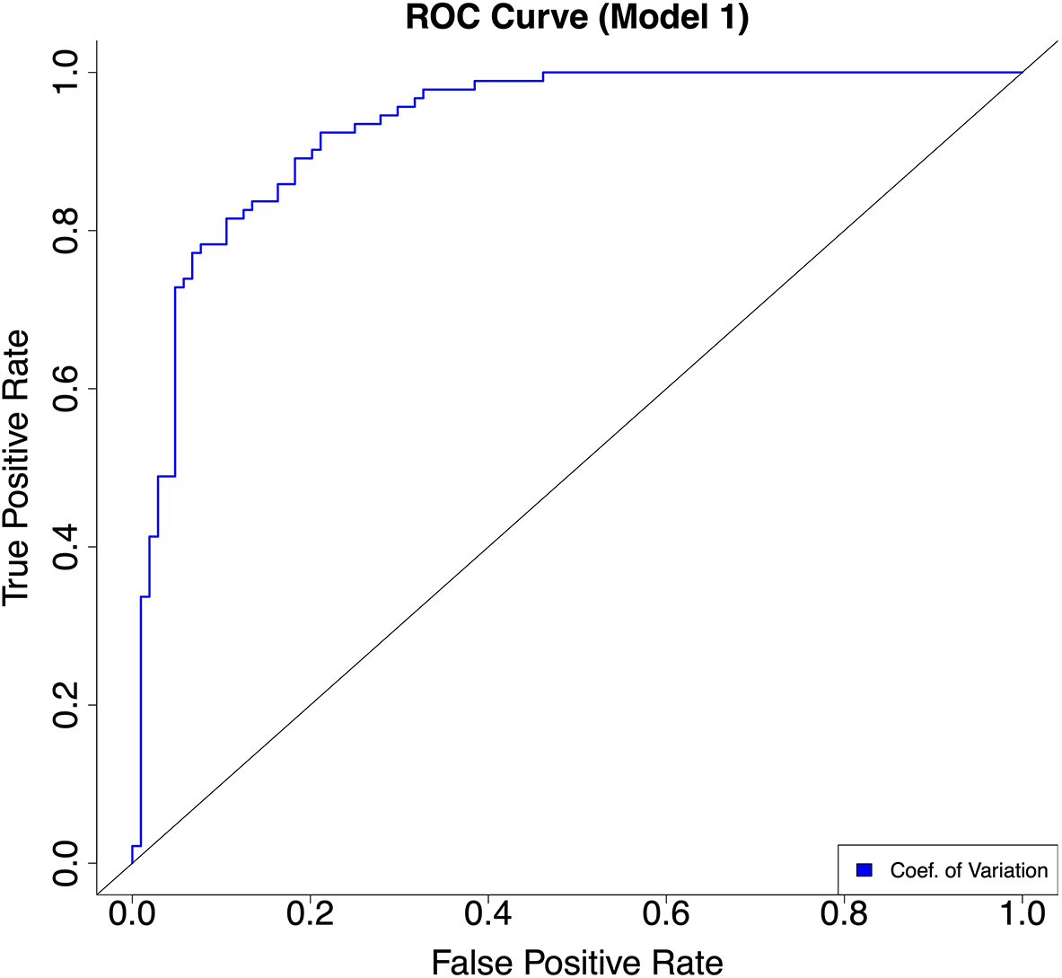
Figure 6 shows the area under the receiver operating characteristic (ROC) curve for the first model. The ROC curve illustrates the predictive capacity of a model, showing the trade-off between true positive and false positive rates as we vary the decision threshold. The area under the ROC tells us accurately a model classifies true positives. The closer it is to 1, the better the model performance. Here, Figure 6 provides strong evidence that the coefficient of variation can be highly predictive of protest events. The area under the ROC score for the main model is 0.92, while out-of-sample accuracy stands at 0.85, both high scores.Footnote ³⁶ Using the coefficient of variation, we are correctly predicting 85% of protests on unseen data. This translates into 110 protests correctly identified by the model for a recall of 0.88. We fail to predict 13 protests that did take place. Conversely, we are identifying 114 true negative events and incorrectly identifying 26 protests that never happened (false positives).

Figure 6

ROC curve (Model 1).

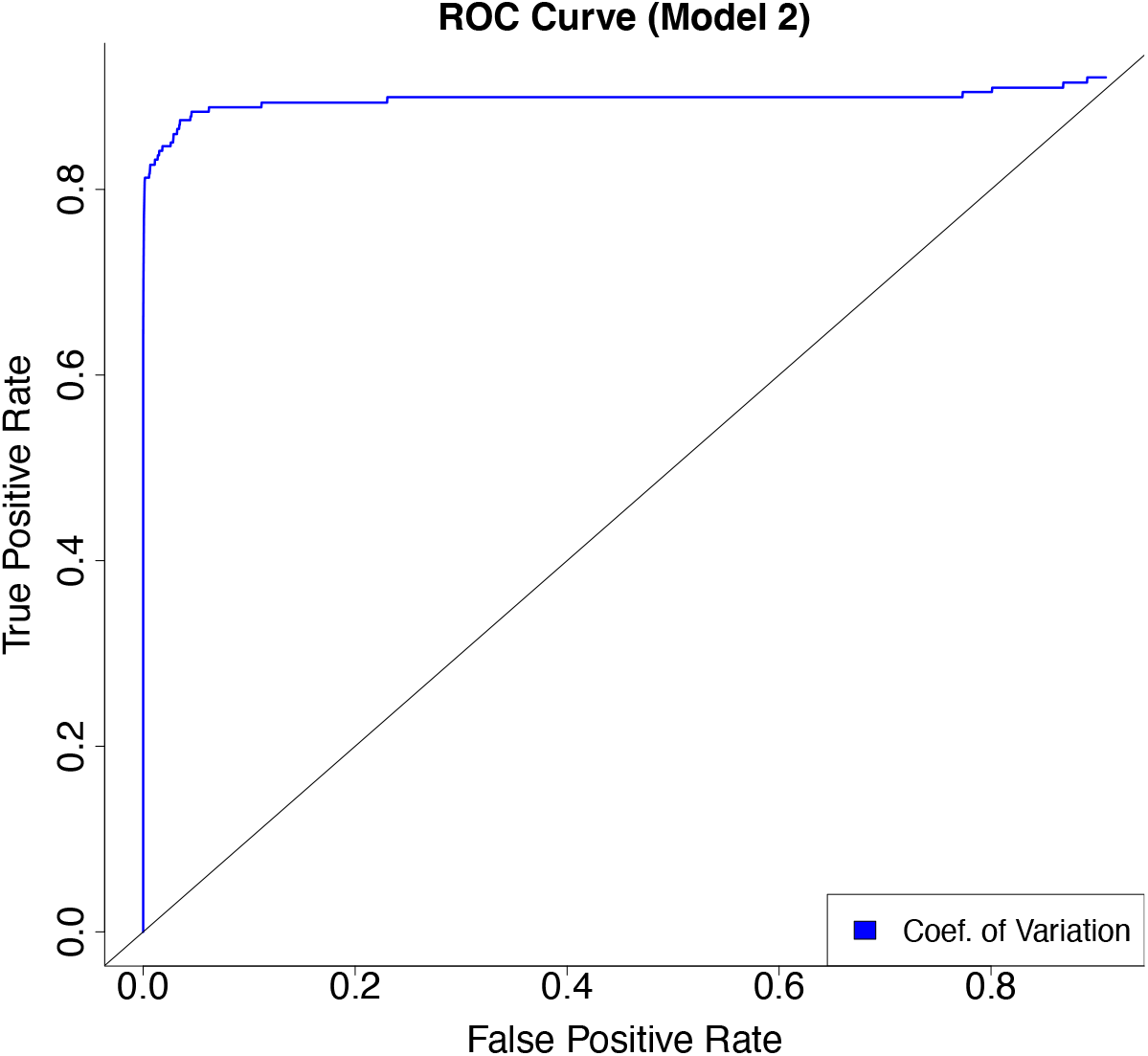
We build a second model that calculates daily protest probabilities per urban area and predicts the day when a protest is likely to take place. Our predictors are the coefficient of variation (logged) lagged from 1 to 14 days before the protest. Since protest events are rare in the training data (0.8%), we use gradient boosting (gbm) to circumvent known pitfalls of logistic regression with highly imbalanced outcome variables (King and Zeng Reference King and Zeng2001; Beck Reference Beck2020).Footnote ³⁷ Given rare events, accuracy scores are not a great tool to evaluate the model as high train and test accuracies are solely driven by correctly predicted zeroes.Footnote ³⁸ We thus turn again to area under the ROC scores and report the confusion matrix, both of which are more instructive of model performance. Model 2 has a mean area under the curve (AUC) score of 0.90, which again provides strong evidence of the power of the coefficient of the variation to predict protest events (Figure 7).

Figure 7

ROC curve (Model 2).

The confusion matrix confirms the strength of the model. A confusion matrix compares the predicted values of an outcome from a model versus the actual values in the data. We look for (1) a high number of matches between predicted true positives and actual true positives, and (2) a high number of matches between predicted true negatives and actual true negatives in the data. Over 10 folds,Footnote ³⁹ the model correctly predicts an average of 23.6 protest days in the test data and only fails to predict 6.4 known protest events (false negatives). 78.4 percent of protests are thus correctly identified, as are all nonprotest observations. Moreover, the model produces no false positives on average, leaving an $F_{1}$ score of 0.88. These results using gbm are especially strong considering how rare protest events are in the second dataset (130 out of 15,780 observations). The gbm model greatly improves on the performance of the logistic regression classifier, which does no better than random chance.

These findings show that the coefficient of variation can predict protest from GT data earlier than current models. For reference, we use innovative work by Bahrami et al. (Reference Bahrami, Findik, Bozkaya and Balcisoy2018) that leverages Twitter data to forecast protest events. The authors collected tweets between November 9 and 16, 2016, with hashtags related to protests against Donald Trump’s election and used machine learning to forecast when a protest was likely to take place. Their model predicts protests perfectly for November 15 and 16, dates in which protest events were common throughout the United States. Three days prior to these major events, however, their model issues protest probabilities around coin-toss levels. Our model manages to issue much more accurate forecasts up to a week in advance, leveraging small but detectable changes in Google search activity.