2.1. DNS with $Re_{\tau }=180$ and 395 at moderate rotation numbers

The presence of very long structures along the streamwise direction is one of the main characteristics of the present numerical simulations, and sufficiently long computational domains, especially in the streamwise direction, should be used to capture these long structures (Jiménez & Moin Reference Jiménez and Moin1991; Wu & Kasagi Reference Wu and Kasagi2004; Weller & Oberlack Reference Weller and Oberlack2006; Recktenwald et al. Reference Recktenwald, Weller, Schröder and Oberlack2007). Hence, at the present rotation numbers, we chose a largest computational domain with $128{\rm \pi} \times 2 \times 8{\rm \pi}$ in the streamwise, wall-normal and spanwise directions with $Ro_{\tau }= 30$ and $Re_{\tau }=180$. 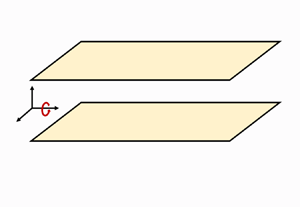Their definitions are $Ro_{\tau}={2\varOmega_x h}/{u_{\tau}}, Re_{\tau}={h u_{\tau}}/{\nu}$, and h is the half-channel height. The sketching diagram is shown in figure 1. In our numerical simulations, we use four rotation numbers of $Ro_{\tau }=0, 7.5, 15$ and 30 with a fixed Reynolds number based on the wall-friction velocity $Re_{\tau }=180$ to evaluate the rotation number effects, and compare the statistical consequences at a fixed rotation number $Ro_{\tau }=7.5$ with $Re_{\tau }=180$ and $Re_{\tau }=395$ to evaluate the Reynolds number effects. The corresponding mesh setting of the DNS with $Re_{\tau }=395$ at a weak streamwise rotation refers to Moser, Kim & Mansour (Reference Moser, Kim and Mansour1999) with a small computational domain.

Figure 1.

Sketch of turbulent channel flow with streamwise rotation.

Similarly, the rotation number and Reynolds number based on the bulk velocity are obtained by

(2.2a,b)\begin{equation} Ro_b=\frac{2\varOmega_x h}{U_b}, \quad Re_b=\frac{h U_b}{\nu}. \end{equation}

The bulk velocity is

(2.3)\begin{equation} U_b=\frac{1}{2h}\int_{{-}h}^h U(y)\,{{\rm d} y}. \end{equation}

The statistical analyses begin after the flows reach steady state, and we select the last $40h/u_{\tau }$ as the sampling time. Unless otherwise stated, all physical variables present in this paper are non-dimensionalized by the inner scale with the wall-friction velocity $u_{\tau }$ and the kinematic viscosity $\nu$, and they are marked by superscript symbol $+$. Some characteristic parameters are listed in table 1.

Table 1.

The computational configurations and some characteristic parameters of the flows.

We show the profiles of mean velocities in the streamwise and spanwise directions under different rotation numbers and Reynolds numbers in figure 2. Averaging is performed over the $x$–$z$ plane and time, which is marked by $\langle \cdot \rangle$. The statistical results are consistent with previous work (Yang et al. Reference Yang, Su and Wu2010; Yang & Wang Reference Yang and Wang2018), even though we adopted a larger Reynolds number. The inhibitory effects of the rotation number are reflected at the smaller mean streamwise velocity with higher rotation numbers. However, the statistical consequences of the mean spanwise velocity under different rotation numbers are slightly different from the results obtained in Yang et al. (Reference Yang, Su and Wu2010). The rotation number effects on the mean spanwise velocity distribution are monotonic in the present numerical simulations. With the increase of rotation number, the amplitudes of the reverse flow in the core regions are larger, and their peak locations are farther away from the channel centre. Likewise, the secondary flows close to the wall are also enhanced by higher rotation numbers. The Reynolds number effect is negligible in the near-wall regions, and the amplitudes of a mean secondary flow also increases with a higher Reynolds number. In contrast, there does not exist a secondary flow without rotation.

Figure 2.

The profiles of mean velocities in the streamwise and spanwise directions.

According to the homogeneity conditions in the streamwise and spanwise directions, the presence of a mean secondary flow leads to a non-zero-mean vorticity in the streamwise direction. Hence, the streamwise vorticity is also the main characteristic of turbulent channel flows with streamwise rotation. The profiles of mean vorticities in the streamwise $\langle \omega _x \rangle ^{+}$ and spanwise directions $\langle \omega _z \rangle ^{+}$ under different rotation numbers and Reynolds numbers are exhibited in figure 3. The mean wall-normal velocity and vorticity are zero, and we do not show their profiles in the current paper. In the present analysis, the mean streamwise vorticities are obtained by computing the slopes of the mean spanwise velocity vs wall-normal height $y$, and the mean spanwise vorticities are obtained by computing the slopes of the mean streamwise velocity vs wall-normal height $y$. For the mean streamwise vorticity in figure 3(a), there exists a peak within the half-channel. The peak is located around $y\approx \pm 0.8$, which is associated with the shoulder of the mean flows (Oberlack et al. Reference Oberlack, Cabot, Reif and Weller2006; Dai et al. Reference Dai, Huang and Xu2019). The shoulder locations are easily affected by system rotation, and the amplitudes of the mean streamwise vorticities are enhanced by higher rotation numbers. In addition, the peak locations move closer towards the wall with the increase of rotation number. From the peak towards the wall or channel centre, the streamwise vorticity decreases monotonically. Around the wall, its sign is negative and its amplitude is very large, which is caused by large gradients of spanwise velocity within the near-wall regions. Meanwhile, around the channel centre, its sign is also negative and the cosine distribution is consistent with the inertial waves solution (Yang et al. Reference Yang, Su and Wu2010). The inhibitory effects of streamwise rotation are also reflected in the profiles of the mean spanwise vorticity in figure 3(b). With the increase of rotation number, the amplitudes of the mean spanwise vorticity are weakened, especially around the shoulder location. The large mean spanwise vorticity can be attributed to the large gradient of streamwise velocity within the boundary layers. As for Reynolds number effect, a higher Reynolds number corresponds to a more fully developed turbulent state, and it leads to larger vorticities at the wall boundary. However, the vorticity profiles at the streamwise and spanwise directions are similar at different Reynolds number.

Figure 3.

The profiles of mean vorticities in the streamwise and spanwise directions.

2.2. Numerical simulations with higher Reynolds numbers through DNS and LES

The Reynolds number effects on the distributions of the mean secondary flows are worth exploring, and we carry out more numerical simulations with higher Reynolds numbers in this section. In order to be consistent with previous numerical settings, we adopted the LES method to investigate turbulent channel flows with $Ro_{\tau }= 7.5$ and $Re_{\tau }= 395$, 590 and 1000. The dynamic Smagorinsky model (Germano et al. Reference Germano, Piomelli, Moin and Cabot1991) is employed, and this model has been claimed to be successful for turbulent channel flows with streamwise rotation (Dai et al. Reference Dai, Huang and Xu2019). In addition, DNS with a weak rotation number $Ro_{\tau }= 2$ and $Re_{\tau }= 1000$ and 2000 are also carried out to explore the Reynolds number effects. In order to decrease the computational cost, we select developed turbulent channel flows without any rotation as the initial flow fields. The raw dataset with $Re_{\tau }= 1000$ was downloaded from the Johns Hopkins Turbulence Database (JHTDB)(see http://turbulence.pha.jhu.edu) (Graham et al. Reference Graham2016), and another raw dataset with $Re_{\tau }= 2000$ was downloaded from the website of the University of Texas at Austin (see https://turbulence.oden.utexas.edu/) (Hoyas & Jiménez Reference Hoyas and Jiménez2006). The specific parameters including the computational domains, mesh cells, Reynolds numbers and rotation numbers are listed in table 2.

Table 2.

The computational settings and characteristic parameters of the flows with higher Reynolds numbers through DNS and LES.

The mean streamwise and spanwise velocity profiles with the LES method are exhibited in figure 4, and the mean streamwise and spanwise velocity profiles with $Re_{\tau }= 395$ through the DNS method are compared to verify the success of the current LES model. For the streamwise velocity profile, the discrepancies are negligible except in the core regions with different Reynolds numbers. For the spanwise velocity profile, the mean secondary flows are preserved with different Reynolds numbers. The main difference lies in the locations of peak and valley, and their locations move away from the wall with increasing the Reynolds number.

Figure 4.

The profiles of mean velocities in the streamwise and spanwise directions with $Re_{\tau }=395$, 590 and 1000. The mean streamwise and spanwise velocity profiles with $Re_{\tau }=395$ are compared with symbol $\circ$.

For the case with higher Reynolds number and a weak rotation number using the DNS method, we show the profiles of the mean streamwise and spanwise velocity profiles at different typical instants in figure 5 to investigate the effects of the presence of the streamwise rotation on the development process of the secondary flows. For the mean streamwise velocity profiles, the initial distributions are consistent with classical scaling laws with $Re_{\tau }$ = 1000 and 2000, and they assure us of the quality of the datasets we downloaded. With the presence of the streamwise rotation, the mean streamwise velocity profile begins to depart from the initial distributions. In the meanwhile, the mean spanwise velocity profile begins to develop, up to regular distributions of the secondary flows. With time, the system rotation drives a wall-normal transfer of spanwise momentum. The mean secondary flows begin to form within the near-wall regions, and then develop at the core regions. The development processes of the secondary flows are similar with $Re_{\tau }$ = 1000 and 2000, and eventually towards a stationary status. We highlight the presence of the mean secondary flows with high Reynolds numbers, and the statistical analysis of the stationary flow fields turns to the case with smaller Reynolds numbers and moderate rotation numbers.

Figure 5.

The profiles of mean velocities in the streamwise and spanwise directions at different typical instants with $Re_{\tau }= 1000$ and 2000.

The above statistical consequences reveal that the secondary flows are common at different Reynolds numbers, and the Reynolds number effects are mainly reflected in the locations of the peaks and valleys of the secondary flows. Nevertheless, the rotation number effects are the main factor for the secondary flows and are more complicated (Yang et al. Reference Yang, Su and Wu2010; Yang & Wang Reference Yang and Wang2018), and we select the cases with $Re_{\tau }=180,395$ at moderate rotation numbers to explore the helicity distributions and scale transfer in the following sections.

3.1. Helicity profiles

To further investigate the transfer paths of energy and helicity with background shear flows, we can decompose the fluid fields into mean and fluctuating components as $a=\langle a \rangle +a'$ (Härtel et al. Reference Härtel, Kleiser, Unger and Friedrich1994; Piomelli, Yu & Adrian Reference Piomelli, Yu and Adrian1996), and the fluctuating components can be further decomposed into resolved and unresolved components. In contrast to homogeneous and isotropic turbulence, new energy transfer paths exist for mean flows decomposed into resolved and unresolved components in wall-bounded turbulent flows. In this section, we show the mean and fluctuating components of energy and helicity to characterize the flow field. The resolved and unresolved components analysed by the filtering method are emphasized in a later section.

We can define the mean and fluctuating energy as

(3.1a,b)\begin{equation} Em=\langle u \rangle^2+\langle w \rangle^2, \quad Ef=u'^2+v'^2+w'^2. \end{equation}

Similarly, the mean and fluctuating helicity can be defined as

(3.2a,b)\begin{equation} Hm=Hxm+Hzm=\langle u \rangle \langle \omega_x \rangle+\langle w \rangle \langle \omega_z \rangle, \quad Hf=u' \omega_x' + v' \omega_y'+ w' \omega_z'. \end{equation}

Here, the prime $'$ denotes a fluctuating component. It should be mentioned that there exist another two components consisting of mean and fluctuating fields according to the Schwarz inequality. However, their ensemble averages are zero, and they are absent in the above decompositions.

The profiles of mean and fluctuating energy and helicity are shown in figure 6. The profiles of the mean energy are consistent with the distributions of streamwise velocity in figure 2. The main reason for this is that the streamwise velocity is dominant, even though there exists a mean secondary flow of the spanwise velocity. In the core regions, the amplitudes of the mean energy decrease with an increase of rotation number. However, the rotation effects on the fluctuating energy are different. With the presence of streamwise rotation, the fluctuating energy profiles are indeed changed, but rotation number effects are not monotonic in the near-wall regions. With the increase of rotation number in the core regions, the amplitudes of the fluctuating energy would increase. Hence, we can conclude that rotation would promote the energy path from the mean flows into fluctuating flows in the core regions. The Reynolds number effects on the fluctuating energy profiles are similar in the core regions. The mean and fluctuating helicity are nearly zero in turbulent channel flows without rotation, which verifies the necessity of exploring helicity statistics in turbulent channel flows with streamwise rotation. The profiles of the mean helicity in figure 6(c) indicate uniform helicity distributions of the main flows. With the increase of rotation number, the amplitudes of the mean helicity increase gradually in the core regions. In the near-wall regions, the amplitudes of helicity also increase with the increase of rotation number. Meanwhile, the peaks of the mean helicity distribution gradually approach the wall. The positive and negative helicities in different regions mainly depend on the mean spanwise velocity. We show the fluctuating helicity profiles at different rotation numbers in figure 6(d). The rotation effects are similar to those of the mean helicity. However, with a higher Reynolds number, the amplitudes of the mean and fluctuating components of helicity are larger with similar profile distributions, even at a weak rotation number. This means that high helicity might exist and be apparent in turbulent flows with high Reynolds numbers. In the present numerical simulations, the larger helicity profiles are obtained by relatively large streamwise rotations at relatively low Reynolds numbers, and the regulations might be extended to natural or engineering turbulent flows with higher Reynolds numbers. The regular distributions pave the way for exploring the spectra and fluxes of helicity in later sections.

Figure 6.

The profiles of the mean and fluctuating energy (a,b), and the mean and fluctuating helicity (c,d).

To investigate the helicity anisotropy in turbulent channel flows, we show the mean helicity profiles in the streamwise (Hx) and spanwise (Hz) directions in figure 7. Energy anisotropy has been explored in turbulent channel flows (del Alamo & Jiménez Reference del Alamo and Jiménez2003; Dunn & Morrison Reference Dunn and Morrison2003; Jiménez Reference Jiménez2012), and we apply the methodology to helicity anisotropy. The mean wall-normal helicity is nearly zero, because the mean velocity and vorticity in the wall-normal direction are zero in turbulent channel flows, and we do not show their profiles for the sake of simplicity. Except for the peaks nearest to the wall, the profiles of the mean streamwise helicity are similar to the total helicity profiles in figure 6, both in terms of amplitudes and peak locations. However, new larger peaks of the mean streamwise and spanwise helicity exist around $y^+=6$ with $Ro_{\tau }=30$. As for the cases with weak rotation, the peak locations may be larger, but all of them are smaller than the locations of the buffer layers. Their amplitudes are nearly the same, but their signs are different. Hence, the newly found peaks in the near-wall regions are not easily found in turbulent channel flows (Nguyen & Papavassiliou Reference Nguyen and Papavassiliou2020). The presence of the new peaks can be attributed to the mean large vorticity in the near-wall regions. Dimensional analysis of the amplitudes of the mean streamwise velocity and vorticity, and the mean spanwise velocity and vorticity in the near-wall regions in figures 2 and 3, can also verify the relationship of the amplitudes of the mean streamwise and spanwise helicity. The newly found peaks indicate a high helical status in the near-wall regions, which also can be characterized by Taylor–Görtler-like vortices at the cross-section perpendicular to the streamwise direction in figure 8(b). In figure 8(a), the large-scale Taylor–Görtler vortices characterize the helical structures beyond the near-wall regions. The spiral characteristic represented by wall-normal and spanwise velocity vectors, accompanied by the mean streamwise velocity, reflects the three-dimensional helical structures.

Figure 7.

The profiles of the mean helicity in the streamwise direction (a) and the spanwise direction (b).

Figure 8.

(a) Taylor–Görtler vortices visualized by the contours of the fluctuating streamwise vorticity and velocity vectors in the wall-normal and spanwise directions at the cross-section perpendicular to the streamwise direction in case ST07. (b) Contours of the fluctuating streamwise vorticity corresponding to the rectangular domains in (a), where we adopt a logarithmic vertical axis to present near-wall helical structures.

3.2. Helicity spectra

The analysis of helicity anisotropy in the previous section indicates the necessity of studying the scale distributions of helicity in the streamwise and spanwise directions (Yang et al. Reference Yang, Deng, Wang and Shen2020b). In figure 9, we display the one-dimensional premultiplied helicity spectra in the streamwise, wall-normal and spanwise directions depending on the wall distance and the normalized streamwise wavelength $\lambda _x^+=\lambda _x u_{\tau }/\nu$, where $\lambda _x=2 {\rm \pi}/k_x$. The definition of the streamwise premultiplied helicity spectrum is

(3.3)\begin{equation} Hx=k_x \langle\hat{u}^*(k_x,y^+)\cdot \hat{\omega}_x(k_x,y^+)\rangle, \end{equation}

where $k_x$ is the streamwise wavenumber, the asterisk denotes complex conjugate, $\hat {u}$ denotes the Fourier transform of the streamwise velocity and $\hat {\omega }_x$ denotes the Fourier transform of the streamwise vorticity. The definitions of the wall-normal and spanwise premultiplied helicity spectra are similar, and we do not show them for the sake of simplicity. According to the criteria proposed by Avsarkisov et al. (Reference Avsarkisov, Calvo, Oberlack and García-Galache2014), Hoyas & Jiménez (Reference Hoyas and Jiménez2008) and Yang & Wang (Reference Yang and Wang2018), we select two isopleths for individual helicity spectra, and they are 62.5 % and 12.5 % of the individual positive and negative maximum amplitudes. The criteria are similar to those proposed by del Alamo et al. (Reference del Alamo, Jiménez, Zandonade and Moser2004) and Lozano-Durán & Jiménez (Reference Lozano-Durán and Jiménez2014). In contrast to the energy spectra, the positive and negative helicities denote different chiralities, which complicates the helicity spectra. The log–log plots of helicity spectra emphasize the small scales of the helicity distribution in the near-wall regions. The helicity spectra in turbulent channel flows without rotation are chaotic, and we do not show them for the sake of simplicity. The peaks of the streamwise and spanwise helicity spectra are located around $y^+=6$, which are associated with the newly found peaks of the helicity profiles in figure 7. The locations of the peaks of the wall-normal helicity spectra are larger and mover close to the wall with an increase of rotation number. Streamwise helicity is negative in the near-wall regions and positive in the core regions, and this distribution regularity also applies to the wall-normal helicity spectra with weak rotation. However, the values of the streamwise helicity spectra are positive above the near-wall regions. With a larger rotation number, the positive distributions of the streamwise helicity spectra can be changed at different streamwise wavelengths. We can infer that the positive distributions of the streamwise helicity spectra might be absent with enough large rotation numbers. The development of the dominant role of the negative streamwise helicity spectra is associated with spatial transportation of the streamwise helicity along the wall-normal direction, and it can be evaluated by the general form of the classical Kolmogorov equation similar to the methodology of energy cascade in wall-bounded turbulent flows (Marati, Casciola & Piva Reference Marati, Casciola and Piva2004; Cimarelli et al. Reference Cimarelli, De Angelis, Jiménez and Casciola2016).

Figure 9.

Premultiplied one-dimensional helicity spectra as functions of the streamwise wavelength and wall distance in the streamwise ($Hx$), wall-normal ($Hy$) and spanwise directions ($Hz$) at different rotation numbers and Reynolds numbers. The solid and dashed lines correspond to 62.5 % and 12.5 % of the individual positive and negative maximum amplitudes.

For wall-normal helicity spectra, the wavelengths of the peaks decrease gradually with an increase of rotation number. With a higher Reynolds number at a weak rotation, negative helicity spectra exist within the near-wall regions. According to the regulations of rotation number effects on the streamwise helicity spectrum distribution, we infer that the negative helicity spectra within the near-wall regions would disappear at a stronger rotation number. In the core regions with a higher Reynolds number or rotation number, most of wall-normal helicity spectra cannot be captured at the present resolution. The main reason lies in the propagation of inertial waves around the channel centre (Yang et al. Reference Yang, Su and Wu2010), which corresponds to an infinite streamwise computational domain. However, the present resolution can capture the high-helicity distributions in the near-wall regions and typical Taylor–Görtler vortices at $y/h=0.5$ (Yang & Wang Reference Yang and Wang2018).

The spanwise helicity spectra are rather regular, and two-layer distributions exist in the streamwise and wall-normal space. The first peak is also located around $y^+=6$, and it reflects a good correspondence with the streamwise spectra within the near-wall regions reflected in figure 7. The second peak is located above the buffer layers, and the interface is located around the buffer layers. The two-layer distributions of the spanwise helicity spectra are associated with two layers of streamwise-elongated roll cells (Yang & Wang Reference Yang and Wang2018; Yang et al. Reference Yang, Deng, Wang and Shen2020b). The counter-rotating Taylor–Görtler vortices weaken the velocity gradient in the buffer layer, and the energy sources are weakened correspondingly (Goto Reference Goto2008). According to the scale-energy paths (Marati et al. Reference Marati, Casciola and Piva2004; Cimarelli et al. Reference Cimarelli, De Angelis, Jiménez and Casciola2016), the energy source is located within the buffer layer, and transports to the viscous sublayer and log layer. The weakened energy source and spatial scale-energy transport by counter-rotating Taylor–Görtler vortices are consistent with previous conclusions of helicity effects on energy cascade (Alexakis Reference Alexakis2017; Yan et al. Reference Yan, Li, Yu, Wang and Chen2020).

The scale distributions of helicity are shown in figure 10 around the plane of $y^+=6$. Apparent scale separations of helicity exist in three directions in the present numerical simulations with streamwise rotation, which highlights the complexity of near-wall turbulence from the perspective of helicity. The helicity spectra of the turbulent channel flows without rotation are disordered, and this reflects the multiscale nature of helicity under rotation effects. For streamwise helicity spectra, the rotation number effects are not monotonic. For spanwise helicity spectra, with the increase of rotation number, the small scales along the streamwise direction can obtain a fuller development, and the large-scale structures transfer to smaller scales. With a higher Reynolds number, more small scales can be resolved in figure 10. The helicity spectrum density in large scales is smaller in contrast to those with a low Reynolds number, and this means the transfer of helicity from large scales to small scales is strengthened with a high Reynolds number. However, two peaks of the streamwise and spanwise helicity spectra exist at a moderate rotation number. Consistent with the numerical consequences in figure 9, this phenomenon originates from the insufficient development of helicity at moderate rotation numbers. We infer that, with sufficiently high rotation numbers and Reynolds numbers, the characteristics of helicity in homogeneous and isotropic turbulence (Brissaud Reference Brissaud1973; Chen, Chen & Eyink Reference Chen, Chen and Eyink2003a; Yan et al. Reference Yan, Li, Yu, Wang and Chen2020) may appear. Hence, it has potential value to apply to some proven models to wall-bounded turbulence.

Figure 10.

Premultiplied one-dimensional helicity spectra as functions of the streamwise wavelength, around the plane of $y^+=6$. The absolute values of the helicity spectra are selected for log–log plots.

The premultiplied helicity spectra along the spanwise direction as functions of the normalized spanwise wavelength $\lambda _z^+=\lambda _z u_{\tau }/\nu$, where $\lambda _z=2 {\rm \pi}/k_z$, and wall distance are shown in figure 11. In contrast to streamwise scales, the spanwise scales are not sensitive to the rotation number, and the largest scales of the premultiplied helicity spectra of the spanwise scales can be easily resolved at the present numerical resolutions, especially in the near-wall regions. For streamwise helicity spectra, three apparent regions exist with the wall distance. In the near-wall regions of $y^+<10$, the helicity spectrum density is negative, and its amplitude is large enough to ensure a fully developed helicity cascade. The peak is also located around $y^+=6$, which is consistent with the near-wall peak appearing in the helicity profiles. In the logarithmic regions, the helicity spectrum density is positive, and its amplitude is smaller than that in the near-wall regions. In the core regions, the helicity spectrum density is also negative. The three-layer distribution of the streamwise helicity spectra reflects the complexity of the helicity statistics in wall-bounded turbulence. For wall-normal and spanwise helicity spectra, the helicity spectrum density is positive in near-wall regions and negative above the near-wall regions. For all premultiplied helicity spectra, the amplitudes gradually increase, and the peak location approaches the wall with the increase of rotation number. These regularities are similar to the premultiplied helicity spectra of the streamwise scales. With the increase of Reynolds number, the negative streamwise helicity would disappear, and the negative spanwise helicity distribution would be weakened. Similar to streamwise scales, the spatial fluxes of helicity along the wall-normal direction towards the wall are strengthened, and high-helicity distributions are present in the near-wall regions.

Figure 11.

Premultiplied one-dimensional helicity spectra as functions of the spanwise wavelength and wall distance in the streamwise ($Hx$), wall-normal ($Hy$) and spanwise directions ($Hz$) at different rotation numbers. The solid and dash lines correspond to 62.5 % and 12.5 % of individual positive and negative maximum amplitudes.

We exhibit the premultiplied helicity spectra of the spanwise scales around the plane of $y^+=6$ in figure 12. Apparent scale separations appear in all cases, reflecting the multiscale distributions of helicity in the near-wall regions. For all helicity spectra of the spanwise scales, the rotation number effects are not monotonic, and the amplitudes of helicity spectrum density at small scales decrease with the increase of rotation number at low rotation numbers. Hence, rotation effects on the helicity scale distributions hinder the transfer process of helicity from large scales to small scales. With a higher Reynolds number, the amplitudes of the streamwise and spanwise helicity spectrum densities are smaller, and the regulations are consistent with those of streamwise scales.

Figure 12.

Premultiplied one-dimensional helicity spectra as functions of the spanwise wavelength, around the plane $y^+=6$.

For all helicity spectra, the distribution of isolines reflects that the spanwise length scales of turbulent structures are smaller than the streamwise length scales. This indicates that the helical structures in the near-wall regions develop both in the streamwise and spanwise directions, and the streamwise lengths are larger than the spanwise lengths. This conclusion is consistent with previous work about energy distributions and Reynolds stress scales (del Alamo & Jiménez Reference del Alamo and Jiménez2003; Jiménez Reference Jiménez2012). With the increase of rotation number, the amplitudes of the premultiplied helicity spectra increase overall.

In this section, we exhibited the premultiplied helicity spectra in the streamwise and spanwise directions. We find that the scale distributions of helicity are not chaotic, in contrast to the case without rotation, especially in the near-wall regions. The multiscale nature of helicity found in the near-wall regions highlights the complexity of wall-bounded turbulence, and we study the scale interactions of helicity in the near-wall regions in the next section.

3.3. Helicity flux

Based on the theoretical requirements of multiscale physics, the scale-to-scale fluxes of energy and helicity in three-dimensional turbulent flows are emphasized (Domaradzki et al. Reference Domaradzki, Liu, Härtel and Kleiser1994; Piomelli et al. Reference Piomelli, Yu and Adrian1996). Yan et al. (Reference Yan, Li, Yu, Wang and Chen2020) proposed that there exist two channels of helicity cascade for anisotropic turbulent flows. In this section, the two channels of the helicity cascade in turbulent channel flows with streamwise rotation are explored in detail by the filtering method.

The filtering operation for any variable $\boldsymbol {a}$ is defined by

(3.4)\begin{equation} \bar{\boldsymbol{a}}(\boldsymbol{x},t)=\int \boldsymbol{G(r,x)} \boldsymbol{a}(\boldsymbol{x-r},t)\,{\rm d}\boldsymbol{r}, \end{equation}

where $\boldsymbol {G}$ is the filter function, such as a box, Gaussian or sharp spectral filter (Pope Reference Pope2001; Yan et al. Reference Yan, Li, Wang and Yu2019). Although discrepancies exist when adopting different filter functions (Buzzicotti et al. Reference Buzzicotti, Linkmann, Aluie, Biferale, Brasseur and Meneveau2018), we employ the box filter function, which is moderate for capturing inverse energy cascades (Piomelli et al. Reference Piomelli, Cabot, Moin and Lee1991; Leslie & Quarini Reference Leslie and Quarini1979). It is defined in one dimension as

(3.5)\begin{equation} \bar{a}_i=\frac{1}{4n}\left( a_{i-n}+2\sum_{j=i-n+1}^{i+n-1}a_j +a_{i+n} \right), \end{equation}

where the filter width $\varDelta =2n\Delta x$, and $\Delta x$ is the grid spacing (Martin, Piomelli & Candler Reference Martin, Piomelli and Candler2000; Wang et al. Reference Wang, Shi, Wang, Xiao, He and Chen2012). In our numerical analysis, we apply the filter operation in the streamwise and spanwise directions. The energy flux can be defined as

(3.6)\begin{equation} \varPi_{\varDelta}^E={-}\tau_{ij} \bar{S}_{ij}, \end{equation}

where $\tau _{ij}=\overline {u_i u_j}-\bar {u}_i \bar {u}_j$ is the subgrid-scale stress, and $\bar {S}_{ij}=(1/2)(\partial \bar {u}_i/\partial x_j+\partial \bar {u}_j/\partial x_i)$ is the large-scale strain. Similar to the previous Reynolds decomposition, the energy flux can be rewritten as

(3.7)\begin{equation} \varPi_{\varDelta}^E=\varPi_{\varDelta}^{Em}+\varPi_{\varDelta}^{Ef}, \end{equation}

where $\varPi _{\varDelta }^{Em}=-\langle \tau _{ij}\rangle \langle \bar {S}_{ij} \rangle$ is the mean averaged in the streamwise and spanwise directions, $\varPi _{\varDelta }^{Ef}=-(\tau _{ij}- \langle \tau _{ij}\rangle )(\bar {S}_{ij}- \langle \bar {S}_{ij}\rangle )$ is the fluctuating component (Härtel et al. Reference Härtel, Kleiser, Unger and Friedrich1994).

The mean and fluctuating components of energy flux have been investigated in previous works (Härtel et al. Reference Härtel, Kleiser, Unger and Friedrich1994; Härtel & Kleiser Reference Härtel and Kleiser1997, Reference Härtel and Kleiser1998), and the statistical consequences in figure 13 are consistent with these works. Here, we focus on the rotation effects on their amplitudes and distributions. For the mean component of the energy flux, their amplitudes are one order of magnitude larger than those of the fluctuating component, and the peak locations become closer to the wall with the increase of rotation number. The self-amplification of the strain-rate field is the main contributor to the energy cascade (Carbone & Bragg Reference Carbone and Bragg2020). Above the buffer layers ($y^+>10$), the rotation weakens the amplitudes of the mean energy flux. For the fluctuating component, the forward energy cascade is hindered, and the inverse energy cascade is promoted in the near-wall regions and hindered above the buffer layer. This hindered energy cascade may be associated with the helicity effect (Biferale et al. Reference Biferale, Musacchio and Toschi2012; Alexakis Reference Alexakis2017; Yan et al. Reference Yan, Li, Yu, Wang and Chen2020). With a higher Reynolds number, the mean and fluctuating components of the energy flux are larger, and the profile distributions are similar.

Figure 13.

The mean and fluctuating components of energy flux at different rotation numbers. The filter width $\varDelta =8\Delta x$, where $\Delta x$ is the streamwise grid spacing.

The helicity flux is defined as

(3.8)\begin{equation} \varPi_{\varDelta}^H=\varPi_{\varDelta}^{H1}+\varPi_{\varDelta}^{H2}, \end{equation}

where $\varPi _{\varDelta }^{H1}$ is the first channel of helicity cascade defined as $\varPi _{\varDelta }^{H1}=-\tau _{ij} \bar {R}_{ij}$, and $\varPi _{\varDelta }^{H2}$ is the second channel of helicity cascade defined as $\varPi _{\varDelta }^{H2}=-\gamma _{ij} \bar {\varOmega }_{ij}$. Here, $\bar {R}_{ij}=(1/2)(\partial \bar {\omega }_i/\partial x_j+\partial \bar {\omega }_j/\partial x_i)$ is the large-scale symmetric vorticity gradient, $\gamma _{ij}=( \overline {\omega _i u_j}-\bar {\omega }_i \bar {u}_j )-( \overline {\omega _j u_i}-\bar {\omega }_j \bar {u}_i )$ is the subgrid-scale vortex stretching stress and $\bar {\varOmega }_{ij}=(1/2)(\partial \bar {u}_i/\partial x_j-\partial \bar {u}_j/\partial x_i)$ (Yan et al. Reference Yan, Li, Yu, Wang and Chen2020). Similarly, we can also decompose the helicity flux into mean and fluctuating components as

(3.9a,b)\begin{gather} \varPi_{\varDelta}^{H1}=\varPi_{\varDelta}^{H1m}+\varPi_{\varDelta}^{H1f},\quad \varPi_{\varDelta}^{H2}=\varPi_{\varDelta}^{H2m}+\varPi_{\varDelta}^{H2f}, \end{gather}

(3.10a,b)\begin{gather} \varPi_{\varDelta}^{Hm}=\varPi_{\varDelta}^{H1m}+\varPi_{\varDelta}^{H2m},\quad \varPi_{\varDelta}^{Hf}=\varPi_{\varDelta}^{H1f}+\varPi_{\varDelta}^{H2f}. \end{gather}

Here, $\varPi _{\varDelta }^{H1m}=-\langle \tau _{ij}\rangle \langle \bar {R}_{ij} \rangle$ is the mean of the first-channel helicity flux, $\varPi _{\varDelta }^{H1f}=-(\tau _{ij}- \langle \tau _{ij}\rangle )(\bar {R}_{ij}- \langle \bar {R}_{ij}\rangle )$ is the fluctuating component of the first-channel helicity flux, $\varPi _{\varDelta }^{H2m}=-\langle \gamma _{ij}\rangle \langle \bar {\varOmega }_{ij} \rangle$ is the mean of the second-channel helicity flux and $\varPi _{\varDelta }^{H2f}=-(\gamma _{ij}- \langle \gamma _{ij}\rangle )(\bar {\varOmega }_{ij}- \langle \bar {\varOmega }_{ij}\rangle )$ is the fluctuating component of the second-channel helicity flux.

In figure 14, we show the mean and fluctuating components of helicity flux at different rotation numbers and Reynolds numbers. In contrast to the peaks located around $y^+=10$ of the energy flux in figure 13, the peaks of the helicity flux with a moderate rotation number are located around $y^+=6$, which is consistent with the distributions of the helicity spectra in the near-wall regions. The mean helicity flux in the case without rotation is nearly zero, which illustrates that the absence of the mean secondary flow results in zero-mean net flux of the helicity cascade. The rotation effects on the profiles of the mean helicity fluxes are similar to those of the helicity profiles and spectra. For the fluctuating component of the helicity flux, their amplitudes are comparable to the mean components, and the main reason for this lies in the large fluctuations of vorticity. Around the buffer layer, the fluctuating helicity cascade can be strengthened with an increase of the rotation number. It can be concluded that rotation intensifies the turbulent motions in the near-wall regions, and promotes helicity transfers from outer regions to near-wall regions.

Figure 14.

The mean and fluctuating components of helicity flux at different rotation numbers. The filter width $\varDelta =8\Delta x$.

Next, we compare the discrepancies in the two channels of the helicity cascade in figure 15. In our previous paper, we proposed that the first channel mainly originates from vortex twisting, and the second channel mainly originates from vortex stretching (Yan et al. Reference Yan, Li, Yu, Wang and Chen2020). In turbulent channel flows with streamwise rotation, there exists an apparent vortex twisting process induced both by rotation and advection. However, the vortex stretching process is still dominant because of the background shear flows. Hence, we infer that the second channel is dominant, and the effect of the first channel is not negligible in the present numerical simulations. The statistical results in figure 15 confirm our predictions. The amplitudes of the second channel are larger than those of the first channel, both for mean and fluctuating components. In addition, the peaks of the second channel also are located around $y^+=6$, and the peaks of the first channel are located above the buffer layers. In the near-wall regions, shear motions are dominant, and vortex stretching processes are also dominant, which leads to high helicity transfer through the second channel. While above the buffer layers, the vortex twisting processes gradually become important, which highlights the high helicity transfer through the first channel.

Figure 15.

The mean and fluctuating components of the first- and second-channel helicity fluxes at different rotation numbers and Reynolds numbers. Here, $H1$ marks the first channel, and $H2$ marks the second channel. The filter width $\varDelta =8\Delta x$.

The spatial distributions of the first- and second-channel helicity fluxes are shown in figure 16 by three-dimensional isosurfaces. As we stated previously, the second channel of the helicity cascade mainly originates from the vortex stretching process, and the spatial distributions of the second channel present large-scale ordered streak structures. These ordered streaks are closely associated with Reynolds stress structures and high- and low-speed velocity streaks (Jiménez Reference Jiménez2012). The ordered spatial distributions of the secondary channel indicate that the second channel is more intermittent than the first channel, which verifies the conclusions about intermittency discrepancy in homogeneous and isotropic turbulence (Yan et al. Reference Yan, Li, Yu, Wang and Chen2020). In contrast, the spatial distributions of the first channel are chaotic, and they present small-scale block structures, which is consistent with the vortex twisting process. The contours of the two channels in the insets of figure 16 indicate that the dominant spatial distributions of the second channel are concentrated within the near-wall regions in contrast to the first channel, which results from a more dominant role of vortex stretching in the near-wall regions.

Figure 16.

Isosurfaces of the first channel (a) and second channel (b) of helicity cascade with filter width $\varDelta =8\Delta x$ in case ST07. The thresholds are selected as 10 % of the corresponding maximum. The insets are the corresponding contours of a cross-section perpendicular to the streamwise direction.