1 Introduction
Turbulent transport of solid particles in a suspending Newtonian fluid is often found in natural and industrial contexts. Few of many well-known examples are sediment transport in rivers, sand storms, slurries, and the flocculation and sedimentation processes in the treatment of drinking water. In these examples, and many others, the flow can be dense, i.e., the solid volume fraction is sufficiently high that short-range particle–particle interactions are dynamically significant. Moreover, the particles often have a finite size, i.e. comparable to or larger than the smallest relevant length scale of the flow.
The suspended particles may vary in size, shape, density, mechanical properties, etc. Moreover, the fluid can be non-Newtonian and the flow dynamics influenced by external fields (e.g. gravitational or magnetic), in addition to other specific characteristics of the different applications that can make the flow even more complex. Taking all these effects into account at once in a single configuration makes it difficult to disentangle the fundamental role of each parameter on the flow characteristics. Even the simple canonical case of the turbulent flow of monodispersed, rigid non-Brownian, neutrally buoyant and spherical particles suspended in an incompressible Newtonian fluid is still the subject of active research, with numerous fundamental questions remaining unanswered (Prosperetti Reference Prosperetti2015). The present work addresses this flow. In particular, we aim at describing finite-size effects on a dense turbulent suspension. Finite-size effects cause deviations of certain observables from the case where the dispersed phase can be modelled by an effective viscosity or by a more complex constitutive law for the stresses (i.e. for additives much smaller than the smallest relevant flow scale as colloidal particles, polymers and fibres).
Modelling the effects of the suspending particles in the flow through a localized source/sink of momentum (Crowe, Sharma & Stock Reference Crowe, Sharma and Stock1977) is unrealistic when finite-size effects are important. In these cases the Navier–Stokes equations governing the suspending fluid should be coupled to the Newton–Euler equations governing the particle motion directly through the imposition of no-slip and no-penetration boundary conditions at the particle surface. This results in a relatively complex problem, difficult to tackle without three-dimensional and time-resolved flow data.
Throughout the years many studies on laminar shear flows laden with non-Brownian solid particles have been reported. In these cases one can take advantage of the linearity of the Stokes equations and achieve a rich variety of results by, for example, superposition of several canonical solutions. An iconic example is the effective viscosity of a suspension of non-Brownian spheres in the dilute and Stokes limit, derived by Einstein (Reference Einstein1905) to be
 $\unicode[STIX]{x1D707}_{e}/\unicode[STIX]{x1D707}=1+(5/2)\unicode[STIX]{x1D6F7}$
, with
 $\unicode[STIX]{x1D707}$
being the viscosity of the suspending fluid, and
 $\unicode[STIX]{x1D6F7}$
the bulk solid volume fraction. Many studies followed throughout the years (see, for example, Stickel & Powell (Reference Stickel and Powell2005), Guazzelli & Morris (Reference Guazzelli and Morris2011), Brown & Jaeger (Reference Brown and Jaeger2014), for more rheological studies).
Most of the experimental works on particle suspensions have been limited to integral quantities, in particular the total wall shear. Often, the torque measured in a Taylor–Couette system required to keep a certain shear rate is used to measure effective viscosities and obtain insight into the suspension rheology (see, for example, Bagnold (Reference Bagnold1954), Hunt et al. (Reference Hunt, Zenit, Campbell and Brennen2002), Stickel & Powell (Reference Stickel and Powell2005)). Although many important results have been extracted from this approach, more detailed measurements of important features, such as the microscale organization or the particle dynamics, are challenging to obtain.
Lack of direct measurements at the microscale level gave room for important analytical studies that relate the bulk suspension behaviour to the particle dynamics. A well-known example is the work of Leighton & Acrivos (Reference Leighton and Acrivos1987), who introduced the concept of shear-induced migration, due to irreversible interparticle interactions, to explain the migration of particles to the fluid reservoir in their Taylor–Couette experiments.
Great progress on the understanding of the flow dynamics at the particle scale has been achieved through numerical simulations. Here one can measure directly the suspension microstructure and particle dynamics. In particular, for flows in the Stokes regime, one can use very accurate and relatively inexpensive particle-based methods such as Stokesian dynamics (Brady & Bossis Reference Brady and Bossis1988) to understand in detail the bulk suspension behaviour from a microscale perspective. Recent advances in experimental techniques have also made possible direct measurements of a suspension microstructure (see, for example, Blanc et al. (Reference Blanc, Lemaire, Meunier and Peters2013)).
When inertial effects become significant, the governing equations for the fluid phase are nonlinear, and therefore analytical descriptions, numerical simulations and even experiments become more challenging. Moreover, if the Reynolds number is sufficiently high, the flow becomes turbulent, exhibiting chaotic and multiscale dynamics. This makes the understanding of these flows even more difficult.
Despite this, significant progress has been made with regard to wall-bounded particle-laden flows in the turbulent regime, in the point-particle limit. Several studies have been carried out analytically (Reeks Reference Reeks1977; Maxey & Riley Reference Maxey and Riley1983), numerically (Eaton & Fessler Reference Eaton and Fessler1994; Soldati & Marchioli Reference Soldati and Marchioli2009; Sardina et al. Reference Sardina, Schlatter, Brandt, Picano and Casciola2012) and experimentally (Fessler, Kulick & Eaton Reference Fessler, Kulick and Eaton1994). As a result, a deep understanding of the mechanisms, for example, leading to preferential accumulation of particles smaller than the Kolmogorov scale depending on their inertia and the local flow characteristics has been achieved. Similar maturity for the cases where the feedback of particles in the flow or finite-size effects are relevant is still far from being accomplished.
The previously mentioned challenges and limitations of experimental and theoretical approaches makes the use of advanced numerical tools a necessity for obtaining detailed information; despite the well-known limitations in terms of Reynolds numbers that can be reached in simulations (Prosperetti Reference Prosperetti2015). Lately, several groups have been successfully using numerical algorithms for interface-resolved direct numerical simulations (DNS) of different turbulent flows laden with finite-size particles: examples are suspensions in isotropic turbulence (Ten Cate et al. Reference Ten, Andreas, Portela, Louis, Van Den and Harry2004; Lucci, Ferrante & Elghobashi Reference Lucci, Ferrante and Elghobashi2010), vertical channel flow (Uhlmann Reference Uhlmann2008), sedimentation (Chouippe & Uhlmann Reference Chouippe and Uhlmann2015; Fornari, Picano & Brandt Reference Fornari, Picano and Brandt2016b ), bed load transport (Kidanemariam & Uhlmann Reference Kidanemariam and Uhlmann2014; Vowinckel, Kempe & Fröhlich Reference Vowinckel, Kempe and Fröhlich2014), channel transport of monodispersed particles (Wang et al. Reference Wang, Peng, Guo and Yu2016; Yu, Vinkovic & Buffat Reference Yu, Vinkovic and Buffat2016; Wang, Abbas & Climent Reference Wang, Abbas and Climent2017), and recently of polydisperse (Lashgari et al. Reference Lashgari, Picano, Costa, Breugem and Brandt2017; Fornari, Picano & Brandt Reference Fornari, Picano and Brandt2018) and non-spherical particles (Ardekani et al. Reference Ardekani, Costa, Breugem, Picano and Brandt2017; Eshghinejadfard, Hosseini & Thévenin Reference Eshghinejadfard, Hosseini and Thévenin2017). Likewise, the present work uses such simulations to study turbulent channel transport of neutrally buoyant finite-size spheres.
Suspensions of neutrally buoyant particles close to the onset of turbulence have also been explored both experimentally (Matas, Morris & Guazzelli Reference Matas, Morris and Guazzelli2003) and numerically (Loisel et al. Reference Loisel, Abbas, Masbernat and Climent2013). A common feature of the results from these studies is the fact that solely an increase in effective viscosity of the suspension does not explain the observed phenomenology, in particular for large particles.
In particle suspension flows a new mechanism for momentum transport emerges in the form of a particle stress (Batchelor Reference Batchelor1970). It therefore makes sense to follow the idea of Lashgari et al. (Reference Lashgari, Picano, Breugem and Brandt2014), who distinguished three different flow regimes, depending on the relative importance of viscous, Reynolds and particle stresses to the total stress of the suspension: a laminar (low Reynolds number and low volume fraction), turbulent (high Reynolds number and moderate to low volume fractions) and inertial-shear-thickening (high volume fractions), the latter regime being characterized by a significant increase in wall shear that is not accompanied by an increase in the magnitude of the turbulent stresses.
Recently, Picano, Breugem & Brandt (Reference Picano, Breugem and Brandt2015) presented detailed direct numerical simulations of turbulent channel flow laden with neutrally buoyant finite-size spheres. They showed that, for fixed Reynolds number and particle size, particle stresses at a volume fraction of approximately
 $20\,\%$
are responsible for a non-monotonic behaviour of the near-wall peak in Reynolds shear stresses as a function of the volume fraction. The associated turbulence attenuation is higher than what is predicted only by accounting for an effective viscosity. The decrease in the magnitude of the Reynolds stresses is accompanied by a more dominant increase in particle-induced stresses, which ultimately results in an overall drag increase.
This observation is consistent with the flow regime map of Lashgari et al. (Reference Lashgari, Picano, Breugem and Brandt2014) and supported by the recent work of Costa et al. (Reference Costa, Picano, Brandt and Breugem2016). The authors built upon the work of Picano et al. (Reference Picano, Breugem and Brandt2015) by extending the data set to higher Reynolds number and smaller particle sizes. They showed that a layer of near-wall particles causes the suspension to deviate from the continuum limit, where its dynamics is well represented by an effective suspension viscosity. Away from this layer, the suspension mean flow is shown to be well described by an effective suspension viscosity. Based on this idea Costa et al. (Reference Costa, Picano, Brandt and Breugem2016) successfully derived the scaling laws for the mean flow in the overlap region, and accurate correlations capable of predicting the overall drag that the suspension experiences as a function of the three governing parameters:
 $Re_{b}$
,
 $\unicode[STIX]{x1D6F7}$
and
 $D_{p}/h$
, respectively the bulk Reynolds number, solid volume fraction and particle size ratio.
In this work we investigate how finite-size effects change the flow and particle dynamics near the wall, and up to which point it is actually important to consider them in the bulk of the channel. We relate the observed mesoscale behaviour to the local microscale dynamics. This allows us to present a clear picture of the sources of finite-size effects in a dense turbulent suspension, needed for future modelling efforts.
2 Methods and computational setup
We performed interface-resolved DNS of a particle suspension flowing through a plane channel in the turbulent regime. The numerical algorithm solves the continuity and Navier–Stokes equations for an incompressible Newtonian fluid with density
 $\unicode[STIX]{x1D70C}$
and kinematic viscosity
 $\unicode[STIX]{x1D708}$
,
 $$\begin{eqnarray}\displaystyle & \displaystyle \unicode[STIX]{x1D735}\boldsymbol{\cdot }\boldsymbol{u}=0, & \displaystyle\end{eqnarray}$$
 $$\begin{eqnarray}\displaystyle & \displaystyle \frac{\text{D}\boldsymbol{u}}{\text{D}t}=-\frac{\unicode[STIX]{x1D735}(p+p_{e})}{\unicode[STIX]{x1D70C}}+\unicode[STIX]{x1D708}\unicode[STIX]{x1D6FB}^{2}\boldsymbol{u}, & \displaystyle\end{eqnarray}$$
where
 $\boldsymbol{u}$
is the fluid velocity vector,
 $p+p_{e}$
the fluid pressure with respect to an arbitrary constant reference value and
 $\unicode[STIX]{x1D735}p_{e}$
corresponds to a constant pressure gradient that may serve as driving force for the flow.
This set of equations is solved together with the Newton–Euler equations governing the motion of a spherical particle with mass
 $m_{p}$
, and moment of inertia
 $I_{p}$
,
 $$\begin{eqnarray}\displaystyle & \displaystyle m_{p}\frac{\text{d}\boldsymbol{U}}{\text{d}t}=\oint _{\unicode[STIX]{x2202}V}\!\unicode[STIX]{x1D748}\boldsymbol{\cdot }\boldsymbol{n}\,\text{d}A+\boldsymbol{F}_{c}, & \displaystyle\end{eqnarray}$$
 $$\begin{eqnarray}\displaystyle & \displaystyle I_{p}\frac{\text{d}\unicode[STIX]{x1D734}}{\text{d}t}=\oint _{\unicode[STIX]{x2202}V}\!\boldsymbol{r}\times (\unicode[STIX]{x1D748}\boldsymbol{\cdot }\boldsymbol{n})\,\text{d}A+\boldsymbol{T}_{c}, & \displaystyle\end{eqnarray}$$
where
 $\boldsymbol{U}$
and
 $\unicode[STIX]{x1D734}$
denote respectively the particle linear and angular velocity vectors,
 $\unicode[STIX]{x1D748}\equiv -(p+p_{e})\boldsymbol{I}+\unicode[STIX]{x1D70C}\unicode[STIX]{x1D708}(\unicode[STIX]{x1D735}\boldsymbol{u}+\unicode[STIX]{x1D735}\boldsymbol{u}^{\text{T}})$
,
 $\boldsymbol{r}$
a position vector with respect to the particle centroid,
 $\boldsymbol{n}$
the outward-pointing unit vector normal to the particle surface,
 $A$
the surface area of the particle, and
 $\boldsymbol{F}_{c}$
and
 $\boldsymbol{T}_{c}$
correspond to external forces and torques associated with short-range interparticle or particle–wall interactions (such as solid–solid contact).
Equations (2.1), (2.2) and (2.3), (2.4) are coupled through the imposition of no-slip and no-penetration boundary conditions at the particle surface:
 $$\begin{eqnarray}\boldsymbol{U}+\unicode[STIX]{x1D734}\times \boldsymbol{r}=\boldsymbol{u}\quad \forall \boldsymbol{x}\in \unicode[STIX]{x2202}V.\end{eqnarray}$$
A straightforward way of satisfying equation (2.5) is by discretizing the equations in a grid that conforms to the particles’ surfaces – a so-called body-fitted method. Despite the recent progress towards efficient implementation of such methods (Vreman Reference Vreman2016), such implementation remains of prohibitive computational demand for the dense cases considered here. Instead, we use the direct forcing immersed boundary method (IBM) developed in Breugem (Reference Breugem2012). The idea of an IBM is that, instead of directly applying the boundary conditions expressed in (2.5) by conforming the computational grid to the surface of all the particles, one applies a smooth force distribution in strategic regions of the domain such that the boundary condition is satisfied with sufficient accuracy. This way one can benefit from efficient solvers for the Navier–Stokes equations on a regular Cartesian grid.
The fluid flow is solved with a finite-volume pressure correction scheme, coupled with an IBM. Our IBM requires a quasi-2D Lagrangian grid that discretizes the particle surface. The fluid prediction velocity is interpolated from the Eulerian to a Lagrangian grid. There the force required for satisfying no-slip and no-penetration is computed. Subsequently, the force is spread back to the Eulerian grid. A regularized Dirac delta function with support of three grid cells is used to perform interpolation/spreading operations (Roma, Peskin & Berger Reference Roma, Peskin and Berger1999; Uhlmann Reference Uhlmann2005). Regularization of the particle–fluid interface results in first-order spacial accuracy. Slight inward retraction of the Lagrangian grid circumvents this issue, allowing for second-order accuracy in space. Errors due to spreading operations from different neighbouring Lagrangian grid points to the same Eulerian grid points are reduced via a multidirect forcing scheme. We refer to Breugem (Reference Breugem2012) for more details on this IBM and Navier–Stokes solver.
Short-range hydrodynamic particle–particle and particle–wall interactions are reproduced by the IBM when the gap sizes are sufficiently well resolved. However, since the method uses a fixed grid, a lubrication model is inevitably needed once the interparticle gap width becomes smaller than the grid spacing. The closures for short-range particle–particle and particle–wall interactions used in the present study have been validated in Costa et al. (Reference Costa, Boersma, Westerweel and Breugem2015), and are summarized below.
Normal lubrication interactions unresolved by the IBM, as well as roughness effects, are accounted for by a two-parameter model. When a sphere approaches a wall or another sphere, reaching a normalized gap distance
 $\unicode[STIX]{x1D700}_{\unicode[STIX]{x0394}x}$
(with
 $\unicode[STIX]{x1D700}\equiv \unicode[STIX]{x1D6FF}_{ij,n}/R_{p}$
, with
 $\unicode[STIX]{x1D6FF}_{ij,n}$
being the gap distance between particles
 $i$
and
 $j$
), a lubrication correction force is computed. The parameter
 $\unicode[STIX]{x1D700}_{\unicode[STIX]{x0394}x}$
corresponds to the non-dimensional threshold distance below which the IBM cannot resolve canonical lubrication interactions in the Stokes regime. The closure uses a correction force
 $\unicode[STIX]{x0394}F_{lub}=-6\unicode[STIX]{x03C0}\unicode[STIX]{x1D707}R_{p}u_{ij,n}(\unicode[STIX]{x1D706}(\unicode[STIX]{x1D700})-\unicode[STIX]{x1D706}(\unicode[STIX]{x1D700}_{\unicode[STIX]{x0394}x}))$
, with
 $R_{p}$
the particle size, added to the integration of the particle momentum (2.3), where
 $\unicode[STIX]{x1D706}$
is the Stokes amplification factor. To account for roughness effects, this correction is made independent of the gap width for
 $0<\unicode[STIX]{x1D700}<\unicode[STIX]{x1D700}_{\unicode[STIX]{x1D70E}}$
:
 $\unicode[STIX]{x0394}F_{lub}\propto u_{ij,n}(\unicode[STIX]{x1D706}(\unicode[STIX]{x1D700}_{\unicode[STIX]{x1D70E}})-\unicode[STIX]{x1D706}\unicode[STIX]{x1D700}_{\unicode[STIX]{x0394}x})$
. When the two surfaces start to overlap, the lubrication correction is set to zero and a soft-sphere collision model takes over. These corrections are based on asymptotic expansions of analytical solutions for short-range particle–particle and particle–wall interactions in the Stokes regime (see, for example, Dance & Maxey (Reference Dance and Maxey2003) for a review).
The soft-sphere model computes the normal collision force from the following linear spring–dashpot model:
 $$\begin{eqnarray}\boldsymbol{F}_{ij,n}=-k_{n}\unicode[STIX]{x1D739}_{ij,n}-\unicode[STIX]{x1D702}_{n}\boldsymbol{u}_{ij,n},\end{eqnarray}$$
where
 $\unicode[STIX]{x1D739}_{ij}$
and
 $\boldsymbol{u}_{ij,n}$
are the gap width and relative particle velocity projected in the line of centres
 $\boldsymbol{n}_{ij}=(\boldsymbol{x}_{j}-\boldsymbol{x}_{i})/(||\boldsymbol{x}_{j}-\boldsymbol{x}_{i}||)$
;
 $\boldsymbol{x}_{i/j}$
corresponds to the centreline position of particles
 $i/j$
. The spring and dashpot coefficients are given by
 $$\begin{eqnarray}k_{n}=\frac{m_{e}(\unicode[STIX]{x03C0}^{2}+\ln ^{2}e_{n,d})}{(N\unicode[STIX]{x0394}t)^{2}},\quad \unicode[STIX]{x1D702}_{n}=-\frac{2m_{e}\ln e_{n,d}}{(N\unicode[STIX]{x0394}t)},\end{eqnarray}$$
where
 $e_{n,d}$
is the dry coefficient of restitution, and
 $m_{e}=(m_{i}^{-1}+m_{j}^{-1})^{-1}$
the reduced mass of the particles.
 $N\unicode[STIX]{x0394}t$
is the collision time, set as a multiple
 $N$
of the time step of the Navier–Stokes solver,
 $\unicode[STIX]{x0394}t$
. This allows the flow solution to gradually adapt to the sudden changes in particle velocity (Costa et al.
Reference Costa, Boersma, Westerweel and Breugem2015; Biegert, Vowinckel & Meiburg Reference Biegert, Vowinckel and Meiburg2017). The model for the tangential component of the collision force in Costa et al. (Reference Costa, Boersma, Westerweel and Breugem2015) is not described here, as in the present study we consider the particles to be frictionless; as discussed later, frictional interactions can be neglected for the flow-governing parameters at stake. The values of
 $\unicode[STIX]{x1D700}_{\unicode[STIX]{x0394}x}$
,
 $\unicode[STIX]{x1D700}_{\unicode[STIX]{x1D70E}}$
and
 $e_{n,d}$
used are given in table 1. The parameters in table 1 are taken from Costa et al. (Reference Costa, Boersma, Westerweel and Breugem2015), where a thorough validation is performed against several canonical cases, such as the trajectory of a sphere colliding onto a planar surface in a viscous liquid, and wet coefficients of restitution for head-on particle–wall and particle–particle collisions.
Parameters for lubrication and contact models for short-range particle–particle and particle–wall interactions.

The flow dynamics is governed by three parameters: the bulk Reynolds number
 $Re_{b}\equiv U_{b}(2h)/\unicode[STIX]{x1D708}$
, the particle size ratio
 $D_{p}/h$
, and the bulk volume fraction of solid particles
 $\unicode[STIX]{x1D6F7}=N_{p}V_{p}/V_{t}$
(note that the particles are neutrally buoyant), where
 $U_{b}$
is the flow bulk velocity (forced to be constant in the numerical algorithm),
 $h$
the half channel height,
 $D_{p}$
the particle diameter,
 $N_{p}$
the total number of particles, and
 $V_{p}$
and
 $V_{t}$
the volumes of a particle and of the computational domain. In the present work the bulk volume fraction of solid particles is fixed to
 $\unicode[STIX]{x1D6F7}=20\,\%$
, and the Reynolds number to
 $Re_{b}=12\,000$
, in order to ensure sufficient inner-to-outer scale separation (Costa et al.
Reference Costa, Picano, Brandt and Breugem2016). Two different particle sizes are considered as reported in table 2, together with other relevant physical and computational parameters.
We explore the dataset of dense suspension flow reported in Costa et al. (Reference Costa, Picano, Brandt and Breugem2016). The simulations were performed in a domain with dimensions
 $L_{x}/h\times L_{y}/h\times L_{z}/h=6\times 2\times 3$
, using a grid spacing dictated by the number of grid cells required to resolve the flow conforming the spheres:
 $\unicode[STIX]{x0394}x/D_{p}=1/16$
, which results in a distribution of
 $746$
Lagrangian grid points on the surface of each particle. The interface-resolved simulations were complemented with two single-phase reference cases: the unladen case at the same bulk Reynolds number, denoted SPR (single-phase reference), and the continuum limit where the flow dynamics can be reproduced by a single-phase fluid with the effective viscosity of the suspension at
 $\unicode[STIX]{x1D6F7}=20\,\%$
, denoted as CLR (continuum limit reference). This simulation corresponds thus to a single-phase flow with bulk Reynolds number
 $Re_{b}\unicode[STIX]{x1D708}/\unicode[STIX]{x1D708}^{e}\approx 6\,400$
and effective viscosity
 $\unicode[STIX]{x1D708}^{e}=\unicode[STIX]{x1D708}(1+(5/4)\unicode[STIX]{x1D6F7}/(1-\unicode[STIX]{x1D6F7}/\unicode[STIX]{x1D6F7}_{max}))^{2}$
obtained from Eilers fit (Stickel & Powell Reference Stickel and Powell2005), with
 $\unicode[STIX]{x1D6F7}_{max}=0.6$
.
Physical and computational parameters of the DNS data sets.
 $\unicode[STIX]{x1D6FF}_{v}^{sph}$
(
 ${\gtrsim}\unicode[STIX]{x1D6FF}_{v}$
) denotes the viscous wall unit for the corresponding single-phase flow at the same
 $Re_{b}$
, estimated from
 $Re_{\unicode[STIX]{x1D70F}}^{sph}=0.09Re_{b}^{0.88}$
(Pope Reference Pope2001).
 $N_{p}$
denotes the number of particles,
 $N_{x/y/z}$
denotes the number of grid points in the
 $x/y/z$
directions.

Some remarks on the choice of the collision model parameters should be made at this point. First, the choice of
 $e_{n,d}=0.97$
is motivated by values measured experimentally for dry collisions of rigid spheres (Foerster et al.
Reference Foerster, Louge, Chang and Allia1994; Joseph et al.
Reference Joseph, Zenit, Hunt and Rosenwinkel2001). However, the results should not be sensitive to small changes in
 $e_{n,d}$
. The reason is that, as we will see, the particle inertia is sufficiently small that the resulting impact Stokes number
 $St\equiv (1/9)\unicode[STIX]{x1D70C}_{p}u_{ij,n}D_{p}/\unicode[STIX]{x1D707}<10$
. In this scenario, hydrodynamic viscous effects dominate the collision dynamics and the particles typically do not rebound, despite the value
 $e_{n,d}\approx 1$
(Legendre et al.
Reference Legendre, Zenit, Daniel and Guiraud2006; Yang & Hunt Reference Yang and Hunt2006). Second, the effect of particle–particle and particle–wall solid friction in the suspension dynamics is small. For particle–particle interactions, the mean separation distance (
 ${\sim}\unicode[STIX]{x1D6F7}^{-1/3}D_{p}$
) is sufficiently large that sustained frictional contacts are unlikely. In regard to particle–wall interactions, there is no mechanism causing a large net force for neutrally buoyant particles, pushing them towards the wall. Since the frictional force is proportional to this normal force, solid–solid friction at the wall is negligible. In conclusion, the main role of the collision model in this flow is ensuring that particles occupy their own volume; i.e. once particles are in the imminence of contact, they cannot overlap. Then the solid–fluid coupling dictates the flow dynamics. Finally, we do not implement lubrication corrections in the tangential direction. These choices are supported by the success of this approach in reproducing the effective viscosity of a suspension up to
 $\unicode[STIX]{x1D6F7}=30\,\%$
in Picano et al. (Reference Picano, Breugem, Mitra and Brandt2013), where friction and tangential lubrication corrections were neglected.
Unless otherwise stated, spatial averages of an observable
 $o$
pertaining to a certain phase are obtained from the following intrinsic volume average:
 $$\begin{eqnarray}\langle o\rangle ^{f/s}(y)={\displaystyle \frac{\displaystyle \mathop{\sum }_{ik}o_{ijk}(x,y,z)\unicode[STIX]{x1D719}_{ijk}^{f/s}(x,y,z)}{\displaystyle \mathop{\sum }_{ik}\unicode[STIX]{x1D719}_{ijk}^{f/s}(x,y,z)}},\end{eqnarray}$$
where
 $\unicode[STIX]{x1D719}(x,y,z)$
is a phase-indicator function (
 $\unicode[STIX]{x1D719}_{ijk}^{f}+\unicode[STIX]{x1D719}_{ijk}^{s}=1$
), and the superscripts
 $f$
and
 $s$
denote fluid and solid, respectively. For simplicity of notation we will drop the brackets
 $\langle \rangle$
. Profiles pertaining to the combined phase are obtained similarly,
 $$\begin{eqnarray}\langle o\rangle ^{c}(y)=\frac{\displaystyle \mathop{\sum }_{ik}(o_{ijk}(x,y,z)\unicode[STIX]{x1D719}_{ijk}^{f}(x,y,z)+o_{ijk}(x,y,z)\unicode[STIX]{x1D719}_{ijk}^{s}(x,y,z))}{\displaystyle \mathop{\sum }_{ik}(\unicode[STIX]{x1D719}_{ijk}^{f}(x,y,z)+\unicode[STIX]{x1D719}_{ijk}^{s}(x,y,z))}.\end{eqnarray}$$
When computing the profiles of particle velocity, the Eulerian grid points in the solid domain are populated by the velocity corresponding to rigid-body motion:
 $\boldsymbol{U}_{p}(x,y,z)=\boldsymbol{U}+\unicode[STIX]{x1D734}\times (\boldsymbol{x}(x,y,z)-\boldsymbol{x}_{c})$
, with
 $\boldsymbol{x}_{c}$
the particle centroid position.
Due to the large size of the simulations, all spatial averages were computed during run time and averaged in time a posteriori, with samples obtained from a time interval of approximately
 $1500h/U_{b}$
, spaced by
 $7h/U_{b}$
. A total of approximately 7 million core hours in the supercomputer CURIE (thin nodes; B510 bullx) at CEA, France, and Beskow (Cray XC40) at KTH, Sweden were used.
3 Results
3.1 Near-wall dynamics – the main cause of finite-size effects
We will here refer to finite-size effects as the causes for the meso- or macroscale-averaged flow statistics to be different from those obtained from the continuum limit approximation in which the suspension is modelled as a Newtonian fluid with an effective viscosity due to the presence of the particles.
Costa et al. (Reference Costa, Picano, Brandt and Breugem2016) showed that a layer of particles, flowing near the wall with significant (apparent) slip velocity, is responsible for an additional increase in drag which cannot be modelled by an effective suspension viscosity. By accounting for this effect, the authors were able to scale the profiles of mean velocity and velocity defect (
 $U_{c}-u$
, where
 $U_{c}$
is the mean centreline velocity) for a wide range of combinations of
 $Re_{b}$
,
 $\unicode[STIX]{x1D6F7}$
and
 $D_{p}/h$
. The theory in Costa et al. (Reference Costa, Picano, Brandt and Breugem2016) assumes that the domain can be split into two regions, bounded at a wall-normal distance
 $y=\unicode[STIX]{x1D6FF}_{pw}$
: a region away from the wall with uniform particle concentration, denoted homogeneous suspension region (HSR) (
 $y>\unicode[STIX]{x1D6FF}_{pw}$
) where the mean flow of the suspension is well represented by the continuum limit of a Newtonian fluid with effective viscosity
 $\unicode[STIX]{x1D708}^{e}$
, and a region close to the wall denoted particle–wall layer (PWL) (
 $y<\unicode[STIX]{x1D6FF}_{pw}$
) where the difference between the mean flow of the two phases, at the mesoscale level, makes this assumption invalid. By exploiting the stress budget, the authors could derive scaling laws for the mean velocity and velocity defect in the HSR, provided that, like in a single-phase turbulent channel, inner-to-outer scale separation is satisfied. In other words, the friction Reynolds number based on the scaling parameters of the homogeneous suspension region needs to be sufficiently high. These are a channel height corrected for a virtual-wall origin,
 $h-\unicode[STIX]{x1D6FF}_{pw}$
, the friction velocity taken from the profile of the total stresses at
 $y=\unicode[STIX]{x1D6FF}_{pw}$
,
 $u_{\unicode[STIX]{x1D70F}}^{\ast }=\sqrt{u_{\unicode[STIX]{x1D70F}}^{2}(1-\unicode[STIX]{x1D6FF}_{pw}/h)}$
and the effective suspension viscosity
 $\unicode[STIX]{x1D708}^{e}$
, yielding
 $Re_{\unicode[STIX]{x1D70F}}^{e\ast }=u_{\unicode[STIX]{x1D70F}}^{\ast }(h-\unicode[STIX]{x1D6FF}_{pw})/\unicode[STIX]{x1D708}^{e}$
. The relations derived in Costa et al. (Reference Costa, Picano, Brandt and Breugem2016) read
 $$\begin{eqnarray}\displaystyle & \displaystyle \frac{u}{u_{\unicode[STIX]{x1D70F}}^{\ast }}=\frac{1}{\unicode[STIX]{x1D705}}\ln \left(\frac{y-\unicode[STIX]{x1D6FF}_{pw}}{\unicode[STIX]{x1D6FF}_{v}^{e\ast }}\right)+B, & \displaystyle\end{eqnarray}$$
 $$\begin{eqnarray}\displaystyle & \displaystyle \frac{U_{c}-u}{u_{\unicode[STIX]{x1D70F}}^{\ast }}=-\frac{1}{\unicode[STIX]{x1D705}}\ln \left(\frac{y-\unicode[STIX]{x1D6FF}_{pw}}{h-\unicode[STIX]{x1D6FF}_{pw}}\right)+B_{d}, & \displaystyle\end{eqnarray}$$
with
 $\unicode[STIX]{x1D6FF}_{v}^{e\ast }=\unicode[STIX]{x1D708}^{e}/u_{\unicode[STIX]{x1D70F}}^{\ast }$
; the coefficients
 $\unicode[STIX]{x1D705}$
,
 $B$
and
 $B_{d}$
retain the values of single-phase flows, whereas the effective viscosity is obtained from Eilers fit
 $\unicode[STIX]{x1D708}^{e}/\unicode[STIX]{x1D708}=(1+(5/4)\unicode[STIX]{x1D6F7}/(1-\unicode[STIX]{x1D6F7}/\unicode[STIX]{x1D6F7}_{max}))^{2}$
(Stickel & Powell Reference Stickel and Powell2005). The virtual-wall origin of the HSR is given by
 $y=\unicode[STIX]{x1D6FF}_{pw}=C(\unicode[STIX]{x1D6F7}/\unicode[STIX]{x1D6F7}_{max})^{1/3}D_{p}$
. These scaling laws can be further used to derive a master equation that accurately predicts the overall drag of the suspension, here expressed in terms of a friction Reynolds number:
 $$\begin{eqnarray}Re_{\unicode[STIX]{x1D70F}}=\frac{Re_{b}}{2\unicode[STIX]{x1D709}_{pw}^{1/2}}\left(\frac{1}{\unicode[STIX]{x1D705}}\left[\ln \left(Re_{\unicode[STIX]{x1D70F}}\unicode[STIX]{x1D712}^{e}\unicode[STIX]{x1D709}_{pw}^{3/2}\right)-1\right]+B+B_{d}\right)^{-1},\end{eqnarray}$$
or, in an explicit form based on a similar correlation for single-phase flow from Pope (Reference Pope2001),
 $$\begin{eqnarray}Re_{\unicode[STIX]{x1D70F}}=\frac{0.09\left(Re_{b}\unicode[STIX]{x1D712}^{e}\unicode[STIX]{x1D709}_{pw}\right)^{0.88}}{\unicode[STIX]{x1D709}_{pw}^{3/2}\unicode[STIX]{x1D712}^{e}},\end{eqnarray}$$
where
 $\unicode[STIX]{x1D709}_{pw}=(1-\unicode[STIX]{x1D6FF}_{pw}/h)$
and
 $\unicode[STIX]{x1D712}^{e}=\unicode[STIX]{x1D708}/\unicode[STIX]{x1D708}^{e}$
.
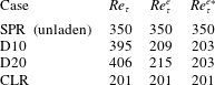
Table 3 presents the mean wall shear, expressed in terms of the friction Reynolds number
 $Re_{\unicode[STIX]{x1D70F}}=u_{\unicode[STIX]{x1D70F}}h/\unicode[STIX]{x1D708}$
from the different simulations considered here. As expected from (3.3) and (3.4), the addition of finite-size neutrally buoyant particles results in an increase in drag with respect to the value of 350 of the single-phase flow, which (when fixing the other governing parameters) increases with increasing particle size. We first note that the smaller the particles, the more the suspension friction Reynolds number
 $Re_{\unicode[STIX]{x1D70F}}^{e}=Re_{\unicode[STIX]{x1D70F}}\unicode[STIX]{x1D708}/\unicode[STIX]{x1D708}^{e}$
approaches the value obtained in the continuum limit, CLR; in other words using an effective viscosity provides a better prediction of the total drag. This is a consequence of the reduced finite-size effects that typically occur near the wall (Costa et al.
Reference Costa, Picano, Brandt and Breugem2016).
Friction Reynolds numbers for the different cases studied.
 $Re_{\unicode[STIX]{x1D70F}}=u_{\unicode[STIX]{x1D70F}}h/\unicode[STIX]{x1D708}$
is the typical friction Reynolds number defined from the wall friction velocity and fluid viscosity,
 $Re_{\unicode[STIX]{x1D70F}}^{e}=Re_{\unicode[STIX]{x1D70F}}\unicode[STIX]{x1D708}/\unicode[STIX]{x1D708}^{e}$
is instead defined from the suspension effective viscosity and
 $Re_{\unicode[STIX]{x1D70F}}^{e\ast }=u_{\unicode[STIX]{x1D70F}}(1-\unicode[STIX]{x1D6FF}_{pw}/h)^{1/2}(h-\unicode[STIX]{x1D6FF}_{pw})/\unicode[STIX]{x1D708}^{e}=Re_{\unicode[STIX]{x1D70F}}^{e}(1-\unicode[STIX]{x1D6FF}_{pw}/h)^{3/2}$
is defined from a wall friction velocity and channel height corrected for finite-size effects and the effective suspension viscosity.

Finally, the third column in the table shows the suspension Reynolds number of the HSR,
 $Re_{\unicode[STIX]{x1D70F}}^{e\ast }=Re_{\unicode[STIX]{x1D70F}}^{e}(1-\unicode[STIX]{x1D6FF}_{pw}/h)^{3/2}$
, obtained considering both an effective suspension viscosity and a virtual-wall origin as explained above (with
 $\unicode[STIX]{x1D6FF}_{pw}$
computed with
 $C=1.5$
and
 $\unicode[STIX]{x1D6F7}_{\max }=0.6$
). The friction Reynolds numbers from the interface-resolved simulations are, in this case, equal for both particle sizes and very close to the value of
 $Re_{\unicode[STIX]{x1D70F}}\unicode[STIX]{x1D708}/\unicode[STIX]{x1D708}^{e}$
for the CLR case. This strongly supports the proposed correction for finite-size effects.
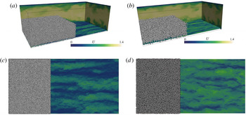
Instantaneous snapshots of the flow for cases D10 (a) and D20 (b). The contours show the magnitude of streamwise velocity (normalized by
 $U_{b}$
) in three mutually perpendicular planes. Particles are illustrated in part of the domain. The bottom plane corresponds to a wall-normal distance of
 $y=1.5D_{p}$
, also shown in a 2D perspective in panels (c) (D10) and (d) (D20).

Figure 1 displays snapshots of the flow for the two laden cases, D10 and D20. Panels (
 $a$
) and (
 $b$
) show planar sections coloured by the streamwise flow velocity, and particle positions only shown for streamwise locations smaller than
 $0.4L_{x}$
and wall-normal distance
 $y<h$
. The bottom plane (also shown in the two planar views (panels
 $c$
and
 $d$
)) corresponds to a wall-normal position
 $y=1.5D_{p}$
, corresponding to approximately
 $y/\unicode[STIX]{x1D6FF}_{v}=15$
and
 $30$
for cases D10 and D20, respectively. The figures show the typical near-wall low-speed streaks found in single-phase wall-bounded turbulence, also present in these suspensions (Picano et al.
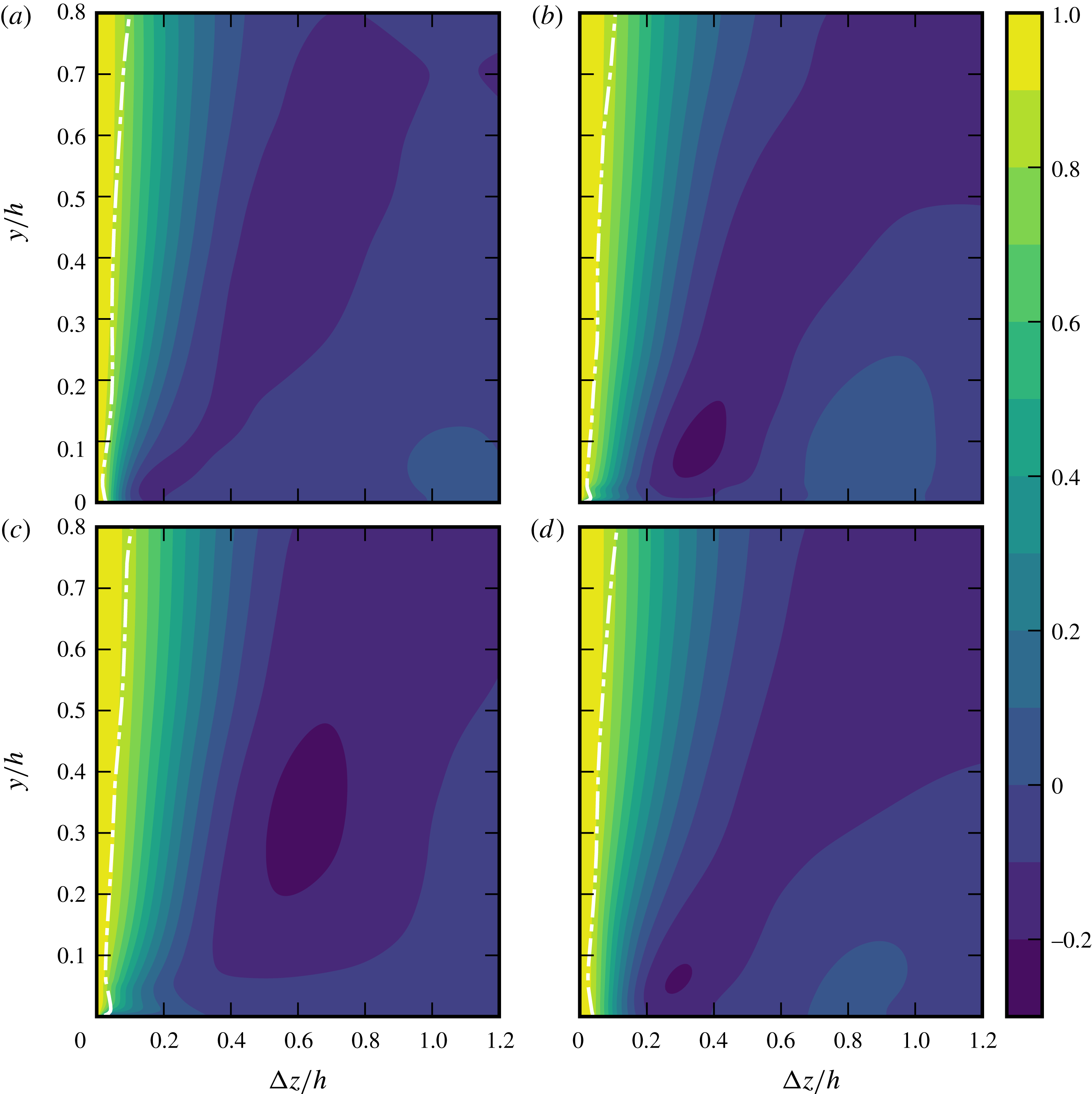
Reference Picano, Breugem and Brandt2015). Differences in velocity contrast between the two cases can be attributed to the choice of a plane at wall-normal distance that scales with the particle diameter, meaning that, in viscous units, the plane corresponding to case D10 is closer to the wall. However, in both cases the maximum streak amplitude is achieved at relatively larger wall-normal distances than what is expected for single-phase flows, as illustrated in figure 2.
This figure depicts contours of autocorrelations of the streamwise suspension velocity (i.e. computed from the fluid flow field with rigid-body motion inside the particles)
 $R_{uu}^{z}(y,\unicode[STIX]{x0394}z)\equiv \langle u^{\prime }(y,z)u^{\prime }(y,z+\unicode[STIX]{x0394}z)\rangle /\langle {u^{\prime }}^{2}(y)\rangle$
, averaged in time and in the streamwise direction for different spanwise separations. Panels (b) and (c) show the results for the interface-resolved simulations D10 and D20. Clearly the near-wall minima – footprint of the low- and high-speed streaks (Kim, Moin & Moser Reference Kim, Moin and Moser1987), and near-wall property that should scale in inner units – are shifted upwards, and the larger the particles are, the larger this shift is.
Figure 2 also shows that the smaller the particles are, the closer the suspension dynamics resemble the continuum limit, CLR. This can be seen when comparing panel (d), corresponding to the continuum limit CLR to panels (b) – D10 and (c) – D20. There is a clear qualitative discrepancy between the CLR and the bigger particles (D20), contrasting with a significant quantitative agreement between CLR and the case with small particles (D10). For case D20, the wall-normal minimum is located at such a large distance to the wall (
 ${\approx}0.3h$
) that inner-to-outer scale separation is compromised. Also, the autocorrelations for the interface-resolved cases show a non-monotonic trend at wall-normal distances
 $y\lesssim D_{p}$
, where the autocorrelation (for fixed
 $y$
) reaches a local maximum close to the wall. This can be even better observed from the profile of the integral length scale
 $L_{xz}=\int _{-L_{z}/2}^{+L_{z}/2}R_{uu}^{z}\,\text{d}(\unicode[STIX]{x0394}z)$
, indicated by the dashed lines in the figure. This confirms that the flow dynamics in this region is qualitatively different from what a simple continuum rheological description would predict.
Autocorrelations of streamwise velocity
 $R_{uu}^{z}$
as a function of the wall-normal distance,
 $y$
, for spanwise separation distances
 $\unicode[STIX]{x0394}z$
(both scaled with
 $h$
) for cases SPR (a), D10 (b), D20 (c) and CLR (d). The dashed lines denote the profile of integral scale
 $L_{xz}(y)$
.

3.2 Flow dynamics near the particle–wall layer (PWL)
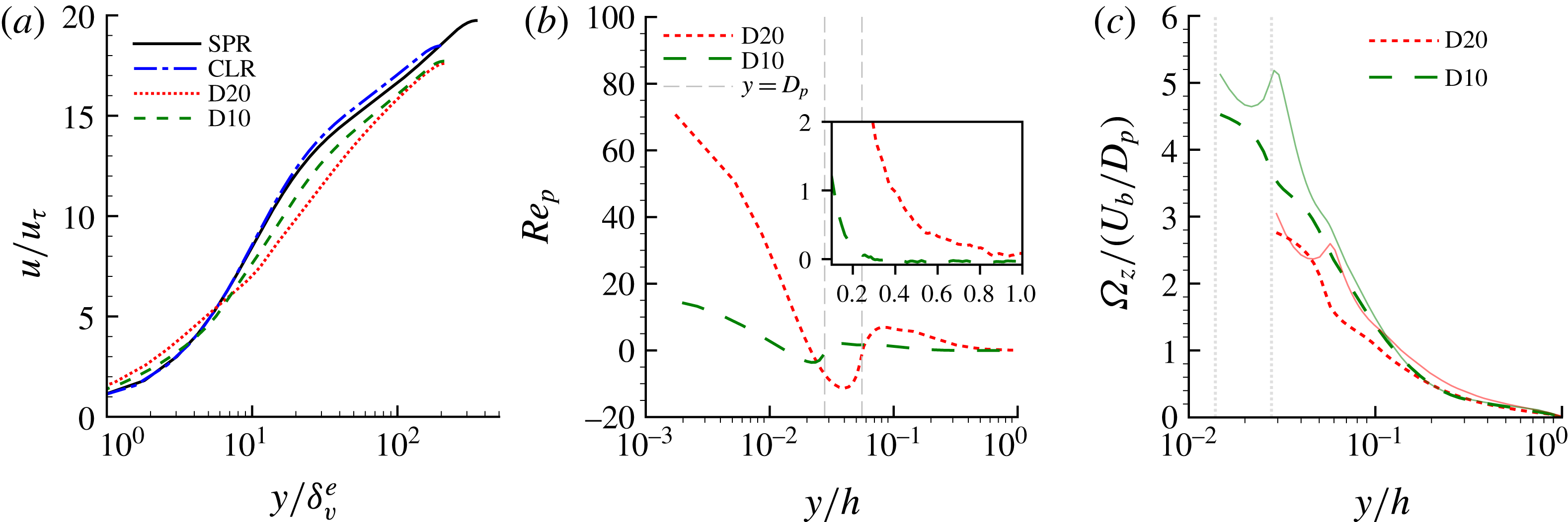
(a) Mean streamwise (inner-scaled) fluid velocity and (b) profile of particle Reynolds number based on the (apparent) particle-to-fluid slip velocity
 $Re_{p}=(u_{p}-u_{f})D_{p}/\unicode[STIX]{x1D708}$
. Vertical dashed lines indicate the wall-normal distance corresponding to one particle diameter. The inset shows the same quantities, but with a linear–linear scale, to highlight the differences in particle Reynolds number in the bulk. Note that both translation and rotation are accounted for when computing
 $u_{p}$
. (c) Fluid and particle angular velocity versus the outer-scaled wall-normal distance. The solid lines depict the fluid velocity, and the vertical dotted lines denote the wall-normal distance corresponding to
 $y=R_{p}$
for both cases.

Next we investigate in more detail the flow dynamics near the particle–wall layer.
Panel (a) of figure 3 depicts the mean streamwise fluid velocity in inner units. Note that the viscous wall unit used for inner scaling is defined, for consistency, with the effective suspension viscosity at the same volume fraction, as we are ultimately interested in the deviations of the flow dynamics from the continuum limit. For wall-normal distances
 $y\gtrsim 10\unicode[STIX]{x1D6FF}_{v}^{e}$
, the profile for the case D10 (smaller particles) clearly shows a logarithmic scaling, with a von Kármán constant
 $\unicode[STIX]{x1D705}=0.36$
. On the other hand, case D20 does not show a clear logarithmic region because of the larger extent of the PWL (Costa et al.
Reference Costa, Picano, Brandt and Breugem2016).
Panel (b) of figure 3 presents the difference between the fluid- and solid-phase velocity profiles, expressed in terms of a particle Reynolds number
 $Re_{p}=(u_{p}-u_{f})D_{p}/\unicode[STIX]{x1D708}$
. Profiles pertaining to the solid phase are obtained by averaging over the rigid-body motion of the particles. Two regions can be clearly distinguished in the figure, roughly separated by the line marking the wall-normal distance
 $y=D_{p}$
. For
 $y\gtrsim D_{p}$
, the difference between the velocity of the two phases is small, whereas the profiles clearly deviate for wall-normal distances
 $y\lesssim D_{p}$
, reaching the highest (apparent) particle-to-fluid slip velocity at the wall. This is a signature of particle layering due to the kinematic constraint that the wall imposes on the particles. Particles flowing at the wall acquire most of their linear momentum at wall-normal distances higher than their radius and this is transported uniformly throughout their volume. Conversely, the fluid momentum must vanish at the wall. Notably, Figure 3(b) shows (see also its inset) that the particle Reynolds number in the bulk is virtually zero for case D10, while it still assumes values of
 $O(1)$
for case D20. This evidence of finite particle inertia in the bulk can result in inertial-shear-thickening effects (see Picano et al.
Reference Picano, Breugem, Mitra and Brandt2013). We will come back to this when the dynamics of the homogeneous suspension region are discussed. Note that in this figure both the effect of particle translation and rotation is accounted for. To discern the effect of rotation, panel (c) of figure 3 compares the profile of particle and fluid angular velocity for the two cases. A similar trend is observed: larger deviations with respect to the fluid profile are found for larger particles, and the highest discrepancy between fluid and particle statistics occurs close to the wall.
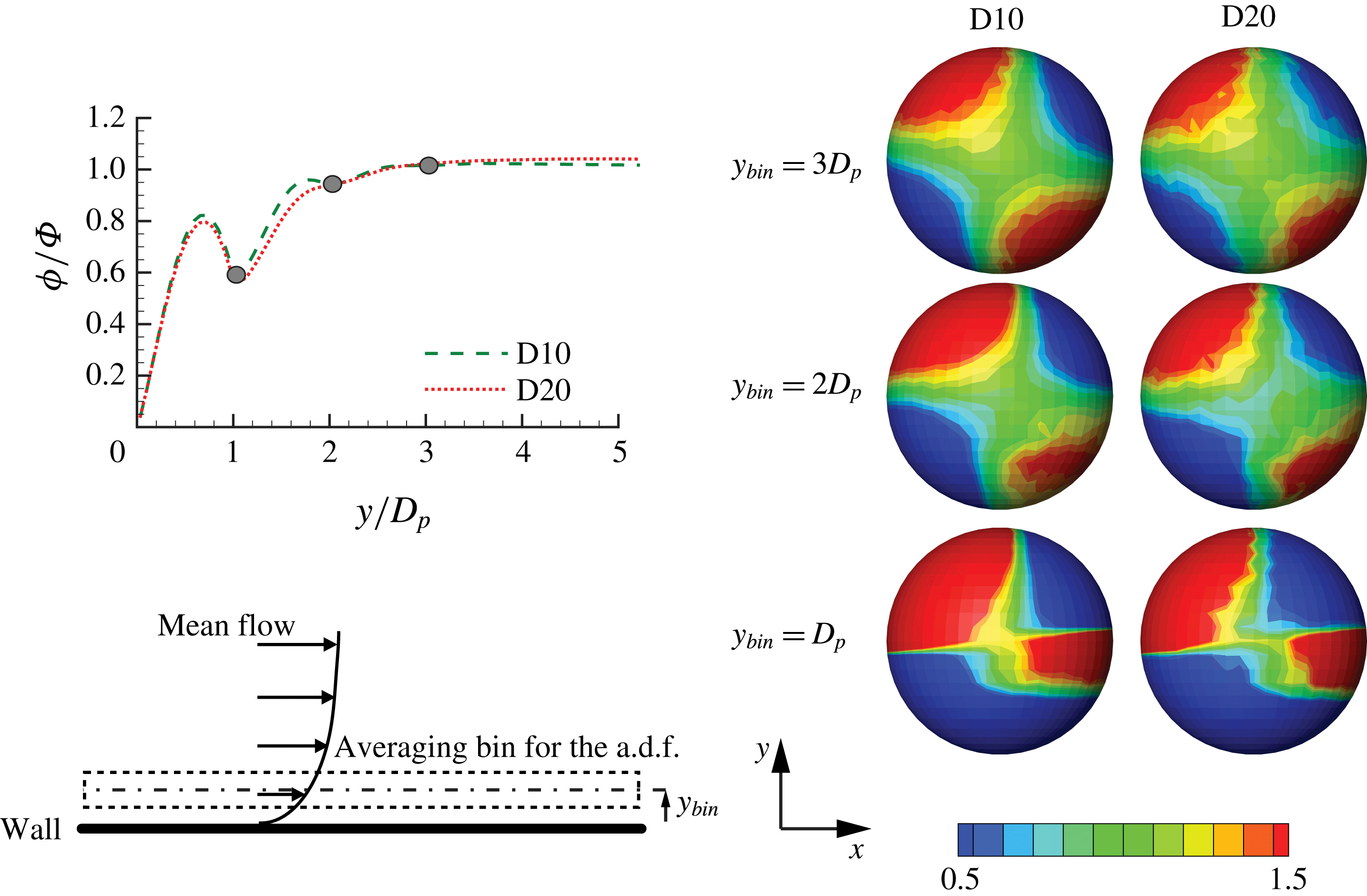
The particle near-wall layer impacts the scale separation on which the scaling laws for mean velocity are based. It is therefore interesting to understand how the near-wall inhomogeneity affects the particle structure, and how far this inhomogeneity extends in the wall-normal direction. We can quantify this through the angular distribution function at contact (a.d.f.). The a.d.f. measures the probability of finding a particle pair at a fixed distance
 $r$
, as a function of the polar (
 $\unicode[STIX]{x1D703}$
) and azimuthal (
 $\unicode[STIX]{x1D711}$
) angles, normalized by the values of a random particle distribution. Formally,
 $$\begin{eqnarray}g(\unicode[STIX]{x1D703},\unicode[STIX]{x1D711})=\frac{1}{r^{2}\sin (\unicode[STIX]{x1D703})}\frac{\text{d}^{2}N_{\unicode[STIX]{x1D703},\unicode[STIX]{x1D711}}}{\text{d}\unicode[STIX]{x1D703}\text{d}\unicode[STIX]{x1D711}}\frac{1}{n_{0}};\quad n_{0}=\frac{N(N-1)}{2V},\end{eqnarray}$$
where
 $N_{\unicode[STIX]{x1D703},\unicode[STIX]{x1D711}}$
denotes the number of particles on a segment of a spherical surface of radius
 $r=D_{p}/2$
, and polar and azimuthal angles within the ranges
 $\unicode[STIX]{x1D703}^{\prime }\in [0,\unicode[STIX]{x1D703}]$
and
 $\unicode[STIX]{x1D711}^{\prime }\in [0,\unicode[STIX]{x1D711}]$
. The a.d.f. is computed from the simulation data using bins with wall-normal extent
 $D_{p}$
, centred at
 $y_{bin}/D_{p}=1$
,
 $2$
and
 $3$
, i.e. at the same wall-normal distance if scaled with the particle size (see the bottom-left corner of figure 4).
Projection onto the
 $x$
–
 $y$
plane of the angular distribution function at contact for simulation D10 and D20. Statistics are obtained within wall-normal slots of size
 $D_{p}$
, centred at
 $y/D_{p}=$
 $1$
,
 $2$
and
 $3$
(flow is from right to left). The curves on the left are the profiles of the mean local volume fraction,
 $\unicode[STIX]{x1D719}/\unicode[STIX]{x1D6F7}$
versus the wall-normal distance
 $y/D_{p}$
, with the markers denoting the locations where the a.d.f. are sampled. These profiles are uniform for
 $y/D_{p}>5$
(Costa et al.
Reference Costa, Picano, Brandt and Breugem2016). The averaging procedure is illustrated on the bottom-left corner.

The projection of the a.d.f. onto the
 $x$
–
 $y$
plane is displayed in figure 4 for the two cases under investigation. For a suspension in homogeneous shear, the particles tend to be preferentially attracted towards each other when located in a compression region (negative local strain) and reciprocally repelled from each other when located in a stretching region (Morris Reference Morris2009). This results in a distribution with two planes of symmetry: two regions of higher clustering in the
 $xy>0$
quadrants and two of lower accumulation in the
 $xy<0$
quadrants. The inhomogeneity introduced by the wall, bounding the particle trajectories, induces a deviation from this picture. The wall effect vanishes for wall-normal distances
 $y/D_{p}\gtrsim 3$
for both simulations. Interestingly, both a.d.f. agree quantitatively. As the distance from the wall is normalized by the particle diameter, for fixed volume fraction, the wall inhomogeneity affects the particle dynamics at distances proportional to
 $D_{p}$
, despite the different local behaviour (different wall-normal location in viscous units) of the suspending fluid.
The local volume fraction profile also presented in figure 4 illustrates that the near-wall inhomogeneity vanishes above
 $y\sim 4D_{p}$
. For higher wall-normal distances this profile is uniform (Costa et al.
Reference Costa, Picano, Brandt and Breugem2016). It is interesting to note that a denser near-wall layer was existing at lower Reynolds numbers for the same volume fraction (see, for example, Picano et al. (Reference Picano, Breugem and Brandt2015), Wang et al. (Reference Wang, Peng, Guo and Yu2016), Yu et al. (Reference Yu, Vinkovic and Buffat2016)). This decrease of layering is attributed to the stronger mixing in this flow due to a higher Reynolds number.
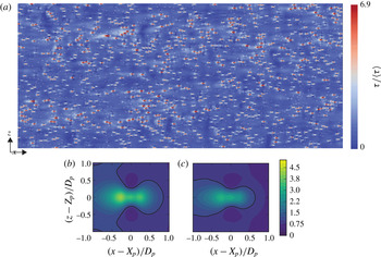
Contours of wall shear stresses (normalized with the corresponding mean value) for case D20 (a). Mean wall shear conditioned to the locations of the near-wall particles and normalized with the mean wall shear for cases D10 (b) and D20 (c). The data are extracted from the average of the top and bottom walls for one temporal realization.

Let us now investigate the influence of the particle–wall layer on the distribution of wall shear stress. To this end, we report in figure 5 contours of the instantaneous wall shear for the case D20, together with the particle positions close to the wall (shown with transparency). The data reveal a strong correlation between regions of high shear and the particle location. This can explain the increase in drag with respect to predictions from the continuum limit: high particle-to-fluid apparent slip velocity close to the wall corresponds locally to events of high wall shear stress, which are not present in the ‘equivalent’ single-phase flow with a modified suspension viscosity. Panels (b) and (c) of the same figure show the mean wall shear conditioned to the particle positions. Results for small and large particles show a similar qualitative behaviour: the shear is higher than the mean around the particles, except close to the surface of the particle, in the spanwise direction. This is a consequence of the reduction of streamwise velocity as the fluid moves around the particle. The contours of the shear stress for the smaller particles show a higher local increase in shear stress, which is, on the other hand, more localized. In fact, the contribution of these hotspots of shear stresses to the total shear (computed from a conditional average of the wall shear stresses in a
 $2D_{p}\times 2D_{p}$
underneath the particle) is the same for both cases, D10 and D20, and quite high:
 $69\,\%$
.
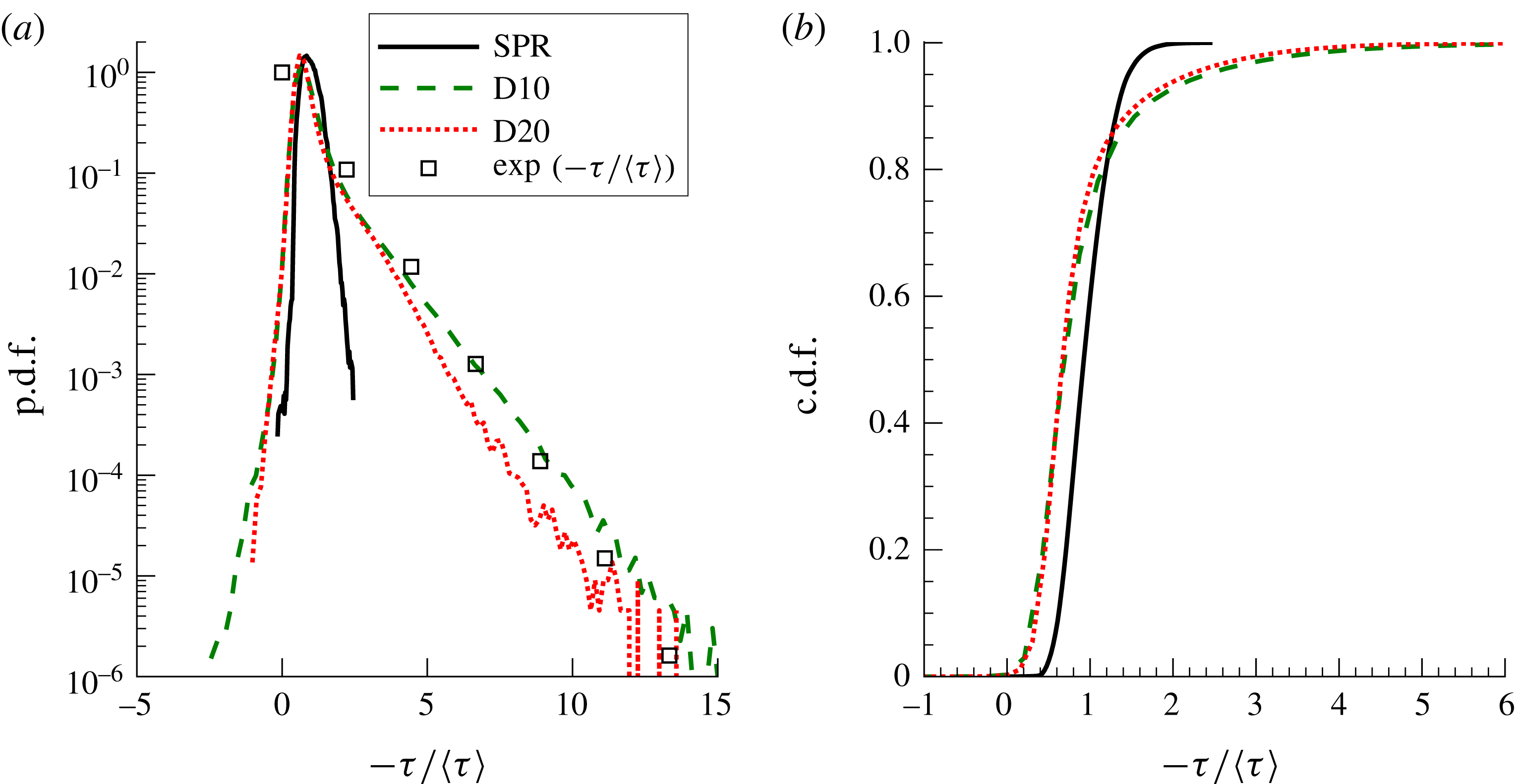
(a) Probability density function and (b) corresponding cumulative distribution function of wall shear stress (normalized with its global mean
 $\unicode[STIX]{x1D70C}u_{\unicode[STIX]{x1D70F}}^{2}$
) for cases D20, D10 and SPR.

The probability density function (p.d.f.) of the shear stress distribution for cases D20, D10 and SPR, presented in figure 6, shows a clear difference between the typical distribution of shear stresses for a single-phase flow, and for the particle-laden cases. In the presence of particles, the tails of the p.d.f. are greatly widened, with very high probability of finding values of the shear stress up to four times the mean value, and likewise for values lower than the mean, including negative events. We note there that it is reported for single-phase flow that
 $\unicode[STIX]{x1D70F}_{w}^{+,rms}=\unicode[STIX]{x1D70F}_{w}^{rms}/\langle \unicode[STIX]{x1D70F}_{w}\rangle \approx 0.4$
and that the p.d.f. typically follows a log-normal distribution (Örlü & Schlatter Reference Örlü and Schlatter2011). Indeed, we obtained a value of
 $\unicode[STIX]{x1D70F}_{w}^{+,rms}=0.39$
for case SPR, with a p.d.f. well fitted by a log-normal distribution (not shown). The hotspots of high shear cause a striking difference for the laden cases:
 $\unicode[STIX]{x1D70F}_{w}^{+,rms}=1.1$
and
 $1.0$
for cases D10 and D20, respectively. Moreover, the p.d.f. no longer fits a log-normal distribution. The hotspots of high wall shear induce a kink in the p.d.f. for
 $\unicode[STIX]{x1D70F}\gtrsim \langle \unicode[STIX]{x1D70F}\rangle$
, resulting in a clear exponential tail, fitted by
 $\unicode[STIX]{x1D706}\exp (-\unicode[STIX]{x1D706}\unicode[STIX]{x1D70F}/\langle \unicode[STIX]{x1D70F}\rangle )$
with
 $\unicode[STIX]{x1D706}\approx 1$
. Further, case D10 shows a higher probability of extreme events, (which, again, are more localized). The largest values attained by the shear stress, that in single-phase flows do not contribute significantly to the mean shear, account for approximately
 $10\,\%$
of the total in particle-laden channel flows, as shown by the cumulative probability distribution function (c.d.f.) displayed in panel (b).
The results presented so far shed light on the relation between the wall slip velocity
 $U_{pw}=u_{p}(y=0)$
and the wall friction
 $u_{\unicode[STIX]{x1D70F}}$
(recall figure 3
 $b$
). Assuming that (1) the average shear in the hotspots matches the average wall shear and (2) the particles impose a mean shear that scales with
 $U_{pw}/D_{p}$
over an area
 $D_{p}L_{w}$
(
 $L_{w}$
being the streamwise extent of the hotspot, which as seen in figure 5 is significantly larger than
 $D_{p}$
), we can write
 $$\begin{eqnarray}N_{pw}D_{p}L_{w}\unicode[STIX]{x1D707}\frac{U_{pw}}{D_{p}}=\unicode[STIX]{x1D70C}u_{\unicode[STIX]{x1D70F}}^{2}L_{x}L_{z},\end{eqnarray}$$
with
 $N_{pw}$
the number of particles in this layer. Further noting that
 $N_{pw}D_{p}^{3}/(D_{p}L_{x}L_{z})\sim \unicode[STIX]{x1D6F7}$
, we have
 $$\begin{eqnarray}\unicode[STIX]{x1D6F7}\frac{L_{w}}{D_{p}}\frac{U_{pw}}{D_{p}}\sim \frac{u_{\unicode[STIX]{x1D70F}}^{2}}{\unicode[STIX]{x1D708}},\end{eqnarray}$$
and finally, assuming that
 $L_{w}/D_{p}$
scales as the mean free path in a two-dimensional layer of particles, i.e.,
 $\propto \unicode[STIX]{x1D6F7}^{-1/2}$
, we obtain
 $$\begin{eqnarray}\frac{U_{pw}}{u_{\unicode[STIX]{x1D70F}}}=C_{pw}Re_{\unicode[STIX]{x1D70F}}^{p}\unicode[STIX]{x1D6F7}^{-1/2},\end{eqnarray}$$
with
 $Re_{\unicode[STIX]{x1D70F}}^{p}=u_{\unicode[STIX]{x1D70F}}D_{p}/\unicode[STIX]{x1D708}$
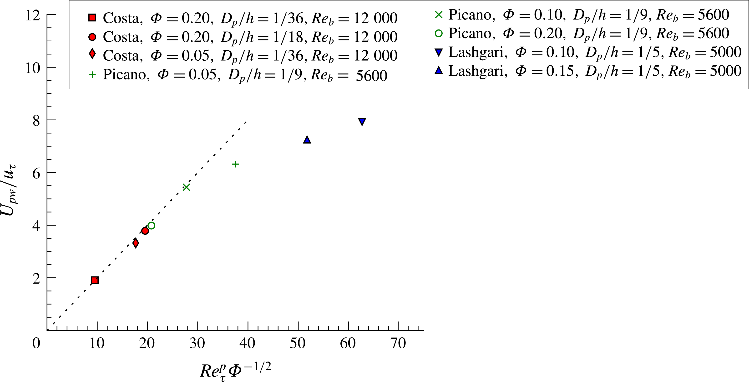
a particle friction Reynolds number. The data in figure 7, including previous cases in literature, confirm the validity of this relation with
 $C_{pw}\approx 0.2$
. The data points that do not follow the predicted scaling correspond to very large particles (
 $h/D_{p}=5$
), for which the influence of the outer scales on the near-wall particle dynamics compromises the first assumption above, and to low volume fractions.
Particle-to-fluid slip velocity
 $U_{pw}$
normalized with the wall friction velocity
 $u_{\unicode[STIX]{x1D70F}}$
versus
 $Re_{\unicode[STIX]{x1D70F}}^{p}\unicode[STIX]{x1D6F7}^{-1/2}$
(see definition in the text). To support the validity of the proposed scaling, data from Picano et al. (Reference Picano, Breugem and Brandt2015) and Lashgari et al. (Reference Lashgari, Picano, Breugem and Brandt2014) are also included.

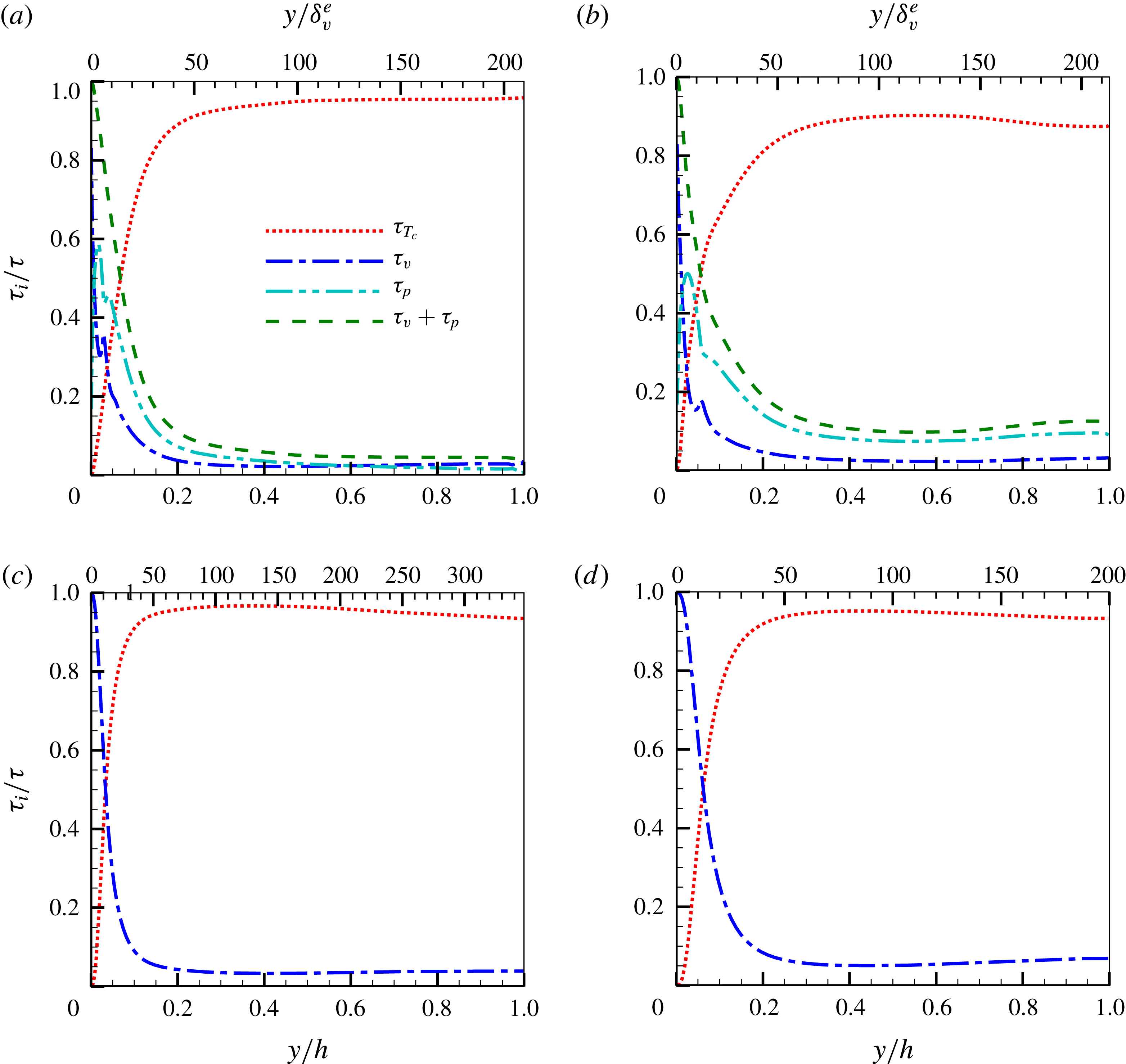
Stress contributions
 $\unicode[STIX]{x1D70F}_{i}(y)/(u_{\unicode[STIX]{x1D70F}}^{2}(1-y/h))$
for the different cases D10 (a), D20 (b), SPR (c) and CLR (d), see equation (3.9).
 $\unicode[STIX]{x1D70F}_{T_{c}}=\unicode[STIX]{x1D70F}_{T_{f}}+\unicode[STIX]{x1D70F}_{T_{p}}$
denotes the contribution of the Reynolds stresses of the combined phase.

3.3 Homogeneous suspension region (HSR)
The contribution of the different stresses to the suspension streamwise momentum transport (i.e. the stress budget) can be derived from volume- and ensemble-averaging the mixture streamwise momentum equation (see Marchioro, Tanksley & Prosperetti Reference Marchioro, Tanksley and Prosperetti1999; Picano et al. Reference Picano, Breugem and Brandt2015). It reads for plane channel flow
 $$\begin{eqnarray}\langle \unicode[STIX]{x1D70F}\rangle =u_{\unicode[STIX]{x1D70F}}^{2}\left(1-\frac{y}{h}\right)=\underbrace{(1-\unicode[STIX]{x1D719})\langle -u_{f}^{\prime }v_{f}^{\prime }\rangle }_{\unicode[STIX]{x1D70F}_{T_{f}}}+\underbrace{(1-\unicode[STIX]{x1D719})\unicode[STIX]{x1D708}\frac{\text{d}U_{f}}{\text{d}y}}_{\unicode[STIX]{x1D70F}_{v}}+\underbrace{\unicode[STIX]{x1D719}\langle -u_{p}^{\prime }v_{p}^{\prime }\rangle }_{\unicode[STIX]{x1D70F}_{T_{p}}}+\unicode[STIX]{x1D70F}_{p},\end{eqnarray}$$
where the terms on the right-hand side denote the fluid Reynolds stresses
 $\unicode[STIX]{x1D70F}_{T_{f}}$
, the viscous stresses
 $\unicode[STIX]{x1D70F}_{v}$
, the particle Reynolds stresses
 $\unicode[STIX]{x1D70F}_{T_{p}}$
, and the particle stresses
 $\unicode[STIX]{x1D70F}_{p}$
, the latter related to the stresslet, moment of the material acceleration acting on a particle and interparticle collisions (Guazzelli & Morris Reference Guazzelli and Morris2011); in the expression above,
 $\unicode[STIX]{x1D719}$
denotes the mean local solid volume fraction. The wall-normal profiles of the different contributions to the total stress (obtained dividing (3.9) by
 $u_{\unicode[STIX]{x1D70F}}^{2}(1-y/h)$
) are reported in figure 8. As also observed in Lashgari et al. (Reference Lashgari, Picano, Breugem and Brandt2016, Reference Lashgari, Picano, Breugem and Brandt2014), Picano et al. (Reference Picano, Breugem and Brandt2015) the profiles of particle stresses reach a maximum at
 $y=D_{p}/2$
, at the location of the local maximum of the profiles of the local volume fraction (see figure 4), followed by a minimum at
 $y\sim 2D_{p}$
. The Reynolds stresses are relatively small in this region, and therefore the local maximum/minimum of the particle stresses is compensated by a local minimum/maximum of the viscous shear stresses. This is caused by the strong shear that the first layer of particles, flowing with significant slip velocity, imposes on the fluid above it. Further away from the wall, the profiles follow a trend that resembles the one of the shear-stress profile, suggesting a linear (Newtonian) scaling of the particle stresses with the shear rate.
The deviation from the continuum limit (CLR) can be examined by comparing the sum of the particle and viscous stresses to the profile of viscous stresses in panel (d) of figure 8 (note that an effective viscosity incorporates the effects of both viscous and particle stresses). As expected, the case with smaller particles is much closer to this continuum limit than the case with larger particles (see also Costa et al.
Reference Costa, Picano, Brandt and Breugem2016). For the latter, while the profile pertaining to the viscous contribution in the bulk is still close to the one of case D10, the particle stress contribution is much larger. This difference can be attributed to the inertial-shear-thickening mechanism due to excluded volume effects proposed in Picano et al. (Reference Picano, Breugem, Mitra and Brandt2013), as the particle Reynolds number based on the particle slip velocity for case D20 is much larger (recall figure 3
b). We should stress here the importance of defining the viscous wall unit from the effective suspension viscosity: if the profiles of cases D10 and D20 were to be compared to CLR using the classical inner scaling (where the fluid viscosity and wall friction velocity are used to scale the wall-normal distance) these would not match, as the abscissa on the upper axis
 $y/\unicode[STIX]{x1D6FF}_{v}^{e}$
would have to be multiplied by
 $\unicode[STIX]{x1D708}^{e}/\unicode[STIX]{x1D708}=1.89$
in panels (a) and (b) of figure 8.
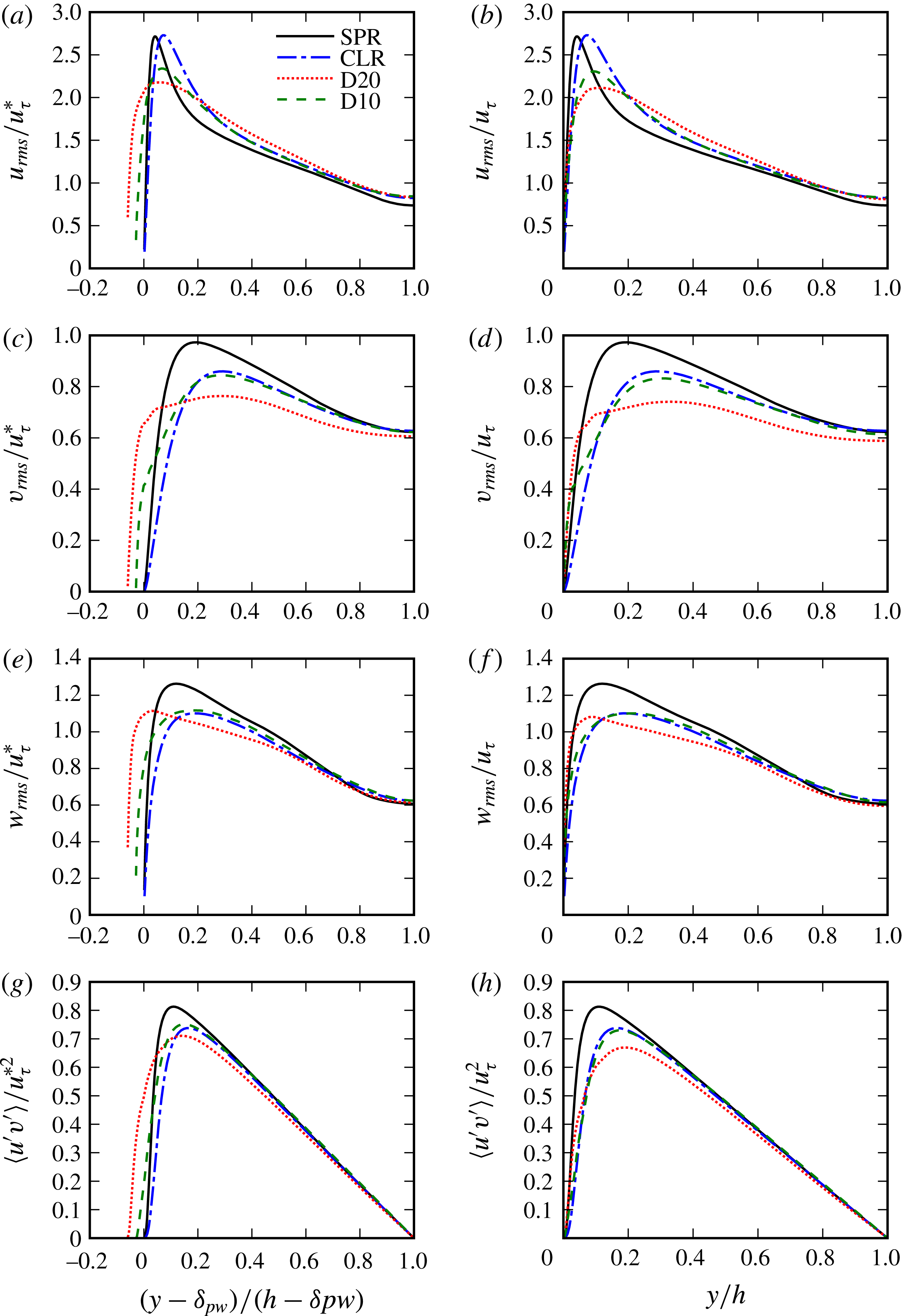
As for the other quantities presented so far, we expect the second-order Eulerian statistics for the laden cases to approach those of CLR with decreasing particle size. These are shown in figure 9, where we depict the profiles of the root mean square (r.m.s.) of the fluctuating fluid velocity and Reynolds stresses from the different simulations. When comparing to the single-phase flow statistics we also observe, as reported in Picano et al. (Reference Picano, Breugem and Brandt2015), that the fluctuating fluid velocity close to the wall is enhanced by the presence of the particles.
Let us take one step further and test the scaling arguments of Costa et al. (Reference Costa, Picano, Brandt and Breugem2016) for the second-order statistics. These can be compared directly to the case CLR, as it is meant to be the same flow, finite-size effects aside. We therefore correct the wall-normal distance for the presence of the particle–wall layer through a virtual- wall origin,
 $\unicode[STIX]{x1D6FF}_{pw}$
, and correct velocity scale for inner scaling,
 $u_{\unicode[STIX]{x1D70F}}^{\ast }=u_{\unicode[STIX]{x1D70F}}(1-\unicode[STIX]{x1D6FF}_{pw}/h)^{1/2}$
(panels a,c,e,g in figure 9). The magnitude of near-wall peaks in streamwise velocity r.m.s., typically located at
 $y=12\unicode[STIX]{x1D6FF}_{v}\lesssim D_{p}$
, are not recovered in the interface-resolved simulations. Despite this, away from the wall (where the dynamics is only weakly affected by the particle–wall layer due to sufficient scale separation) the profiles show good agreement. Particularly, the profiles pertaining to case D10 show a remarkable collapse over the entire outer region for all three components of the velocity r.m.s. and Reynolds stresses, even without correction. The same cannot be safely stated for the case with larger particles (D20) where finite-size effects, also present away from the particle–wall layer, have an influence on the statistics in the bulk of the flow. Despite these small deviations for case D20, it is clear that, away from the wall, the second-order statistics are described with good approximation by those of a Newtonian fluid with an effective suspension viscosity.
Profile of r.m.s. of fluctuating streamwise, spanwise and wall-normal fluid velocity from the different simulations. Classical scaling is used in panels (b,d,f,h), whereas the scaling laws of Costa et al. (Reference Costa, Picano, Brandt and Breugem2016) are used in panels (a,c,e,g).

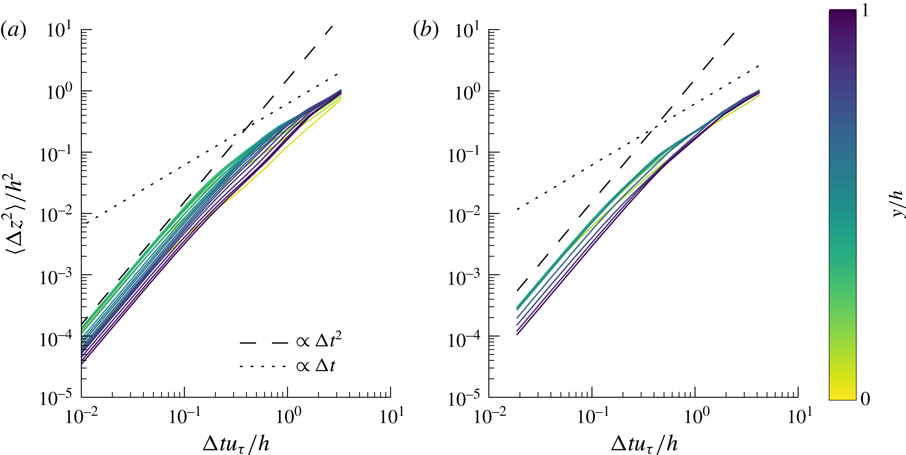
Single-particle mean-square spanwise displacement
 $\langle \unicode[STIX]{x0394}z_{1}^{2}\rangle (\unicode[STIX]{x0394}t,y)$
normalized with the half channel height
 $h^{2}$
, for cases (a) D10 and (b) D20 versus time in units of the integral time scale
 $h/u_{\unicode[STIX]{x1D70F}}$
. The colours indicate different wall-normal distances.

3.4 Particle dynamics
Analysing the mean flow solely in an Eulerian framework does not give direct insights on the dynamics of individual particles. To better understand the particle dynamics, we further explore the DNS dataset by computing Lagrangian statistics. We first focus on the evolution of the single-point mean-square displacement of particles in the spanwise direction to prevent biases due to statistical inhomogeneity in the wall-normal, and non-zero mean flow in the streamwise direction (see also Lashgari et al. Reference Lashgari, Picano, Breugem and Brandt2016). This is defined as
 $$\begin{eqnarray}\langle \unicode[STIX]{x0394}z_{1}^{2}\rangle (\unicode[STIX]{x0394}t,y)=\langle \left(z(t+\unicode[STIX]{x0394}t)-z(t)\right)^{2}\rangle ,\end{eqnarray}$$
where
 $\langle \rangle$
denotes the time average over all particles located in a bin centred at a wall-normal position
 $y$
at time
 $t$
and wall-normal extent
 $D_{p}$
. This observable is displayed in figure 10 versus time in units of a characteristic integral scale of the turbulent fluid motion,
 $h/u_{\unicode[STIX]{x1D70F}}$
. One can distinguish two well-known regimes: the ballistic regime, where the high temporal correlation results in a mean-square displacement
 $\langle \unicode[STIX]{x0394}z_{1}^{2}\rangle \propto \unicode[STIX]{x0394}t^{2}$
, and the diffusive regime, where the motion decorrelates from the initial sampling instant and
 $\langle \unicode[STIX]{x0394}z_{1}^{2}\rangle \propto \unicode[STIX]{x0394}t$
(see, for example, Sierou & Brady (Reference Sierou and Brady2004)). In the ballistic regime, particles reach the fastest dispersion at the distance from the wall corresponding to the peak in particle velocity r.m.s. (see figure 9). The diffusion coefficient (slope of the profile in the diffusive regime) is nearly the same for the both cases, away from the wall. Two main mechanisms are responsible for the spanwise particle displacements and the subsequent self-diffusion: (1) short-range interparticle interactions and (2) interactions with turbulent structures of dimension larger than the particle size. One can picture a sequence of these events as successive random-walk steps during the particle motion. Indeed, Lashgari et al. (Reference Lashgari, Picano, Breugem and Brandt2016) observed in the turbulent regime an increase of the diffusion coefficient with increasing Reynolds number for fixed volume fraction, and a milder increase with increasing volume fraction at fixed Reynolds number. The smaller diffusion coefficients observed near the wall can therefore be explained by the constraint that the wall confinement imposes on the particle motion, and by the reduction of the characteristic turbulent integral scale, estimated as
 $l_{m}(y)\sim \min (\unicode[STIX]{x1D705}y,0.1h)$
note: I changed to
 $l_{m}(y)$
, with
 $l_{m}$
being a mixing length (Pope Reference Pope2001). The turbulent length scales are hindered up to a point where
 $l_{m}\sim D_{p}$
, the value below which turbulent fluctuations have a weak influence on the particle kinematics. Despite the relatively small particle inertia, the temporal filtering due to the higher response time of the larger particles (Hinze Reference Hinze1975) can also cause a decrease in diffusion coefficient. However, we expect the latter effect to be milder, as increasing particle inertia through an increased mass density (while fixing the other governing parameters) has a small influence on spanwise particle dispersion, as shown in Fornari et al. (Reference Fornari, Formenti, Picano and Brandt2016a
).
The diffusion coefficient is larger for the flow with smaller particles (D10), even though the collision probability is larger for the largest particles (as suggested by the asymptotic limit of vanishing particle size at fixed volume fraction, and will be confirmed later). We can therefore conclude that, at the volume fraction under consideration here, the turbulent fluid motion is the main source of self-diffusion and, consequently, larger particles result in slower dispersion. Note also that the diffusive regime is reached away from the wall at times
 $\unicode[STIX]{x0394}t=O(h/u_{\unicode[STIX]{x1D70F}})$
of the same order as the turnover time of large eddies in the bulk, consistently with this observation.
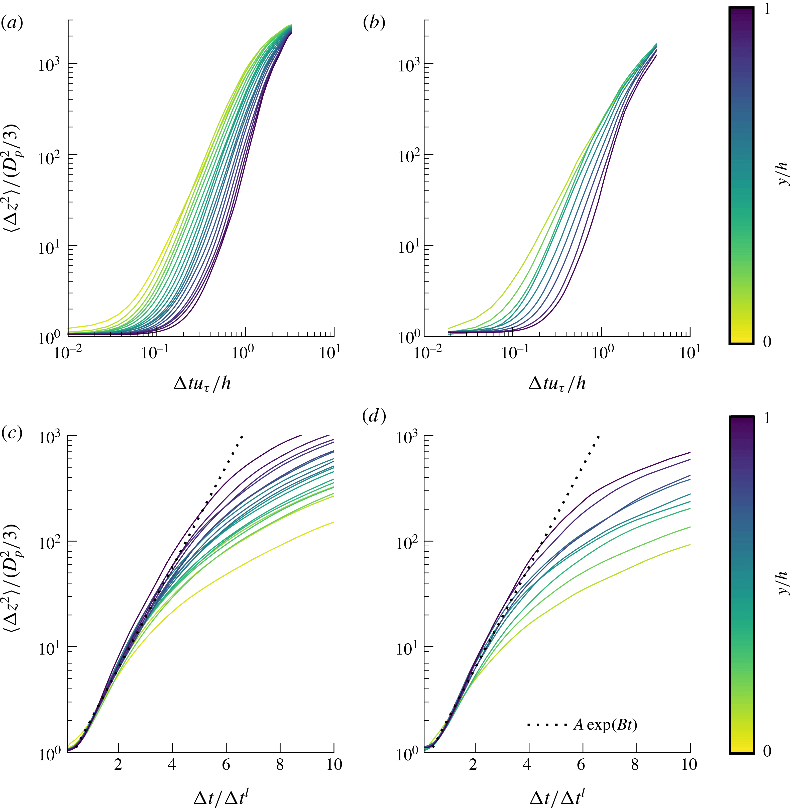
Further insight into the particle dynamics can be gained by examining the pair-dispersion statistics. The two-point mean spanwise square displacement is displayed in figure 11 for two particles at contact at
 $t=t_{0}$
,
 $$\begin{eqnarray}\langle \unicode[STIX]{x0394}z_{2}^{2}\rangle (\unicode[STIX]{x0394}t,y)=\langle \left(\unicode[STIX]{x1D6FF}z(t_{0}+\unicode[STIX]{x0394}t)-\unicode[STIX]{x1D6FF}z(t_{0})\right)^{2}\rangle ,\end{eqnarray}$$
where
 $\unicode[STIX]{x1D6FF}z$
denotes the spanwise interparticle distance and
 $t_{0}$
the instant at which the particles are in contact. For short time scales, lubrication dominates and the particles display a highly correlated motion. The duration of this regime increases with the distance to the wall. This slower relative dispersion is linked to the decreasing relative interparticle velocity towards contact with increasing wall-normal distance, to be quantified later. The large particles, case D20, show faster pair dispersion, also due to higher relative interparticle velocity towards contact: it turns out, as elaborated later when the collisional dynamics is addressed, that this quantity scales with the particle Reynolds number. At later times, the particle dispersion
 $\langle \unicode[STIX]{x0394}z_{2}^{2}\rangle \propto \unicode[STIX]{x0394}t^{\unicode[STIX]{x1D6FC}}$
, with
 $2<\unicode[STIX]{x1D6FC}<3$
. Note that for tracer particles in a homogeneous isotropic turbulent flow
 $\unicode[STIX]{x1D6FC}=3$
for separation distances within the inertial subrange (Salazar & Collins Reference Salazar and Collins2009). For larger separation distances the diffusive limit is recovered.
The mean-square displacement of tracer particles in turbulence with sub-Kolmogorov separation distance (i.e. in the dissipation subrange) grows exponentially in time as the relative particle velocity and the separation are proportional (Batchelor Reference Batchelor1952; Salazar & Collins Reference Salazar and Collins2009): i.e.
 $\langle \unicode[STIX]{x1D6FF}z_{2}^{2}\rangle =\langle \unicode[STIX]{x1D6FF}z_{0}^{2}\rangle \text{e}^{2\unicode[STIX]{x0394}t/t_{c}}$
, where
 $t_{c}$
is a characteristic interparticle response time. Although in the present study
 $D_{p}$
is
 $O(10)$
times larger than the smallest turbulence scale, we observe a clear exponential growth at short times, just after the first highly correlated regime when
 $\langle \unicode[STIX]{x0394}z_{2}^{2}\rangle$
is approximately constant. The time at which this exponential regime sets in corresponds to a mean- square separation of approximately
 $2D_{p}^{2}/3$
. This exponential regime is highlighted in the figure 11(c,d), where the time on the horizontal axis is divided by
 $\unicode[STIX]{x0394}t^{l}=\unicode[STIX]{x0394}t|_{\langle \unicode[STIX]{x0394}z_{2}^{2}\rangle =2D_{p}^{2}/3}$
. This growth is due to a different mechanism than the one of tracer particles, possibly the combination of a uniform shear force (note that under uniform shear
 $\unicode[STIX]{x1D6FF}z$
is proportional to the relative velocity) following a short-range lubrication interaction.
Two-particle mean-square spanwise displacement
 $\langle \unicode[STIX]{x0394}z_{2}^{2}\rangle (\unicode[STIX]{x0394}t,y)$
normalized with the mean initial spanwise square distance at contact
 $D_{p}^{2}/3$
for (a) case D10 and (b) case D20 versus time normalized with the integral time scale
 $h/u_{\unicode[STIX]{x1D70F}}$
. The different lines are colour-coded to indicate the particle–wall-normal distance. Panels (c) and (d) illustrate the initial exponential scaling by plotting the same quantity versus
 $\unicode[STIX]{x0394}t^{l}=\unicode[STIX]{x0394}t|_{\langle \unicode[STIX]{x0394}z_{2}^{2}\rangle =2D_{p}^{2}/3}$
(see discussion in the text). The dotted lines indicate the fitting function
 $A\exp (Bt)$
with
 $A=0.7$
and
 $B=1.1$
.

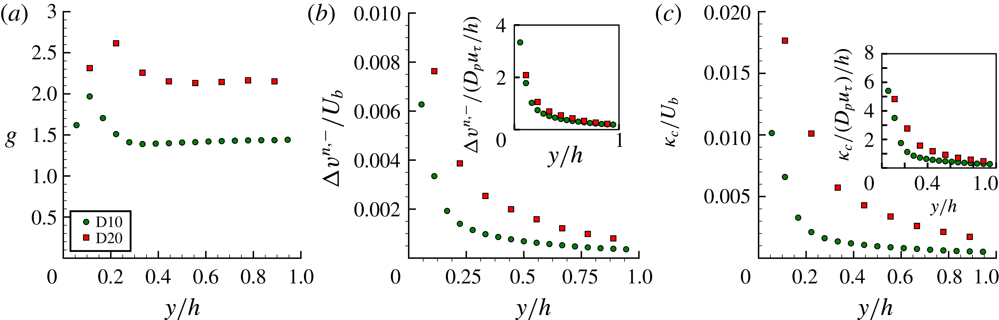
Finally, we investigate the particle collisional dynamics. A collision event takes place when (1) the particles are at sufficiently close distance and (2) their relative velocity drives them towards contact. These two factors are investigated separately. The first by the radial distribution function (rdf), which quantifies the probability of finding a second particle at distance
 $r$
normalized by the probability of a random distribution of particles:
 $$\begin{eqnarray}g(r,y)=\frac{1}{4\unicode[STIX]{x03C0}r^{2}}\frac{\text{d}N_{r}}{\text{d}r}\frac{1}{n_{0}},\end{eqnarray}$$
where
 $N_{r}$
denotes the number of particle pairs in a spherical volume of radius
 $r$
. Thus, if
 $g(r,y)$
assumes values larger than
 $1$
, particles are preferentially sampled. The second observable is the distribution of incoming (i.e. towards contact) relative particle velocity projected in the direction of the line of centres
 $\unicode[STIX]{x0394}v^{n,-}$
, given for two particles
 $i$
,
 $j$
with velocities
 $\boldsymbol{u}_{i/j}$
and positions
 $\boldsymbol{x}_{i/j}$
by
 $$\begin{eqnarray}\unicode[STIX]{x0394}v^{n,-}(r,y)=\max \left\{0,-(\boldsymbol{u}_{j}-\boldsymbol{u}_{i})\boldsymbol{\cdot }\frac{\boldsymbol{x}_{j}-\boldsymbol{x}_{i}}{|\boldsymbol{x}_{j}-\boldsymbol{x}_{i}|}\right\}\text{;}\end{eqnarray}$$
where the
 $\max \{\}$
operator samples the relative velocity towards contact, as the superscript ‘
 $-$
’ suggests. The product of these quantities measures the rate at which particles approach each other. Its value for
 $r=D_{p}$
is the so-called collision kernel,
 $\unicode[STIX]{x1D705}_{c}$
, the probability of a collision event.
As for the dispersion statistics, we take into account the inhomogeneity in the wall-normal direction by averaging in wall-parallel bins with wall-normal extent
 $2D_{p}$
. Figure 12 presents the radial distribution function, negative particle relative velocity and the approach rate at contact
 $r=D_{p}$
.
(a) Radial distribution function
 $g(D_{p})$
at contact, (b) normal relative velocity at contact
 $\unicode[STIX]{x0394}v^{n,-}(D_{p})/U_{b}$
and (c) collision kernel
 $\unicode[STIX]{x1D705}_{c}/U_{b}$
versus the outer-scaled wall-normal distance
 $y/h$
. The insets of panels (b) and (c) show the same quantity scaled with the velocity scale
 $u_{\unicode[STIX]{x1D70F}}D_{p}/h$
, see equation (3.14).

The profile of
 $\unicode[STIX]{x0394}v^{n,-}$
shows that the dominant mechanism driving particles towards each other is shear from particles at different wall-normal locations. Note that the shear rate away from the PWL is similar for both simulations considered (see figure 8 and table 3). Assuming that particles are driven towards each other by shearing a layered arrangement of particles:
 $$\begin{eqnarray}\unicode[STIX]{x0394}v^{n,-}\propto D_{p}\frac{\unicode[STIX]{x2202}u}{\unicode[STIX]{x2202}y}\sim D_{p}\frac{u_{\unicode[STIX]{x1D70F}}}{h},\end{eqnarray}$$
with
 $u_{\unicode[STIX]{x1D70F}}/h$
an estimate of the shear rate in the bulk of the flow. This scaling is tested in the inset of panels (b) and (c) of figure 12, yielding a better agreement of the profiles of
 $\unicode[STIX]{x0394}v^{n,-}$
and
 $\unicode[STIX]{x1D705}_{c}$
, despite the differences in
 $g(D_{p})$
. Note that
 $u_{\unicode[STIX]{x1D70F}}/h$
is approximately the same for both cases (table 3). The higher values of
 $g$
at close distances for case D20 are also compatible with this picture, as larger particles are more prone to be driven towards each other by a shear-induced relative motion.
The mechanism governing energy dissipation during particle collisions can be predicted from the impact Stokes number, which can be computed directly from the mean relative approach velocity close to contact:
 $St=(1/9)\unicode[STIX]{x1D70C}_{p}\unicode[STIX]{x0394}v_{max}^{n,-}D_{p}/\unicode[STIX]{x1D707}$
. The Stokes number corresponding to the maximum value of
 $\unicode[STIX]{x0394}v^{n,-}$
, shown in figure 12(b) (case D20), is
 $St\approx 0.28$
. This average Stokes number is therefore much lower than the critical value of
 $10$
everywhere in the domain, suggesting that the collisional dynamics are governed by short-range hydrodynamic interactions, with strong viscous dissipation and no elastic rebound (see Legendre et al. (Reference Legendre, Zenit, Daniel and Guiraud2006) and Yang & Hunt (Reference Yang and Hunt2006)).
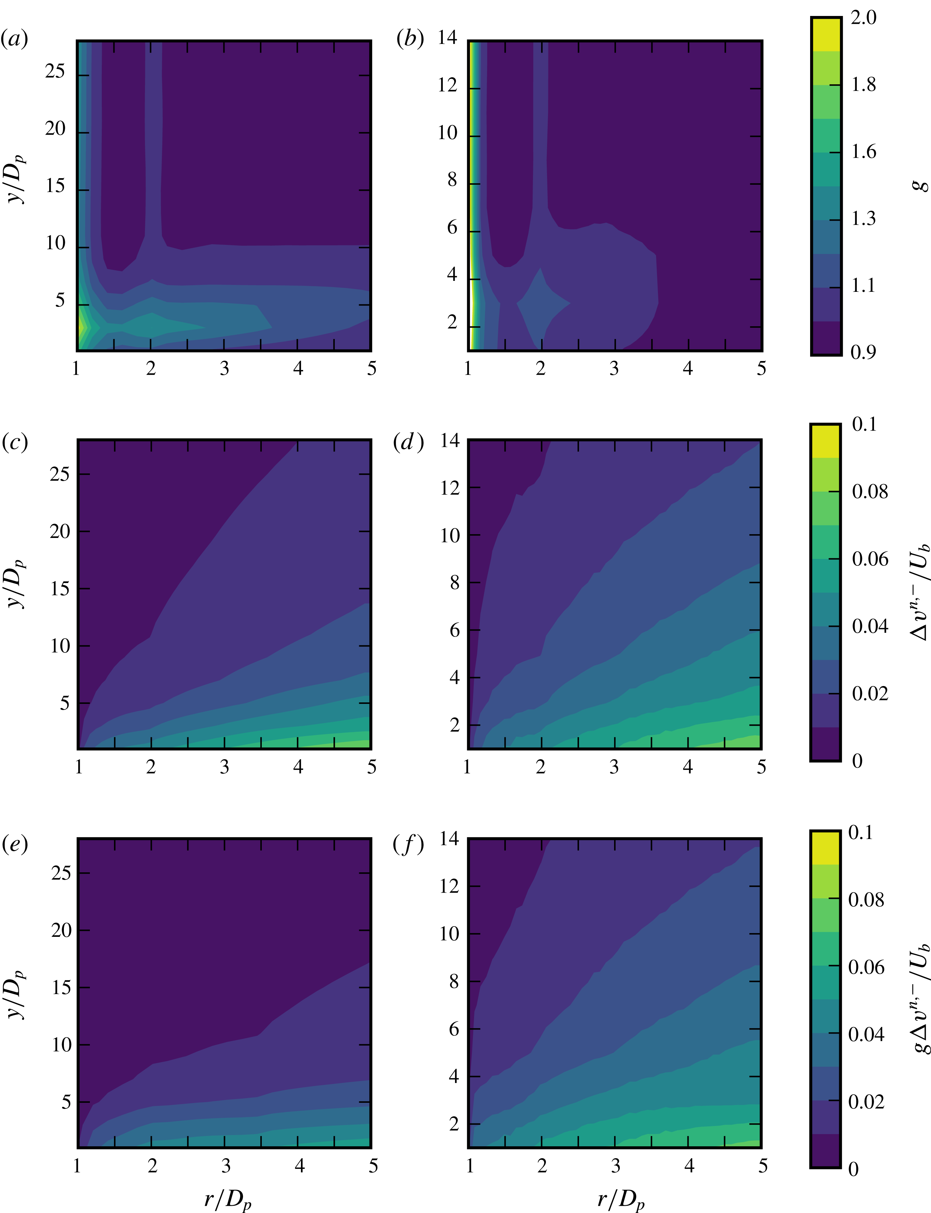
Figure 13 shows contour plots of the same quantities as in figure 12, now as a function of both the separation distance
 $r$
and the wall-normal coordinate
 $y$
. The contours of
 $g$
show that this quantity is weakly dependent on the wall-normal coordinate, with local maxima at
 $r/D_{p}\approx 1$
and
 $2$
, consistent with the presence of statistically significant particle pairs and triplets. It is also interesting to notice that the global maximum of
 $g$
occurs at a finite distance to the wall. Comparing the two simulations, the maximum is located at the same wall-normal distance when scaled with the particle diameter
 $y\sim 3D_{p}$
, in agreement with the observation above that wall-confinement effects are noticeable at distances proportional to the particle diameter (see figure 4). The maxima of
 $g(r)$
correspond therefore to the optimal tradeoff between high shear (driving particles at different wall-normal locations towards each other) and low confinement; indeed further away from the wall, where the mean shear is relatively low,
 $g$
becomes almost independent of
 $y$
. The maxima of
 $g$
close to the wall also suggest that larger particles have higher probability of forming particle pairs, and lower probability of forming triplets.
Figure 13(c,d) displays contours of
 $\unicode[STIX]{x0394}v^{n,-}$
. For fixed separation distance
 $r$
, the average interparticle approaching velocity decreases with the wall-normal distance
 $y$
, which can be explained by a decreasing local shear rate: the lower the shear, the smaller shear-induced differences of the particle relative velocities. Consistently, the variations of
 $\unicode[STIX]{x0394}v^{n,-}$
with
 $y$
are larger close to the wall. The negative relative particle velocity is larger for the largest particles, case D20, over the entire flow, as the scaling suggested in (3.14) predicts. Finally, we report the rate of approach
 $\unicode[STIX]{x0394}v^{n,-}g$
in figure 13(e,f). Clearly, the differences in
 $g$
discussed above induce significant differences in this quantity only close to contact. At larger separation, the behaviour of
 $\unicode[STIX]{x0394}v^{n,-}g$
is dictated by
 $\unicode[STIX]{x0394}v^{n,-}$
.
Contour plot of radial distribution function,
 $g$
(a,b), negative relative velocity
 $\unicode[STIX]{x0394}v^{n,-}/U_{b}$
(c,d), and rate of approach
 $g\unicode[STIX]{x0394}v^{n,-}/U_{b}$
(e,f) for simulation D10 (a,c,e) and D20 (b,d,f) as a function of the wall-normal coordinate (
 $y$
) and separation (
 $r$
) scaled with the particle diameter
 $D_{p}$
.

4 Conclusions and outlook
We performed interface-resolved direct numerical simulations of turbulent channel flow of suspensions of neutrally buoyant spherical particles. Two flow cases are considered, with same Reynolds number and volume fraction, and particle size varied by a factor of two. The simulations are compared to two single-phase reference simulations: (1) the unladen case and (2) the continuum limit of a Newtonian fluid with a viscosity corresponding to the effective viscosity of the suspension under investigation in a laminar shear flow.
As observed in Costa et al. (Reference Costa, Picano, Brandt and Breugem2016), the main finite-size effect in the zero- and first-order Eulerian statistics originate from the near-wall dynamics, in the near-wall particle layer. We show here that the larger the particles are, the further away from the wall the effects of the particle layer are significant. The near-wall inhomogeneity due to the geometrical constraints is felt at distances that scale with the particle size at fixed volume fraction, seemingly independent of the local fluid flow dynamics. This results in a smaller inner-to-outer scale separation for the flow with larger particles, clearly featured in several flow statistics.
Particles at the wall with significant particle-to-fluid slip velocity create hotspots of high local wall shear (on average approximately four times larger than the mean) which contribute significantly to the mean wall stress. These hotspots show higher magnitude of the wall stress for small particles, which are, consistently, more localized. Their contribution to the mean wall shear is nearly the same for both particle sizes considered, approximately
 $70\,\%$
. Also interesting to note is the highly increased probability of local shear stresses lower than the mean, and even negative (i.e., instantaneous flow reversal). These hotspots change considerably the distribution of shear stresses, resulting in a p.d.f. with a wide exponential tail and r.m.s. values,
 $\unicode[STIX]{x1D70F}_{w}^{rms}\approx \unicode[STIX]{x1D70F}_{w}$
, in contrast to what is found in canonical single-phase wall-bounded turbulent flows, where the p.d.f. is well fitted by a log-normal distribution and
 $\unicode[STIX]{x1D70F}_{w}^{rms}\approx 0.4\unicode[STIX]{x1D70F}_{w}$
. To quantify, the probability of finding a value of the shear stress of approximately two times the total mean is negligible in the reference single-phase flow, whereas it becomes on the order of
 $10\,\%$
in the particle-laden flows. These findings are used to derive a scaling law for the wall particle-to-fluid apparent slip velocity as a function of the flow-governing parameters.
Profiles of particle Reynolds number based on the particle slip velocity present values in the bulk of
 $O(1)$
for the case with large particles, and very close to zero for the suspension with smaller particles. This finite-particle Reynolds number for case D20 can explain the significantly larger contribution of particle stresses to the total stresses with respect to the continuum limit reference. This can be attributed to the inertial-shear-thickening mechanism described in Picano et al. (Reference Picano, Breugem, Mitra and Brandt2013), where finite inertia effectively increases the particles’ excluded volume.
Finite-size effects in the bulk of the flow are apparent in the second-order statistics, as shown by the profiles of the fluid velocity r.m.s. and Reynolds stresses. For these, we have tested the scaling arguments of Costa et al. (Reference Costa, Picano, Brandt and Breugem2016) and found that accounting for the particle–wall layer is a sufficient correction for the case with smaller particles,
 $D_{p}/\unicode[STIX]{x1D6FF}_{v}\approx 10$
(in fact, the finite-size effects are relatively small in the bulk flow and using an effective viscosity only can still provide reasonable estimates). The flow with larger particles (
 $D_{p}/\unicode[STIX]{x1D6FF}_{v}\approx 20$
), however, shows clear deviations from the continuum limit in the bulk of the channel also with the proposed rescaling, despite the fact that the correction for the particle–wall layer is sufficient for the lower-order statistics.
When investigating the particle dynamics, we compute statistics in wall-parallel bins of small wall-normal extent to take into account the effects of an inhomogeneous mean flow. Single-point dispersion statistics show that the spanwise particle dispersion coefficient is fairly independent of the wall-normal location, except very close to the wall. The spanwise particle dispersion is attributed to particle–turbulence interactions because of, first, the smaller diffusion coefficient near the wall and, second, the larger diffusion coefficients for the smaller particles. The first effect is a consequence of the smaller spectrum of turbulence scales capable of disrupting the particle motion, whereas the second effect is due to the wider range of scales able to significantly displace the particles.
Conversely, the two-point dispersion statistics strongly depend on the wall-normal location and thus on the local shear rate. Higher shear rates induce larger relative velocities, which result in faster dispersion. Even though the particles have a finite size, their dispersion statistics at short times show an exponential growth of the absolute displacement with time – as observed for point particles with sub-Kolmogorov separation distances. The mechanism is, however, different. In this case short-range interparticle interactions are likely the cause. Faster pair dispersion for the larger particles is linked to the larger interparticle interaction velocity.
Finally, we investigated the particle collisional dynamics. Larger particles show higher mean values of relative velocity towards contact, consistent with the picture of viscous-dominated, shear-induced contacts. This also explains the higher probability of finding pairs of larger particles at close distance. Wall-normal variations in collision probability are therefore a consequence of the variations in local shear, and thus the larger particles collide more frequently than the small particles.
In this work, we have explored the advantages of massively parallel simulations, which allow for a multiscale, three-dimensional and time-resolved picture of a system with well-defined physical parameters. This and similar studies show that the community have reached a point when simulations of interface-resolved particle-laden flows are possible. Such simulations, as yet computationally expensive, can serve as a valuable tool for validation of simpler two-way coupling algorithms and perhaps Eulerian models; we believe this type of simulation will spawn several investigations aiming at better models.
Acknowledgements
This work was supported by the Portuguese Foundation for Science and Technology under the grant no. SFRH/BD/85501/2012, by the European Research Council Grant no. ERC-2013-CoG-616186, TRITOS, by the Swedish Research Council (VR) and by COST Action MP1305: Flowing Matter. We acknowledge computer time provided by SNIC (Swedish National Infrastructure for Computing) and PRACE project 2014112543 for awarding us access to resource CURIE based in France at Genci/CEA.