1 Introduction
The sedimentation of suspended matter, such as sediments and microorganisms, in natural water bodies has many important implications in various areas, including underwater morphodynamics (Hizzett et al. Reference Hizzett, Hughes Clarke, Sumner, Cartigny, Talling and Clare2018), marine ecology (Alldredge & Cohen Reference Alldredge and Cohen1987) and carbon sequestration (Lambitt et al. Reference Lambitt, Achterberg, Anderson, Hughes, Iglesias-Rodriguez, Boris, Kelly-Gerreyn, Lucas, Popova and Sanders2008). The bulk buoyant effect of fine-sized particles usually forms descending plumes that dominate the settling behaviour over the gravitation-induced settling of individual particles (i.e. Stokes settling) (Bradley Reference Bradley1965). Water bodies such as oceans and lakes are usually stratified due to temperature or salinity, which can significantly alter the dynamics of particle settling. Typically, with relatively small particle sizes and significant diffusivity of the background stratified agent, such as temperature, the sedimentation pattern exhibits a double-diffusion type, similar to salt fingers in salinity–temperature systems (Houk & Green Reference Houk and Green1973; Green & Schettle Reference Green and Schettle1986; Green Reference Green1987; Chen Reference Chen1997; Hoyal, Bursik & Atkinson Reference Hoyal, Bursik and Atkinson1999a; Parsons & Garcia Reference Parsons and Garcia2000). In this case, suspended sediment, associated with infinitesimal diffusivity, acts as a slow diffusive agent, and the background stratified agent acts as a fast diffusive agent. Conversely, for relatively large particles settling through a water column stratified by a slowly diffusive solution such as salt, the sedimentation pattern may be more like the Rayleigh–Taylor instability (RTI) (Hoyal et al. Reference Hoyal, Bursik and Atkinson1999a; Parsons, Bush & Syvitski Reference Parsons, Bush and Syvitski2001; Rouhnia & Strom Reference Rouhnia and Strom2015). Due to the importance of individual particle settling in triggering this instability, this is also known as settling-driven instability or settling-driven convection.
The first laboratory observation of double-diffusive (DD) sedimentation was made by Houk & Green (Reference Houk and Green1973), who considered a warm, fine sediment-containing (usually  ${\sim}O(1~\unicode[STIX]{x03BC}\text{m})$ in diameter) layer overlying a cold fresh-water column. In their study, the descent rates of these fingers were reported as a function of the bulk density caused by the suspended particles. This demonstrates a new scaling for sedimentation rates in addition to those based on the Stokes settling velocity. Although the mechanisms of the salt fingers and DD sedimentation may seem analogous, a striking difference between the two is the formation of the detached vortex ring in the later development stage of sedimentation. This was discussed more specifically by Green & Schettle (Reference Green and Schettle1986), and a more comprehensive analysis of experimental data of DD sedimentation was presented by Green (Reference Green1987), in which the mechanism, descent rates, flux and occurrence criterion were discussed in detail. Although the analysis was rather crude based on order-of-magnitude estimates, due to the limitations of data at the time, this early study has become an important work that reveals the significance of DD sedimentation. A more precise measurement of particle flux through sediment fingers was made by Chen (Reference Chen1997), who found that DD sediment fingers of approximately the same size exist in a stably stratified layer between the warm- and cold-water columns. The resulting particle flux is much stronger than that due to the gravitational settling of each individual particle when the particle concentrations are high. Through experimental observation, Hoyal, Bursik & Atkinson (Reference Hoyal, Bursik and Atkinson1999b) developed a sedimentation model to predict particle transport due to DD sedimentation in the lower water column and deposition onto the bed. By applying their model, the authors suggest that the diffusive convection process is generally insignificant in marine plumes. By examining the descent velocities of DD sediment fingers associated with surface particle-laden density currents in a series of laboratory experiments, Parsons & Garcia (Reference Parsons and Garcia2000) suggested that DD sedimentation plays an important role in sediment scavenging in the particle-laden current. Due to its importance to the vertical transport of mass, the resulting flux (or the descent velocity of the fingers) is the main concern of these experimental studies. However, although these studies focus on small particles (diameter
 ${<}10~\unicode[STIX]{x03BC}\text{m}$), the criterion of particle size along with other flow parameters to distinguish two sedimentation patterns (i.e. RTI and DD convection) deserves further study.
Recent numerical studies by Yu, Hsu & Balachandar (Reference Yu, Hsu and Balachandar2014) and Burns & Meiburg (Reference Burns and Meiburg2015), which followed their respective theoretical studies (Burns & Meiburg Reference Burns and Meiburg2012; Yu, Hsu & Balachandar Reference Yu, Hsu and Balachandar2013), revealed the dynamics of convective sedimentation in detail. With direct numerical simulation (DNS), both studies investigated various patterns of sedimentation and nonlinear evolution under various parametric settings, particularly the transition from DD sedimentation to RTI when particle sizes increased. Numerous details of the flow structures were analysed both quantitatively and qualitatively. Burns & Meiburg (Reference Burns and Meiburg2012) suggested a thickness ratio,  $H/l_{s}$, in which
 $H$ is the thickness of the unstable density gradient due to particle settling, and
 $l_{s}$ is the thickness of the diffusive interfacial layer of the background stratification, to distinguish between the two patterns (RTI and DD). The criterion was further confirmed by Burns & Meiburg (Reference Burns and Meiburg2015). However, the definition of
 $l_{s}$ in the numerical simulation is somewhat vague and must be measured by fitting the horizontally averaged data with error-function profiles. Based on the flux balance in the interface region of the sediment layer, Burns & Meiburg (Reference Burns and Meiburg2015) further suggested a scaling law such that the thickness ratio
 $H/l_{s}$ can be scaled with the normalized settling velocity (with viscous scaling), the Schmidt number of the salinity and the lower-to-upper density ratio.
In addition to studies of DD sedimentation, many studies of DD salt fingers have been published. Because of its importance in mixing in the upper ocean, one focus of previous studies has been the flux and flux ratio, which is a function of the density ratio,  $R_{\unicode[STIX]{x1D70C},S}$. Here,
 $R_{\unicode[STIX]{x1D70C},S}=\unicode[STIX]{x1D6FC}\unicode[STIX]{x0394}T/(\unicode[STIX]{x1D6FD}\unicode[STIX]{x0394}S)$, where
 $\unicode[STIX]{x0394}T$ and
 $\unicode[STIX]{x0394}S$ are the temperature and salinity differences across the interfacial layer, respectively, and
 $\unicode[STIX]{x1D6FC}$ and
 $\unicode[STIX]{x1D6FD}$ are the density expansion coefficients of temperature and salinity, respectively. Theoretical models for prediction include those based on the fastest-growing mode of fingers (Schmitt Reference Schmitt1979b; Kunze Reference Kunze1987) or the total maximum buoyant transport (Stern Reference Stern1969, Reference Stern1976; Howard & Veronis Reference Howard and Veronis1987). These studies suggested that the flux ratio approaches a constant in large
 $R_{\unicode[STIX]{x1D70C},S}$, although the value differs among predictive models. The constant flux ratio in large
 $R_{\unicode[STIX]{x1D70C},S}$ was confirmed by several experimental studies (Turner Reference Turner1967; Schmitt Reference Schmitt1979b; Kunze Reference Kunze1987; Taylor & Bucens Reference Taylor and Bucens1989). The flux ratio plays a key role in predicting the salinity flux associated with salt fingers, and the applicability of its theory to DD sedimentation is examined in detail in this study.
In this study, we use Lagrangian particle tracking to model the motion of suspended particles, which differs from the continuum representation commonly used in the community of sediment transport (e.g. Yu et al. Reference Yu, Hsu and Balachandar2014; Burns & Meiburg Reference Burns and Meiburg2015). Based on the Einstein–Stokes equation, for the particle size  $({>}O(1~\unicode[STIX]{x03BC}\text{m}))$ in the present cases, the molecular diffusivity is less than
 $O(10^{-14}~\text{m}^{2}~\text{s}^{-1})$ and diffusion is negligible compared with temperature (diffusivity
 ${\sim}O(10^{-7}~\text{m}^{2}~\text{s}^{-1})$) or salinity (diffusivity
 ${\sim}O(10^{-9}~\text{m}^{2}~\text{s}^{-1})$). Therefore, it is here modelled by Lagrangian tracking without considering the Brownian motion. Because of the difficulty of achieving low diffusivity
 ${<}O(10^{-14}~\text{m}^{2}~\text{s}^{-1})$ in the computation of the concentration field, our model approach eliminates the need to calculate the diffusivity, although it is more computationally expensive. Moreover, the sharp interface between the particle-laden and the particle-free layers can thus be captured in a precise manner. This study aims to investigate certain issues that were not examined in the previous numerical studies by Yu et al. (Reference Yu, Hsu and Balachandar2014) and Burns & Meiburg (Reference Burns and Meiburg2015). In particular, we focus on the analysis for bulk properties, such as flux and energy, and aim to obtain relevant scaling laws based on theoretical arguments and our numerical results. After introducing the method in § 2 and qualitatively describing simulated sedimentation patterns in § 3, the remainder of the paper seeks to achieve three goals. The first is to examine the analogy between the existing theories of salt fingers and DD sedimentation and the limitations of the analogy. In particular, we focus on the temperature-to-particle flux ratio and the resulting scaling law for the flux, which is given in § 4. The second goal is to provide a new formula to predict different sedimentation patterns (i.e. DD and settling-driven RTI). This is given in § 7, following the analysis of the energy budget in § 5 and derivation of the velocity scaling in § 6. The third goal is to examine the transition of flows and sedimentation patterns from DD to the secondary-instability regime. This is given in § 8, in which we also present a simple scaling argument to predict the enhancement of particle settling in this flow regime.
2 Method
2.1 Governing equations
To obtain an approximation of particle motion for our simulation, we start from the equation of motion for a single particle proposed by Maxey & Riley (Reference Maxey and Riley1983). Using Auton’s form for the added mass (Auton, Hunt & Prud’homme Reference Auton, Hunt and Prud’homme1988), the momentum equation of a single solid particle takes the following form (Ferry & Balachandar Reference Ferry and Balachandar2001):
 $$\begin{eqnarray}m_{p}\frac{\text{d}\boldsymbol{u}_{p}}{\text{d}t}=-{\mathcal{V}}_{p}\unicode[STIX]{x1D735}P+m_{p}\boldsymbol{g}+\frac{1}{2}m_{f}\left(\frac{\text{D}\boldsymbol{u}_{c\mid p}}{\text{D}t}-\frac{\text{d}\boldsymbol{u}_{p}}{\text{d}t}\right)+\boldsymbol{F}+\boldsymbol{R}_{col},\end{eqnarray}$$
where  $m_{p}$ is the mass of the solid particle,
 ${\mathcal{V}}_{p}$ is the volume of a single particle,
 $m_{f}$ is the mass of the fluid with the volume
 ${\mathcal{V}}_{p}$,
 $\text{d}/\text{d}t$ is the material derivative of the particle moving with the velocity
 $\boldsymbol{u}_{p}$,
 $\text{D}/\text{D}t$ is the material derivative following the fluid parcel,
 $\boldsymbol{u}_{c\mid p}$ is the velocity of the continuous phase at particle location
 $\boldsymbol{x}_{p}$,
 $P$ is the total pressure,
 $\boldsymbol{g}$ is the gravitational acceleration,
 $\boldsymbol{F}$ is the hydrodynamic forcing term arising from interactions between the solid and fluid phases and
 $\boldsymbol{R}_{col}$ is the particle stress due to particle collision. In (2.1), the hydrodynamic interaction term (
 $\boldsymbol{F}$) is given by
 $$\begin{eqnarray}\displaystyle \boldsymbol{F}(\boldsymbol{u}_{c\mid p}-\boldsymbol{u}_{p}) & = & \displaystyle 3\unicode[STIX]{x03C0}\unicode[STIX]{x1D707}d_{p}(\boldsymbol{u}_{c\mid p}-\boldsymbol{u}_{p})+\frac{3\unicode[STIX]{x03C0}\unicode[STIX]{x1D707}}{2\sqrt{\unicode[STIX]{x1D708}}}d_{p}^{2}\int _{0}^{t}\frac{\boldsymbol{u}_{c\mid p}^{\prime }(\unicode[STIX]{x1D709})-\boldsymbol{u}_{p}^{\prime }(\unicode[STIX]{x1D709})}{\sqrt{\unicode[STIX]{x03C0}(t-\unicode[STIX]{x1D709})}}\,\text{d}\unicode[STIX]{x1D709}\nonumber\\ \displaystyle & & \displaystyle +\,\frac{9J_{\infty }}{4\unicode[STIX]{x03C0}}d_{p}^{2}\sqrt{\frac{\unicode[STIX]{x1D707}\unicode[STIX]{x1D70C}_{f}}{|\unicode[STIX]{x1D714}|}}(\boldsymbol{u}_{c\mid p}-\boldsymbol{u}_{p})\times \unicode[STIX]{x1D714},\end{eqnarray}$$
where  $d_{p}$ is the diameter of the spherical particle,
 $\unicode[STIX]{x1D707}$ is the viscosity,
 $\unicode[STIX]{x1D708}$ is the kinematic viscosity,
 $\unicode[STIX]{x1D70C}_{f}$ is the density of fluid,
 $J_{\infty }\approx 2.255$ is the coefficient of the Saffman lift force and
 $\unicode[STIX]{x1D714}$ is the vorticity of the external flow surrounding a particle. The first term in the right-hand side of (2.1) can be expressed as
 $$\begin{eqnarray}{\mathcal{V}}_{p}\unicode[STIX]{x1D735}P=m_{f}\boldsymbol{g}+{\mathcal{V}}_{p}\unicode[STIX]{x1D735}p,\end{eqnarray}$$
where  $p$ is the dynamic pressure. In the case of small particles, considering the hydrodynamic forcing term (2.2) with coefficients whose magnitude
 ${\geqslant}O(d_{p})$ (i.e.
 $\boldsymbol{F}\approx 3\unicode[STIX]{x03C0}\unicode[STIX]{x1D707}d_{p}(\boldsymbol{u}_{c\mid p}-\boldsymbol{u}_{p})$), substitution of (2.3) into (2.1) gives
 $$\begin{eqnarray}m_{p}\frac{\text{d}\boldsymbol{u}_{p}}{\text{d}t}=3\unicode[STIX]{x03C0}\unicode[STIX]{x1D707}d_{p}(\boldsymbol{u}_{c\mid p}-\boldsymbol{u}_{p})+(m_{p}-m_{f})\boldsymbol{g}-{\mathcal{V}}_{p}\unicode[STIX]{x1D735}p+\frac{1}{2}m_{f}\left(\frac{\text{D}\boldsymbol{u}_{c\mid p}}{\text{D}t}-\frac{\text{d}\boldsymbol{u}_{p}}{\text{d}t}\right)+\boldsymbol{R}_{col}.\end{eqnarray}$$
Theoretical derivations and numerical studies in a serial study by Chou, Wu & Shih (Reference Chou, Wu and Shih2014a,Reference Chou, Wu and Shihb) showed that, for typical buoyancy-driven flows, the pressure effect (i.e. the third term on the right-hand side of (2.4)) and the added mass (i.e. the fourth term on the right-hand side of (2.4)) are important only when the volume concentration exceeds  $O(0.01)$. In the present study, we consider suspended particles with the volumetric concentration
 ${<}O(10^{-3})$, which allows us to disregard these two terms. Moreover, in this concentration regime, according to Elghobashi (Reference Elghobashi1991) and Balachandar & Eaton (Reference Balachandar and Eaton2010), the effects of the particle collision are insignificant, which was also confirmed by Chou, Hung & Chen (Reference Chou, Hung and Chen2020), who performed numerical simulations for the present cases using a smaller domain. Therefore, for the sake of computational efficiency, in what follows, the equation to describe motion of a single particle is simplified as a result of hydrodynamic drag and buoyancy force, i.e.
 $$\begin{eqnarray}m_{p}\frac{\text{d}\boldsymbol{u}_{p}}{\text{d}t}=m_{p}\frac{\boldsymbol{u}_{c\mid p}-\boldsymbol{u}_{p}}{\unicode[STIX]{x1D70F}_{p}}+(m_{p}-m_{f})\boldsymbol{g},\end{eqnarray}$$
where  $\unicode[STIX]{x1D70F}_{p}$ is the particle relaxation time, which is obtained with (Schiller & Nauman Reference Schiller and Nauman1935)
 $$\begin{eqnarray}\unicode[STIX]{x1D70F}_{p}=\frac{\unicode[STIX]{x1D70C}_{p}}{\unicode[STIX]{x1D70C}_{0}}\frac{d_{p}^{2}}{18\unicode[STIX]{x1D708}}(1+0.15Re_{p}^{0.687})^{-1},\end{eqnarray}$$
where  $\unicode[STIX]{x1D70C}_{p}$ and
 $\unicode[STIX]{x1D70C}_{0}$ are the densities of the particle and fluid phases, respectively, and
 $$\begin{eqnarray}Re_{p}={\displaystyle \frac{|\boldsymbol{u}_{c\mid p}-\boldsymbol{u}_{p}|d_{p}}{\unicode[STIX]{x1D708}}}\end{eqnarray}$$
is the particle Reynolds number. In the present study, we consider particle sizes ranging from  $5$ to
 $18~\unicode[STIX]{x03BC}\text{m}$. Using the terminal velocity as their characteristic velocities (i.e.
 $\boldsymbol{u}_{c\mid p}-\boldsymbol{u}_{p}$ in (2.7)), this size range results in
 $Re_{p}\ll 1$, such that one may directly apply equation (2.5) to model motion of particles and its feedback to the flow field disregarding other minor effects, such as wakes. Moreover, given the fact that the flow’s length scale
 $L\sim O(10^{-4}~\text{m})$ (see (2.12) and § 2.3), the length ratio
 $d_{p}/L\leqslant O(0.1)$. According to the criteria mentioned in Balachandar & Eaton (Reference Balachandar and Eaton2010), these physical conditions, along with the condition that the volume fraction
 ${<}O(0.001)$, allow us to adopt the point-particle approach to model the motion of particles for the present study.
For the fluid phase, under the Boussinesq approximation, the governing equations that describe a density stratified incompressible flow subject to the drag force due to a certain number of point particles can be written as
 $$\begin{eqnarray}\frac{\unicode[STIX]{x2202}\boldsymbol{u}_{c}}{\unicode[STIX]{x2202}t}+\boldsymbol{u}_{c}\boldsymbol{\cdot }\unicode[STIX]{x1D735}\boldsymbol{u}_{c}=-\frac{1}{\unicode[STIX]{x1D70C}_{0}}\unicode[STIX]{x1D735}p+\unicode[STIX]{x1D708}\unicode[STIX]{x1D6FB}^{2}\boldsymbol{u}_{c}+\boldsymbol{f}-\unicode[STIX]{x1D6FC}(T-T_{r})\boldsymbol{g},\end{eqnarray}$$
where the subscript  $c$ indicates the continuous phase,
 $\boldsymbol{f}$ is the total drag exerted by particles,
 $T$ is the temperature,
 $T_{r}$ is the reference temperature and
 $\unicode[STIX]{x1D6FC}$ is the density expansion coefficient of the temperature. Mass conservation of the fluid phase is governed by the continuity equation
 $$\begin{eqnarray}\unicode[STIX]{x1D735}\boldsymbol{\cdot }\boldsymbol{u}_{c}=0.\end{eqnarray}$$
In (2.8), the total drag  $\boldsymbol{f}$ exerted to the control volume due to monodispersed particles is obtained with
 $$\begin{eqnarray}\boldsymbol{f}=r\mathop{\sum }_{k=1}^{N_{p}}\unicode[STIX]{x1D719}_{p}{\displaystyle \frac{\boldsymbol{u}_{p,k}-\boldsymbol{u}_{c\mid p,k}}{\unicode[STIX]{x1D70F}_{p}}}\unicode[STIX]{x1D6FF}(\boldsymbol{x}-\boldsymbol{x}_{p,k}),\end{eqnarray}$$
where  $\unicode[STIX]{x1D719}_{p}$ is the volume fraction of a single particle to the control volume,
 $N_{p}$ is the total number of particles,
 $r=\unicode[STIX]{x1D70C}_{p}/\unicode[STIX]{x1D70C}_{0}$ is the density ratio between the particle and the fluid and
 $\unicode[STIX]{x1D6FF}$ is the Dirac delta function. Transport of the temperature field,
 $T$, is obtained by solving the advection–diffusion equation
 $$\begin{eqnarray}\frac{\unicode[STIX]{x2202}T}{\unicode[STIX]{x2202}t}+\boldsymbol{u}_{c}\boldsymbol{\cdot }\unicode[STIX]{x1D735}T=\unicode[STIX]{x1D705}_{T}\unicode[STIX]{x1D6FB}^{2}T,\end{eqnarray}$$
where  $\unicode[STIX]{x1D705}_{T}$ is the diffusion coefficient of the temperature.
Following the context of DD salt fingers (Radko Reference Radko2013), the characteristic scales for length, time and velocity, respectively, are expressed as
 $$\begin{eqnarray}L=\left({\displaystyle \frac{\unicode[STIX]{x1D705}_{T}\unicode[STIX]{x1D708}}{\displaystyle g\unicode[STIX]{x1D6FC}{\displaystyle \frac{\text{d}T_{r}}{\text{d}z}}}}\right)^{1/4},\quad \unicode[STIX]{x1D70F}={\displaystyle \frac{L^{2}}{\unicode[STIX]{x1D705}_{T}}}\quad \text{and}\quad U={\displaystyle \frac{\unicode[STIX]{x1D705}_{T}}{L}}.\end{eqnarray}$$
Using these as the dimensional parameters, from (2.5), we obtain the dimensionless momentum equation for a single particle as
 $$\begin{eqnarray}\boldsymbol{u}_{p}=\boldsymbol{u}_{c\mid p}+\boldsymbol{w}_{s}-St{\displaystyle \frac{\text{d}\boldsymbol{u}_{p}}{\text{d}t}},\end{eqnarray}$$
where
 $$\begin{eqnarray}\boldsymbol{w}_{s}={\displaystyle \frac{\unicode[STIX]{x1D70F}_{p}(r-1)\boldsymbol{g}}{rU}}\end{eqnarray}$$
and
 $$\begin{eqnarray}St={\displaystyle \frac{\unicode[STIX]{x1D70F}_{p}}{\unicode[STIX]{x1D70F}}}\end{eqnarray}$$
are the dimensionless settling velocity and the particle Stokes number, respectively. Using (2.15) and the dimensional parameters given by (2.12) and denoting the dimensional variables ( $\boldsymbol{u}_{p/c}$,
 $w_{s}$,
 $\boldsymbol{x}$,
 $T$, and
 $p$) with the superscript
 $\ast$ hereafter, the dimensionless momentum equations can be written as
 $$\begin{eqnarray}\frac{\unicode[STIX]{x2202}\boldsymbol{u}_{c}}{\unicode[STIX]{x2202}t}+\boldsymbol{u}_{c}\boldsymbol{\cdot }\unicode[STIX]{x1D735}\boldsymbol{u}_{c}=-\unicode[STIX]{x1D735}p+Pr\unicode[STIX]{x1D6FB}^{2}\boldsymbol{u}_{c}+Pr\unicode[STIX]{x0394}T\hat{\boldsymbol{e}}_{3}+{\displaystyle \frac{r\unicode[STIX]{x1D719}_{0}^{\ast }\unicode[STIX]{x1D719}_{p}}{St}}\mathop{\sum }_{k=1}^{N_{p}}(\boldsymbol{u}_{p,k}-\boldsymbol{u}_{c\mid p,k})\unicode[STIX]{x1D6FF}(\boldsymbol{x}-\boldsymbol{x}_{p,k}),\end{eqnarray}$$
where
 $$\begin{eqnarray}\unicode[STIX]{x0394}T={\displaystyle \frac{T^{\ast }-T_{r}^{\ast }}{\displaystyle {\displaystyle \frac{\text{d}T_{r}^{\ast }}{\text{d}z^{\ast }}}L}}\end{eqnarray}$$
is the normalized temperature perturbation,
 $$\begin{eqnarray}Pr={\displaystyle \frac{\unicode[STIX]{x1D708}}{\unicode[STIX]{x1D705}_{T}}}\end{eqnarray}$$
is the Prandtl number,  $\unicode[STIX]{x1D719}_{0}^{\ast }$ is the initial volume fraction of suspended particles in the particle-laden layer and
 $\hat{\boldsymbol{e}}_{3}$ is the unit vector in the vertical (third) direction.
It can be seen from (2.13) that if  $St$ is sufficiently small (i.e.
 $\ll 1$), the third term on the right-hand side of (2.13) can be neglected and the equilibrium state for particle motion can be obtained, i.e.
 $$\begin{eqnarray}\boldsymbol{u}_{p}\approx \boldsymbol{u}_{c\mid p}+\boldsymbol{w}_{s}.\end{eqnarray}$$
As a result, using (2.19) and (2.14), it can be shown that the momentum equations of the continuum phase become
 $$\begin{eqnarray}\frac{\unicode[STIX]{x2202}\boldsymbol{u}_{c}}{\unicode[STIX]{x2202}t}+\boldsymbol{u}_{c}\boldsymbol{\cdot }\unicode[STIX]{x1D735}\boldsymbol{u}_{c}=-\unicode[STIX]{x1D735}p+Pr\unicode[STIX]{x1D6FB}^{2}\boldsymbol{u}_{c}+Pr\unicode[STIX]{x0394}T\hat{\boldsymbol{e}}_{3}-{\displaystyle \frac{Pr}{R_{\unicode[STIX]{x1D70C}}}}\unicode[STIX]{x1D719}\hat{\boldsymbol{e}}_{3},\end{eqnarray}$$
where
 $$\begin{eqnarray}\unicode[STIX]{x1D719}=\unicode[STIX]{x1D719}_{p}\mathop{\sum }_{k=1}^{N_{p}}\unicode[STIX]{x1D6FF}(\boldsymbol{x}-\boldsymbol{x}_{p,k})\end{eqnarray}$$
is the dimensionless volume fraction normalized by  $\unicode[STIX]{x1D719}_{0}^{\ast }$, and
 $$\begin{eqnarray}R_{\unicode[STIX]{x1D70C}}=\frac{\displaystyle \unicode[STIX]{x1D6FC}{\displaystyle \frac{\text{d}T_{r}^{\ast }}{\text{d}z^{\ast }}}L}{(r-1)\unicode[STIX]{x1D719}_{0}^{\ast }}\end{eqnarray}$$
is the temperature–particle bulk density ratio.
2.2 Numerical methods
A Eulerian–Lagrangian model is used to solve the governing equations, equations (2.5), (2.6) and (2.8)–(2.11). In this code, calculations of the momentum and movement of point particles are implemented in an incompressible Navier–Stokes solver developed by Zang, Street & Koseff (Reference Zang, Street and Koseff1994). A finite-volume method is used to discretize the governing equations on non-staggered grids. All spatial derivatives except the convective terms are discretized with second-order central differences. The convective terms are discretized using a variation of QUICK (Quadratic Upstream Interpolation for Convective Kinematics scheme; Leonard Reference Leonard1979; Perng & Street Reference Perng and Street1989). For time advancement, the second-order Crank–Nicolson scheme is used for the diagonal viscous terms, and the second-order Runge–Kutta (RK2) method is used for all other terms. Following Kim & Moin (Reference Kim and Moin1985), the momentum equation is advanced with a predictor–corrector procedure based on the fractional-step method (Chorin Reference Chorin1968). The original single-phase code was successfully applied to simulations of numerous flow problems including turbulent lid-driven cavity flow (Zang et al. Reference Zang, Street and Koseff1994), coastal upwelling (Zang & Street Reference Zang and Street1995; Cui & Street Reference Cui and Street2004), interfacial waves (Fringer & Street Reference Fringer and Street2003; Venayagamoorthy & Fringer Reference Venayagamoorthy and Fringer2007; Arthur & Fringer Reference Arthur and Fringer2014) and sediment transport (Zedler & Street Reference Zedler and Street2001, Reference Zedler and Street2006; Chou & Fringer Reference Chou and Fringer2008, Reference Chou and Fringer2010). Calculation of particle movement was implemented by Chou, Gu & Shao (Reference Chou, Gu and Shao2015), who also calculated the particle momentum using RK2, whereas its movement was calculated with the explicit Euler method. In the present study, the drag force acting on each particle (2.10) is trilinearly projected to the eight surrounding grid points (Bosse, Kleiser & Hartel Reference Bosse, Kleiser and Hartel2005). Chou et al. (Reference Chou, Gu and Shao2015) validated the calculation of Lagrangian particles by some canonical cases of suspended sediment transport. The present Eulerian–Lagrangian model has been applied to study particle-induced Rayleigh–Taylor instability (Chou & Shao Reference Chou and Shao2016), convective sedimentation in a sharp density interface (Shao, Hung & Chou Reference Shao, Hung and Chou2017) and enhanced sedimentation in inclined water columns (Chang et al. Reference Chang, Chiu, Hung and Chou2019).
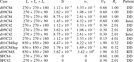
The physical parameters of present simulation cases, in which DD represents double-diffusive convection, RTI means the settling-driven Rayleigh–Taylor instability and ‘Inter.’ means the intermediate pattern.

2.3 Simulation set-up
Following the experiment conducted by Green (Reference Green1987), a volume fraction  $\unicode[STIX]{x1D719}_{0}^{\ast }=8.4\times 10^{-4}$ of particles is set to the upper warm, particle-laden water column as the base case. For major cases, we use four particle sizes,
 $d_{0}=5$,
 $9$,
 $14$ and
 $18~\unicode[STIX]{x03BC}\text{m}$, with the density
 $\unicode[STIX]{x1D70C}_{p}=2.65~\text{kg}~\text{m}^{-3}$. In what follows, we adopt the convention in which each case is named with a combination of two digits of the particle size (in
 $\unicode[STIX]{x03BC}\text{m}$) following the character ‘d’ and the two significant digits after the decimal point of the volume fraction following the character ‘C’, as shown in table 1. The particles are randomly distributed, resulting in a concentration equivalent to the bulk volume fraction in Green (Reference Green1987). The initial temperature profile that results in stable background stratification is given by
 $$\begin{eqnarray}T_{r}^{\ast }(z)=T_{r,low}^{\ast }+0.5(T_{r,up}^{\ast }-T_{r,low}^{\ast })\left[1-\text{erf}\left({\displaystyle \frac{z^{\ast }}{h_{0}}}\right)\right],\end{eqnarray}$$
where  $z$ is the vertical coordinate,
 $h_{0}$ indicates the initial thickness of the interface and
 $T_{r,up}$ and
 $T_{r,low}$ are the reference temperatures at the upper and lower regions, respectively. Following Green (Reference Green1987),
 $T_{r,up}^{\ast }=40.1\,^{\circ }\text{C}$ and
 $T_{r,low}^{\ast }=16.0\,^{\circ }\text{C}$. In (2.23),
 $h_{0}=4.5\times 10^{-4}~\text{m}$ is used to represent the initial sharp gradient between the two layers of uniform temperature in the laboratory setting. In these simulations, although
 $\text{d}T_{r}/\text{d}z$ slowly changes over time due to diffusion, for the sake of convenience, we use its initial value to obtain
 $L$ and calculate
 $\text{d}T_{r}/\text{d}z$ at
 $z=0$. In this study, except for a few cases in which salt is used for background stratification (see § 7),
 $\unicode[STIX]{x1D6FC}=2.07\times 1{0^{-4}\,}^{\circ }\text{C}^{-1}$,
 $\unicode[STIX]{x1D708}=10^{-6}~\text{m}^{2}~\text{s}^{-1}$ and
 $\unicode[STIX]{x1D705}_{T}=1.5\times 10^{-7}~\text{m}^{2}~\text{s}^{-1}$, which gives
 $L=2.22\times 10^{-4}~\text{m}$,
 $U=6.75\times 10^{-4}~\text{m}~\text{s}^{-1}$ and
 $\unicode[STIX]{x1D70F}=3.30\times 10^{-1}~\text{s}$. In thermally stratified cases, with the gravitational force acting in the
 $z$-direction, simulations are conducted in a three-dimensional domain sized
 $L_{x}\times L_{y}\times L_{z}=270\times 270\times 90$ or
 $L_{x}\times L_{y}\times L_{z}=270\times 270\times 180$ with a grid resolution of
 $384\times 384\times 128$ or
 $384\times 384\times 256$, respectively. The domain size with smaller
 $L_{z}$ allows us to focus only on the thermally controlled region (i.e. the region in which the background density gradient is present), whereas the deeper domain (i.e. greater
 $L_{z}$) allows further observation for plumes outside the thermally controlled region. In these simulation cases, the total number of particles ranges from
 $O(10^{6})$ to
 $O(10^{8})$. We adopt the computational time step
 $\unicode[STIX]{x1D6FF}_{t}=10^{-4}~\text{s}$ for all of the cases, such that particles are allowed to move only between two adjacent grid cells at each time step (Chou et al. Reference Chou, Gu and Shao2015). Also, as detailed in appendix A, the small computational time step avoids significant non-physical clustering of particles caused by the numerical instability associated with the explicit Euler scheme for particle tracking. The conditions and set-up for the simulation cases are summarized in table 1. The periodic boundary condition is applied to all horizontal boundaries. Although the random distribution of particles automatically leads to perturbations of infinitesimal wavelengths at the interface, white-noise perturbations with magnitude of
 $O(0.1(T_{r,up}^{\ast }-T_{r,low}^{\ast }))$ are introduced at the sharp temperature gradient, so that instability can be triggered.
3 Sedimentation pattern
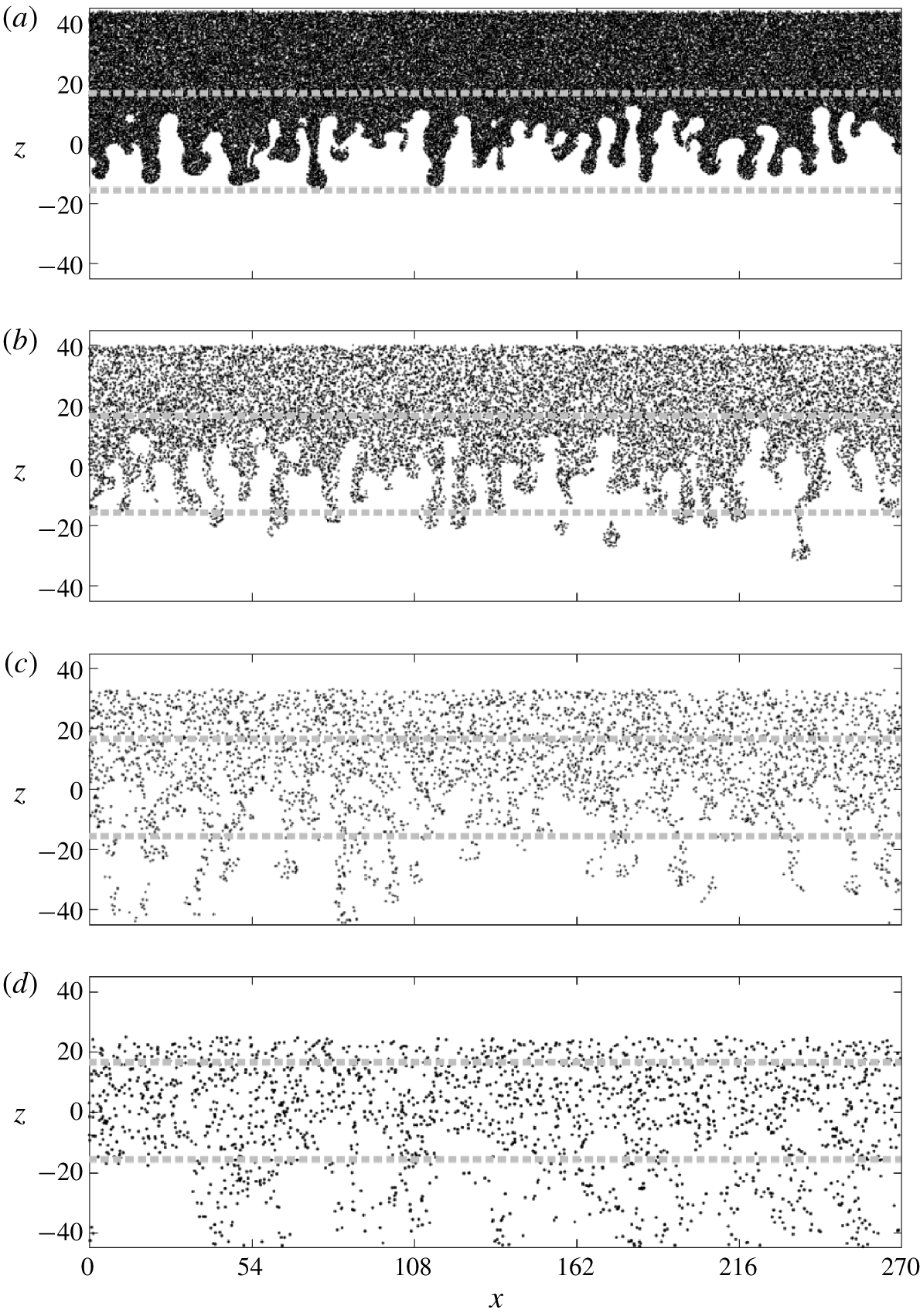
Figure 1 shows representative instantaneous snapshots of suspended particles at the central slice in the  $y$-direction from the four cases of
 $\unicode[STIX]{x1D719}_{0}^{\ast }=8.4\times 10^{-4}$ with various sizes. In cases with small particle sizes (see figure 1a,b), the particle distributions exhibit a finger pattern similar to DD salt fingers except that in this particle case, asymmetry with respect to the central line in the
 $z$-direction (
 $z=0$) can be seen. This is due to gravitational settling of suspended particles, which suppresses the upward motion and elongates the descending plumes. Therefore, as the particle size increases, the asymmetry becomes significant. Another important feature that distinguishes this particle case from the scalar cases (i.e. salt fingers) is the sharp contrast between the particle-laden region and the ambient clear fluid. This is attributed to the zero diffusivity of suspended particles in this study, which resembles the negligible diffusivity
 $({<}O(10^{-14}~\text{m}~\text{s}^{-1}))$ of suspended particles in nature. The infinitesimal diffusivity associated with suspended particles leads to a stronger tendency to form DD plumes than in the salt-finger case due to the greater large-to-small diffusivity ratio. Moreover, the infinitesimal diffusivity associated with suspended particles leads to an apparent pinch-off of the bulbous head of the descending plume from its body when it passes the region of background density gradient, as shown in figure 1(b). As addressed in an early experimental study by Green & Schettle (Reference Green and Schettle1986), this makes the particle-laden plumes that arise from DD sedimentation differ from salt fingers. A detailed discussion of the pinch-off process of the particle-laden plume and its subsequent formation into drops and then a ring torus was given by Chou et al. (Reference Chou, Hung and Chen2020).
Snapshots of the particles at the central slice in the  $y$-direction at
 $t=45.51$ in the cases d05C84 (a), d09C84 (b), d14C84 (c) and d18C84 (d). Grey dashed lines indicate locations where
 $T_{r}=T_{r,low}+0.1(T_{r,up}-T_{r,low})$ (bottom line) and
 $T_{r}=T_{r,low}+0.9(T_{r,up}-T_{r,low})$ (top line). In these panels, point markers are used to represent the positions of the particles located in
 $L_{y}/2-0.1\unicode[STIX]{x1D6FF}y\leqslant y\leqslant L_{y}/2$, in which
 $L_{y}$ is the domain size in the
 $y$-direction and
 $\unicode[STIX]{x1D6FF}y$ is the grid size in the
 $y$-direction.

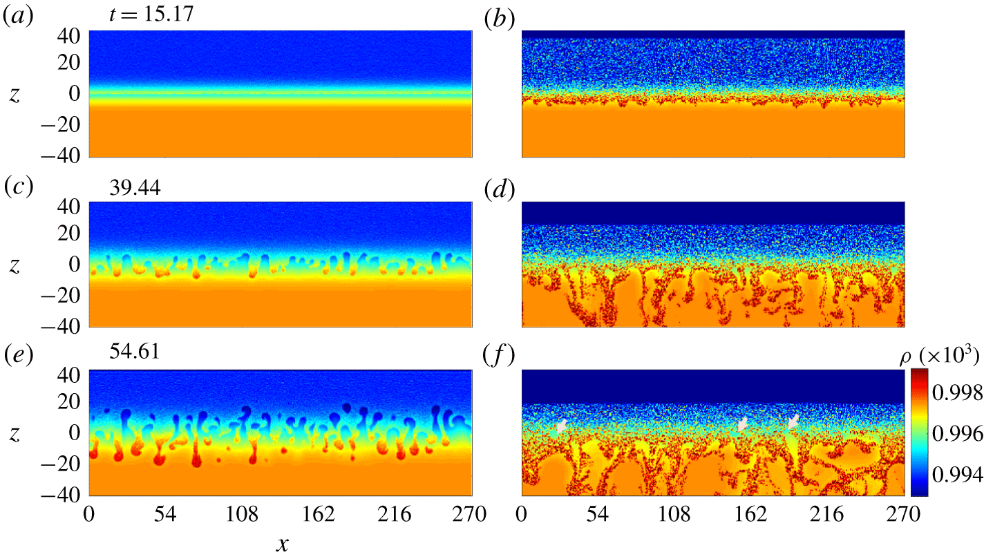
Snapshots of the bulk density at the central slice in the  $y$-direction at representative time steps in cases d05C84 (a,c,e) and d18C84 (b,d,f), showing the time evolution of various patterns of the instability at the particle-laden interface in cases of the small (d05C84) and large (d18C84) particle size. In panel (f), grey arrows are used to point out residual uprising bubbles.

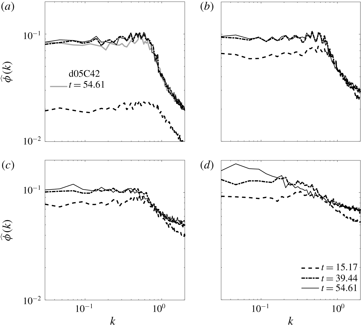
Spectra of the horizontal distribution of the volume fraction  $\unicode[STIX]{x1D719}$ for the cases of d05C84 and d05C42 (a), d09C84 (b), d14C84 (c) and d18C84 (d) at representative time instants. Spectra are sampled at
 $z=-0.35$ in case d05C84 and d05C42,
 $-1.76$ in case d09C84,
 $-4.57$ in case d14C84 and
 $-7.38$ in case d18C84.

Unlike the dominance of double diffusion in cases with small particles, the cases with large particles (figure 1d) show a distinctive pattern in that the horizontal variation seems to be associated with greater wavelengths and the rising plumes are absent. To examine this in more detail, figure 2 compares representative snapshots of the bulk density at the central slice in the  $y$-direction in cases with small (case d05C84) and large (case d18C84) particles. Here, the bulk density is calculated with
 $\unicode[STIX]{x1D70C}=1-\unicode[STIX]{x1D6FC}(T^{\ast }-T_{0}^{\ast })+(r-1)\unicode[STIX]{x1D719}^{\ast }$, in which
 $T_{0}^{\ast }=4\,^{\circ }\text{C}$. As shown in figure 2(a,b), while the growth of the initial perturbations can still hardly be seen in cases with small particles, an unstable, thin layer of excessive density has already developed near the interfacial region due to the fast settling of large particles. Associated with this layer is the sharp reverse density contrast with the lower region, which leads to the onset of RTI and global convection in the lower region of the domain, as shown in figure 2(d,f). In contrast with RTI, which drives global convection, the dominance of thermal exchange in DD sedimentation restricts the instability (i.e. the local density anomaly) within the plume, as shown in figure 1(c,e). As a result, the motion of the downward plume is much slower than that in the settling-driven RTI (i.e. large particle) cases. As shown in figure 2(b), an interesting feature at the early stage in case d18C84 is that the thin layer of excessive density exhibits perturbations of small wavelengths at its lower side. To examine this quantitatively, the spectra of the horizontal distribution of
 $\unicode[STIX]{x1D719}$ sampled near
 $z=0$ in all cases with
 $\unicode[STIX]{x1D719}_{0}^{\ast }=8.4\times 10^{-4}$ corresponding to each time point in figure 2 along with case d05C42 are plotted in figure 3. First, it can be seen that a similar wavenumber,
 $k\approx 0.6$, is found in all cases with smaller particles (i.e. figure 3a–c), which indicates that as long as DD convection occurs, the particle size (i.e. the settling velocity) has no significant effect on the mode of instability. Figure 3(a–c) also shows that, in all cases of double diffusion, the modes change very little over time after the onset of instability. This is a common feature of DD convection, in which the convection (or fingers) is always retained locally. Moreover, as shown in figure 3(a), a comparison with the case of less
 $\unicode[STIX]{x1D719}_{0}^{\ast }$ (d05C42) at
 $t=54.61$ shows that the unstable modes do not differ significantly. Therefore, one can conclude that in the double-diffusion regime, neither the particle size nor the particle concentration can alter the unstable mode.
In the case with a larger particle size, as shown in figure 3(d), the most unstable mode at the early stage in case d18C84 is very close to that in other cases with smaller particles. This corresponds to the small fluctuations at the particle-laden interface, as shown in figure 2(b), which indicates that DD instability still plays a dominant role during the very beginning stage. However, because of the rapid settling in cases with large particles, when the reversed density layer becomes significant such that RTI is dominant, the dominant wavelength increases (i.e. the wavenumber decreases), as shown in figure 3(d). It is worth mentioning that the most unstable mode at  $t=39.44$ in case d18C84 is approximately
 $k=0.2$ (i.e.
 $\unicode[STIX]{x1D706}=2\unicode[STIX]{x03C0}/k=31.43$), which corresponds to the most unstable mode in RTI based on the linear analysis by Chandrasekhar (Reference Chandrasekhar1961). Unlike the double diffusion in which the unstable modes are retained over time during the later time stages (see figure 3), the change in modes in cases with large particles (d18C84) indicates a switch from DD instability to RTI and then global convection (i.e. a greater wavelength in
 $t=54.61$). The distinction between two sedimentation patterns has been examined in previous DNS studies along with the scalar-limit approximation for suspended sediments (Yu et al. Reference Yu, Hsu and Balachandar2014; Burns & Meiburg Reference Burns and Meiburg2015), and a detailed analysis of settling-driven RTI was done in a recent study by Shao et al. (Reference Shao, Hung and Chou2017). In the remainder of this study, we focus our discussion on DD sedimentation and on criteria to distinguish the two sedimentation patterns.
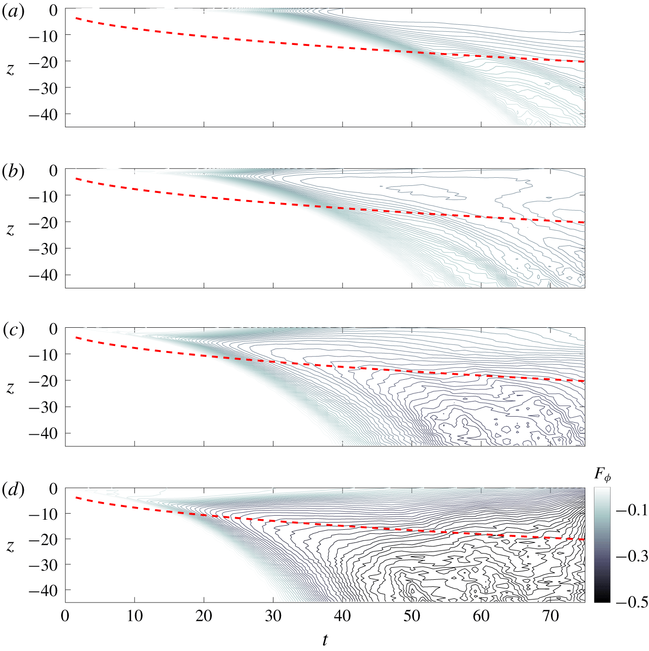
Temporal evolution of normalized horizontal mean particle flux (4.1) (shown by contour lines) in cases d05C84 (a), d09C84 (b), d14C84 (c) and d18C84 (e). Red dashed lines indicate the location where  $T_{r}=T_{r,low}+0.1(T_{r,up}-T_{r,low})$, which are used to indicate the lower bound of the region of the temperature gradient.

4 Mass flux
In this section, the mass fluxes of suspended particles are analysed and compared with existing theories from salt-finger studies. Figure 4 presents the temporal evolution (by contour lines) of the vertical distribution of the horizontal mean particle fluxes normalized with  $\unicode[STIX]{x1D719}_{0}$ (
 $\unicode[STIX]{x1D719}_{0}=1$) in the lower half of the domain for all cases of
 $\unicode[STIX]{x1D719}_{0}^{\ast }=8.4\times 10^{-4}$. Here, for the sake of convenience, without tracking particles, the approximation for the particle flux
 $F_{\unicode[STIX]{x1D719}}$ is obtained with
 $$\begin{eqnarray}F_{\unicode[STIX]{x1D719}}={\displaystyle \frac{1}{A}}\iint _{A}\unicode[STIX]{x1D719}\boldsymbol{u}_{c}\boldsymbol{\cdot }\hat{\boldsymbol{e}}_{3}\,\text{d}x\,\text{d}y,\end{eqnarray}$$
where  $A$ is the cross-sectional area in the vertical direction of the domain. In figure 4, all cases show that the flux attains its greatest magnitude near the particle-laden interface, which is initially located at
 $z=0$ and descends slightly due to
 $\boldsymbol{w}_{s}$. The flux decreases with the downward distance from the interface. Moreover, in all cases except d18C84, the flatter contours within the region of the background temperature gradient (above the red dashed lines) in the latter stage (i.e.
 $t>30$) imply that the temporal variations are relatively slow within the region compared to those outside the region (i.e. below the red dashed lines), particularly in cases d05C84 and d09C84 (see figure 4a,b). This somewhat indicates the slow evolution of the flux when it is dominated by the thermal effect and the accelerated evolution in the absence of the thermal effect outside the region of the temperature gradient. In case d18C84, as shown in figure 4(d), very little difference can be found between the regions inside and outside the temperature gradient, particularly when
 $t>60$, which implies the lack of significance of the thermal effect in cases with large particles. Due to the fairly slow temporal evolution, we treat the later time stage
 $t>30$ as the quasi-steady state, and in the following analysis, we first focus on the flux sampled within the region of the temperature gradient (i.e. above the red dashed lines in figure 4), which hereafter is called the thermally controlled region. For the regions outside the thermally controlled region in which the temperature gradient vanishes, convective motion is closely related to secondary instability; a detailed discussion is given in § 8. It is worth mentioning that, as shown in figure 4(a–c), in the three cases of double-diffusive convection, the hydrodynamically induced fluxes do not differ significantly from one another due to the equal buoyant forcing. However, as shown in figure 4(d), the flux can be greatly enhanced when the sedimentation is dominated by settling-driven RTI.
4.1 Flux ratio
It is important to examine the analogy between our simulation results and the existing theories in the context of DD salt fingers. We adopt the theoretical arguments from Stern (Reference Stern1976), who derived the analytical expression for the total buoyant flux,  $F_{tot}$, for salt fingers. Before discussing its analogy with those of our particle cases, a brief review of the theoretical results in Stern (Reference Stern1976) is given as follows.
Under the condition of quasi-steady state, Stern (Reference Stern1976) showed that
 $$\begin{eqnarray}{\displaystyle \frac{F_{tot,S}^{3/2}}{(\unicode[STIX]{x1D6FD}\unicode[STIX]{x0394}S_{r}^{\ast })^{2}(g\unicode[STIX]{x1D705}_{T})^{1/2}}}\propto R_{c,S}^{1/2}(1-R_{f,S})^{3/2}\left(R_{f,S}-{\displaystyle \frac{\unicode[STIX]{x1D705}_{S}}{\unicode[STIX]{x1D705}_{T}}}\right)^{1/2},\end{eqnarray}$$
where the subscript  $S$ represents the salinity field,
 $\unicode[STIX]{x0394}S_{r}$ is the initial (maximum) salinity difference between the two layers,
 $\unicode[STIX]{x1D6FD}$ is the density expansion coefficient of salt,
 $\unicode[STIX]{x1D705}_{S}$ is the diffusivity for salt,
 $$\begin{eqnarray}R_{c,S}={\displaystyle \frac{F_{tot,S}}{\displaystyle \unicode[STIX]{x1D708}\left(\unicode[STIX]{x1D6FC}{\displaystyle \frac{\text{d}T_{r}^{\ast }}{\text{d}z^{\ast }}}-\unicode[STIX]{x1D6FD}{\displaystyle \frac{\text{d}S_{r}^{\ast }}{\text{d}z^{\ast }}}\right)}}\end{eqnarray}$$
is the ratio between the total buoyant flux and the conductive flux, in which  $S_{r}$ is the background (base-state) salinity, and
 $$\begin{eqnarray}R_{f,S}={\displaystyle \frac{\unicode[STIX]{x1D6FC}\overline{w_{c}^{\ast \prime }T^{\ast \prime }}}{\unicode[STIX]{x1D6FD}\overline{w_{c}^{\ast \prime }S^{\ast \prime }}}}\end{eqnarray}$$
is the buoyant flux ratio between the temperature and salt, in which the prime indicates a deviation from the basic state (i.e.  $\boldsymbol{u}_{c}=0$ and
 $\unicode[STIX]{x1D719}=0$ at
 $z<0$), and the overbar denotes the planar average in the horizontal direction. It is straightforward to show that if
 $R_{f,S}$ is a constant, scaling for
 $F_{tot,S}$ can be obtained as
 $$\begin{eqnarray}F_{tot,S}\propto \left({\displaystyle \frac{g\unicode[STIX]{x1D705}_{T}}{\unicode[STIX]{x1D708}}}\right)^{1/2}(\unicode[STIX]{x1D6FD}\unicode[STIX]{x0394}S_{r}^{\ast })^{2}\left(\unicode[STIX]{x1D6FC}{\displaystyle \frac{\text{d}T_{r}^{\ast }}{\text{d}z^{\ast }}}-\unicode[STIX]{x1D6FD}{\displaystyle \frac{\text{d}S_{r}^{\ast }}{\text{d}z^{\ast }}}\right)^{-1/2}.\end{eqnarray}$$
Indeed, a feature such that  $R_{f}$ becomes constant, particularly for large (lower-to-upper) density ratio (i.e.
 $(\unicode[STIX]{x1D6FC}\unicode[STIX]{x0394}T_{r}^{\ast })/(\unicode[STIX]{x1D6FD}\unicode[STIX]{x0394}S_{r}^{\ast })>2$), has been confirmed in experimental (Turner Reference Turner1967; Schmitt Reference Schmitt1979a; Taylor & Bucens Reference Taylor and Bucens1989), numerical (Shen Reference Shen1993, Reference Shen1995) and theoretical (Kunze Reference Kunze1987; Stern Reference Stern1976) studies of salt fingers. In experimental studies,
 $R_{f,S}$ values range mostly from 0.4 to 0.6. Stern (Reference Stern1976) argued that
 $R_{f,S}=(3\unicode[STIX]{x1D705}_{S}/\unicode[STIX]{x1D705}_{T}+1)/4$ maximizes the total buoyant flux. For our case of suspended particles with zero diffusivity, this gives
 $R_{f}=0.25$.
For the present temperature–particle system, one may simply replace  $S^{\ast }$ in (4.2), (4.3) and (4.4) with
 $\unicode[STIX]{x1D719}^{\ast }$, and define the buoyant flux ratio for the temperature–particle system as
 $$\begin{eqnarray}R_{f}={\displaystyle \frac{\unicode[STIX]{x1D6FC}\overline{w_{c}^{\ast \prime }T^{\ast \prime }}}{(r-1)\overline{w_{c}^{\ast \prime }\unicode[STIX]{x1D719}^{\ast \prime }}}}.\end{eqnarray}$$
It should also be noted that, as the initial state  $\unicode[STIX]{x1D719}^{\ast }$ is given by a concentration jump (i.e.
 $\unicode[STIX]{x1D719}^{\ast }=\unicode[STIX]{x1D719}_{0}^{\ast }$ or
 $0$), without diffusivity,
 $\text{d}\unicode[STIX]{x1D719}_{0}^{\ast }/\text{d}z$ vanishes in the regions below and above the interface of the concentration jump. In other words, with zero diffusivity, the conductive flux of
 $\unicode[STIX]{x1D719}^{\ast }$ is zero. As a result,
 $R_{c}$ for this temperature–particle system can be written as
 $$\begin{eqnarray}R_{c}={\displaystyle \frac{F_{tot}}{\displaystyle \unicode[STIX]{x1D708}\unicode[STIX]{x1D6FC}{\displaystyle \frac{\text{d}T_{r}^{\ast }}{\text{d}z^{\ast }}}}}.\end{eqnarray}$$
The final scaling of  $\overline{w_{c}^{\ast \prime }\unicode[STIX]{x1D719}^{\ast \prime }}$ can thus be obtained from (4.2) by replacing
 $S$ with
 $\unicode[STIX]{x1D6F7}$,
 $R_{c,S}$ with the
 $R_{c}$ of (4.7) and
 $\unicode[STIX]{x1D6FD}$ with
 $(r-1)$. If
 $R_{f}$ becomes constant, under the limit of
 $\unicode[STIX]{x1D705}_{\unicode[STIX]{x1D719}}=0$, this gives
 $$\begin{eqnarray}\overline{w_{c}^{\ast \prime }\unicode[STIX]{x1D719}^{\ast \prime }}\propto (r-1)\left({\displaystyle \frac{g\unicode[STIX]{x1D705}_{T}}{\unicode[STIX]{x1D708}}}\right)^{1/2}\unicode[STIX]{x0394}\unicode[STIX]{x1D719}_{0}^{\ast 2}\left(\unicode[STIX]{x1D6FC}{\displaystyle \frac{\text{d}T_{r}^{\ast }}{\text{d}z^{\ast }}}\right)^{-1/2},\end{eqnarray}$$
where we have applied the relationship  $F_{tot}=(r-1)\overline{w_{c}^{\ast \prime }\unicode[STIX]{x1D719}^{\ast \prime }}(1+R_{f})$.
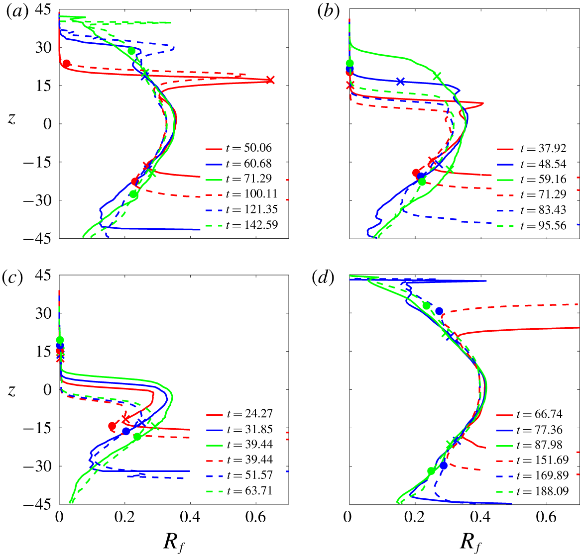
Figure 5 presents the profiles of  $R_{f}$ at representative time points with various particle sizes and two initial concentrations, along with the salt-finger case for comparison. It can be seen that within the thermally controlled region, except the abrupt drop at the upper region caused by the suppression of the upward flux due to particle settling,
 $R_{f}$ values range from 0.20 to 0.33 in particle cases (figure 5a–c). This does not differ significantly among cases with different particle sizes, which indicates that, in this study, as long as the sedimentation pattern is in the DD regime (i.e. small particles), particle size has a negligible effect on the buoyant flux ratio
 $R_{f}$. In figure 5, the highest
 $R_{f}$ at the central region is due to the maximum gradient of the reference temperature (
 $\text{d}T_{r}/\text{d}z$), and it decreases with the distance from the vertical centre because of the diffusion of
 $T_{r}$ (i.e. low
 $\text{d}T_{r}/\text{d}z$). For the lower concentration, it can be found that distributions of
 $R_{f}$ are similar to those in the higher
 $\unicode[STIX]{x1D719}_{0}^{\ast }$ but slightly smaller in magnitude. The trend of constant
 $R_{f}$ with
 $\unicode[STIX]{x1D719}_{0}^{\ast }$ in the present study is consistent to previous studies of salt fingers, but here, the values ranging from 0.20 to 0.33 are generally lower than those found in previous studies. For comparison, figure 5(d) presents profiles of
 $R_{f,S}$ values at representative time steps in the salt-finger cases with the same buoyant and thermal conditions as in figure 5(a–c). Again, the slowly varying vertical distributions of
 $R_{f}$ in the thermally controlled region are similar to those found in the particle cases. However, the magnitude of
 $R_{f}$ is typically greater in the salt-finger case than in the particle-laden case and, because there is no gravitational settling, the distributions are more symmetric about
 $z=0$. The greater
 $R_{f}$ for salt fingers is attributed to the greater diffusivity of salt, which, compared to the particle-laden fingers, significantly reduces the contrast in the concentration between adjacent fingers (i.e. reducing
 $S^{\prime }$).
If one treats  $R_{f}$ as a constant, under the same thermal condition (i.e. the same temperature gradient), equation (4.8) simply gives the relationship
 $$\begin{eqnarray}\overline{w_{c}^{\ast \prime }\unicode[STIX]{x1D719}^{\ast \prime }}\propto \unicode[STIX]{x1D719}_{0}^{\ast 2},\end{eqnarray}$$
or its non-dimensional form obtained by normalizing  $\unicode[STIX]{x1D719}^{\ast }$ with
 $\unicode[STIX]{x1D719}_{0}^{\ast }$ and
 $w$ with
 $U$, i.e.
 $$\begin{eqnarray}\overline{w_{c}^{\prime }\unicode[STIX]{x1D719}^{\prime }}\propto \unicode[STIX]{x1D719}_{0}^{\ast }.\end{eqnarray}$$
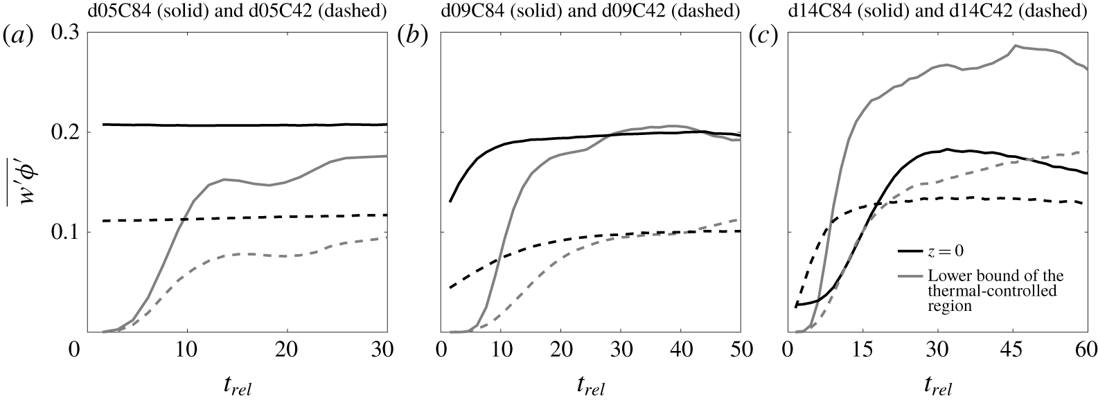
Figure 6 shows the time histories of the (dimensionless) fluctuation flux  $\overline{w_{c}^{\prime }\unicode[STIX]{x1D719}^{\prime }}$ at both the centre (
 $z=0$) and the lower bound of the thermally controlled region in cases corresponding to figure 5(a–c). Figure 6(a,b) shows that the buoyant flux
 $\overline{w^{\prime }\unicode[STIX]{x1D719}^{\prime }}$ in the case with the higher
 $\unicode[STIX]{x1D719}_{0}^{\ast }$ is almost twice that in the case with lower
 $\unicode[STIX]{x1D719}_{0}^{\ast }$, which confirms the identity given by (4.10) in cases with small particles. For cases with larger particles (e.g. cases d14C84 and d14C42), the sedimentation pattern may not be the DD type for the case of smaller
 $\unicode[STIX]{x1D719}_{0}^{\ast }$ (d14C42) (see § 7), and (4.10) may not be valid, as shown in figure 6(c).
Vertical profiles of  $R_{f}$ at representative time points in the case combinations of d05C84 and d05C42 (a), d09C84 and d09C42 (b), d14C84 and d14C42 (c) and SFC84 and SFC42 (d). In each panel, crosses mark the lower and upper bounds of the thermally controlled region for cases with a higher initial concentration (
 $\unicode[STIX]{x1D719}_{0}^{\ast }=8.4\times 10^{-4}$ (in volume concentration)), and solid circles mark those for lower initial concentrations (
 $\unicode[STIX]{x1D719}_{0}^{\ast }=4.2\times 10^{-4}$ (in volume concentration)).

Time histories of the (dimensionless) fluctuation flux  $\overline{w_{c}^{\prime }\unicode[STIX]{x1D719}^{\prime }}$ at both the centre (
 $z=0$) and the lower bound of the thermally controlled region in cases corresponding to figure 5(a–c). Here, the time history is taken relative to the time point at which the descending plumes begin to pass through the lower bound of the thermally controlled region.

5 Energy budget
This section includes the energy budget analysis. The object of this analysis is to quantify the enhancement of sedimentation flux due to the resulting convective motion and to derive the scale for the velocity as a bulk parameter. Here, for the sake of simplicity, we focus only on cases with  $\unicode[STIX]{x1D719}_{0}^{\ast }=8.4\times 10^{-4}$, but the findings will also be applied to cases with a lower
 $\unicode[STIX]{x1D719}_{0}^{\ast }$.
Following Chou & Shao (Reference Chou and Shao2016), if both phases are static in the initial state, the energy budget of the present Eulerian–Lagrangian system for a horizontally periodic domain at time  $t=\widetilde{t}$ is obtained from a combination of the inner product of
 $\boldsymbol{u}_{c}$ to the momentum equations of the continuum phase (2.16) and the inner product of
 $\boldsymbol{u}_{p,k}$ to the momentum equation of the particle phase. As detailed in Chou & Shao (Reference Chou and Shao2016), the resulting dimensionless equation for energy budget can be written as
 $$\begin{eqnarray}KE(\tilde{t})=\unicode[STIX]{x0394}PE_{p}(\tilde{t})+\unicode[STIX]{x0394}PE_{T}(\tilde{t})-\unicode[STIX]{x1D6E9}(\tilde{t})-DR(\tilde{t}).\end{eqnarray}$$
In (5.1),
 $$\begin{eqnarray}KE(\tilde{t})=r\unicode[STIX]{x1D719}_{0}^{\ast }\unicode[STIX]{x1D719}_{p}\mathop{\sum }_{k=1}^{N_{tot}}{\displaystyle \frac{1}{2}}|\boldsymbol{u}_{p,k}|^{2}+\int _{\unicode[STIX]{x1D6FA}}{\displaystyle \frac{1}{2}}|\boldsymbol{u}_{c}|^{2}\,\text{d}V\end{eqnarray}$$
is the total kinetic energy, where  $N_{tot}$ is the number of particles, and
 $\int _{\unicode[STIX]{x1D6FA}}(\cdot )\,\text{d}V$ represents integration over the entire computational domain,
 $$\begin{eqnarray}\unicode[STIX]{x0394}PE_{p}(\tilde{t})=-\int _{t=0}^{\tilde{t}}\frac{Pr}{R_{\unicode[STIX]{x1D70C}}}\unicode[STIX]{x1D719}_{p}\mathop{\sum }_{k=1}^{N_{tot}}\boldsymbol{u}_{p,k}\boldsymbol{\cdot }\hat{\boldsymbol{e}}_{3}\,\text{d}t\end{eqnarray}$$
is the potential energy released by the settling of particles,
 $$\begin{eqnarray}\unicode[STIX]{x0394}PE_{T}(\tilde{t})=\int _{t=0}^{\tilde{t}}\int _{\unicode[STIX]{x1D6FA}}Pr\unicode[STIX]{x0394}T\boldsymbol{u}_{c}\boldsymbol{\cdot }\hat{\boldsymbol{e}}_{3}\,\text{d}V\,\text{d}t,\end{eqnarray}$$
is the potential energy released due to the change in temperature,
 $$\begin{eqnarray}DR(\tilde{t})=\int _{t=0}^{\tilde{t}}{\displaystyle \frac{r\unicode[STIX]{x1D719}_{0}^{\ast }}{St}}\unicode[STIX]{x1D719}_{p}\mathop{\sum }_{k=1}^{N_{tot}}|\boldsymbol{u}_{p,k}-\boldsymbol{u}_{c\mid p,k}|^{2}\,\text{d}t\end{eqnarray}$$
is the drag dissipation due to particle–fluid interaction and
 $$\begin{eqnarray}\unicode[STIX]{x1D6E9}(\tilde{t})=-\int _{t=0}^{\tilde{t}}\int _{\unicode[STIX]{x1D6FA}}Pr\boldsymbol{u}_{c}\boldsymbol{\cdot }(\unicode[STIX]{x1D735}\boldsymbol{\cdot }\unicode[STIX]{x1D64F})\,\text{d}V\,\text{d}t\end{eqnarray}$$
is the shear dissipation, where  $\unicode[STIX]{x1D64F}=\unicode[STIX]{x1D735}\boldsymbol{u}_{c}$ is the dimensionless stress tensor. In what follows, each term in (5.1) is normalized using the initial potential energy of the particle phase,
 $$\begin{eqnarray}PE_{p,0}=\frac{Pr}{R_{\unicode[STIX]{x1D70C}}}\unicode[STIX]{x1D719}_{p}\mathop{\sum }_{k=1}^{N_{tot}}\unicode[STIX]{x0394}H_{0,k},\end{eqnarray}$$
where  $\unicode[STIX]{x0394}H_{0,k}$ is the (dimensionless) distance between the initial position of the
 $k$th particle and the bottom of the domain.
Here, we are interested in the hydrodynamics-induced sedimentation enhancement,  $SE$, apart from the gravitational settling of individual particles. Because settling of individual particles is due to drag, the drag dissipation term,
 $DR$ (5.5), accounts for its contribution to
 $\unicode[STIX]{x0394}PE_{p}$. One can thus have
 $$\begin{eqnarray}\unicode[STIX]{x0394}PE_{p}(\tilde{t})=SE(\tilde{t})+DR(\tilde{t}),\end{eqnarray}$$
which indicates that  $SE$ arises from all the other contributions to
 $\unicode[STIX]{x0394}PE_{p}$ in addition to
 $DR$. In cases with various particle sizes, larger particles settle faster than small particles and can leave the computational domain quickly. Once particles leave the domain, the analysis is no longer valid. Also, as demonstrated below, due to the lower number density of particles (i.e. less homogeneous) and faster gravitational settling with the same volume concentration, larger particles are typically associated with more pronounced perturbations at the particle-laden interface. This results in a shorter period for the initial development of flow instabilities and leads to the subsequent convective motion sooner than that due to smaller particles. Therefore, it may not be relevant to analyse the energy budget between different particle sizes on the same time basis. Instead, to show more clearly the contributions of each term to sedimentation, we perform the analysis based on the same final
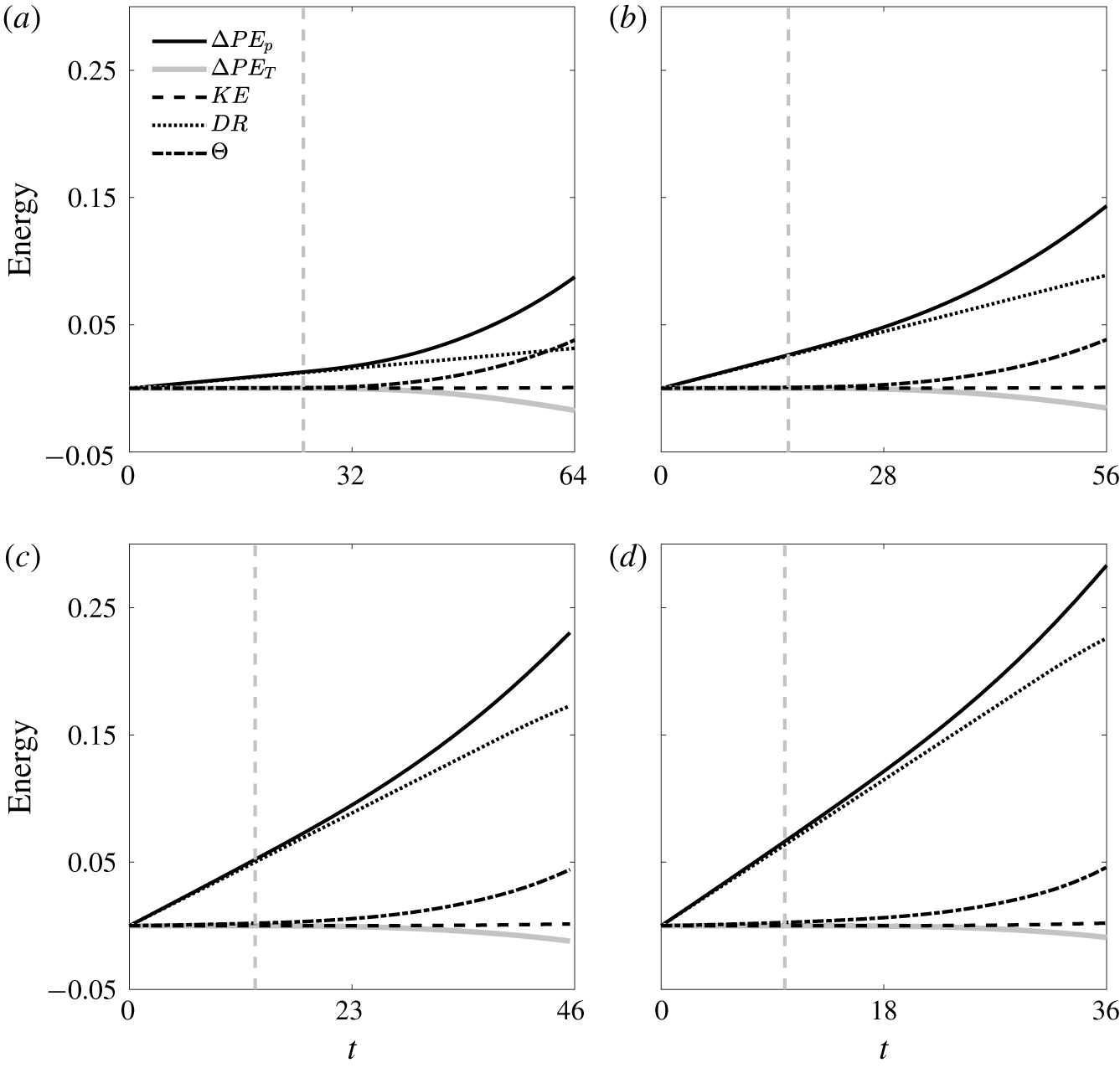
 $SE$, which gives the time zones of our following analysis for each case. Figure 7 shows the time histories of each term in (5.1) in all cases of
 $\unicode[STIX]{x1D719}_{0}^{\ast }=8.4\times 10^{-4}$. It can be seen that the evolution of the energy budget can be divided into two regimes, as separated by the grey dashed lines in figure 7. The first (i.e. the left side of the grey dashed line) corresponds to a stage in which
 $\unicode[STIX]{x0394}PE_{p}\approx DR$. At this stage, flow instabilities are insignificant and particle settling is caused mainly by the gravitational settling of individual particles. The second stage corresponds to the later time stage in which
 $\unicode[STIX]{x0394}PE_{p}$ deviates from
 $DR$, as shown on the right side of the grey line in each panel of figure 7, which is a result of flow instabilities and the subsequent convective motion. Figure 7 shows that cases with larger particles are associated with a shorter initial time stage. As shown in figure 7,
 $KE$ is negligible compared with the other quantities in all cases. Therefore, according to (5.1) and (5.8),
 $SE$ can be written as
 $$\begin{eqnarray}SE(\tilde{t})\approx \unicode[STIX]{x1D6E9}(\tilde{t})-\unicode[STIX]{x0394}PE_{T}(\tilde{t}),\end{eqnarray}$$
indicating that the sedimentation enhancement is dominated by a combined result of hydrodynamics and the thermal effect, in which the former is dominated by shear stresses, resulting in viscous dissipation in the energy budget.
Time evolution of energy budgets (5.1) for cases d05C84 (a), d09C84 (b), d14C84 (c) and d18C84 (d).

Time evolution of the relative contribution of  $-\unicode[STIX]{x0394}PE_{T}$ to the sedimentation enhancement (
 $SE$) in all cases with
 $\unicode[STIX]{x1D719}_{0}^{\ast }=8.4\times 10^{-4}$ and the salt-finger case. In the salt-finger case, because
 $DR=0$,
 $SE$ is replaced with
 $\unicode[STIX]{x0394}PE_{p}$.

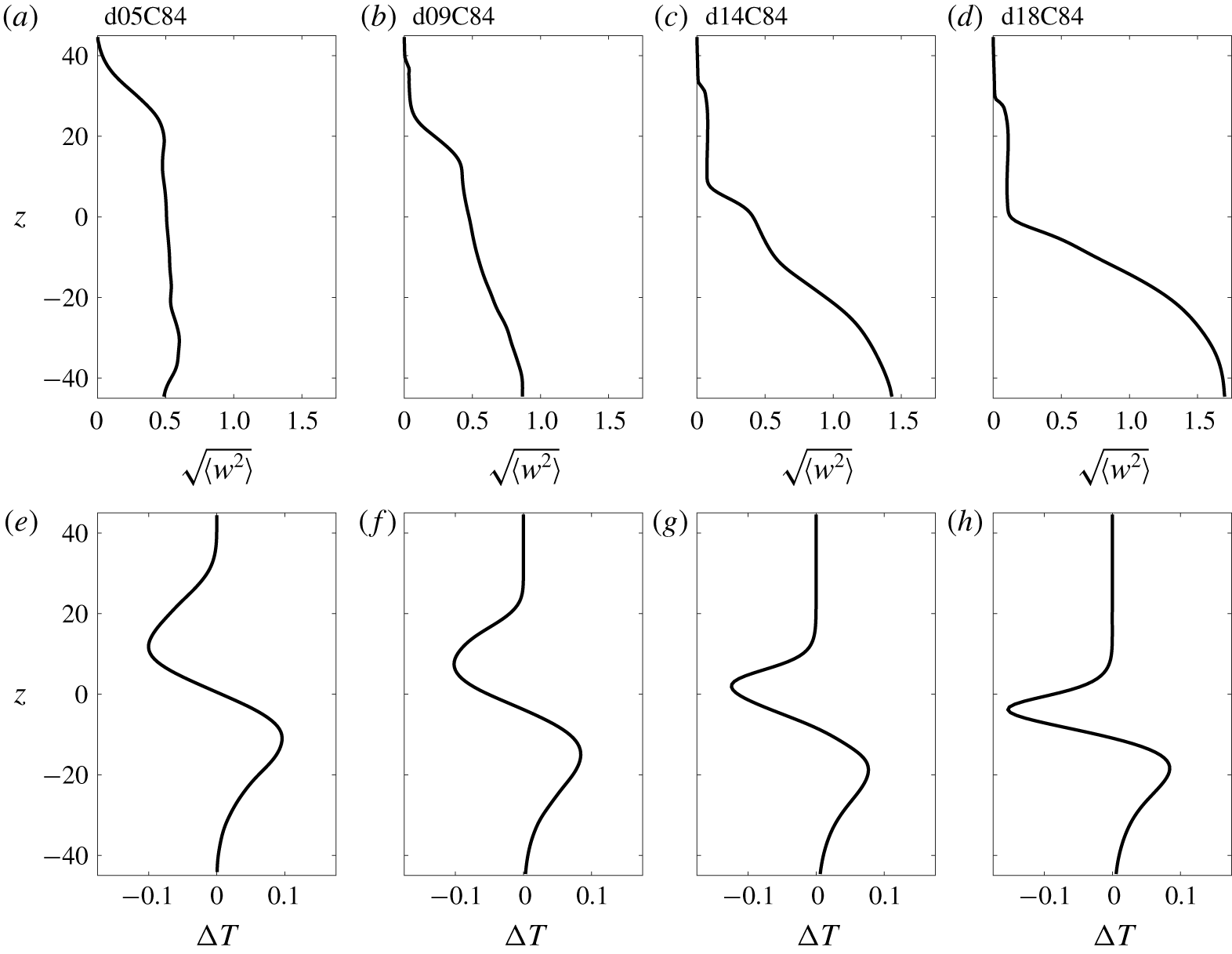
Vertical profiles of the horizontal root mean squared vertical velocity,  $\sqrt{\langle w^{2}\rangle }$, (a–d) and the corresponding horizontally averaged temperature anomaly,
 $\langle \unicode[STIX]{x0394}T\rangle$, (e–h) at the end of the energy budget analysis in each simulation run (i.e.
 $t=64$ in case d05C84, 56 in d09C84, 46 in d14C84 and 36 in d18C84).

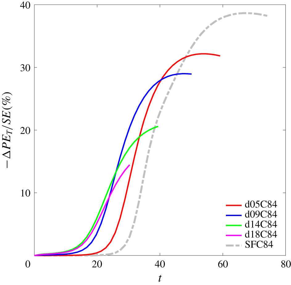
To demonstrate the thermal contribution to settling enhancement for these cases, figure 8 presents the proportion of  $-\unicode[STIX]{x0394}PE_{T}$ to
 $SE$ in all cases of
 $\unicode[STIX]{x1D719}_{0}^{\ast }=8.4\times 10^{-4}$ along with the salt-finger case, for which
 $\unicode[STIX]{x0394}PE_{p}$ is replaced with
 $SE$ because
 $DR=0$. It can be seen that, typically, the relative contribution of
 $-\unicode[STIX]{x0394}PE_{T}$ to
 $SE$ is insignificant at the beginning stage due to slow motion of particle-laden plumes. It increases rapidly when convective motion is dominant and reaches a peak value. Figure 8 clearly shows that the final contribution of temperature increases as the particle size decreases and attains its maximum in the salt-finger case (
 $w_{s}=0$). This is because the gravitational settling of individual particles suppresses the motion of the rising plumes, such that the vertical velocity on the upper side of the particle-laden interface (i.e. the rising motion) is weaker than that of the descending plumes on the lower side of the interface. As expressed by (5.4) and (5.9), the weak vertical velocity thus leads to a lesser contribution of
 $\unicode[STIX]{x0394}PE_{T}$. To demonstrate this, figure 9 presents the vertical profiles of the horizontally root-mean-squared vertical velocity (
 $\sqrt{\langle w^{2}\rangle }$) (a–d) and the horizontally averaged temperature anomaly (
 $\overline{\unicode[STIX]{x0394}T}$) (e–h) at the final time step corresponding to each case in figure 7. It shows that when the particles are small, the distribution is relatively symmetrical for
 $\sqrt{\langle w^{2}\rangle }$ (see figure 9a) and antisymmetrical for
 $\langle \unicode[STIX]{x0394}T\rangle$ (figure 9e) about
 $z=0$. Moreover, figure 9(b–d) shows the increasing suppression of the vertical momentum in the upper half of the domain as the particle size increases. As a result, as shown in figure 9(f–h), the negative temperature anomaly in the upper region becomes confined more to the vertical centre of the domain as the particle size increases, whereas the positive anomaly in the lower region does not differ significantly between the cases. The suppression of the plume’s upward motion leads to a lower thermal contribution to particle settling in cases with larger particles.
6 Velocity scaling
In this section, velocity scaling is obtained from the energy budget analysis. The scaling can be further used to distinguish RTI-dominant and DD sedimentation for a given particle size, concentration and thermal conditions. We begin from the temporal evolution of the energy budget. Because  $KE$ was found to be negligible, the shear dissipation is in balance with the release of the total potential energy and drag dissipation, i.e.
 $$\begin{eqnarray}{\displaystyle \frac{\text{d}}{\text{d}t}}(\unicode[STIX]{x0394}PE_{p}+\unicode[STIX]{x0394}PE_{T}-DR)={\displaystyle \frac{\text{d}}{\text{d}t}}\unicode[STIX]{x1D6E9}.\end{eqnarray}$$
Substitution of (2.13) into (5.3) for each  $k$th particle and taking of the time derivative gives
 $$\begin{eqnarray}{\displaystyle \frac{\text{d}}{\text{d}t}}\unicode[STIX]{x0394}PE_{p}=-{\displaystyle \frac{Pr}{R_{\unicode[STIX]{x1D70C}}}}\unicode[STIX]{x1D719}_{p}\mathop{\sum }_{k=1}^{N_{tot}}\left(\boldsymbol{u}_{c\mid p,k}+\boldsymbol{w}_{s}-St{\displaystyle \frac{\text{d}\boldsymbol{u}_{p,k}}{\text{d}t}}\right)\boldsymbol{\cdot }\hat{\boldsymbol{e}}_{3}.\end{eqnarray}$$
Likewise, for the temporal evolution of the drag dissipation, we obtain
 $$\begin{eqnarray}{\displaystyle \frac{\text{d}}{\text{d}t}}DR={\displaystyle \frac{r\unicode[STIX]{x1D719}_{0}^{\ast }}{St}}\unicode[STIX]{x1D719}_{p}\mathop{\sum }_{k=1}^{N_{tot}}\left(|\boldsymbol{w}_{s}|^{2}-2St\boldsymbol{w}_{s}\boldsymbol{\cdot }{\displaystyle \frac{\text{d}\boldsymbol{u}_{p,k}}{\text{d}t}}+St^{2}\left|{\displaystyle \frac{\text{d}\boldsymbol{u}_{p,k}}{\text{d}t}}\right|^{2}\right).\end{eqnarray}$$
Also, given the present dimensional parameters (see (2.12)), we can rewrite the dimensionless settling velocity (2.14) as
 $$\begin{eqnarray}\boldsymbol{w}_{s}=-{\displaystyle \frac{Pr}{R_{\unicode[STIX]{x1D70C}}}}{\displaystyle \frac{St}{r\unicode[STIX]{x1D719}_{0}^{\ast }}}\hat{\boldsymbol{e}}_{3}.\end{eqnarray}$$
Now, using the relationship given by (6.4), equation (6.3) can be rewritten as
 $$\begin{eqnarray}{\displaystyle \frac{\text{d}}{\text{d}t}}DR=-{\displaystyle \frac{Pr}{R_{\unicode[STIX]{x1D70C}}}}\unicode[STIX]{x1D719}_{p}\mathop{\sum }_{k=1}^{N_{tot}}\boldsymbol{w}_{s}\boldsymbol{\cdot }\hat{\boldsymbol{e}}_{3}+2{\displaystyle \frac{Pr}{R_{\unicode[STIX]{x1D70C}}}}\unicode[STIX]{x1D719}_{p}St\mathop{\sum }_{k=1}^{N_{tot}}{\displaystyle \frac{\text{d}\boldsymbol{u}_{p,k}}{\text{d}t}}\boldsymbol{\cdot }\hat{\boldsymbol{e}}_{3}+r\unicode[STIX]{x1D719}_{0}^{\ast }\unicode[STIX]{x1D719}_{p}St\mathop{\sum }_{k=1}^{N_{tot}}\left|{\displaystyle \frac{\text{d}\boldsymbol{u}_{p,k}}{\text{d}t}}\right|^{2}.\end{eqnarray}$$
Moreover, subtracting (6.5) from (6.2) gives
 $$\begin{eqnarray}\displaystyle {\displaystyle \frac{\text{d}}{\text{d}t}}(\unicode[STIX]{x0394}PE_{p}-DR) & = & \displaystyle -{\displaystyle \frac{Pr}{R_{\unicode[STIX]{x1D70C}}}}\unicode[STIX]{x1D719}_{p}\mathop{\sum }_{k=1}^{N_{tot}}\boldsymbol{u}_{c\mid p,k}\boldsymbol{\cdot }\hat{\boldsymbol{e}}_{3}\nonumber\\ \displaystyle & & \displaystyle -\,{\displaystyle \frac{Pr}{R_{\unicode[STIX]{x1D70C}}}}\unicode[STIX]{x1D719}_{p}St\mathop{\sum }_{k=1}^{N_{tot}}{\displaystyle \frac{\text{d}\boldsymbol{u}_{p,k}}{\text{d}t}}\boldsymbol{\cdot }\hat{\boldsymbol{e}}_{3}-r\unicode[STIX]{x1D719}_{0}^{\ast }\unicode[STIX]{x1D719}_{p}St\mathop{\sum }_{k=1}^{N_{tot}}\left|{\displaystyle \frac{\text{d}\boldsymbol{u}_{p,k}}{\text{d}t}}\right|^{2}.\end{eqnarray}$$
In the present cases with small particles for which  $St\ll 1$, equation (6.6) gives
 $$\begin{eqnarray}{\displaystyle \frac{\text{d}}{\text{d}t}}(\unicode[STIX]{x0394}PE_{p}-DR)\approx -{\displaystyle \frac{Pr}{R_{\unicode[STIX]{x1D70C}}}}\unicode[STIX]{x1D719}_{p}\mathop{\sum }_{k=1}^{N_{tot}}\boldsymbol{u}_{c\mid p,k}\boldsymbol{\cdot }\hat{\boldsymbol{e}}_{3},\end{eqnarray}$$
which indicates that with a small  $St$, the settling enhancement is mainly due to the bulk buoyancy effect of the suspended particles. Moreover, using (5.4) and (6.7), one can obtain the left-hand side of (6.1) as
 $$\begin{eqnarray}\displaystyle {\displaystyle \frac{\text{d}}{\text{d}t}}(\unicode[STIX]{x0394}PE_{p}+\unicode[STIX]{x0394}PE_{T}-DR) & {\approx} & \displaystyle -{\displaystyle \frac{Pr}{R_{\unicode[STIX]{x1D70C}}}}\unicode[STIX]{x1D719}_{p}\mathop{\sum }_{k=1}^{N_{tot}}\boldsymbol{u}_{c\mid p,k}\boldsymbol{\cdot }\hat{\boldsymbol{e}}_{3}+\int _{\unicode[STIX]{x1D6FA}}Pr\unicode[STIX]{x0394}T\boldsymbol{u}_{c}\boldsymbol{\cdot }\hat{\boldsymbol{e}}_{3}\,\text{d}V\nonumber\\ \displaystyle & = & \displaystyle -{\displaystyle \frac{Pr}{R_{\unicode[STIX]{x1D70C}}}}(1-R_{\unicode[STIX]{x1D70C}}R_{B})\unicode[STIX]{x1D719}_{p}\mathop{\sum }_{k=1}^{N_{tot}}\boldsymbol{u}_{c\mid p,k}\boldsymbol{\cdot }\hat{\boldsymbol{e}}_{3},\end{eqnarray}$$
where
 $$\begin{eqnarray}R_{B}={\displaystyle \frac{\displaystyle \int _{\unicode[STIX]{x1D6FA}}\unicode[STIX]{x0394}T\boldsymbol{u}_{c}\boldsymbol{\cdot }\hat{\boldsymbol{e}}_{3}\,\text{d}V}{\displaystyle \unicode[STIX]{x1D719}_{p}\mathop{\sum }_{k=1}^{N_{tot}}\boldsymbol{u}_{c\mid p,k}\boldsymbol{\cdot }\hat{\boldsymbol{e}}_{3}}}\end{eqnarray}$$
is the bulk temperature–particle flux ratio, and from (5.4) and the first identity of (6.7), it can be rewritten as
 $$\begin{eqnarray}\displaystyle R_{B} & = & \displaystyle -{\displaystyle \frac{1}{R_{\unicode[STIX]{x1D70C}}}}{\displaystyle \frac{\displaystyle {\displaystyle \frac{\text{d}}{\text{d}t}}\unicode[STIX]{x0394}PE_{T}}{\displaystyle {\displaystyle \frac{\text{d}}{\text{d}t}}(\unicode[STIX]{x0394}PE_{p}-DR)}}\nonumber\\ \displaystyle & = & \displaystyle {\displaystyle \frac{1}{R_{\unicode[STIX]{x1D70C}}}}R_{E},\end{eqnarray}$$
where
 $$\begin{eqnarray}R_{E}=-{\displaystyle \frac{\displaystyle {\displaystyle \frac{\text{d}}{\text{d}t}}\unicode[STIX]{x0394}PE_{T}}{\displaystyle {\displaystyle \frac{\text{d}}{\text{d}t}}(\unicode[STIX]{x0394}PE_{p}-DR)}}.\end{eqnarray}$$
Now, using (6.8) and the time derivative of (5.6), one can rewrite equation (6.1) as
 $$\begin{eqnarray}-{\displaystyle \frac{Pr}{R_{\unicode[STIX]{x1D70C}}}}(1-R_{E})\unicode[STIX]{x1D719}_{p}\mathop{\sum }_{k=1}^{N_{tot}}\boldsymbol{u}_{c\mid p,k}\boldsymbol{\cdot }\hat{\boldsymbol{e}}_{3}=-Pr\int _{\unicode[STIX]{x1D6FA}}\boldsymbol{u}_{c}\boldsymbol{\cdot }\unicode[STIX]{x1D6FB}^{2}\boldsymbol{u}_{c}\,\text{d}V.\end{eqnarray}$$
Recalling that  $\unicode[STIX]{x1D719}_{p}=\unicode[STIX]{x1D719}_{p}^{\ast }/\unicode[STIX]{x1D719}_{0}^{\ast }$, the summation in the left-hand side of (6.12) can be approximated with
 $$\begin{eqnarray}\unicode[STIX]{x1D719}_{p}\mathop{\sum }_{k=1}^{N_{tot}}\boldsymbol{u}_{c\mid p,k}\boldsymbol{\cdot }\hat{\boldsymbol{e}}_{3}\approx \int _{\unicode[STIX]{x1D6FA}}\unicode[STIX]{x1D719}\boldsymbol{u}_{c}\boldsymbol{\cdot }\hat{\boldsymbol{e}}_{3}\,\text{d}V,\end{eqnarray}$$
in which  $0\leqslant \unicode[STIX]{x1D719}\leqslant 1$. In the limit that the flow motion is all assumed to be vertical, due to mass conservation during the plume motion, the fluid mass that is brought down due to buoyant particles must be equivalent to that raised with the clear fluid. In this case, one can have
 $-\!\int _{\unicode[STIX]{x1D6FA}}\unicode[STIX]{x1D719}\boldsymbol{u}_{c}\boldsymbol{\cdot }\hat{\boldsymbol{e}}_{3}\,\text{d}V=\frac{1}{2}\int _{\unicode[STIX]{x1D6FA}}|\boldsymbol{u}_{c}|\,\text{d}V$. However, in the more realistic case, a certain horizontal flow motion always exists due to mass conservation at the tip of the finger plume, or the stronger case might be found due to collective instability (Stern Reference Stern1969). Therefore, one may have
 $$\begin{eqnarray}-\int _{\unicode[STIX]{x1D6FA}}\unicode[STIX]{x1D719}\boldsymbol{u}_{c}\boldsymbol{\cdot }\hat{\boldsymbol{e}}_{3}\,\text{d}V\leqslant \frac{1}{2}\int _{\unicode[STIX]{x1D6FA}}|\boldsymbol{u}_{c}|\,\text{d}V.\end{eqnarray}$$
Using relationships given by (6.14) and (6.13), we can rewrite equation (6.12) as
 $$\begin{eqnarray}{\displaystyle \frac{1}{2}}\unicode[STIX]{x1D6FE}{\displaystyle \frac{Pr}{R_{\unicode[STIX]{x1D70C}}}}(1-R_{E})\int _{\unicode[STIX]{x1D6FA}}|\boldsymbol{u}_{c}|\,\text{d}V=Pr\int _{\unicode[STIX]{x1D6FA}}{\displaystyle \frac{1}{2}}\unicode[STIX]{x1D6FB}^{2}|\boldsymbol{u}_{c}|^{2}\,\text{d}V,\end{eqnarray}$$
where
 $$\begin{eqnarray}\unicode[STIX]{x1D6FE}={\displaystyle \frac{\displaystyle \int _{\unicode[STIX]{x1D6FA}}\unicode[STIX]{x1D719}\boldsymbol{u}_{c}\boldsymbol{\cdot }\hat{\boldsymbol{e}}_{3}\,\text{d}V}{\displaystyle {\textstyle \frac{1}{2}}\int _{\unicode[STIX]{x1D6FA}}|\boldsymbol{u}_{c}|\,\text{d}V}}\end{eqnarray}$$
represents the proportion of the momentum associated with particle-laden plumes to half of the total momentum of the bulk flow and typically ranges from 0 to 1. Defining  $U_{b}^{\ast }/U$ as the bulk velocity scale of
 $|\boldsymbol{u}_{c}|$ for which (6.1) holds, from (6.15), one obtains the dimensional scaling of
 $U_{b}$ as
 $$\begin{eqnarray}U_{b}^{\ast }\sim \unicode[STIX]{x1D6FE}{\displaystyle \frac{1-R_{E}}{R_{\unicode[STIX]{x1D70C}}}}U\end{eqnarray}$$
or its non-dimensional form
 $$\begin{eqnarray}U_{b}\sim \unicode[STIX]{x1D6FE}{\displaystyle \frac{1-R_{E}}{R_{\unicode[STIX]{x1D70C}}}}.\end{eqnarray}$$
The scaling law presented by (6.17) and (6.18) is similar to the formula of velocity scaling for salt fingers by Sreenivas, Singh & Srinivasan (Reference Sreenivas, Singh and Srinivasan2009) except that, here,  $\unicode[STIX]{x1D6FE}$ is introduced, and the effect of the thermal flux is more explicitly defined by
 $R_{E}$. In fact, while
 $R_{\unicode[STIX]{x1D70C}}$ and
 $U$ in (6.17) can be determined from the external parameters (i.e. the simulation set-up),
 $\unicode[STIX]{x1D6FE}$ and
 $R_{E}$ vary over time and may also vary by particle size. Therefore, an evaluation of the scaling coefficient
 $C$, as a function of
 $\unicode[STIX]{x1D6FE}$ and
 $R_{E}$, from our simulation results can be useful to obtain more simplified scaling.


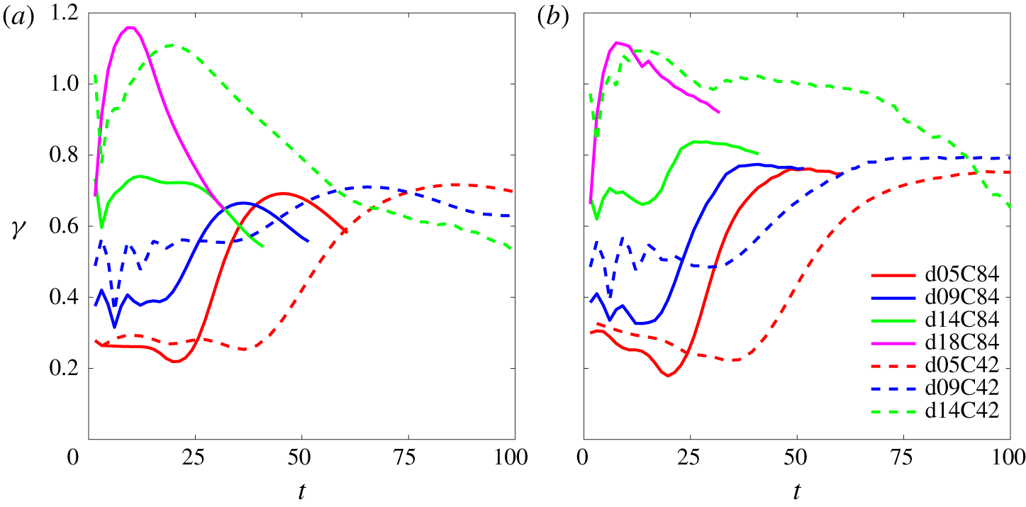
The time histories of  $\unicode[STIX]{x1D6FE}$ from our simulation results of cases with various particle sizes and two different
 $\unicode[STIX]{x1D719}_{0}^{\ast }$ are presented in figure 10. As shown in figure 10(a), in all cases except those with the relatively large particle size (cases d18C84 and d14C42),
 $\unicode[STIX]{x1D6FE}$ begins to increase from relatively small values, reaching a maximum value of approximately 0.70, and then decreases, despite certain fluctuations at the beginning (
 $t<10$) in some cases. Typically, the increases in
 $\unicode[STIX]{x1D6FE}$ in cases d05C84, d09C84, d14C84, d05C42 and d09C42 correspond to the onset of the DD convection in each case (see figure 7). The notable difference in
 $\unicode[STIX]{x1D6FE}$ in cases d18C84 and d14C42 is the sudden increase to slightly greater than 1. This is due to the rapid settling of individual particles, which soon leads to the formation of a thin layer of reversed buoyancy and the resulting buoyancy-dominant plumes. This, as discussed in § 3, differs from the pattern of the DD sedimentation in the other cases. After reaching the peak values,
 $\unicode[STIX]{x1D6FE}$ decreases when descending plumes begin to pass the lower bound of the thermally controlled region and reach the lower region of the domain in which the temperature gradient vanishes. As discussed in § 8, this decrease is due to significant horizontal motion (i.e. secondary instability) in this region. To focus on the thermally controlled region, figure 10(b) shows
 $\unicode[STIX]{x1D6FE}$ values sampled only within the thermally controlled region. It differs from figure 10(a) in that, except for cases d18C84 and d14C42, the
 $\unicode[STIX]{x1D6FE}$ values remain relatively steady after reaching their peaks. Our simulation shows that, as long as the sedimentation pattern is DD convection, this trend does not differ significantly between various particle sizes and initial concentrations. Except for slightly greater values in cases d14C84 and d09C42, the final values of
 $\unicode[STIX]{x1D6FE}$ in these cases are approximately 0.75, which is used as a constant value for
 $\unicode[STIX]{x1D6FE}$ in the thermally controlled region in the quasi-steady state.
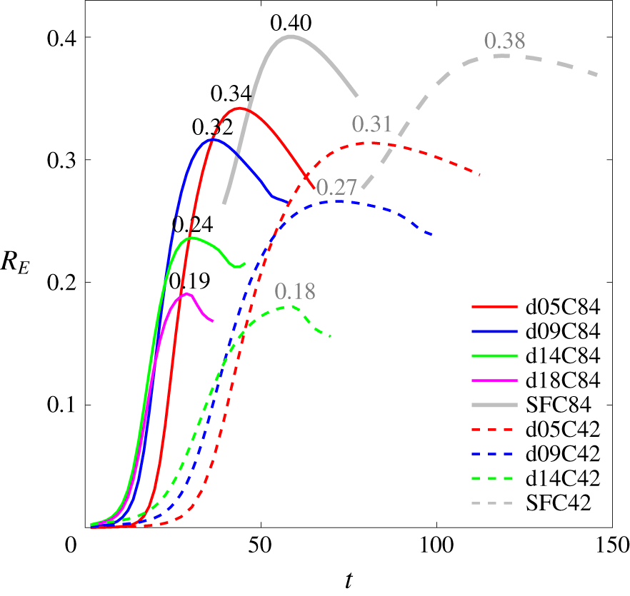
Time histories of the ratio  $R_{E}=-(\text{d}/\text{d}t)(\unicode[STIX]{x0394}PE_{T})/(\text{d}/\text{d}t)(\unicode[STIX]{x0394}PE_{p}-DD)$ in representative cases. Each number indicates the peak value of the associated curve.

The time histories of  $R_{E}$ from cases with various particle sizes and two different
 $\unicode[STIX]{x1D719}_{0}^{\ast }$ are presented in figure 11, along with the salt-finger cases for comparison. Values for
 $R_{E}$ typically begin to increase at the onset of the DD convection, reach a peak and then decrease. The peak values for all particle sizes range from 0.18 to 0.34. The peak value of
 $R_{E}$ increases as the particle size decreases. The decreased bulk thermal flux in cases with larger particles is due to the asymmetry of the vertical distribution of the temperature anomaly, as discussed in § 5. The peak value for the case of salt fingers with a high concentration reaches 0.4, which may be treated as a case in which
 $w_{s}$ asymptotically attains zero. Typically, given the same particle size, the case with a smaller particle concentration attains a slightly lower peak value in
 $R_{E}$ than its higher-concentration counterpart. This is because a lower particle concentration leads to slower development of fingers, such that it takes longer for
 $R_{E}$ to reach its peak than in the high-concentration case. In these cases, as the layer of the temperature gradient evolves over time due to diffusion (i.e.
 $\text{d}T_{r}/\text{d}z$ decreases with time), the capacity of the thermal contribution also decreases with time, such that the peak
 $R_{E}$ decreases as the initial particle concentration decreases.
With a constant value  $\unicode[STIX]{x1D6FE}=0.75$ (see figure 10) and values of
 $R_{E}$ from figure 11, one may examine the formula for the velocity scale, equation (6.18), for the quasi-steady state in the thermally controlled region in each case. To show this, we measure the vertical velocity component at the tips of all rising plumes at
 $z>0$. To make consistent velocity measurement in each case, we introduce a scalar field
 $\unicode[STIX]{x1D6F9}$ to indicate particle-laden and particle-free layers; i.e. when
 $t=0$,
 $$\begin{eqnarray}\unicode[STIX]{x1D6F9}=\left\{\begin{array}{@{}ll@{}}0\quad & \text{if }\unicode[STIX]{x1D719}^{\ast }=0,\\ 1\quad & \text{otherwise}.\end{array}\right.\end{eqnarray}$$
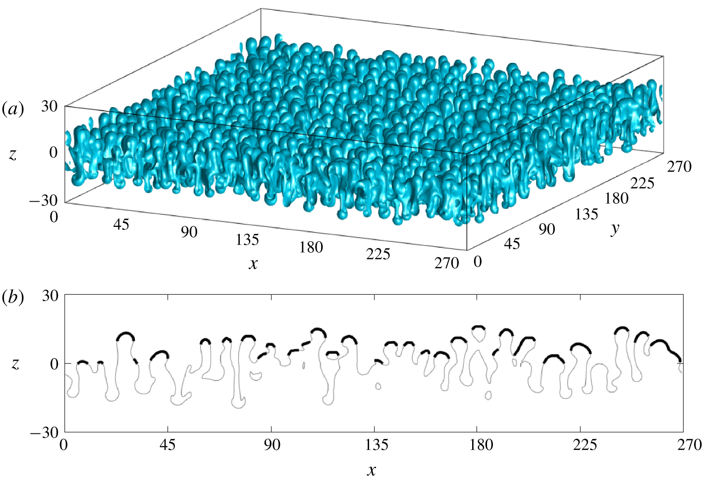
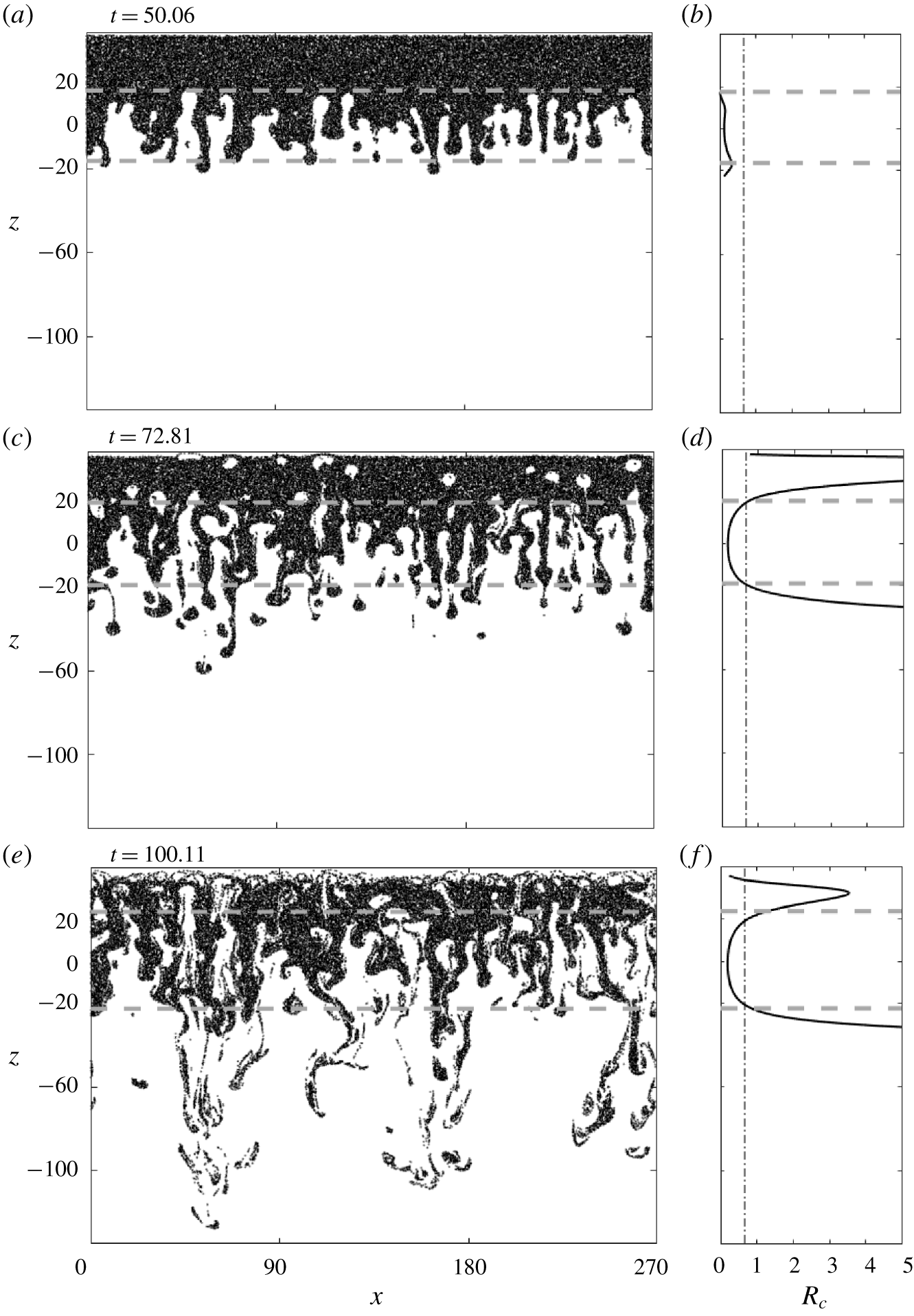
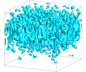
Its transport is then calculated by  $\text{D}\unicode[STIX]{x1D6F9}/\text{D}t=0$. Figure 12(a,b) shows an example of the iso-surface of
 $\unicode[STIX]{x1D6F9}=0.5$ at
 $t=50.06$ in case d05C84 and the associated contour line at the central slice in the
 $y$-direction, respectively. Velocities are then sampled at the tip area of the iso-surface of
 $\unicode[STIX]{x1D6F9}=0.5$ at
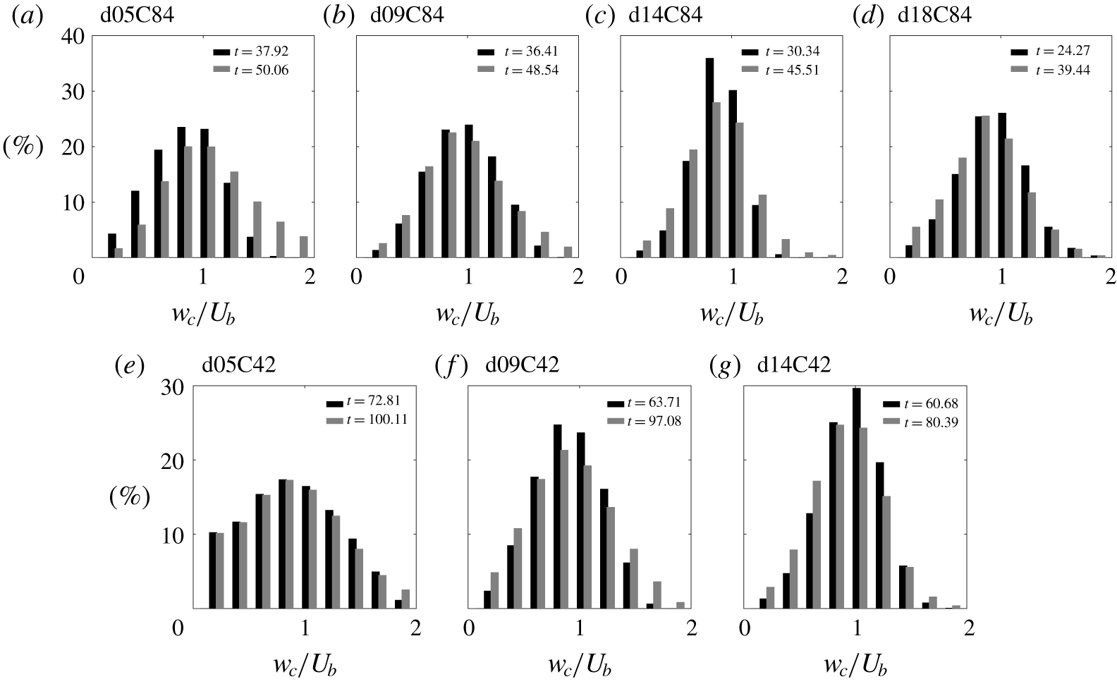
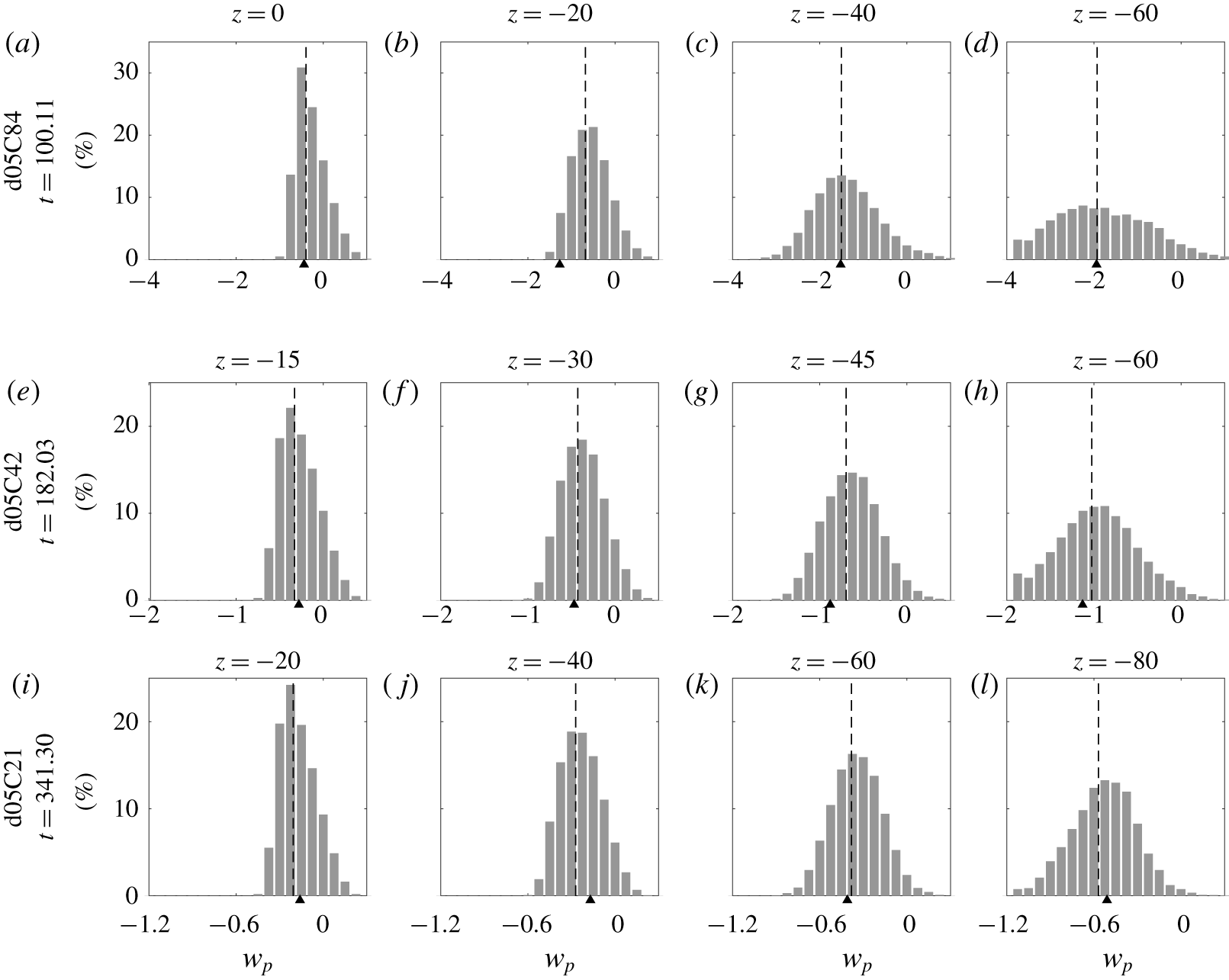
 $z>0$ that can be projected to a downward-facing horizontal plane at the top of the domain in each case, as marked by the black thick lines in figure 12(b). Figure 13 shows histograms of the measured vertical velocity component, normalized by
 $U_{b}$, at two instants in representative cases. In each case of figure 13, the two representative time instants are chosen based on the duration for which a quasi-steady development of the uprising fingers within the thermally controlled region is observed. Figure 13 shows that
 $w_{c}/U_{b}=1$ is fairly close to the peak values of the histogram in all cases, indicating that
 $U_{b}\sim 0.75(1-R_{E})/R_{\unicode[STIX]{x1D70C}}$ (in which
 $R_{E}$ is obtained from the peak value in figure 11), seems to be a proper scaling for the plume velocity at the quasi-steady state.


Histograms of the percentage of the vertical velocity of rising plumes normalized by  $U_{b}$ sampled at the tips of the rising plumes (see figure 12) at two representative time steps during the quasi-steady state in the DD regime in cases d05C84, d09C84, d14C84, d18C84, d05C42, d09C42 and d14C42.

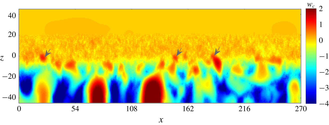
Snapshot of vertical velocity corresponding to figure 2(f) to show certain residual uprising particle-free bubbles, indicated by grey arrows, in the case of an intermediate pattern of sedimentation (d18C84).

7 Criterion of double-diffusive sedimentation
The velocity scale  $U_{b}=\unicode[STIX]{x1D6FE}(1-R_{E})/R_{\unicode[STIX]{x1D70C}}$ characterizes the quasi-steady velocity for which the DD sedimentation can reach with the given conditions, including particle size, buoyancy and thermal conditions. Thus, for the flow field at the tips of the rising plumes, replacing
 $U_{b}\hat{\boldsymbol{e}}_{3}$ with
 $\boldsymbol{u}_{c\mid p}$ in (2.13) and assuming a sufficiently small particle size for which
 $St\ll 1$, (2.13) can be reduced to an equation that describes the particles’ dominant vertical motion, which reads
 $$\begin{eqnarray}w_{p}\sim U_{b}-w_{s}.\end{eqnarray}$$
That is, the motion of the particles at the tips of the rising plumes is simply a balance between the gravitational settling and the hydrodynamic force resulting from DD convection. For particles that are in equilibrium with the flow motion, the resulting particle velocity is just the difference between the characteristic hydrodynamic velocity and the settling velocity. That is, if  $w_{p}>0$ in (7.1), particle-free fingers consistently move upward, and the sedimentation pattern is more symmetrical (but can never be, as
 $w_{s}\neq 0$) about
 $z=0$, resulting in a permanent pattern of DD convection. Otherwise, although DD instability can still occur within a very short time, the uprising motion of the fingers ceases near the particle-laden interface because the plume velocity cannot compensate for the gravitational settling of particles. However, there is no clear cut result between the two sedimentation patterns, and in (7.1), if
 $w_{p}\approx 0$, one would expect settling-driven RTI accompanied with certain uprising particle-free bubbles at the interfacial region, which appears in our cases d18C84 and d14C42. As shown by figure 14, which presents a snapshot of the vertical velocity corresponding to figure 2(f), certain insignificant rising bubbles can be found from the spots (see arrows) of the positive velocity at the interfacial region. It is also noted that
 $U_{b}$ increases as the particle size increases due to the decrease in
 $R_{E}$. As shown in figure 11, the peak
 $R_{E}$ of the two intermediate cases, d18C84 and d14C42, are less than
 $0.20$. Therefore, one may simply substitute
 $R_{E}=0.20$ and
 $\unicode[STIX]{x1D6FE}=0.75$ (see discussion of § 6) in (6.17) to obtain a velocity scale
 $U_{R}$ for the intermediate pattern, i.e.
 $$\begin{eqnarray}U_{R}^{\ast }={\displaystyle \frac{0.60}{R_{\unicode[STIX]{x1D70C}}}}U,\end{eqnarray}$$
or its non-dimensional form
 $$\begin{eqnarray}U_{R}={\displaystyle \frac{0.60}{R_{\unicode[STIX]{x1D70C}}}}.\end{eqnarray}$$
Based on (7.3), a velocity ratio
 $$\begin{eqnarray}R_{v}={\displaystyle \frac{w_{s}}{U_{R}}}=1.67R_{\unicode[STIX]{x1D70C}}w_{s}\end{eqnarray}$$
characterizes the vertical motion of particles at tips of rising plumes, which serves as a criterion to distinguish the occurrence of two sedimentation patterns: DD convection and settling-driven RTI.
It is worthwhile to compare the present criterion  $R_{v}$ with the one suggested by Burns & Meiburg (Reference Burns and Meiburg2012). In their theoretical analysis, the authors introduced a thickness ratio
 $$\begin{eqnarray}R_{t}={\displaystyle \frac{w_{s}t}{l_{s}}},\end{eqnarray}$$
where  $l_{s}$ is the thickness of the region of the background salinity (temperature) gradient. They showed that instabilities tend to be RTI when
 $R_{t}>1$ and become double diffusion for
 $R_{t}<1$. A critical condition in their analysis was that the particle-laden layer is initially associated with the same order of magnitude of the mixing zone’s thickness as that of the background salinity field. In contrast, the present particle-laden layer is associated with a sharp interface, such that the initial layer of the temperature gradient is infinitely thick. Therefore, within a short period, this study is analogous to the case with
 $R_{t}\ll 1$ in Burns & Meiburg (Reference Burns and Meiburg2012) for which DD sedimentation would occur. However, an issue arises when using (7.5) in that
 $R_{t}$ increases over time, such that RTI will always occur after a long time. This is a consequence of the linear stability analysis in which the subsequent quasi-steady state of the real flow is not considered. It is thus suggested to replace
 $t$ with a time scale such that
 $R_{t}$ would not grow without bound. Next, it is reasonable to assume this time scale to be the time necessary for a finger to flow through the region of the background density gradient (i.e.
 $l_{s}/U_{b}$). Replacing
 $t$ with
 $l_{s}/U_{b}$ in (7.5) results in the same formula as the present velocity criterion
 $R_{v}$.
Figure 15 presents  $w_{s}$ and
 $U_{R}$ from the datasets of existing laboratory studies, including Hoyal et al. (Reference Hoyal, Bursik and Atkinson1999a,Reference Hoyal, Bursik and Atkinsonb), Parsons & Garcia (Reference Parsons and Garcia2000), Parsons et al. (Reference Parsons, Bush and Syvitski2001), Houk & Green (Reference Houk and Green1973), Green & Schettle (Reference Green and Schettle1986), Green (Reference Green1987), Chen (Reference Chen1997), Davarpanah & Wells (Reference Davarpanah and Wells2016), Rouhnia & Strom (Reference Rouhnia and Strom2015), the numerical results of Shao et al. (Reference Shao, Hung and Chou2017) and our study. Blue, green and red are used to indicate the DD, intermediate and settling-driven RTI patterns in figure 15. These referenced studies focused either on DD sedimentation or settling-driven RTI, so it is easy to distinguish the sedimentation patterns from these studies. In the laboratory set-up, observation begins after slowly removing a plate with a thickness
 $\unicode[STIX]{x1D6FF}_{e}$ that originally separates the two layers of fluids in a tank, during which a rapid mixing of the background temperature or salinity can be expected. Because the measured data of the temperature (or salinity) gradient are not available, here, we assume an error-function profile as in (2.23), in which
 $h_{0}=0.86\unicode[STIX]{x1D6FF}_{e}$, such that the temperature (salinity) at the point originally located at the top edge of the plate is equal to 0.9
 $T_{r,up}$. Approximated gradients in the laboratory experiments are then obtained by calculating the value at
 $z=0$ of the first derivative to the error-function profile. The values of important parameters of each data point in figure 15 are summarized in Appendix B. Figure 15 shows that
 $R_{v}=1$ (shown by the dashed line) seems to be a good indicator to distinguish various patterns (as marked in various colours), although misprediction can be found at very few data points, one from Rouhnia & Strom (Reference Rouhnia and Strom2015) and another from Davarpanah & Wells (Reference Davarpanah and Wells2016), when
 $R_{v}\approx 1$. It is anticipated that both patterns can be observed when
 $w_{s}\approx U_{R}$. Because the ‘intermediate’ pattern is usually not defined in these experimental studies, depending on the method of observation, the pattern could be interpreted as either DD convection or settling-driven RTI in the laboratory experiment. It should also be noted that uncertainties may arise from our approximation for the temperature gradient in the laboratory using the error function, which can also lead to failure of prediction.
Plot of  $w_{s}$ and
 $U_{R}$. Data are collected from the experimental results of each reference and the simulated result of our study and Shao et al. (Reference Shao, Hung and Chou2017). The dashed line indicates
 $w_{s}=U_{R}$. Red, green and blue are used to indicates settling-driven RTI, intermediate and DD convection, respectively. The details of data points from this study are summarized in table 1, and those from previous studies are listed in appendix B.

It should be noted that, here, to demonstrate the applicability of  $R_{v}$, we run additional cases using the diffusivity of salinity,
 $\unicode[STIX]{x1D705}_{S}=1.5\times 10^{-9}~\text{m}^{2}~\text{s}^{-1}$, as the diffusivity of the agent for background stratification. Three particle diameters,
 $d_{0}=1$,
 $2$ and
 $9~\unicode[STIX]{x03BC}\text{m}$ are used. For the first two cases with small particles, to avoid high computational loading, we use the single-phase approach (also known as the equilibrium Eulerian approach (Yu et al. Reference Yu, Hsu and Balachandar2014; Burns & Meiburg Reference Burns and Meiburg2015)) to model the transport of the particle concentration. It solves the advection–diffusion equation along with vertical transport due to the settling velocity. We use the particle diffusivity
 $\unicode[STIX]{x1D705}_{\unicode[STIX]{x1D719}}=10^{-10}~\text{m}^{2}~\text{s}^{-1}$, which is approximately the lowest value our model can achieve because the order of magnitude of the numerical diffusivity is
 $10^{-11}~\text{m}^{2}~\text{s}^{-1}$ given by the grid resolution in our simulation. As shown in table 1, these cases are named d01C84Ssp, d02C84Ssp and d09C84S for
 $d_{0}=1$,
 $2$ and
 $9~\unicode[STIX]{x03BC}\text{m}$, respectively, in which ‘S’ stands for salt and ‘sp’ means the single-phase simulation. Figure 16 presents representative snapshots of
 $\unicode[STIX]{x1D719}$ for case d02C84Ssp and particles for case d09C84S. It shows a clear difference between the two cases in that case d02C84Ssp exhibits strong symmetry about
 $z=0$ (see figure 14a), whereas case d09C84S shows sheet-like plumes formed below the interface with significantly greater wavelengths. The former pattern corresponds to DD sedimentation, and the latter is the pattern during the dissipation stage of settling-driven RTI, also known as leaking, a detailed discussion of which can be found in Shao et al. (Reference Shao, Hung and Chou2017).
Representative snapshots of  $\unicode[STIX]{x1D719}$ in case d02C84Ssp and particles in cases d09C84S (b) using the diffusivity of salinity,
 $\unicode[STIX]{x1D705}_{S}=1.5\times 10^{-9}~\text{m}^{2}~\text{s}^{-1}$, as the diffusivity of the agent for background stratification. The resulting values for the length scale using the
 $\unicode[STIX]{x1D705}_{S}$ value is
 $L=7.03\times 10^{-5}~\text{m}$, which is used as the unit in this figure.

Snapshots of particles at the central slice (a,c,e) in the  $y$-direction at representative time points in case d05C84 along with corresponding profiles of
 $R_{c}$ (b,d,f). Grey dashed lines indicate locations where
 $T_{r}=T_{r,low}+0.1(T_{r,up}-T_{r,low})$ (bottom line) and
 $T_{r}=T_{r,low}+0.9(T_{r,up}-T_{r,low})$ (top line), which are used to indicate the locations of the plume relative to the gradient of the background temperature. The dash-dotted lines in (b,d,f) indicate
 $R_{c}=0.67$, at which secondary instability occurs. In these panels, point markers are used to represent the positions of the particles located in
 $L_{y}/2-0.1\unicode[STIX]{x1D6FF}y\leqslant y\leqslant L_{y}/2$, in which
 $L_{y}$ is the domain size in the
 $y$-direction and
 $\unicode[STIX]{x1D6FF}y$ is the grid size in the
 $y$-direction.

8 Secondary instability
The discussion has thus far focused on sedimentation in the thermally controlled region. However, when the thermal effect weakens, secondary instability occurs in the form of strong horizontal motion, which is also known as collective instability. Theoretical arguments regarding collective instability in the context of DD salt fingers were first made by Stern (Reference Stern1969) and further refined by Holyer (Reference Holyer1981, Reference Holyer1984, Reference Holyer1985). Holyer (Reference Holyer1985) rigorously showed that instability occurs when  $R_{c,S}>0.67$ in the three-dimensional case, recalling that
 $R_{c,S}$ is the ratio between the total convective flux to the conductive flux (see (4.3)). In the case of suspended particles, the negligible conductive flux for particles due to negligible diffusivity (i.e. (4.7)) may result in greater possibilities for the occurrence of collective instability. Because collective instability only occurs in the DD case, here we focus on cases with small particles, i.e.
 $d_{0}=5~\unicode[STIX]{x03BC}\text{m}$. Figure 17 shows a series of representative snapshots of particles at the central slice in the
 $y$-direction along with profiles of corresponding
 $R_{c}$. Figure 17(a) represents the quasi-steady fingers in the thermally dominant regime moving dominantly in the vertical direction, and
 $R_{c}<0.67$ in figure 17(b) indicates a stable flow regime at this time point. Figure 17(c) shows particle-laden fingers at the onset of secondary instability, during which
 $R_{c}$ begins to exceed 0.67 at approximately
 $z<-20$ in the lower half of the domain, as shown in figure 17(d). At this stage, despite slight horizontal distortion of the finger tips, slight variation in the direction of finger motion does not show significant flow instabilities. However, as shown by the histograms of the magnitudes of the horizontal velocity components,
 $U_{h}=\sqrt{u_{c}^{2}+v_{c}^{2}}$, sampled at three horizontal planes near
 $z=-20$ in figure 18(d), the significant increase in
 $U_{h}$ below
 $z=-20$ indicates that plumes are susceptible to disturbances in the horizontal direction. As shown in figure 18(a–c), the distributions of particles become less homogeneous upon the occurrence of instability (see figure 18b,c) compared with those before the occurrence of instability (figure 18a). As with typical collective instabilities, such horizontal disturbances are associated with long wavelengths (Stern Reference Stern1969; Holyer Reference Holyer1981). Fingers are collected to a few groups at the later time stage, as shown in figure 17(e). At this time, as shown in figure 18(h), the horizontal flow motion becomes stronger than that during the onset of instability (see figure 18d). As shown in figure 18(f,g), the plumes are elongated in the horizontal direction. Compared with the location before the occurrence of the secondary instability as shown in figure 18(e), plumes become more sheet like, and the distribution exhibits a strong lack of homogeneity below
 $z=-20$ due to the secondary instability.
Snapshots of plan view (a–c,e–g) of particles at representative vertical points at  $t=72.81$ (a–c) and
 $100.11$ (e–g) along with the corresponding histograms (d,h) of horizontal speed
 $U_{h}$ sampled in each grid cells.

Spectra of horizontal distributions of the volume fraction  $\unicode[STIX]{x1D719}$ in cases d05C84, d05C42 and d05C21 at representative vertical levels and time steps during which secondary instability develops and the corresponding vertical profiles of
 $R_{c}$. Numbers in (a,c,e) indicate wavenumbers of dominant modes,
 $k_{0}$, for each spectrum, (i.e. the associated wavenumber for the peak
 $\hat{\unicode[STIX]{x1D719}}(k)$ of each spectrum). The dash-dotted lines in (b,d,f) indicate
 $R_{c}=0.67$, at which secondary instability occurs.

An important characteristic of the secondary instability is the change of the dominant mode of particle plumes from the DD regime to the collective instability. Because the latter is susceptible to long-wave disturbances in the horizontal direction, it is anticipated that the resulting grouping and merging of plumes reflect the length scale of the long-wave disturbance. Following the theoretical analysis by Holyer (Reference Holyer1981), one can obtain the dispersion relationship of the long-wave disturbance of the collective instability as a function of  $R_{f}$ (4.6) and the diffusivity ratio
 $R_{\unicode[STIX]{x1D705}}$; details are provided in appendix C. In our cases,
 $R_{f}$ is typically less than
 $0.4$ (see figure 5), and in the lower region of the domain in which the secondary instabilities occur,
 $R_{f}$ usually ranges from
 $0.10$ to
 $0.20$. According to appendix C, with an infinitesimal diffusivity for concentrations of particles, the most unstable modes, denoted as
 $k_{0}$, in this
 $R_{f}$ regime range from
 $0.09$ to
 $0.15$, and the growth rates are associated with slow variation with
 $k$. Therefore, one may simply take
 $k_{0}\sim 0.1$ as a scaling for our cases. This can be confirmed by figure 19, in which we show the spectra of horizontal distributions of the volume fraction
 $\unicode[STIX]{x1D719}$ in cases d05C84, d05C42 and d05C21 at representative vertical levels and the time steps during which the secondary instability develops and the corresponding vertical profiles of
 $R_{c}$. Figure 19 shows that in all cases of various initial particle concentrations, the dominant modes of the horizontal distribution of
 $\unicode[STIX]{x1D719}$ shift to significantly lower values once
 $R_{c}$ is roughly greater than
 $0.67$. The final lower value of
 $k_{0}\sim 0.1$, which is independent of the initial concentration of particles, is consistent with the linear theory (see appendix C).
8.1 Enhanced particle settling: a simple scaling argument
Due to the resulting convective motion, the sedimentation of particles can be significantly enhanced relative to that induced by gravity exerted on a single particle (i.e. Stokes settling). In our cases, the vertical velocities inside the plumes are well scaled with  $U_{b}^{\ast }$ (6.17) in the thermally controlled region but can be enhanced when secondary instability occurs. In what follows, we provide a simple argument for the estimation of the further enhancement of particle settling due to secondary instability.
Schematic plots to show the horizontal distributions of plumes in the thermally controlled region in which the DD convection occurs (a) and in the region below the level at which secondary instability occurs (b) for the case of  $M=4$ (see (8.2)). In panel (b), we assume full anisotropy for plumes’ geometry in the horizontal direction after the occurrence of secondary instability. The arrows in (b) indicate horizontal flow motions resulting from secondary instability. The shaded regions represent particle-laden plumes.

Histograms for the percentage of the particle number versus the vertical velocity component of particles,  $w_{p}$, sampled at vertical levels corresponding to those in the spectrum plots shown in figure 19(a,c,e), along with the predicted particle velocities, marked with black triangles, in each case using either the scaling argument
 $w_{p}\sim U_{b}+w_{s}$ for the thermal dominant regime (a,e,i) or (8.3) with
 $f=1$ and dominant modes (
 $k_{0}$) obtained from figure 19(a,c,e) in the secondary-instability regime (b–d, f–h and j–l). Black dashed lines indicate the mean value for each histogram. In each histogram, for a specified vertical level at
 $z=z_{s}$, the velocities are sampled for particles within
 $z_{s}\pm 0.5\unicode[STIX]{x1D6FF}z$, in which
 $\unicode[STIX]{x1D6FF}z$ is the vertical grid size.

First, it is observed that the distribution of plumes resulting from DD convection is fairly homogeneous in the horizontal direction (see figure 18a,e) and symmetrical in the vertical. That is, the sizes of the upward-moving plumes are identical to those of the downward-moving plumes, such that the total cross-sectional area in the horizontal plane of the particle-laden plumes, denoted with  $A_{p,DD}$, is equal to that of the ambient particle-free fluid, denoted with
 $A_{c,DD}$, as illustrated in figure 20(a). That is,
 $$\begin{eqnarray}A_{p,DD}=A_{c,DD}={\textstyle \frac{1}{2}}A_{tot},\end{eqnarray}$$
where the subscript  $DD$ denotes the double-diffusion regime and
 $A_{tot}$ is the total area of the horizontal plan of the domain. In the secondary-instability region, the dominant wavelength of the distribution of plumes is then increased by a multiple
 $M$. The increase in the dominant wavelength is caused by the increase in the length scale of the cross-section of the clear-fluid region on the horizontal plane, as seen in figure 18(e–g), due to long-wave disturbances and subsequent convection. In this flow regime, as shown by the plan view in figure 18(g), patches of particle-free regions are approximately isotropic in the horizontal direction while those of particle-laden plumes exhibit strong anisotropy in a way that plumes are greatly elongated in one horizontal direction. Therefore, it may be reasonable to assume that the horizontal length of the plume, denoted as
 $\unicode[STIX]{x1D706}_{p1,SI}$, is retained as in the DD regime in one horizontal dimension, but in the other horizontal dimension, the length scale, denoted as
 $\unicode[STIX]{x1D706}_{p2,SI}$, increases by a multiple
 $fM$, where
 $M=k_{0,DD}/k_{0,SI}$ is the ratio of the dominant mode of the horizontal distribution of particles between the DD and secondary instability regimes, and
 $f$, varying from
 $1/M$ to
 $1$, is an index of the plumes’ horizontal anisotropy (i.e. isotropic if
 $f=1/M$ and otherwise if
 $f=1$). As illustrated in figure 20(b), using
 $f=1$ by assuming full anisotropy for plumes’ geometry in the horizontal direction gives
 $$\begin{eqnarray}A_{p,SI}={\displaystyle \frac{M}{M^{2}}}A_{c,SI}={\displaystyle \frac{1}{M+1}}A_{tot}.\end{eqnarray}$$
Based on mass conservation (i.e. constant flux in the vertical direction), equations (8.1) and (8.2) give an estimation of the increase in plumes’ vertical speeds,  $W_{p}$, as
 $$\begin{eqnarray}R_{W}={\displaystyle \frac{W_{p,SI}}{W_{p,DD}}}={\displaystyle \frac{M+1}{2}}.\end{eqnarray}$$
Figure 21 presents histograms of particle numbers (in percentage) versus the vertical velocity component of particles,  $w_{p}$, sampled at vertical levels corresponding to those in the spectrum plots shown in figure 19(a,c,e), along with the predicted particle velocities using (8.3) and dominant modes (
 $k_{0}$) obtained from figure 19(a,c,e). As previously mentioned in § 6 within the thermally controlled region, DD convection dominates, and the speeds of the plumes scale with
 $U_{b}$. Therefore, the downward speeds of the particles in the DD regime are predicted using
 $U_{b}+w_{s}$, in which we simply use
 $R_{E}=0.30$ according to cases with
 $d_{0}=5~\unicode[STIX]{x03BC}\text{m}$ shown in figure 11, such that
 $U_{b}=0.53$ according to (6.18). As marked by black triangles in figure 21(a,e,i), the predicted values are fairly close to the mean value of
 $w_{p}$ (highlighted by dashed lines) and seem to be a good scaling law for particle velocity in the DD regime. Moreover, at vertical levels below the point at which the secondary instability occurs, figure 21(c,d,f–h,j–l) also shows that the values predicted using (8.3) are close to the mean values of the sampled particle velocity. The overprediction found in figure 21(b) is because
 $z=-20$ lies almost exactly upon the point of the onset of secondary instability (see figure 19b), at which plumes are typically subject to a transition from large modes of
 $k_{0}$ in DD regime to small
 $k_{0}$ in the secondary-instability regime. In the transition, distributions of
 $\unicode[STIX]{x1D719}$ can exhibit a wider band width in their dominant modes. For example, as shown by the spectrum in figure 19(a), another peak
 $\hat{\unicode[STIX]{x1D719}}(k)$ only slightly less than the value associated with
 $k_{0}$ (
 $=0.12$) can also be found at
 $k=0.23$ (as shown by the value in parentheses in figure 19a). When this range of
 $k_{0}$ is considered (i.e.
 $k_{0}=0.12$–
 $0.23$), the prediction in figure 21 can be much improved.
Although here we show that the further enhancement of particle speeds can be estimated from the change in the total cross-sectional areas of the plumes on each horizontal plane, it seems impossible to predict the size and distribution of plumes in the secondary-instability regime due to the strong nonlinear effect. However, one may use the dominant wavenumber predicted by the linear theory (e.g. Holyer Reference Holyer1981) as a threshold value of  $k_{0}$ in this flow regime, as given by appendix C. It is thus possible to estimate the minimum settling enhancement for individual particles.
9 Concluding remarks
This study involved a series of numerical simulations conducted to examine DD sedimentation in stratified background flows. For small particles, our simulation shows the growth of fingers at the interfacial area that are similar to DD salt fingers. When the particles becomes larger, the rising motion of particle-free fingers is suppressed due to the particle’s settling velocity, and our simulation shows the pattern of settling-driven RTI. In these cases, the maximum settling enhancement ( $SE$) reaches about six times that induced by individual particle settling and then decreases as the particles become larger. Moreover, for cases of DD sedimentation, our simulation results show very little variation in the temperature-to-particle flux ratio
 $R_{f}$ in cases with different particle sizes and initial concentrations, which is consistent with previous theoretical derivations and experimental observations. The constant
 $R_{f}$ then gives the scaling law for the fluctuation flux
 $\overline{w^{\ast \prime }\unicode[STIX]{x1D719}^{\ast \prime }}\sim \unicode[STIX]{x1D719}_{0}^{\ast 2}$, which is consistent with the existing theoretical results for the quasi-steady, fully vertical fingers.
An analysis of the energy budget is then conducted to show that the settling enhancement is mainly due to a combination of the thermal effect and shear dissipation. Moreover, the analysis showed that the contribution of the thermal effect to the settling enhancement decreases when the particle size increases. Based on the balance of the temporal evolution of the energy budget, we then derived an expression for final velocity scaling  $U_{b}$ as a function of the density ratio
 $R_{\unicode[STIX]{x1D70C}}$, the ratio
 $R_{E}$ (6.11) and
 $\unicode[STIX]{x1D6FE}$ that represents the proportion of the momentum associated with particle-laden plumes to half of the total momentum of the bulk flow (6.16). While the simulation set-up gives values for
 $R_{\unicode[STIX]{x1D70C}}$, adopting values for
 $R_{E}$ and
 $\unicode[STIX]{x1D6FE}$ from our simulation results enables proper scaling for the final speed of the plumes in each simulation case. Moreover, according to the simulation results, we use the marginal case with
 $R_{E}=0.2$ to obtain a velocity criterion to predict the occurrence of either DD sedimentation or settling-driven RTI. Several previous experimental results are compared with our proposed criterion and shows good agreement for the prediction of sedimentation patterns.
In addition to the thermally controlled region, we investigate changes in the particle-laden plumes below the region of the apparent temperature gradient. In this region, due to the vanishing temperature gradient and thus the associated conductive flux, secondary instability occurs in the form of significant horizontal flow motion. Our simulation results show that the resulting initial shift of the dominant modes can be approximated by the existing theoretical analysis on collective instabilities for salt fingers. Finally, we present a simple scaling argument for a change in the total cross-sectional area of particle-laden plumes, which is then used to scale the resulting enhanced sedimentation for individual particles.
Using Eulerian–Lagrangian simulation, this study presents a systematic examination of convective sedimentation in stratified flows. Its main purpose is to reveal important bulk properties associated with DD sedimentation. The velocity scaling derived from the energy budget analysis characterizes the associated flow velocity in the thermally controlled region in the quasi-steady state. This is critical to the assessment of the resulting enhancement of particle settling and in distinguishing sedimentation patterns. Moreover, we show the importance of secondary instability in DD sedimentation, and our analysis of the secondary-instability regime adds to our understanding of the final enhancement of the sedimentation rate.
Acknowledgements
We gratefully acknowledge the support of the Taiwan Ministry of Science and Technology (MOST) Civil and Hydraulic Engineering Program under grant no. MOST 106-2628-E-002-016-MY4, the Ministry of Education (MOE) Higher Education Sprout Project in Taiwan (NTU Core Consortium: 108L880206) and National Taiwan University career development project (NTU-CDP-108L7720). We also thank the reviewer, Professor J. McElwaine, for pointing out the issue of non-physical particle clustering in our explicit particle tracking scheme. The computation was performed on the Dell PowerEdge M620 supercomputer cluster located at Taida Institute of Mathematical Science at National Taiwan University, which is gratefully acknowledged.
Declaration of interests
The authors report no conflict of interest.
Appendix A
Consider solving the motion of a single particle subject to a purely rotational motion of fluid,  $(u,v)=(\unicode[STIX]{x1D6E4}y,-\unicode[STIX]{x1D6E4}x)$. Using the explicit Euler method with the time step
 $\unicode[STIX]{x1D6FF}_{t}$, the equations that update the particle motion at the time step
 $n+1$ can be written as
 $$\begin{eqnarray}\left.\begin{array}{@{}c@{}}x^{(n+1)}=x^{(n)}+\unicode[STIX]{x1D6FF}_{t}\unicode[STIX]{x1D6E4}y^{n},\\ y^{(n+1)}=y^{(n)}-\unicode[STIX]{x1D6FF}_{t}\unicode[STIX]{x1D6E4}x^{n}.\end{array}\right\}\end{eqnarray}$$
The solution for (A 1) can be written as
 $$\begin{eqnarray}\left.\begin{array}{@{}c@{}}x^{(n+1)}=\text{Re}[C^{(n)}(1+\text{i}\unicode[STIX]{x1D6FF}_{t}\unicode[STIX]{x1D6E4})],\\ y^{(n+1)}=-\text{Im}[C^{(n)}(1+\text{i}\unicode[STIX]{x1D6FF}_{t}\unicode[STIX]{x1D6E4})],\end{array}\right\}\end{eqnarray}$$
where  $C^{(n)}=x^{(n)}-\text{i}y^{(n)}$. Based on (A 2), the radius of the particle trajectory,
 $r^{(n)}$, can be obtained with
 $$\begin{eqnarray}\displaystyle r^{(n)}=\sqrt{x^{(n)2}+y^{(n)2}} & = & \displaystyle |C^{(0)}|(1+\unicode[STIX]{x1D6FF}_{t}^{2}\unicode[STIX]{x1D6E4}^{2})^{n/2}\nonumber\\ \displaystyle & {\approx} & \displaystyle |C^{(0)}|\exp \left({\displaystyle \frac{\widetilde{\unicode[STIX]{x1D70F}}\unicode[STIX]{x1D6FF}_{t}\unicode[STIX]{x1D6E4}^{2}}{2}}\right),\end{eqnarray}$$
where  $\widetilde{\unicode[STIX]{x1D70F}}=n\unicode[STIX]{x1D6FF}_{t}$ is a time scale of interest. Equation (A 3) shows that in the simulation, the particle can non-physically spiral outwards such that the radius of its trajectory increases. This is due to the numerical instability associated with the explicit Euler method while solving for problems with purely imaginary eigenvalues. This numerical error can be insignificant only if
 $\widetilde{\unicode[STIX]{x1D70F}}\unicode[STIX]{x1D6FF}_{t}\unicode[STIX]{x1D6E4}^{2}\ll 1$. In this study, using the largest value of the off-diagonal component of the strain-rate tensor to scale
 $\unicode[STIX]{x1D6E4}$, as shown in figure 22, one obtains
 $\unicode[STIX]{x1D6E4}\sim 0.8$. Also, we adopt a small computational time step
 $\unicode[STIX]{x1D6FF}_{t}=0.003$ such that particles can only move between two adjacent computational cells at each time step (Chou et al. Reference Chou, Gu and Shao2015). For a double-diffusion time scale
 $\widetilde{\unicode[STIX]{x1D70F}}=1$, this gives
 $\widetilde{\unicode[STIX]{x1D70F}}\unicode[STIX]{x1D6FF}_{t}\unicode[STIX]{x1D6E4}^{2}\sim 10^{-3}\ll 1$, such that the increase in the radius of the particle trajectory can be insignificant.
Snapshots of  $\unicode[STIX]{x2202}u/\unicode[STIX]{x2202}z$ (a) and
 $\unicode[STIX]{x2202}w/\unicode[STIX]{x2202}x$ (b) corresponding to figure 17(e), which is an example to demonstrate the values of the off-diagonal elements of the strain-rate tensor at the later stage when flows are relatively vigorous. Because the flow is fairly homogeneous in the horizontal plane, it is sufficient to show only
 $\unicode[STIX]{x2202}u/\unicode[STIX]{x2202}z$ and
 $\unicode[STIX]{x2202}w/\unicode[STIX]{x2202}x$ to obtain the scaling for
 $\unicode[STIX]{x1D6E4}$.

Appendix B
In this appendix, we summarize all data points plotted in figure 15 obtained from previous studies in table 2.
Summary of the experimental results of Houk & Green (Reference Houk and Green1973), Green & Schettle (Reference Green and Schettle1986), Green (Reference Green1987), Hoyal et al. (Reference Hoyal, Bursik and Atkinson1999a), Hoyal et al. (Reference Hoyal, Bursik and Atkinson1999b), Parsons & Garcia (Reference Parsons and Garcia2000), Rouhnia & Strom (Reference Rouhnia and Strom2015), Davarpanah & Wells (Reference Davarpanah and Wells2016) and Shao et al. (Reference Shao, Hung and Chou2017).
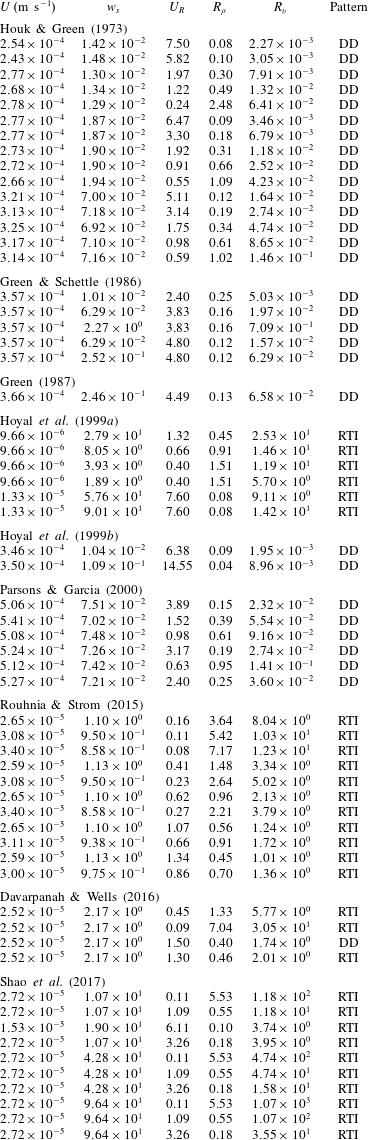
Appendix C
To obtain the dispersion relationship of the collective instability for the present cases, we solve the algebraic equations derived from the linear stability analysis in Holyer (Reference Holyer1981). In that analysis, the physical field, denoted as  $\unicode[STIX]{x1D6F9}(\boldsymbol{x})$, is written as
 $$\begin{eqnarray}\unicode[STIX]{x1D6F9}(\boldsymbol{x})=\unicode[STIX]{x1D6F9}_{m}(\boldsymbol{x})+\unicode[STIX]{x1D6F9}_{r}(\boldsymbol{x}),\end{eqnarray}$$
where subscripts  $m$ and
 $r$ denote the mean and rapidly varying parts, respectively. For the mean part, we seek solutions of the forms
 $$\begin{eqnarray}\unicode[STIX]{x1D6F9}_{m}=\left(\begin{array}{@{}c@{}}\unicode[STIX]{x1D713}_{m}\\ T_{m}\\ \unicode[STIX]{x1D719}_{m}\end{array}\right)={\mathcal{R}}\left(\left(\begin{array}{@{}c@{}}A\\ -\text{i}B\\ -\text{i}C\end{array}\right)\exp (\text{i}kx+\text{i}mz+\unicode[STIX]{x1D70E}t)\right).\end{eqnarray}$$
The wavenumber is given by  $\unicode[STIX]{x1D702}$, where
 $\unicode[STIX]{x1D702}^{2}=k^{2}+m^{2}$. The basic flow has
 $\unicode[STIX]{x1D707}\ll 1$. Without showing the detailed derivation in Holyer (Reference Holyer1981), the final algebraic equations to be solved are
 $$\begin{eqnarray}\displaystyle & \displaystyle -\left({\displaystyle \frac{\unicode[STIX]{x1D70E}}{Pr}}+\unicode[STIX]{x1D702}_{-}^{2}\right)\unicode[STIX]{x1D702}_{-}^{2}A_{1}+(1-k)(Ra_{T}B_{1}-Ra_{\unicode[STIX]{x1D719}}C_{1})=-{\displaystyle \frac{\text{i}m\widehat{W}}{2Pr}}A, & \displaystyle\end{eqnarray}$$
 $$\begin{eqnarray}\displaystyle & \displaystyle (\unicode[STIX]{x1D70E}+\unicode[STIX]{x1D702}_{-}^{2})B_{1}+(1-k)A_{1}=-{\displaystyle \frac{\text{i}m\widehat{W}}{2Pr}}(B+A), & \displaystyle\end{eqnarray}$$
 $$\begin{eqnarray}\displaystyle & \displaystyle (\unicode[STIX]{x1D70E}+R_{\unicode[STIX]{x1D705}}\unicode[STIX]{x1D702}_{-}^{2})C_{1}+(1-k)A_{1}=-{\displaystyle \frac{\text{i}m\widehat{W}}{2Pr}}\left(C+{\displaystyle \frac{A}{R_{\unicode[STIX]{x1D705}}}}\right), & \displaystyle\end{eqnarray}$$
 $$\begin{eqnarray}\displaystyle & \displaystyle -\left({\displaystyle \frac{\unicode[STIX]{x1D70E}}{Pr}}+\unicode[STIX]{x1D702}_{+}^{2}\right)\unicode[STIX]{x1D702}_{+}^{2}D_{1}+(1+k)(Ra_{T}E_{1}-Ra_{\unicode[STIX]{x1D719}}F_{1})=-{\displaystyle \frac{\text{i}m\widehat{W}}{2Pr}}A, & \displaystyle\end{eqnarray}$$
 $$\begin{eqnarray}\displaystyle & \displaystyle (\unicode[STIX]{x1D70E}+\unicode[STIX]{x1D702}_{+}^{2})E_{1}+(1+k)D_{1}={\displaystyle \frac{\text{i}m\widehat{W}}{2Pr}}(B-A), & \displaystyle\end{eqnarray}$$
 $$\begin{eqnarray}\displaystyle & \displaystyle (\unicode[STIX]{x1D70E}+R_{\unicode[STIX]{x1D705}}\unicode[STIX]{x1D702}_{+}^{2})F_{1}+(1+k)D_{1}={\displaystyle \frac{\text{i}m\widehat{W}}{2Pr}}\left(C-{\displaystyle \frac{A}{R_{\unicode[STIX]{x1D705}}}}\right), & \displaystyle\end{eqnarray}$$
 $$\begin{eqnarray}\displaystyle & \displaystyle -\left({\displaystyle \frac{\unicode[STIX]{x1D70E}}{Pr}}+\unicode[STIX]{x1D702}^{2}\right)\unicode[STIX]{x1D702}^{2}A-k(Ra_{T}B-Ra_{\unicode[STIX]{x1D719}}C)=-{\displaystyle \frac{\text{i}m\widehat{W}}{2Pr}}[(\unicode[STIX]{x1D702}_{-}^{2}-1)A_{1}+(\unicode[STIX]{x1D702}_{+}^{2}-1)D_{1}], & \displaystyle\end{eqnarray}$$
 $$\begin{eqnarray}\displaystyle & \displaystyle (\unicode[STIX]{x1D70E}+\unicode[STIX]{x1D702}^{2})B-Ak=-{\displaystyle \frac{\text{i}m\widehat{W}}{2}}[-(B_{1}-E_{1})-(D_{1}-A_{1})], & \displaystyle\end{eqnarray}$$
 $$\begin{eqnarray}\displaystyle & \displaystyle (\unicode[STIX]{x1D70E}+R_{\unicode[STIX]{x1D705}}\unicode[STIX]{x1D702}^{2})C-Ak=-{\displaystyle \frac{\text{i}m\widehat{W}}{2}}\left[-(C_{1}-F_{1})-{\displaystyle \frac{1}{R_{\unicode[STIX]{x1D705}}}}(D_{1}-A_{1})\right], & \displaystyle\end{eqnarray}$$
where  $\unicode[STIX]{x1D702}_{\pm }^{2}=1\pm 2k$,
 $R_{\unicode[STIX]{x1D705}}=\unicode[STIX]{x1D705}_{\unicode[STIX]{x1D719}}/\unicode[STIX]{x1D705}_{T}$,
 $$\begin{eqnarray}Ra_{T}={\displaystyle \frac{\displaystyle \unicode[STIX]{x1D6FC}g{\displaystyle \frac{\text{d}T_{r}^{\ast }}{\text{d}z}}L^{4}}{\unicode[STIX]{x1D708}\unicode[STIX]{x1D705}_{T}}}\end{eqnarray}$$
is the Rayleigh number for temperature and
 $$\begin{eqnarray}Ra_{\unicode[STIX]{x1D719}}={\displaystyle \frac{\displaystyle (r-1)g{\displaystyle \frac{\text{d}\unicode[STIX]{x1D719}_{0}^{\ast }}{\text{d}z}}L^{4}}{\unicode[STIX]{x1D708}\unicode[STIX]{x1D705}_{T}}}\end{eqnarray}$$
is the Rayleigh number for particle concentration, recalling that the superscript  $\ast$ denotes dimensional quantities. While the scaling by (2.12) gives
 $Ra_{T}=1$, Holyer (Reference Holyer1981) shows that
 $Ra_{\unicode[STIX]{x1D719}}$ can be obtained through the relationship
 $$\begin{eqnarray}{\displaystyle \frac{Ra_{\unicode[STIX]{x1D719}}}{Ra_{T}}}=R_{\unicode[STIX]{x1D705}}R_{f}.\end{eqnarray}$$
That is, when  $R_{\unicode[STIX]{x1D705}}$ approaches zero,
 $Ra_{\unicode[STIX]{x1D719}}\approx 0$, which is consistent with the fact that in the basic flow formed by alternating vertical particle-laden fingers, the particle concentrations are vertically uniform (i.e.
 $\text{d}\unicode[STIX]{x1D719}/\text{d}z=\text{d}\unicode[STIX]{x1D6F7}_{0}/\text{d}z=0$) due to the zero diffusivity in the present cases. Equations (C 3)–(C 8) constitute a set of nine linear homogeneous equations in
 $A$,
 $B$,
 $C$,
 $A_{1}$,
 $B_{1}$,
 $C_{1}$,
 $D_{1}$,
 $E_{1}$ and
 $F_{1}$. For a solution to exist, the determinant of the coefficient of this set of equations must be zero, thus giving the dispersion relationship
 $\unicode[STIX]{x1D70E}(k,m)=0$. However, it should be noted that
 $R_{\unicode[STIX]{x1D705}}=0$ in our case leads to singularities of the right-hand side of (C 4), (C 8) and (C 11). Therefore, instead of using
 $R_{\unicode[STIX]{x1D705}}=0$, we decrease
 $R_{\unicode[STIX]{x1D705}}$ from
 $10^{-2}$ to
 $10^{-4}$ to examine the asymptotic behaviour when
 $R_{\unicode[STIX]{x1D705}}$ approaches
 $0$. This is presented in figure 23(a), which shows that although the growth rate of unstable modes decreases as
 $R_{\unicode[STIX]{x1D705}}$ decreases, the dominant mode (i.e. the mode with the maximum
 $\unicode[STIX]{x1D70E}$) does not vary significantly with different values of
 $R_{\unicode[STIX]{x1D705}}$ and asymptotically equal to
 $0.12$. Another uncertainty arises upon assigning the value for
 $R_{f}$ while using (C 14) to obtain
 $R_{\unicode[STIX]{x1D719}}$. Figure 23(b) presents the dispersion relationships in cases of
 $R_{f}=0.10$,
 $0.15$ and
 $0.20$ in the case of
 $R_{\unicode[STIX]{x1D705}}=10^{-4}$.
Dispersion relationships obtained from the linear stability analysis from Holyer (Reference Holyer1981) for the collective instability of DD convection with  $R_{\unicode[STIX]{x1D705}}$ varying from
 $10^{-5}$ to
 $10^{-2}$ given a fixed
 $R_{f}=0.15$ (a) and with
 $R_{f}$ varying from
 $0.10$ to
 $0.20$ given a fixed
 $R_{\unicode[STIX]{x1D705}}=10^{-4}$.