





1. Adapting to information costs in sample-based decisions
Searching for information before making a decision is fundamental to improving decision outcomes. The more information one has accumulated in favor of or against the options one is deciding between, the more likely one is to choose the most favorable one. This benefit of information, however, always comes at a cost—be it in terms of money, time, or effort. Hence, its benefits need to be weighed against its costs as part of a superordinate decision: is it worthwhile to keep searching, or is it better to make a decision based on the already acquired information? The answer will depend on the specific decision situation and its characteristics, for example: How consequential is the decision? How difficult is it to acquire more information? How helpful is additional information? Since humans are faced with many different decision situations that vary along those and other dimensions, it is especially important to be able to flexibly adjust the amount of information one seeks out before making a decision.
Existing findings indicate that humans are, in principle, able to adapt their information search amount to relevant characteristics of decisions; for example, the decision outcome magnitudes (Hau et al., Reference Hau, Pleskac, Kiefer and Hertwig2008; Pitz et al., Reference Pitz, Reinhold and Scott Geller1969). However, it has rarely been examined how they are able to do so. We believe that a metacognitive perspective is necessary for such an investigation and will apply just that to explain the empirical results from a sample-based decision paradigm explicitly examining changes of information costs and decision payoffs. For this purpose, we propose two complementary metacognitive categories that govern information search adaptation, a priori planning, which happens before encountering a situation, and online adjustment, which happens during the experience with the situation.
The foundation for this investigation is naturally provided by previous research on how people conduct their information search. Careful examination of information search behavior started at least as early as the 1950s and 1960s, for example, with Edwards (Reference Edwards1965) or Pitz et al. (Reference Pitz, Reinhold and Scott Geller1969), who suggested the first models of people’s information search when drawing samples from one of two Bernoulli distributions with complementary probability parameters to decide which the underlying distribution was (bag and poker chip or urn paradigm). Participants had to pay a certain cost for each draw and received a gain for correct decisions and a deduction for incorrect decisions. Among other aspects, these costs and payoffs were varied across different conditions, demonstrating that participants responded sensibly (e.g., Busemeyer and Rapoport, Reference Busemeyer and Rapoport1988; Irwin and Smith, Reference Irwin and Smith1957; Pitz, Reference Pitz1968). People have also been shown to respond to other characteristics of decisions, for example, the variance among decision options and the similarity of cue validities in attribute-based decisions (Payne et al., Reference Payne, Bettman and Johnson1988), or the distribution of high and low options in the environment in optimal stopping problems (Guan and Lee, Reference Guan and Lee2018).
Reviving sample-based decision paradigms, more recent experiments have examined how people behave when they choose between gambles after acquiring information about the outcome distributions of these gambles by sampling from them at no financial cost (Hertwig et al., Reference Hertwig, Barron, Weber and Erev2004). Experiencing the gamble’s outcome at no cost before making a final consequential draw is a good proxy for information search and the findings suggest that people display considerable adaptivity (Wulff et al., Reference Wulff, Mergenthaler-Canseco and Hertwig2018): They search until they (believe to) have seen all distinct outcomes; (Spektor and Wulff, Reference Spektor and Wulff2024; Srivastava et al., Reference Srivastava, Muller-Trede, Schrater and Vul2016), they tend to search for longer before making their consequential draw when the stakes are higher (Hau et al., Reference Hau, Pleskac, Kiefer and Hertwig2008), and they radically curtail information search in presence of a rival who can pre-empt their decision (McCaughey et al., Reference McCaughey, Ziegler and Fiedler2025; Phillips et al., Reference Phillips, Hertwig, Kareev and Avrahami2014). This is a very good indication that humans can select their information search amount guided by the characteristics of the decision, at least under certain circumstances and to some extent.
Most previous research implemented changes of decision characteristics, such as outcomes and their probabilities, exclusively between experimental conditions. Hence, for the majority of examined tasks, the decision characteristics remain stationary over the course of the period under investigation. There are a few exceptions, however, with Rakow and Miler (Reference Rakow and Miler2009) having looked at gradual changes of outcome probabilities in lotteries from which participants made consequential draws. They concluded that many behaviors that seem irrational in stationary lotteries may be exhibited by participants because they help them adapt to gradual changes in non-stationary environments, which they more commonly encounter. In a very similar task, Navarro et al. (Reference Navarro, Newell and Schulze2016) showed that participants changed their search behavior depending on whether they were in an environment with stationary or gradually changing characteristics. While these types of gradually changing environments certainly exist, we are interested in another type of change that may be even more frequent. Moving through life, humans encounter different decision situations fully aware that they are entering a specific situation or even deliberately choosing it. We want to call a specific decision situation like this a ‘decision context’ to refer to all the characteristics that influence how profitable different amounts of information are. Most prominently, this encompasses the decision payoff, that is, the potential or actual outcomes that a decision results in, and the information costs, but many other characteristics are also entailed by it, such as the number of options and their relation. Hence, the type of decision context change we are interested in is characterized by a sudden concrete change of some characteristics from one stable period to another.
This is precisely what Lee et al. (Reference Lee, Newell and Vandekerckhove2014) examined: Rather than investigating a gradually changing context, they implemented one concrete change and a subsequent change back to the initial context characteristics, which were stable otherwise. Their experiment was set up such that participants decided which of two options was the better by sampling attributes. In the initial decision context, very little information sufficed for high accuracy rates. After a covert change to the second context, more information was needed for correct choices, while a second covert change back to the initial context made extensive search no longer necessary. Participants in this experiment were good at responding to the unannounced changes, which they could only learn about through their own choices and the feedback they received. The fact that most reduced their information search amount when less information sufficed was especially intriguing because simple model-free reinforcement learning accounts based on trial-by-trial error updating cannot explain this pattern. Although more sophisticated model-based reinforcement learning models developed since may be able to account for such patterns, we believe a metacognitive framework is most suitable to characterize the processes in a psychologically plausible way (as argued by Chater, Reference Chater2009).
Lee et al.’s (Reference Lee, Newell and Vandekerckhove2014) paradigm focused on covert changes that participants had to detect based on their experience with the task, which is an important aspect of information search. It could not, however, capture a second important aspect of adapting information search, namely, adapting to decision contexts that one already has knowledge about. Since humans typically have experience with many of the decision contexts they face or have other ways of obtaining information about them, they often enter a decision context with knowledge about it, which allows for additional adaptation processes. For example, knowledge of an upcoming change and its likely consequences may allow for mental preparation, for example, by retrieving relevant memories or mentally simulating the situation. The present paper does not aim to examine specific preparatory processes; it focuses instead on their consequences for adaptive behavior, introducing a metacognitive framework that defines two forms of adaptation, a priori planning and online adjustment.
1.1. Specifying metacognitive processes involved in adaptation
While metacognition is often discussed in terms of monitoring and control processes (Nelson and Narens, Reference Nelson and Narens1990), having knowledge of an upcoming change and what it entails puts the spotlight on another, more specific metacognitive process: planning. While planning does at least play a secondary role in frameworks of meta-memory (Nelson and Narens, Reference Nelson and Narens1990) or self-regulated learning (Panadero, Reference Panadero2017; Schraw and Moshman, Reference Schraw and Moshman1995), it has not been featured prominently in information search and decision-making literature (except in the related field of model-based reinforcement learning, in which planning is made possible through the model of the world; Dayan and Niv, Reference Dayan and Niv2008). In line with the literature discussed above, we define planning as the decision about a future course of action, which often constitutes a strategy for the task at hand. In both learning and memory, an important aspect of this strategy is how much study time to allocate (e.g., Nelson and Narens, Reference Nelson and Narens1990). In our paradigm, planning involves the formulation of a strategy, that is, a series of steps to search for information and make a decision. Since participants receive information about the task and all task changes before encountering them, they are able to engage in planning a priori.
As soon as the task is being encountered—be it for the first time or after a change—we assume that processes belonging to the classic monitoring and control categories of metacognition take place. While the control category entails all processes for executing a strategy, be it maintained or adapted, the monitoring category contains interesting further distinctions in Nelson and Narens’ classic conceptualization (1990). First and foremost, monitoring involves the observation of various aspects of the task execution and its results at different stages, including, for example, ease-of-learning judgements or judgements of learning in memory tasks. Applying this conceptualization to our paradigm, the explicit performance feedback that is provided is the most obvious and will be the focus of monitoring. Based on these monitoring processes, people evaluate their current strategy as either requiring change or not. In case a change is decided upon, a planning stage that is in principle equivalent to the initial one follows. The result of that plan is then implemented through control processes, after which the monitoring stage starts anew since monitoring and control processes are applied in a continuous loop.
Different levels of monitoring. Our assumption is that monitoring of task aspects and performance can extend to different temporal horizons. At the shortest temporal horizon, monitoring is based only on the current or most recent decision (which is the current or most recent decision trial in the present paradigm) and serves as the primary basis of evaluating the current strategy and adjusting it if necessary. To draw the comparison with reinforcement learning again, this is similar to adjusting parameters in one’s model based on feedback rather than changing the model’s structure (Gershman and Niv, Reference Gershman and Niv2010; Sutton and Barto, Reference Sutton and Barto2018). In the cases when monitoring is based on more than the immediate experience, the temporal horizon can be as far as the cognitive and motivational capacities of the decision maker allow for. A natural implication of this is that the temporal horizon chosen for monitoring and evaluation will be influenced by the support and guidance provided in the environment.
The level of monitoring also marks the subtle distinction between the planning stage before starting a task and the planning during task execution. While planning during a task can be based on monitoring at any point along the temporal horizon, from focusing on the most recent decision to integrating extended experience, the planning stage before encountering a task is restricted to abstract information derived from the description of the task, possibly supplemented by memories of similar tasks and mental simulations thereof.
Before and during a task. We want to examine how these processes contribute to adaptation in two different stages of time, before experiencing a new task or task change and while experiencing a new task or task change. While planning can occur in both stages, we will focus on the planning that occurs before experiencing the task and will refer to it as a priori planning. This is pragmatically a very interesting subset of planning processes because people often do have knowledge of decision contexts before they are faced with them. At the same time, a priori planning has received very little attention. The processes that occur during the experience with the task will be termed online adjustment and will encompass monitoring and evaluation processes as the main interest but also planning and control processes as necessary components. We designed a set of experiments based on a sample-based decision paradigm specifically tailored to examine these different processes at work.
1.2. Present paradigm
We used a classic paradigm of sampling from Bernoulli distributions (see Pitz et al., Reference Pitz, Reinhold and Scott Geller1969), in which participants can determine the number of draws. After sampling as many binary observations as they wish, they make a rewarded decision about whether the underlying distribution is more likely to generate one or the other event (p < .5 or p > .5). The information is costly, so participants have to weigh this cost against the benefit of increasing the probability of making a correct decision, which depends on the reward policy. Overt context changes are operationalized as changes in the reward policy, that is, the ratio of information costs and decision payoff in the experiments reported below.
The normative solution to this task is to update one’s belief in favor of one or the other decision option by computing the Bayesian odds ratio with each new observation that is sampled (Edwards, Reference Edwards1965; Lee et al., Reference Lee, Newell and Vandekerckhove2014). The ratio quantifies the relative support for one hypothesis over the other (i.e., p < .5 vs. p > .5) based on the likelihood of the observed sample. Once a critical threshold is exceeded, indicating that the subjective belief favors one alternative strongly enough over the other, a decision is made. The reward-maximizing threshold depends on the information costs and payoff: Higher information costs, for example, imply the need to stop earlier to maximize the total reward (Edwards, Reference Edwards1965). People deviate from this norm in various ways (Busemeyer and Rapoport, Reference Busemeyer and Rapoport1988; Pitz, Reference Pitz1968), but it is nevertheless useful as a standard of comparison and as a conceptual model to further illustrate the different meta-cognitive adaptation processes.
From the perspective of the conceptual Bayesian model, adapting to these changes in a way that maximizes reward means adjusting the odds ratio threshold in accordance with the ratio of information costs to decision payoff. Different threshold settings are known to be implemented by humans to produce behavior to meet environmental demands, such as different instructions in speed versus accuracy conditions (Ratcliff and McKoon, Reference Ratcliff and McKoon2008) or to achieve a good reward rate (Bogacz et al., Reference Bogacz, Hu, Holmes and Cohen2010). Hence, they serve as a good example of how metacognitive processes of the two categories could be applied. If the optimal thresholds were known beforehand, they could simply be adjusted as soon as the environment changed. Assuming that the optimal threshold is not known and cannot be derived a priori, metacognitive adaptation processes need to be applied. First, when a change is announced, the decision maker might think about which threshold is sensible and plan to implement it in the new context. This intention might be based on the general (correct) idea that when information becomes cheaper relative to the decision outcome, it makes sense to acquire more of it, while it becoming more expensive should lead one to acquire less. This could lead to the plan to acquire more or less information than previously as part of the (a priori) planning process.
Once one is searching and making decisions in the new context, what we term online adjustment processes are at work. Based on the experience in the new context, one can further adapt the threshold step by step. As Lee et al. (Reference Lee, Newell and Vandekerckhove2014) suggest, feedback plays a vital role in this process, and metacognitive monitoring and evaluation are crucial for adjustment to lead to improvement. Evaluation will further determine whether some aspect of the present strategy needs to be changed. Through planning and control processes, a change can be implemented, which will again be monitored and evaluated. The way we conceptualize the task is that the metacognitive level encompasses considering whether the employed strategy and threshold are working well or not for one or multiple trials after a decision is made. There are also theories that treat terminating the search itself as a metacognitive process because one has to evaluate whether one is confident enough or has enough evidence to make a decision (Ackerman et al., Reference Ackerman, Douven, Elqayam, Teodorescu, Elqayam, Douven, St, Evans and Cruz2020). Either way, we assume a superordinate metacognitive level at which the processes we have detailed take place.
To test to what extent a priori planning and online adjustment processes guide adaptation to new decision contexts, we devised three experiments in which the information-cost ratio changed from block to block with prior announcement. The first experiment tested whether people adapted to overt changes in ratio across four blocks, focusing on a priori planning processes. The second experiment increased the number of decision trials and manipulated feedback to examine online adjustment processes across only two changes more closely. Finally, in a third experiment, the focus was exclusively on online adjustment, more specifically on the level of monitoring, with feedback type and ratios varying only between participants to give individuals the opportunity and motivation to implement further adjustment processes.
2. Experiment 1 (a and b)
To establish whether participants were sensitive to changes in the information cost and payoff parameters and to what extent, in Experiment 1a, we varied either the information cost or the payoff across four blocks. The ratio of those determines whether it is worthwhile to acquire larger amounts of information or whether an early decision is more profitable. Since the information amount was the only aspect that participants could control, the ratio should be reflected in participants’ sample sizes. Hence, we expected participants to display sensitivity through changes in sample size governed mainly by a priori planning processes, while adjustment processes could only play a smaller role due to the fairly small number of trials per block. While participants’ sample size is the most immediate indicator of strategy changes, it can also be reflected in accuracy, albeit afflicted by more extraneous factors, such as practice and attention. Efficiency is the joint result of sample size and accuracy, defined as the sum of the decision payoff (depending on the decision’s accuracy) and the total information cost (dependent on the sample size) at the level of the trial. As such, it is an interesting indicator but will again reflect behavioral changes less reliably.
While we expected participants to be sensitive to the ratio changes, their absolute efficiency levels may not necessarily be high. The a priori planning process allows for sample size modifications in the direction that seems reasonable based on the announced changes. However, the efficiency after the change depends heavily on the efficiency of the previous behavior. Reliable improvements in absolute efficiency can only be driven by adaptation based on feedback, for which there was probably not enough opportunity in this experiment.
2.1. Methods
2.1.1. Participants
We recruited 78 participants from our local participant pool, of whom 76% were female, 23% male, and one participant preferred not to say. They were aged 19–77, with a mean of 26.3 (SD = 11.3), with a vast majority of students (11 of which were psychology students; 6 were not students). Because this was a new paradigm, we recruited the number of participants that could be recruited in the lab-typical recruitment phase of one week. The experiment was part of a one-hour session in our laboratory and was conducted as the second out of four studies in that session. The other three studies pertained to directed forgetting, impression formation, and encoding of information. In addition to either a fixed amount of 5€ or course credit, participants received a variable bonus of, on average, 3€ that ranged from 0€ to 8€ and depended on their performance at the experiment described here. The bonus was determined by converting participants’ points to Euros according to a conversion rate that was estimated to yield the reported mean. The session was advertised as yielding 5€ and an additional average bonus payment of 3€, and participants were informed that this bonus payment was dependent on their performance at the experiment described here.
2.1.2. Design, task, and procedure
The experiment had a within-participant design. Each participant faced three different information-cost–payoff ratios realized in four different blocks of 25 decision trials each. This cost–payoff ratio remained unchanged for the 25 trials within a block but was changed between blocks after an announcement of the next block’s information cost and payoff amounts. Participants started the first block with ratios 1:40 or 1:10 (cost per information: potential gain or loss), while ratios of the subsequent blocks were created by either doubling or halving one of the ratio components (see Figure 1). To avoid order effects and effects of the concrete number of points that instantiated the ratios, we partially counterbalanced the order of the ratios and the specific number of points that were used to implement them between subjects. Figure 1 shows the order of the ratios and what specific information costs and payoffs were used to instantiate them.
Illustration of the two sequences of ratios for Blocks 1–4.
Note: Boxes with a white background show the ratio of information cost and payoff instantiated by the amount of points used in the experiment; boxes with a gray background show the standardized ratio.

Figure 1. Long description
The diagram features four columns labeled Block 1, B 2, B 3, and B 4 from left to right. A legend on the far right indicates that white boxes represent Info cost colon payoff in points and gray boxes represent the Standardized ratio.
Sequence 1 data from left to right.
* Block 1. White box 5 colon 200. Gray box 1 colon 40.
* B 2. White box 10 colon 200. Gray box 1 colon 20.
* B 3. White box 10 colon 100. Gray box 1 colon 10.
* B 4. White box 5 colon 100. Gray box 1 colon 20.
Sequence 2 data from left to right.
* Block 1. White box 20 colon 200. Gray box 1 colon 10.
* B 2. White box 10 colon 200. Gray box 1 colon 20.
* B 3. White box 10 colon 400. Gray box 1 colon 40.
* B 4. White box 20 colon 400. Gray box 1 colon 20.
Task. In each trial, participants made a decision about the probability parameter p of a Bernoulli distribution from which they could acquire as many randomly sampled observations as they thought was sensible. The cover story was that they had to decide whether a slot machine tended to yield more gains or more losses overall, where the individual observations were defined as past gains and losses drawn at random from the totality of past recorded gains and losses.
The observations came at a certain cost, which will be referred to as information cost, while the decision resulted in the gain or loss of a certain sum, which will be called the payoff, depending on whether it was correct or incorrect. The screen displayed the trial number and block number out of the total trials and blocks on the top right and the general information cost and decision payoff for the current trial (and block) on the top left. On the left side of the screen, participants saw their own current total balance, which was updated after each trial by subtracting the points incurred for information and adding or subtracting the points from the decision payoff. Participants could acquire information by pressing the space bar, which made an arrow appear at a random location in an 8 × 5 grid. The arrow was either green and upward-pointing to represent a positive observation or magenta and downward-pointing to represent a negative observation. The maximum sample size possible was 40. As soon as participants wanted to make a decision (or after the maximum sample size was reached), they pressed the upward arrow key or the downward arrow key to indicate their decision that the population was predominantly positive or negative, respectively. Participants’ current balance was not updated during the trial. Instead, a separate counter indicating how much they had spent on information in the current trial was updated with each arrow. The probability of a positive observation p of the Bernoulli distribution was drawn at random from the values {.1, .2, .3, .4, .6, .7, .8, .9} for each new trial. Participants received feedback about whether their decision was correct and the resulting decision payoff for that trial in a textbox superimposed over the sampling and decision screen for 1,200 ms. After this, the next decision was loaded, where their updated current total balance was displayed. The experiment was programmed in Python using Pygame.
2.2. Results
2.2.1. Analysis procedure
The reported analyses for all experiments were carried out using R (R Core Team, 2025) and RStudio (Posit team, 2025). Linear mixed models were fitted using the afex package (Singmann et al., Reference Singmann, Bolker, Westfall, Aust and Ben-Shachar2024) and in accordance with the guidelines authored by Singmann and Kellen (Reference Singmann, Kellen, Spieler and Schumacher2019), specifically starting with the maximum possible random effects structure and omitting random effects that did not explain variance until the model converged without single fit warnings. Whenever the full random effects structure could not be used, the random slopes that could be included will be reported. A random intercept varying by participant could always be included and will not be reiterated. P-values were determined using the Satterthwaite approximation for degrees of freedom unless otherwise specified. The experimental data are openly available in the Zenodo repository: https://doi.org/10.5281/zenodo.20719463.
2.2.2. Exclusions
Four participants had to be excluded because the experimental program parameters were not set correctly. Three participants were excluded because their accuracy rate did not differ from guessing, as indicated by binomial tests. Four additional participants were excluded because their mean sample size was below 0.75, meaning that they acquired 0 observations in at least ¼ of the trials, which leaves too little data to reliably assess their behavior. None had to be excluded due to slow response times, leaving a total sample size of 67. Sequence 1 had 35 participants and Sequence 2 had 32.
2.2.3. Trade-Off
To check whether this task generally resulted in a trade-off between the costs and benefits of information, we plotted participants’ mean accuracy as well as their mean efficiency as a function of their mean sample size (Figure 2). Efficiency is not independent of the ratio, so to equate it across the different ratios for this plot, it was recalculated by scaling all information costs to 10 and all payoffs to 100 and recalculating the balance on that basis to make all trials equivalent. The accuracy plot in the left panel of Figure 2 clearly illustrates the steep initial increase in accuracy with the first few observations and the flattening increase with additional observations (Pearson correlation coefficient r = 0.46, t(65) = 4.16, p < .001). Combined with the linear information cost increase, this leads to the steep initial increase in efficiency in the right plot and the steep subsequent decrease when the cost of information starts to outweigh the increase in probability that the decision will be correct (resulting in a negative Pearson correlation coefficient r = −.74, t(65) = −8.75, p < .001)
Participants’ mean accuracy and efficiency as a function of sample size.
Note: Accuracy, efficiency, and sample size were averaged across all blocks per participant, resulting in one value each for each participant.

Figure 2. Long description
A multi-panel figure containing two scatter plots.
Left Panel:
- The x-axis is labeled Mean sample size with a scale from 0 to 14.
- The y-axis is labeled Mean correctness with a scale from 0.0 to 1.0.
- Data points, represented by black triangles, show a logarithmic or asymptotic increase. Correctness rises sharply from approximately 0.6 to 0.8 as sample size increases from 1 to 3, then plateaus between 0.8 and 1.0 for sample sizes between 4 and 12.
Right Panel:
- The x-axis is labeled Mean sample size with a scale from 0 to 14.
- The y-axis is labeled Mean efficiency with a scale from negative 75 to 75.
- Data points show a strong linear decrease. Efficiency starts high, clustered between 25 and 75 for sample sizes under 4, and trends downward steadily, reaching values between 0 and negative 25 at a sample size of 8, with one outlier near negative 60 at a sample size of 11.
2.2.4. Sample size analysis
To assess the extent to which participants adapted their strategy to the changing ratios, we analyzed the change in sample size both across the different blocks (more specifically, across ratios) and across trials within the blocks. A priori planning processes would be evident when a change in sample size was implemented from the very start of the new block, for example, when ratio or block would show an influence on sample size. Adaptation processes, on the other hand, would be evident in the influence of trial number on sample size. Sample size changes are the most sensitive measure because sample size is directly controlled by participants. We expected participants to increase their sample size if the information cost decreased or the payoff increased and vice versa. We will refer to this as sample size changes in accordance with the ratio change. From participants’ perspective, without prior experience with the task and without sufficient experience to know what maximizes efficiency, this would be the most sensible thing to do.
Figure 3 illustrates participants’ mean sample sizes for Blocks 1–4, each block subdivided into sections that approximate block thirds , and two separate lines representing the two different sequences of ratios. The graph clearly shows that the change in sample size between the blocks is large, while the changes within the blocks are minimal. Since the different order merely served as a partial counterbalancing, the data were pooled according to the ratio (independent of block and condition) in the analysis to examine the influence of the ratio. The means and standard deviations pooled by ratio are displayed in Table 1. We estimated a linear mixed model with sample size as the dependent variable and ratio, trial, p’s deviation from .5, and their interaction as fixed effects and a random intercept, random slopes for ratio, p’s deviationFootnote 1 , and trial, and their two-way interactions as uncorrelated effects varying by participant (ratio coded as −1 for 1:10, 0 for 1:20, and 1 for 1:40, and trial centered on 0, and p’s deviation coded as −1.5, −0.5, 0.5, 1.5). The results showed that participants indeed responded to the ratio changes by implementing larger sample sizes when information cost was cheaper, or payoff was higher, with sample size increasing by 0.82 with every coded ratio increase (b = 0.82, SE = 0.12, F(1, 65.27) = 43.93, p < .001). The deviation of p from .5 also had an influence on sample size, such that the larger p’s deviation from .5 and the closer it was to the extremes of 0 and 1, the smaller participants’ sample size was (b = −0.44, SE = 0.06, F(1, 62.99) = 49.93, p < .001). There was also an interaction between ratio and p’s deviation, indicating that the cheaper the information, the larger the difference in sample size for the different levels of p’s deviation (b = −0.21, SE = 0.04, F(1, 58.42) =26.83, p < .001). The trial number had no effect, and there were no other significant predictors (see the Supplementary Material for full table).
Sample size across block sections separately for the two ratio sequences.
Note: Error bars represent the standard error of the mean. Block is abbreviated B. Condition is abbreviated C. The standardized ratio for sample size was aggregated for block sections of 8 or 9 trials and, hence, approximated block thirds.

Figure 3. Long description
The y-axis is labeled Sample size and ranges from 0 to 8. The x-axis is divided into four main blocks labeled B 1, B 2, B 3, and B 4. Each block is further divided into three sections labeled 1, 2, and 3. Below the block labels, ratio conditions are listed. B 1 has S 1 1 to 40 and S 2 1 to 10. B 2 has S 1 1 to 20 and S 2 1 to 20. B 3 has S 1 1 to 10 and S 2 1 to 40. B 4 has S 1 1 to 20 and S 2 1 to 20.
A legend in the bottom left identifies two data series. S 1 is represented by a solid line with open circle markers. S 2 is represented by a dotted line with x markers. Both series include vertical error bars representing the S E M.
Data trends from left to right.
* In B 1, S 1 starts high at approximately 5.2 and decreases to 4.7, while S 2 remains stable near 3.7.
* In B 2, S 1 continues to decrease slightly to 4.1, while S 2 increases to meet S 1 at approximately 4.1 by section 3.
* In B 3, the series diverge sharply. S 1 drops to approximately 3.2, while S 2 rises to approximately 5.5.
* In B 4, the series converge slightly. S 1 rises to approximately 3.8, and S 2 drops to approximately 4.7.
Descriptive statistics of sample size and accuracy

Table 1. Long description
The table consists of three columns and four rows including the header.
Column headers from left to right are:
1. Ratio
2. n (S D)
3. a (S D)
The data rows are as follows:
- Row 1: Ratio 1:10, n (S D) is 3.43 (1.54), a (S D) is .827 (.085).
- Row 2: Ratio 1:20, n (S D) is 4.16 (2.17), a (S D) is .855 (.078).
- Row 3: Ratio 1:40, n (S D) is 5.11 (3.10), a (S D) is .867 (.088).
A note below the table specifies that n represents mean sample size, a represents accuracy, and S D represents standard deviation in brackets.
Note: Mean sample size n and accuracy a, with standard deviation (SD) in brackets, separately for ratios.
Hence, participants changed the sample size that they used, on average, to suit the ratio they encountered. The main timing of this change seemed to have been before the start of each block, since we found no evidence of trial influencing the sample size. This is not surprising given the small number of trials and the varying p, which makes the decision task quite variable, both of which do not facilitate adjustment processes.
2.2.5. Accuracy analysis
To assess whether the changes in sample size were associated with changes in accuracy as part of the trade-off, we also examined accuracy with a binomial generalized linear mixed model with ratio, trial, and p’s deviation from .5 as fixed effects and a random intercept and random slopes for trial and p’s deviation varying by participant as uncorrelated random effects. P-values were determined using the likelihood ratio test within the afex package. The results showed that each increase in ratio, which made information less expensive, led to an increase in the odds of making a correct decision by about 25% (b = 0.22, SE = 0.06, χ2(1) = 12.1, p < .001), consistent with the mean accuracy rates of .827, .855, and .867 for ratios 1:10, 1:20 and 1:40. Also, with every .1 increase in distance from p = .5, the odds of being correct increased by about 140%. There was also a significant interaction between trial and p’s deviation from p = .5, indicating that with each trial increase, the positive effect of deviation on accuracy was strengthened by 0.02 (b = 0.02, SE = 0.01, χ2(1) = 15.72, p < .001). So the difference in accuracy rates for the different deviations was more pronounced for later trials.
2.3. Discussion
All in all, participants were clearly sensitive to the ratios and changed their search behavior in a way that is reasonable based on limited knowledge and experience with the task. This is an important aspect of responding suitably to changes in one’s environment or when moving between contexts and belongs to the category of a priori planning. Online adjustment processes did not play a noticeable role, as there was no evidence of sample size adaptation within the blocks. This might be due to the rather small number of trials per block (which is why efficiency was not tested) and will be investigated more closely in the experiments reported below.
3. Experiment 1b
Experiment 1b (N = 67) was very similar to Experiment 1a and is therefore reported in the Supplementary Material and only briefly summarized here. An additional ratio (1:80) allowed for the expansion of the conclusion to a wider range of values. The other crucial difference was that the comparison of the ratio was made more difficult through an additional task between the blocks and the fact that both ratio components changed between blocks instead of just one. This was intended to make it harder to derive the appropriate sample size change a priori, before experiencing the block, making more room for potential change during the block. And indeed, a linear mixed model showed that in addition to the main effects of ratio and p’s deviation on sample size and accuracy, there was a slight main effect of trial on sample size, however, without ratio interactions (see Table 2 and Supplementary Material for full report). To be able to better investigate the online adjustment processes, we conducted a further experiment better suited to this purpose.
Fixed-effect estimates and tests for sample size analysis of Experiment 1b

Table 2. Long description
The table contains six columns: Fixed effect, Estimate, S E, d f, F, and p.
* (Intercept): Estimate 4.17, S E 0.20.
* Ratio (bold): Estimate 0.42, S E 0.07, d f 1, 77.73, F 37.07, p less than .001.
* Trial (bold): Estimate 0.01, S E 0.00, d f 1, 77.76, F 4.03, p .048.
* p's deviation (bold): Estimate minus 0.49, S E 0.06, d f 1, 78.14, F 63.90, p less than .001.
* Ratio times Trial: Estimate 0.00, S E 0.00, d f 1, 77.66, F 1.02, p 0.315.
* Ratio times p's deviation (bold): Estimate minus 0.11, S E 0.03, d f 1, 77.83, F 19.63, p less than .001.
* Trial times p's deviation: Estimate 0.00, S E 0.00, d f 1, 79.73, F 0.64, p .426.
* Ratio times Trial times p's deviation: Estimate 0.00, S E 0.00, d f 1, 75.55, F 1.41, p .239.
Note: In the column names, SE denotes the standard error of the estimate, df the degrees of freedom for the F-test, F the test-statistic value, and p the p value. Fixed effect labels in bold indicate significant results (p < .05).
4. Experiment 2
To facilitate online adjustment processes, in Experiment 2, we made the task less variable by reducing the possible levels the probability parameter could take on and by increasing the number of trials per block to give participants more time to experience the new ratio and change their behavior in response. For effective assessment of the extent of online adjustment exhibited by participants, we implemented a control group that did not receive any feedback after the first change. We expected participants who received feedback to change their sample size more than participants in the control condition, specifically during Blocks 2 and 3, because the online adjustment processes would be impaired by the lack of feedback. This greater change in sample size should also lead to higher efficiency, as online adaptation based on feedback allows for improvement.
4.1. Methods
4.1.1. Participants
We recruited 148 participants from the study platform Prolific for an online experiment. Since the design included two between-participant factors, we aimed to recruit about twice as many participants as in the previous experiments. They had to speak fluent English and currently reside in the UK to be able to participate to ensure they understood the English instructions. Their mean age was 39.9 (SD = 13.9), ranging from 19 to 78. Of all participants, 69.9% reported their sex as female, 27.7% as male, and 2.7% did not make their data available. About 7.4% indicated they were students, 60.1% were not, and for 31.8%, data on student status were unavailable. The experiment took about 15 minutes and was remunerated with a base remuneration of £1.50 and an additional bonus payment of about £1.25 on average. In the study announcement on Prolific, potential participants were informed that they could earn £1.50 and a bonus payment of up to £2.50.
4.1.2. Design and procedure
The experiment had a 2×2-between-participant design, with feedback (present or absent after Block 1) and ratio change (via payoff or information cost) as orthogonal factors. As an additional within-participant factor, we implemented three blocks with two different information-cost—payoff ratios. All conditions received feedback in the first block to be able to familiarize themselves with the task in the same way. In Blocks 2 and 3, only the feedback conditions continued to receive feedback. As displayed in Figure 4, the sequence of ratios, from 1:10 to 1:40 back to 1:10, was the same for all participants, but the points at which ratio 1:40 was instantiated in the second block differed. The information-cost-change conditions went through a change of information cost to a ratio of 5:200 from 20:200, while the payoff-change-conditions faced a ratio of 20:800 after the initial ratio of 20:200. Instead of being separated by just one doubling or halving of the payoff or information costs as in the previous experiments, these ratios were separated by two halvings or doublings to make the necessity for change even more salient.
Illustration of the two ratio sequences for Blocks 1–3 in Experiment 2.
Note: Boxes with a white background show the ratio of information cost and payoff instantiated by the amount of points used in the experiment; boxes with a gray background show the standardized ratio.

The blocks consisted of 40 trials to give participants more time to adjust to each new ratio. The task was similar to the other experiments, except that the cover story was concerned with products and whether their reviews were predominantly positive or negative, and the arrows did not appear at a random location of the rectangle but started at the top left and appeared in line, with 8 arrows in each line. A smaller maximum sample size of 16 was chosen since it is already substantially larger than the highly efficient strategies and hence allowed for the assessment of oversampling while at the same time limiting the time participants could spend on individual decisions. In addition, the Bernoulli distributions’ p no longer varied but was either .3 or its complement .7, making the task easier because it is less variable. Participants indicated their decision by clicking one of the two buttons below the arrow box on the screen to indicate their chosen decision option. Whenever feedback was provided, the screen following the decision displayed the correctness of the decision, the number of points gained or lost, and the new balance for 1,500 ms before automatically displaying the next screen for the new decision. When no feedback was provided, the screen after the decision screen instructed participants to wait for the next trial to start, to which it was automatically redirected after 1,500 ms. In addition, the balance was not displayed when feedback was withheld, because the updated balance would have acted as a feedback substitute.
4.2. Results
4.2.1. Exclusions
Fifteen participants were excluded because their mean sample size was below 0.75, which did not leave enough data to reliably assess their behavior. Two had to be excluded because they took a break longer than 3 minutes, leaving a total sample size of 131 for analysis.
4.2.2. Sample size analysis
Since the ratio changes across the three blocks consisted of an increase and an equivalent decrease back to the original ratio, we decided to run two separate linear mixed models, one comparing the first and second blocks, and another comparing the second and third blocks. To correct for the inflated probability of Type-1 errors, we applied a Bonferroni correction by dividing our alpha level by the number of analyses, resulting in .05/2 = .025, which was used as the alpha level in the analyses below.
As fixed effects, we included ratio, trial, feedback, and type of ratio change (all predictors centered on 0, with the following coding: 1:10 as −1 and 1:40 as 1, feedback absence as −1 and feedback presence as 1, and information-cost change as −1 and payoff change as 1; trial was rescaled by dividing it by 10 to make it more similar in range to the other predictors, facilitating convergence). Random slopes varying by participant were included for ratio, trial, and their interaction, as correlated effects were used.
Figure 5 visualizes the sample size across quarter blocks, aggregated across 10 trials per quarter, separately for conditions, while Table 3 displays the means and SDs of sample size for the feedback conditions along with accuracy and efficiency. As is clearly visible in the graph and supported by the analyses detailed in Tables 4 and 5, sample size varied with ratio and trial. Participants tended to use larger sample sizes for the higher ratio in Block 2 compared to both Block 1 and Block 3 (b 12 = 0.85, b32 = 0.49; see Tables 4 and 5 for further details). The higher the trial number, the larger the sample size that participants implemented in all blocks (b 12 = 0.24, b 32 = 0.18), clearly indicating that adjustment processes were applied.Footnote 2 The influence of the trial number was moderated by the ratio such that the increase in sample size with each trial was higher for the higher ratio, that is, higher in Block 2 compared to both Block 1 and Block 3 (b 12 = 0.10, b 32 = 0.16). The sample size change across trials in Block 2 brought participants closer to the sample size of an optimal strategy (see section on Optimal Strategy and Table 6), indicating that the adjustment processes resulted in a change with reasonable direction. In Blocks 1 and 3 (ratio 1:10), participants’ sample sizes were closer to but larger than those of an optimal strategy to begin with. Hence, although sample sizes should have decreased to maximize gain, a smaller increase than for ratio 1:40 in Block 2 nevertheless shows some sensitivity to the context factors. In the case of Block 3, the Ratio × Trial interaction suggests that the increase of sample size over trials was close to 0, so participants maintained the sample size on average.
Sample size displayed by block quarters.
Note: Each data point is aggregated across one quarter of a block, i.e., 10 trials.

Figure 5. Long description
The y-axis is labeled Sample size and ranges from 0 to 8. The x-axis is divided into three main sections labeled Block 1, Block 2, and Block 3, with each block further divided into four quarters numbered 1 through 4. A legend in the top-left identifies four data series: Control Cost (open circles with crosshairs), Control Payoff (open diamonds with crosshairs), Feedback Cost (solid black circles), and Feedback Payoff (solid black diamonds). All series include vertical error bars.
* Block 1: All four series show a gradual upward trend. Control Payoff and Control Cost are highest, starting around 3.0 and ending near 4.0. Feedback Cost follows closely below. Feedback Payoff is the lowest, remaining steady around 2.0.
* Block 2: There is a significant upward slope for all series. Control Payoff reaches the highest peak at nearly 6.0 in quarter 4. Control Cost and Feedback Cost follow a similar trajectory, peaking between 5.0 and 5.5. Feedback Payoff shows the sharpest increase, rising from approximately 2.1 in Block 1 to 4.5 by the end of Block 2.
* Block 3: All series show a sharp drop at the start of the block and then plateau. Control Payoff and Control Cost stabilize between 4.0 and 4.5. Feedback Cost levels off around 3.7. Feedback Payoff remains the lowest, stabilizing at approximately 2.7.
Descriptive statistics by feedback condition and block

Table 3. Long description
The table consists of five columns: Feedback condition, Block, Mean n (S D), Mean a (S D), and Mean Eff stand. (S D).
Control Condition:
* Block 1: Mean n 3.47 (S D 1.81), Mean a 0.77 (S D 0.11), Mean Eff stand. 2 (S D 1.77).
* Block 2: Mean n 5.14 (S D 2.78), Mean a 0.84 (S D 0.10), Mean Eff stand. 22.23 (S D 6.33).
* Block 3: Mean n 4.4 (S D 2.4), Mean a 0.82 (S D 0.09), Mean Eff stand. 1.97 (S D 2.04).
Feedback Condition:
* Block 1: Mean n 2.79 (S D 1.7), Mean a 0.75 (S D 0.12), Mean Eff stand. 2.21 (S D 1.9).
* Block 2: Mean n 4.5 (S D 2.51), Mean a 0.81 (S D 0.12), Mean Eff stand. 20.21 (S D 7.72).
* Block 3: Mean n 3.37 (S D 1.81), Mean a 0.79 (S D 0.12), Mean Eff stand. 2.44 (S D 1.75).
Note: n equals sample size; a equals accuracy defined as proportion of correct decisions; mean Eff. stand. is the standardized decision payoff minus the standardized information costs.
Note: n = sample size; a = accuracy defined as proportion of correct decisions; mean Eff. stand. is the standardized decision payoff minus the standardized information costs, with standardizing to an information cost of 1, resulting in a standardized payoff of 10 for the first and third blocks and of 40 for the middle block.
Mixed model results for sample size for Block 1 and Block 2

Table 4. Long description
The table contains six columns: Fixed effect, Estimate, S E, d f, F, and p.
* Ratio: Estimate 0.85, S E 0.08, d f 1, 126.66, F 119.23, p less than .001.
* Trial: Estimate 0.24, S E 0.03, d f 1, 127.19, F 49.02, p less than .001.
* Feedback: Estimate minus 0.41, S E 0.19, d f 1, 126.8, F 4.46, p .037.
* Cost change: Estimate minus 0.15, S E 0.19, d f 1, 126.8, F 0.61, p .438.
* Ratio times Trial: Estimate 0.10, S E 0.03, d f 1, 126.39, F 9.4, p .003.
* Ratio times Feedback: Estimate 0.05, S E 0.08, d f 1, 126.66, F 0.41, p .523.
* Trial times Feedback: Estimate minus 0.03, S E 0.03, d f 1, 127.19, F 0.61, p .435.
* Ratio times Cost change: Estimate 0.10, S E 0.08, d f 1, 126.66, F 1.57, p .212.
* Trial times Cost change: Estimate 0.02, S E 0.03, d f 1, 127.19, F 0.23, p .63.
* Feedback times Cost change: Estimate minus 0.26, S E 0.19, d f 1, 126.8, F 1.85, p .176.
Note: For mixed model of Block 1 and Block 2: Estimate of fixed effect, standard error SE, degrees of freedom df, F-value, and p-value for main effects and two-way interactions. Fixed effect labels in bold indicate significant results (p < .05). See the Supplementary Material for details of higher-order interactions.
Linear mixed model results for sample size for Block 3 and Block 2

Table 5. Long description
The table consists of six columns: Fixed effect, Estimate, S E, d f, F, and p.
* Ratio: Estimate 0.49, S E 0.06, d f 1, 126.94, F 58.43, p less than .001.
* Trial: Estimate 0.18, S E 0.03, d f 1, 126.88, F 40.58, p less than .001.
* Feedback: Estimate minus 0.48, S E 0.21, d f 1, 127, F 5.06, p .026.
* Cost change: Estimate minus 0.11, S E 0.21, d f 1, 127, F 0.26, p .612.
* Ratio times Trial: Estimate 0.16, S E 0.03, d f 1, 127.06, F 30.11, p less than .001.
* Ratio times Feedback: Estimate 0.12, S E 0.06, d f 1, 126.94, F 3.58, p .061.
* Trial times Feedback: Estimate minus 0.02, S E 0.03, d f 1, 126.88, F 0.34, p .562.
* Ratio times Cost change: Estimate 0.06, S E 0.06, d f 1, 126.94, F 0.77, p .383.
* Trial times Cost change: Estimate 0.01, S E 0.03, d f 1, 126.88, F 0.10, p .748.
* Feedback times Cost change: Estimate minus 0.30, S E 0.21, d f 1, 127, F 1.98, p .161.
Note: For mixed model of Block 3 and Block 1: Estimate of fixed effect, standard error SE, degrees of freedom df, F-value, and p-value for main effects and two-way interactions. Fixed effect labels in bold indicate significant results (p < .05). See the Supplementary Material for details for higher-order interactions.
Descriptive statistics of the optimal strategy by ratio and block

Table 6. Long description
The table consists of eight columns. The headers from left to right are: Ratio, Odds ratio thr. (threshold), Arrow diff. (difference), Mean sample size (S D), Mean accuracy (S D), Mean Eff (S D), P s’ mean standardized absolute efficiency, and P s’ mean relative efficiency.
* Row 1 (Ratio 1:10): Odds ratio thr. 5.44, Arrow diff. 2, Mean sample size 3.45 (2.23), Mean accuracy .846 (.361), Mean Eff 3.47 (7.5). For Block 1, absolute efficiency is 2.10 (1.83) and relative efficiency is 61.12 (53.3).
* Row 2 (Ratio 1:10 continued): For Block 3, absolute efficiency is 2.20 (1.91) and relative efficiency is 64.06 (55.56).
* Row 3 (Ratio 1:40): Odds ratio thr. 69.16, Arrow diff. 5, Mean sample size 8.95 (3.17), Mean accuracy .985 (.120), Mean Eff 29.88 (10.11), absolute efficiency 21.23 (7.10), and relative efficiency 70.99 (23.74).
Note: Odds ratio thr. is the odds ratio threshold for stopping that maximized the efficiency for that ratio; Arrow diff. is the arrow difference that was equivalent to the mean sample size; correctness and efficiency are the means and standard deviations resulting from those thresholds. Participant efficiency is the absolute mean efficiency per trial (abs.) or the relative mean efficiency compared to the optimal strategy (rel.).
None of the other predictors were significant (all F < 5.06, all p > .026; see Tables 4 and 5 and Supplementary Material for the full table). Of course, no definitive conclusion can be drawn from the absence of a significant feedback effect. The presence of a main effect of trial across the feedback conditions, however, is reliable and surprising. It indicates that online adjustment processes took place regardless of whether participants received feedback or not, highlighting the possibility of changes that are not based on external feedback.
4.2.3. Accuracy analysis
The accuracy results, described in full in the Supplementary Material, mirror the sample-size changes for the main effect of ratio (b12 = 0.22, SE = 0.03, χ2(1) = 39.22, p < .001; b32 = 0.09, SE = 0.03, χ2(1) = 7.83, p = .005) and trial (b12 = 0.07, SE = 0.02, χ2(1) = 10.4, p = .001; b32 = 0.06, SE = 0.03, χ2(1) = 5.49, p = .019), but without their interaction reaching significance. An additional divergence is a significant interaction between ratio and cost-change type for Blocks 2 and 3, such that the positive effect of the 1:40 ratio on accuracy was more pronounced for the conditions that experienced the payoff versus the cost change (b32 = 0.07, SE = 0.03, χ2(1) = 5.07, p = .024). Interestingly, this effect was not found for sample size, so the changes in accuracy may have been based on factors other than the information basis. For Blocks 1 and 2, the interaction of ratio, trial, and cost change was significant (b12 = 0.05, SE = 0.02, χ2(1) = 5.3, p = .021).
4.2.4. Efficiency analysis
To examine whether adjustment led to changes in efficiency (i.e., the number of points participants earned each trial) within the blocks, we fitted a linear mixed model with the same predictors and coding as for the sample size analysis above, including a random slope for the ratio varying by participant. We standardized the balance by recalculating it with an information cost of 1 and a payoff of 10 or 40 to maintain the ratios but control for the specific points the ratio was instantiated with to be able to compare the different change conditions. Since the payoff was still different for different blocks after rescaling, the ratio as a predictor is not of interest, since a difference reflects the payoff amount more than the behavior. The main predictor of interest is trial, since it would indicate an efficiency change within blocks. However, only the ratio was a significant predictor of efficiency (b23 = 9.60, SE23 = 0.33, F(1,127.01) = 873.15, p < .001), which is a necessary consequence of the different payoff amounts. Importantly, there was no effect of trial on efficiency, indicating that there was no efficiency change across the blocks despite the changes in sample size and accuracy that online adjustment led to (see Supplementary Material for full results).
4.2.5. Optimal strategy and comparison
We specified an optimal strategy based on the odds ratio of the posterior probabilities of the hypotheses that .3 versus .7 were the true p parameters of the Bernoulli distribution as a stopping criterion. We determined the ratio that maximized the efficiency through simulations of the information acquisition and decision process with the same constraints as the experimental task (regarding cost per sample, payoff, maximum sample size of 16 for this experiment, and 32 for Exp. 3) with odds ratio thresholds {1, 2, 5, 10, 20, 50, 100, 200, 400}, with one representing equal evidence for both hypotheses, and each step beyond capturing the odds ratio change brought about by an additional difference in upward and downward pointing arrows with 100,000 runs per threshold. We aggregated the mean sample size, arrow difference, payoff, and actual achieved odds ratio to determine the odds ratio threshold that maximized the efficiency (see Table 6).
Compared to the maximum efficiency possible, participants fell short, achieving only 60–70% of the maximum. Although their efficiency scores did not change within the blocks, their sample size and accuracy over the course of Block 2 did increase, showing that the prerequisites for an efficiency change through online adjustment processes were present but did not quite translate into an efficiency increase. In Block 3, on the other hand, the lack of efficiency change across the trials was a reflection of stable sample size and accuracy. Although sample size should have ideally decreased to lead to an increase in efficiency, sample sizes were fairly close to those of an optimal strategy from the start. So, although participants fell short of the maximum efficiency, in contrast to Block 2, they did not increase their sample size over the course of the block. So, they did not just execute the same behavior, showing some adaptivity to the new context factors and successfully avoiding a decrease in efficiency.
4.3. Discussion
The results show that participants adapt to changes in the cost–payoff ratio not just by changing their sample size at the start of each block via a priori planning processes, but also by changing it within the blocks through online adjustment processes. The adjustment was also reflected in accuracy changes but did not manifest in efficiency changes. Nevertheless, in the case of the less expensive ratio (1:40 in Block 2), the adjustments within the block brought participants closer to the sample size of the optimal strategy. For the more expensive ratio (1:10, Blocks 1 and 3), participants tended to have sample sizes larger than the most efficient strategy. Here, the online adjustment seems to have been misguided initially, leading to a slight increase in sample size away from more efficient sample sizes in Block 1. In Block 3, at least, the sample sizes were stable, albeit still not moving in the direction of the sample sizes exhibited by the optimal strategy.
Surprisingly, there was no evidence that conditions with feedback exhibited a different within-block change than those conditions without feedback. All participants changed their sample size across trials approximately the same way. Feedback provides the necessary information to evaluate one’s performance to be able to improve it as part of online adjustment processes. In the conditions without feedback, the within-block change occurred without this information. Instead of processing actual feedback, participants in the no-feedback conditions may have been mentally simulating the feedback and the implications of the change in ratio and further adjusting the sample size based on the experience of the simulation. In fact, Elwin et al. (Reference Elwin, Juslin, Olsson and Enkvist2007) showed that participants with and without feedback on decisions performed equally well, leading them to assume that participants used a type of self-generated feedback that replaced actual feedback when it was not available. In addition, it may take a few trials of experiencing the task and monitoring the planned strategy to fully implement and specify it.
Since the conditions that did receive feedback had a much better informational basis to improve their efficiency, it is nevertheless surprising that they did not improve more than the no-feedback conditions. A reason for this may lie in the temporal horizon of monitoring. Since feedback was provided after every trial, the simplest way of using it was to consider mainly the most recent trial. However, such processing of feedback is not very informative for performance in a task with probabilistic elements in which a suitable trade-off needs to be achieved between the cost of information and its benefit for accuracy. To be able to evaluate a particular strategy, one would need to monitor with a wider horizon, aggregating feedback (about accuracy, info costs, and gains) across multiple trials to be able to compare accuracy rates instead of individual instances of correct and incorrect decisions. We designed a final experiment to investigate how different feedback structures support different monitoring horizons for online adjustment processes as evidenced by performance improvement.
5. Experiments 3a and 3b
To examine whether different monitoring horizons could lead to differences in performance improvements, we implemented two different feedback types in a new structure: each block comprised 10 consecutive decision trials, with the ratio of information costs and payoff staying constant across all blocks. In Experiment 3a, this ratio was 1:20; in Experiment 3b, two ratios, 1:10 and 1:40, were implemented as additional between-participant factors. In both experiments, the first of two feedback-type conditions, the trial-feedback condition, received the same trial-by-trial feedback as realized in Experiments 1 and 2 about the different aspects of each decision within a block, which we assumed would facilitate a monitoring horizon too short to lead to improvements. The block-feedback condition, by contrast, received only aggregated feedback provided at the end of each 10-trial block, summarizing all aspects across those trials. This feedback type facilitated a longer monitoring horizon and reduced cognitive strain, since participants did not have to integrate their accuracy, information costs, and gains or losses across multiple trials themselves. This is also supported by Balzer et al. (Reference Balzer, Doherty and O'Connor1989), who found that in multiple-cue decision-making tasks, the trial-by-trial feedback is unstable because the task is probabilistic. Providing aggregated feedback increases performance improvements, unless participants struggle with aggregating the information on their own (Newell et al., Reference Newell, Weston, Tunney and Shanks2009). The structure and blocked feedback not only facilitate the evaluation of a strategy in the block-feedback condition, but they also offer clear units to try out different strategies and easily compare their performance based on the summarized feedback for precisely that unit. Since a priori planning is not inherently different from planning that happens during a decision context, online planning, the new structure also made room for more focused online planning phases because it did not have to be done concurrently with other task demands. In combination with the longer monitoring horizon, this was expected to facilitate performance improvement.
Hence, participants were provided with excellent conditions for improvement through online adjustment. We hypothesized that participants who received block feedback would change their sample size across blocks more than those who received trial-by-trial feedback in the direction of sample sizes that are more efficient.
5.1. Methods
5.1.1. Participants
For Experiment 3a, a total of 176 participants completed the study via Prolific. To be able to access the study on Prolific, participants had to be fluent in English and live in the UK. Their age ranged from 20 to 79, with a mean of 35.7 (SD = 11.3); 36.9% reported their sex as female, 60.2% as male, and one participant preferred not to indicate. Twelve percent reported being students, 6% did not make any indication.Footnote 3 The study took about 25 minutes and was remunerated with a fixed rate of £2.50 and an additional bonus that amounted to £1.25, on average, and ranged from 0 to £2.50. Potential participants were informed that they would earn £2.50 and an additional bonus of up to £2.50 depending on their performance in the announcement of the study on Prolific.
For Experiment 3b, we recruited 370 participants via Prolific with the same prerequisites and study details, including duration and remuneration. Participants’ ages ranged from 18 to 75 years with a mean of 39 (SD = 11.94); 35.7% reported their sex as female, 64% as male, and 0.3% preferred not to say. Full-time employees made up 52.7% of the sample, while 16.7% worked part-time and 6% were unemployed.
5.1.2. Design and procedure
Feedback type was the main between-participant factor, with participants in the block-feedback condition only receiving summarized feedback at the end of each block and participants in the trial-feedback condition only receiving feedback after each trial. Compared to the previous experiments, the trials were separated into more but shorter blocks of 10 trials each in both conditions so the new block feedback could be offered often enough in the block-feedback condition. The block feedback informed participants about their average performance at the end of each block: their mean accuracy, the mean number of arrows and the mean number of points spent on them, and the mean amount of payoff from the decision outcomes. In addition, the sum of the payoffs and information spending for all 10 trials was displayed as total block balance. The trial-by-trial feedback consisted of the equivalent feedback components for the current trial shown after every trial and appeared one by one at a rate of 750 ms to facilitate processing: whether the decision was correct and the payoff (number of points gained or lost), the points spent on the information (without reiterating the number of arrows), the resulting total payoff for that trial, and the updated cumulative balance. After an additional 1,500 ms, the next trial started automatically. Instead of the trial feedback, the block-feedback condition saw a screen asking them to wait for the next trial to start, which happened automatically after 2,000 ms.Footnote 4 The summarized feedback at the end of each block was displayed until participants clicked a button on the screen to continue. Instead, the trial-feedback condition saw a screen informing them that the block had ended and what their final balance was for the block. Participants worked through a total of 11 blocks in Experiment 3aFootnote 5 and a total of 10 blocks in Experiment 3b. The basic task was exactly as for Experiment 2, except that the maximum sample size per decision was 32. Experiment 3b additionally had the between-participant factor of ratio (1:10 vs. 1:40), resulting in a 2×2 between-participant design, while Experiment 3a used only one ratio (1:20).
At the end of the experiment, participants filled in a brief questionnaire that asked whether they changed their strategy over the course of the experiment (binary yes/no answer with option to comment if ‘yes’ was selected) and how much they incorporated the different components of the feedback. For each of the components—decision accuracy, decision outcomes (gains and losses), points spent on reviews, and the total balance—there was a separate question worded ‘To what extent did you take into account the feedback about X for your strategy?’ with the component replacing X in the question. Participants answered each question by clicking on a continuous slider anchored on ‘not at all’ and ‘very much’ at the ends.
Experiment 3b asked five additional questions on a second page, which were all answered on a sliding scale with ends labeled ‘not at all’ and ‘very much.’ The questions concerned confidence (‘To what extent were you searching for additional information in order to gain more confidence?’ and ‘Overall, to what extent did searching for additional information increase your confidence by the desired amount?’) and motivation (‘How motivated were you to improve your performance to receive a higher bonus payment?’ ‘To what extent did you have the impression that it was possible to improve your performance in order to receive a higher bonus payment?’ and ‘How engaging did you find the task?’ with the additional remark that participants’ answers to this question will not be used for evaluating their participation for payment purposes, asking for a truthful answer).
5.2. Results
5.2.1. Exclusions
In Experiment 3a, 8 participants were excluded because they either took a break of more than 3 minutes or three or more breaks of one minute or longer, as based on the decision response time and time before requesting the first observation. The latter is of particular importance because the previous feedback page redirected to the sampling page automatically. Hence, it was very likely that those who missed the start of the trial also did not pay attention to the preceding feedback. Another eight participants had to be excluded because their mean sample size was below .75. This means that they had not drawn a single sample for at least three quarters of the trials, which did not yield enough data to analyze reliably. The resulting sample consisted of 160 participants.
For Experiment 3b, 18 participants were excluded based on response time in the same way as for Experiment 3a. Another 34 participants were excluded based on sample size: Either their mean sample size was below .75 or a sample size of 0 was chosen for more than 33% of trials, in which cases the data are too sparse to analyze reliably. After exclusions, 318 individual datasets remained.
5.2.2. Sample size analysis
First, we wanted to assess whether participants changed their sample size across blocks and within blocks and whether this was influenced by the type of feedback they received (and for Experiment 3b, by the ratio). Trial-by-trial feedback should facilitate short-horizon monitoring and therefore support changes within blocks, while block feedback should facilitate long-horizon monitoring and therefore also facilitate trying out a stable strategy for the duration of a block. Accordingly, to analyze the sample size data, which are depicted in Figure 6, we estimated one linear mixed model per experiment with block, trial, and feedback condition (and ratio for Exp. 3b) as fixed effects (feedback condition coded −1 for trial feedback and +1 for block feedback, block and trial centered on 0 and rescaled by dividing by 10 to make the value ranges of all variables more similar and facilitate convergence of the models). For both Experiments 3a and 3b, the maximum random effects structure that converged included the trial, the block, and the interaction of the trial and the block, all varying by participant as uncorrelated effects.
Experiment 3a: Sample size across blocks separately for conditions.
Note: Error bars indicate standard error of the mean. Very light symbols depict individual participants’ values according to the legend.

Figure 6. Long description
The Y-axis is labeled Sample size and ranges from 0 to 10 in increments of 1. The X-axis is labeled Block and ranges from 1 to 11. A legend in the top right identifies two data series.
* Block F b is represented by black squares connected by a dotted line. This series maintains a relatively stable sample size between 5 and 6 across all blocks. It starts at approximately 5.6 in Block 1, dips slightly in Block 3, peaks at nearly 6 in Block 6, and ends at 5.5 in Block 11.
* Trial F b is represented by black triangles connected by a dotted line. This series sits consistently lower than the Block F b series, fluctuating narrowly around a sample size of 5. It starts at 4.8 in Block 1 and ends at 5.1 in Block 11.
Both series include vertical error bars representing the standard error of the mean. Very light, small symbols are scattered behind the main data points to represent individual participant values.
For Experiment 3a (ratio 1:20), the analyses showed that only trial had an influence on sample size, such that participants sampled more in later trials within a block, with an average increase of about a quarter of an observation per 10 trials (b = 0.26, SE = 0.08; F(1, 158.04) = 9.88, p = .002). Neither the block nor the feedback condition, nor any of the interactions, had an influence on sample size (all F < 2.02, all p > .157; see the Supplementary Material for full table). This was not in line with our expectations. The feedback condition not making a difference means that there is no evidence that participants implemented different sample sizes depending on the type of feedback, and no evidence that they differed in how they changed their sample sizes across the trials and blocks. In fact, it seems that participants just did not change their sample size over the course of the task. Instead, there was only a change over the course of the trials within the blocks. Since one condition did not receive any feedback during the block, but only at the end, this is surprising. The descriptive statistics for the two conditions are displayed in Table 7.
Means and standard deviation for sample size and accuracy separately for block feedback and trial feedback

Table 7. Long description
The table consists of six columns: Ratio, Feedback condition, n (S D), a (S D), Eff (S D) 1st half, and Eff (S D) 2nd half.
* For Ratio 1:10:
- Block feedback: n is 4.65 (4.49), a is 0.82 (0.06), Eff 1st half is 15.82 (89.99), Eff 2nd half is 18.78 (86.42).
- Trial feedback: n is 3.55 (1.45), a is 0.80 (0.08), Eff 1st half is 25.91 (80.47), Eff 2nd half is 23.11 (80.79).
* For Ratio 1:20:
- Block feedback: n is 5.58 (3.25), a is .850 (.081), Eff 1st half is 81.67 (147.26), Eff 2nd half is 86.66 (140.85).
- Trial feedback: n is 4.92 (2.33), a is .838 (.085), Eff 1st half is 88.05 (146.25), Eff 2nd half is 83.96 (149.23).
* For Ratio 1:40:
- Block feedback: n is 7.24 (5.74), a is 0.87 (0.07), Eff 1st half is 217.85 (276.03), Eff 2nd half is 229.39 (260.48).
- Trial feedback: n is 5.02 (2.31), a is 0.85 (0.07), Eff 1st half is 214.96 (298.97), Eff 2nd half is 237.45 (274.32).
Note: Means with SD in brackets for sample size n, accuracy a, and efficiency Eff with data for ratios 1:20 stemming from Exp. 3a and data for ratios 1:10 and 1:40 stemming from Exp. 3b.
For Experiment 3b, Figure 7 and Table 8 illustrate the main effect of ratio, with participants with cheaper information (ratio 1:40, white symbols in Figure 7, coded 1 in analysis) displaying sample sizes larger than the mean by about 1. There is also a main effect of the feedback condition, with participants in the block-feedback condition displaying sample sizes about 0.8 larger than the mean of the feedback conditions (black symbols in Figure 7, coded 1 in analysis). Further, block and trial also significantly influenced the sample size as main effects. Across the 10 blocks, the sample size increased by 0.67, on average. Across the 10 trials within each block, the sample size increased by 0.26 on average.
Experiment 3b: Sample size across blocks separately for conditions and ratios.

Figure 7. Long description
The X axis is labeled Block and ranges from 1 to 10. The Y axis is labeled Sample size and ranges from 0 to 10. Four data series are plotted with error bars.
* Block F b 1 to 40 (open squares): This is the highest series, starting at approximately 6.7 in Block 1, rising to 7.2 in Block 2, and fluctuating slightly to end at 7.7 in Block 10.
* Trial F b 1 to 40 (open triangles): This series starts at 4.3 in Block 1 and shows a steady linear increase to approximately 5.4 by Block 10.
* Block F b 1 to 10 (solid squares): This series starts at 4.9 in Block 1, drops slightly to 4.5 in Block 2, and remains nearly horizontal, ending at 4.8 in Block 10.
* Trial F b 1 to 10 (solid triangles): This is the lowest series, starting at 3.0 in Block 1 and showing a gradual increase to approximately 3.8 by Block 10.
All series show relatively stable trends after Block 5, with the 1 to 40 ratio conditions maintaining significantly higher sample sizes than the 1 to 10 ratio conditions.
Linear mixed model results for sample size for Experiment 3b

Table 8. Long description
The table consists of six columns: Fixed effect, Estimate, S E, d f, F, and p.
* Intercept: Estimate 5.12, S E 0.23.
* Ratio (bold): Estimate 1.02, S E 0.23, d f 1, 307, F 20.06, p less than .001.
* Feedback condition (bold): Estimate 0.83, S E 0.23, d f 1, 307, F 13.37, p less than .001.
* Block (bold): Estimate 0.67, S E 0.16, d f 1, 306.99, F 17.35, p less than .001.
* Trial (bold): Estimate 0.26, S E 0.05, d f 1, 306.78, F 24.89, p less than .001.
* Ratio times Fb condition: Estimate 0.28, S E 0.23, d f 1, 307, F 1.53, p 0.217.
* Ratio times Block (bold): Estimate 0.32, S E 0.16, d f 1, 306.99, F 3.97, p 0.047.
* Condition times Block: Estimate minus 0.16, S E 0.16, d f 1, 306.99, F 1.05, p 0.306.
* Ratio times Trial (bold): Estimate 0.15, S E 0.05, d f 1, 306.78, F 8.17, p 0.005.
* Fb condition times Trial: Estimate minus 0.05, S E 0.05, d f 1, 306.78, F 1.11, p 0.293.
* Block times Trial: Estimate 0.03, S E 0.2, d f 1, 307.12, F 0.02, p 0.88.
Note: In the column names, SE denotes the standard error of the estimate, df the degrees of freedom for the F-test, F the test statistic value, and p the p value. Fixed effect labels in bold indicate significant results (p < .05).
The change in sample size across blocks and trials needs to be examined further to assess the processes belonging to the fine-tuning category. Indeed, block and trial were the only fixed effects involved in interactions, with the ratio influencing both the effect of block and the effect of trial on sample size. To further examine the interaction, we fit the equivalent model to the two ratios separately (with the intercept varying by participants and random slopes for trial and block and their interaction varying by participant). This showed that the effect of block on sample size was not significant for ratio 1:10 (b = 0.35, SE = 0.22 F(1, 158.99) = 2.60, p = .109). However, the effect of trial on sample size was (b = 0.11, SE = 0.05, F(1, 159.31) = 4.77, p = .030), meaning that they increased their sample size very slightly by 1/10 per 10 trials. (Condition was also a significant predictor in line with it being a main effect without a significant interaction in the full model, b = 0.55, SE = 0.27, F(1, 159) = 4.15 p = .043).
The follow-up test for ratio 1:40 showed that the mean effects of block and trial on sample size were significant (b = 0.99, SE = 0.24, F(1, 148.01) = 17.24, p < .001 and b = 0.41, SE = 0.09, F(1, 147.67) = 19.22, p < .001), with sample size increasing by about one per 10 blocks and by about 0.4 per 10 trials. (Here, too, the main effect of condition was significant, b = 1.11, SE = 0.37, F(1, 148) = 8.96, p = .003, in line with the significant main effect in the full model.) There were no other significant predictors in the full model (all Fs < 2.3, all p > .131; see the Supplementary Material for complete tables), in particular no significant interactions with the feedback condition, meaning that the different types of feedback did not lead to differences in sample size or to differing patterns of the interactions. The interaction between block and trial was not significant, meaning that the increase of sample size with trial number did not differ systematically across the different blocks. All in all, participants with a ratio of 1:40 increased their sample size consistently, while participants with a ratio of 1:10 only displayed an increase across trials, which did not translate into an increase across blocks—similar to the ratio of 1:20 in Experiment 3a.
Accuracy. We fitted a generalized mixed linear model to the accuracy data with the same predictors as for the sample size analysis. The highest number of random effects that still allowed the model to converge for Experiment 3a was a random slope for block, varying by participant as correlated effects. There was a main effect of block, such that accuracy increased across blocks (b = 0.19, SE = 0.08, χ2(1) = 5.77, p = .016). Interpreted as odds, this means that accuracy increased by about 21% per 10 blocks. There was also a significant interaction of block and trial, which is easiest to interpret as block number moderating the change of accuracy across trials, despite the main effect of trial not being significant (b = 0.12, SE = 0.07, χ2(1) = 2.68, p = .102). For early blocks, the increase in accuracy across trials is very strong, but this increase fades toward the middle of the task and even reverses to a decrease in accuracy across trials in late blocks (b = −0.48, SE = 0.23, χ2(1) = 4.07, p = .044). There were no other significant effects (see the Supplementary Material for full table).
For Experiment 3b, there was also a main effect of block (b = 0.26, SE = 0.06, χ2(1) = 16.72, p < .001), indicating that accuracy increased by 29.7% for 10 blocks. The feedback condition had a small main effect (b = 0.09, SE = 0.03, χ2(1) = 7.84, p = .005), but it did not moderate the development of accuracy across blocks (b = 0.01, SE = 0.06, χ2(1) = 0.03, p = .874). As would be expected, the ratio of 1:40 had a higher accuracy than the ratio 1:10 (b = 0.2, SE = 0.03, χ2(1) = 38.08, p < .001). In line with the higher sample size increase for ratio 1:40, there was an interaction between ratio and block such that the accuracy increased more for ratio 1:40 than ratio 1:10 (b = 0.19, SE = 0.06, χ2(1) = 8.52, p = .004). No other predictors were significant (see the Supplementary Material for full table).
Efficiency. To examine differences in efficiency, we fitted a mixed model with condition, block, trial, and their interactions as fixed effects for Experiment 3a and the additional factor of ratio and its interactions for Experiment 3b. Block and trial were not scaled for these models. The maximum random effects structure for Experiment 3a included only the intercept varying by participant. For Experiment 3b, block, trial, and their interaction were included as uncorrelated random effects varying by participant.
Although no significant main effects emerged for Experiment 3a (ratio 1:20), we found two interesting interactions. First, the interaction between the feedback condition and block (b = 0.69, SE = 0.35, F(1, 17433.04) = 3.96, p = .046) indicates that the block-feedback condition increased their efficiency across the blocks more than the trial-feedback condition did, whose change across blocks was even closer to 0 than the non-significant main effect of block (b = 0.56, SE = 0.35, F(1, 17433.04) = 2.62, p = .105). With each block, the block-feedback condition is estimated to have increased their efficiency by 0.56 + 0.69 = 1.25, on average. This effect was not accompanied by a significant change in sample size, so participants improved—very slightly—without implementing a change in strategy that affected their mean sample size. It is plausibly related to the increase in accuracy identified above, although that was the same for the two feedback conditions, so it cannot explain the entirety of the effect. Similarly, despite the absence of main effects of block or trial, the effect of the trial number on efficiency was moderated by the block number. In early blocks, the efficiency increased across trials, but this increase disappeared or reversed in later blocks (b = −0.26, SE = 0.12, F(1, 17433.04) = 4.49, p = .034).
For Experiment 3b (ratios 1:10 and 1:40), the results, displayed in Table 9, show that block and ratio had significant main effects on efficiency, with a mean increase of 1.58 efficiency units per block and ratio 1:10 (coded −1) having an efficiency about 200 points lower than ratio 1:40 (coded 1). The ratio moderated the efficiency increase across the blocks, as indicated by the significant interaction. For ratio 1:40 (coded 1), the increase across the blocks was about 3.3, while for ratio 1:10, it amounted to close to 0. There is also a significant interaction of trial and ratio, likewise indicating that efficiency for ratio 1:40 may have been increasing across trials within blocks, while it is close to 0 for ratio 1:10.
Linear mixed model results for efficiency for Experiment 3b

Table 9. Long description
The table contains 16 rows of fixed effects and 6 columns: Fixed effects, Estimate, S E, D f, F, and p. Significant effects (p < .05) are highlighted in bold.
* (Intercept): Estimate 122.92, S E 2.21.
* Feedback condition (Fb cond): Estimate -2.44, S E 2.21, D f 1, 307.18, F 1.23, p .269.
* Block (Bold): Estimate 1.58, S E 0.43, D f 1, 307.37, F 13.47, p < .001.
* Trial: Estimate 0.64, S E 0.41, D f 1, 307.34, F 2.44, p .119.
* Ratio (Bold): Estimate 102, S E 2.21, D f 1, 307.18, F 2,133.39, p < .001.
* Fb cond x Block: Estimate -0.17, S E 0.43, D f 1, 307.37, F 0.15, p .697.
* Fb cond x Trial: Estimate -0.53, S E 0.41, D f 1, 307.34, F 1.64, p .202.
* Block x Trial: Estimate -0.06, S E 0.14, D f 1, 307.19, F 0.16, p .687.
* Fb cond x Ratio: Estimate 1.16, S E 2.21, D f 1, 307.18, F 0.27, p .601.
* Block x Ratio (Bold): Estimate 1.72, S E 0.43, D f 1, 307.37, F 15.89, p < .001.
* Trial x Ratio (Bold): Estimate 0.81, S E 0.41, D f 1, 307.34, F 3.9, p .049.
* Fb cond x Block x Trial: Estimate 0.01, S E 0.14, D f 1, 307.19, F 0, p .944.
* Fb cond x Block x Ratio: Estimate -0.65, S E 0.43, D f 1, 307.37, F 2.29, p .131.
* Fb cond x Trial x Ratio: Estimate -0.73, S E 0.41, D f 1, 307.34, F 3.16, p .076.
* Block x Trial x Ratio: Estimate 0.02, S E 0.14, D f 1, 307.19, F 0.01, p .905.
* Fb cond x Block x Trial x Ratio: Estimate 0.11, S E 0.14, D f 1, 307.19, F 0.6, p .439.
Note: In the column names, SE denotes the standard error of the estimate, df the degrees of freedom for the F-test, F the test statistic value, and p the p value. Fixed effect labels in bold indicate significant results (p < .05).
Following up on these simple effects, we fit separate mixed-effect models for each ratio. For the ratio 1:10 model, we could not maintain the same random effects structure because it did not converge. Instead, only a random intercept and a random slope for the block, both varying by participant, could be included as uncorrelated effects. However, the estimates of the predictors were consistent with the full model. For ratio 1:40, block increased efficiency by 3.31 points (b = 3.31, SE = 0.81, F(1,148.06) = 15.23, p <.001). The trial’s estimated effect of 1.46 (b = 1.46, SE =0.82, F(1, 147.97) = 3.13, p = .079) was not significant. For a ratio of 1:10, the effect of block on efficiency was not significant (b = −0.14, SE = 0.27, F(1, 159.22) = 0.25, p = .616), and neither were any of the other predictors (see the Supplementary Material for full table).
Optimal strategy and comparison. The optimal strategy was determined the same way as for Experiment 2 except that a maximum sample size of 32 was implemented. Table 10 displays the maximum efficiency, the sample size and accuracy it resulted in, and the arrow difference and odds ratio underlying it (see the Supplementary Material for tables of all simulated ratios). Achieving almost 80%, participants’ efficiency was high compared to the maximum possible for ratios 1:20 and 1:40. For ratio 1:10, however, they only reached about 60%, a substantially lower amount.
Descriptive statistics for optimal strategy by ratio

Table 10. Long description
The table consists of eight columns: Ratio, Odds ratio thr. (threshold), Arrow diff. (difference), Mean sample size (S D), Mean correct (S D), Mean optimal efficiency (S D), Mean participants’ efficiency abs. (S D), and Mean participants’ efficiency rel.
* Ratio 1 to 10: Odds ratio threshold 5.44; Arrow difference 2; Mean sample size 3.45 (2.23); Mean correct .846 (.361); Mean optimal efficiency 3.47 (7.56); Mean participants’ efficiency absolute 2.07 (8.48); Mean participants’ efficiency relative 59.67%.
* Ratio 1 to 20: Odds ratio threshold 12.70; Arrow difference 3; Mean sample size 6.37 (4.17); Mean correct .927 (.261); Mean optimal efficiency 10.70 (11.23); Mean participants’ efficiency absolute 8.50 (2.41); Mean participants’ efficiency relative 79.45%.
* Ratio 1 to 40: Odds ratio threshold 29.64; Arrow difference 4; Mean sample size 9.14 (5.50); Mean correct .967 (.178); Mean optimal efficiency 28.26 (15.23); Mean participants’ efficiency absolute 22.48 (27.70); Mean participants’ efficiency relative 79.56%.
Note: Odds ratio thr. is the odds ratio threshold for stopping that maximized the efficiency for that ratio; Arrow diff. is the arrow difference that was equivalent to the mean sample size; correctness and efficiency are the means and standard deviations resulting from those thresholds. Participant efficiency is the absolute mean efficiency per trial (abs.) or the relative mean efficiency compared to the optimal (rel.).
Questionnaire. In Experiment 3a, 60.56% of participants in the trial-feedback condition indicated that they changed their strategy during the experiment, while 41.57% did in the block-feedback condition. This difference was significant, as a test for equality of proportions showed, χ2(1) = 4.96, p = .026. In Experiment 3b, 48.61% in the trial-feedback and 50.30% in the block-feedback condition indicated that they changed their strategy, which was not a significant difference, χ2(1) = −.14, p = .855. The mean ratings of how much participants incorporated the feedback components into their strategy, displayed in Table 11, only differed significantly between conditions for the feedback about decision outcomes in Experiment 3a and for the feedback about correctness in Experiment 3b. The trend in Experiment 3a toward the trial-feedback condition, indicating to have paid more attention to feedback overall, did not appear in Experiment 3b, where the only significant difference was in the opposite direction. Across both experiments, participants indicated values above the midpoints, meaning that they reported having incorporated the feedback into their strategy to a considerable extent with only minor differences between the conditions. Hence, the lack of sample-size change in Experiment 3a, for ratio 1:20, was presumably not just the result of participants not paying attention to the feedback.
Descriptive and inferential statistics for questionnaire results of Experiments 3a and 3b

Table 11. Long description
The table contains seven columns: Feedback aspects, Trial-feedback Mean (S D), Block feedback Mean (S D), d f, t, p, and Cohen’s d.
Experiment 3 a data:
* Correctness: Trial 733.5 (246.5), Block 700.0 (270.6), d f 158, t 0.81, p 0.42, Cohen’s d minus 0.129.
* Outcomes: Trial 758.5 (198.6), Block 653.9 (268.4), d f 158, t 2.74, p 0.007, Cohen’s d minus 0.436.
* Points spent on reviews: Trial 627.8 (289.6), Block 561.4 (303.1), d f 158, t 1.4, p 0.162, Cohen’s d minus 0.223.
* Balance: Trial 667.1 (284.5), Block 590.0 (307.3), d f 158, t 1.63, p 0.105, Cohen’s d minus 0.259.
Experiment 3 b data:
* Correctness: Trial 704.8 (242.8), Block 759.8 (231.1), d f 309, t minus 2.04, p 0.042, Cohen’s d minus 0.232.
* Outcomes: Trial 666.5 (258.3), Block 709.4 (252.9), d f 309, t minus 1.48, p 0.141, Cohen’s d minus 0.168.
* Points spent on reviews: Trial 654.0 (261.1), Block 591.6 (299.4), d f 309, t 1.94, p 0.053, Cohen’s d 0.222.
* Balance: Trial 599.7 (296.1), Block 656.1 (296.2), d f 309, t minus 1.67, p 0.095, Cohen’s d minus 0.19.
Note: Participants’ mean ratings of how much they incorporated the feedback about different aspects into their strategy (scale 0–1,000) and standard deviation (SD) in brackets, test statistics t of two-sample t-tests between the two conditions, p-value indicated by p, and effect size by Cohen’s d. Dependent variable labels in bold indicate significant results (p < .05).
The additional questions posed at the end of Experiment 3b show that participants were motivated to achieve a higher bonus payment, thought it was feasible, and found the task engaging (see Table 12). The two conditions’ ratings were in a very similar range descriptively, which is important to know because trial-by-trial feedback may have made the task seem more feasible or made it more engaging. Two questions concerning the role of confidence were included to inform future studies and are not of interest here.
Descriptive statistics of additional questions in Experiment 3b

Table 12. Long description
The table contains seven columns and four data rows. The columns are Ratio, Feedback condition, Motivation to increase bonus (S D), Feasibility of increasing bonus (S D), Task engaging (S D), Confidence as aim (S D), and Confidence aim achieved (S D). Ratings are on a scale of 0 to 1,000.
* For Ratio 1 to 10, Block feedback: Motivation 854.7 (190.1), Feasibility 734.4 (228.8), Task engaging 856.3 (194.2), Confidence as aim 626.4 (254.2), Confidence aim achieved 650.7 (244.1).
* For Ratio 1 to 10, Trial feedback: Motivation 858.3 (185.9), Feasibility 737.1 (240.8), Task engaging 845.0 (164.5), Confidence as aim 628.3 (230.5), Confidence aim achieved 652.6 (248.3).
* For Ratio 1 to 40, Block feedback: Motivation 832.5 (197.2), Feasibility 726.4 (263.1), Task engaging 855.4 (157.7), Confidence as aim 661.7 (260.6), Confidence aim achieved 649.7 (257.0).
* For Ratio 1 to 40, Trial feedback: Motivation 881.2 (142.6), Feasibility 766.3 (243.6), Task engaging 849.9 (183.9), Confidence as aim 626.6 (274.8), Confidence aim achieved 653.6 (271.5).
Note: Participants’ mean ratings answering the additional questions described above with SD in brackets (scale 0–1,000).
5.3. Discussion
Whether participants changed their sample size across the blocks of the experiment depended on the cost–payoff ratio that was implemented. For ratio 1:40 in Experiment 3b, participants did increase their sample size across the blocks (and trials), which also led to an efficiency increase, clearly demonstrating online adjustment processes. However, for the other two ratios, 1:10 in Experiment 3b and 1:20 in Experiment 3a, participants did not change their sample size across the blocks. In Experiment 3a, with a ratio of 1:20, participants did not change their sample size across the blocks but merely across trials within blocks. Across all three cost–payoff ratios, the feedback type did not have an influence on participants’ sample size development. It did have an effect on the development of efficiency across the blocks in the case of Experiment 3a, ratio 1:20, where the block-feedback condition exhibited a higher increase in efficiency across blocks than the trial-feedback condition. Nevertheless, the block feedback in combination with the block structure was not more successful at facilitating the evaluation of strategies based on longer-horizon monitoring than the trial-by-trial feedback. Also, instead of varying their sample size across blocks but not within blocks to systematically try out different strategies and compare them, participants more often increased their sample size within the blocks, which speaks against systematic exploration of strategies in different blocks.
We expected that 100 (or 110) trials of a fairly simple task would provide participants with ample opportunity to explore and improve. We assumed that the ten-trial blocks would provide the necessary structure and incentive to try out different strategies, with the block feedback ideally suited for comparing the blocks and strategies, especially since participants did indicate having taken the feedback into consideration. However, evaluating different strategies comparatively even with a more suitable structure is still a cognitively challenging task. In addition, to be able to evaluate different strategies, one needs to implement different strategies in the first place. Since participants did not vary their sample size systematically across blocks, there may not have been much to monitor and evaluate with the help of feedback.
One plausible reason for the lack of exploration and monitoring is offered by the efficiency comparison, which shows that participants’ efficiency is quite high. This may very well explain the lack of exploration and improvement because the signal to initiate a monitoring and control process may have been missing. Participants may have been satisfied with the efficiency they perceived to have and may not have felt the need to try out different strategies to find an even better one.
6. General discussion
We investigated two stages of processes through which people adapt their information search to changes in decision contexts. The first, a priori planning, is characterized as an intentional plan to implement behavior made before a transparent change in the context, allowing for an immediate behavior adaptation in line with the new context. We found support for processes of this stage in Experiments 1a and 1b, with participants changing their sample size between blocks in response to the announced changes. The results of Experiment 2 likewise showed support in the form of block-wise changes. It also offered intriguing insight into the second stage of adaptation processes, namely, online adjustment, which encompasses all the processes that occur within the same context. We focused on monitoring and evaluation as parts of online adjustment, with online planning playing a role in Experiments 3a and b. Experiment 2 showed that processes based on externally provided feedback are indeed not the only possible processes, since participants changed their sample size across the blocks independently of whether they received feedback or not. It is plausible to assume that participants without feedback relied on their own mental simulation of the feedback to further adapt to the new context, similar to what Elwin et al. (Reference Elwin, Juslin, Olsson and Enkvist2007) documented. Consequently, monitoring is applied not only to external information but also to internal signals (Nelson and Narens, Reference Nelson and Narens1990) and thus occurs beyond situations in which feedback is available.
This is an important extension for metacognitive theories, since it contributes another layer of structure through phases characterized by different metacognitive processes. The a priori planning phase has been neglected because it can only be investigated with transparent announced changes (or through recurring contexts where decision makers can apply prior experience), which is hardly ever the case in metacognitive research. More broadly, it builds our understanding of humans’ adaptivity to the many different demands of their environment.
Certain aspects of the findings also raise questions. External performance feedback should allow monitoring to lead to improvement more easily, especially where the blocked structure facilitated a longer monitoring horizon (Balzer et al., Reference Balzer, Doherty and O'Connor1989). This was not the case in Experiments 3a and b. Likely candidate explanations for the lack of improved performance despite blocked feedback are the persisting cognitive difficulty of evaluating strategies comparatively and, more importantly, the lack of different strategies to be compared. One combination of metacognitive monitoring and control functions that is not often mentioned but would be required for improvement here is for the control function to implement different strategies (according to an exploration plan) so the monitoring can be informative at all. Although we expected the short-block structure to naturally invite this kind of exploration with facilitating feedback provided at the end, participants still needed to feel the need to try out different variations and monitor them closely. The high efficiency that they achieved may have been satisfactory enough not to elicit that need. Past research (Fiedler et al., Reference Fiedler, McCaughey, Prager, Eichberger and Schnell2021) showed that participants omit exploration of strategies (in a speed-accuracy decision context) even when their efficiency is substantially suboptimal, potentially because their efficiency seems subjectively satisfactory. Further investigating to what extent people can estimate the potential increase in efficiency and the effort to achieve it would be very valuable to further understand the processes that help people engage with their environment suitably.
An indication of how much better participants could perform or how others are performing might be enough to prompt systematic exploration and evaluation. This would be similar but also crucially different to the types of feedback that Evans and Brown (Reference Evans and Brown2017) implemented. Their elaborate feedback not only provided participants with the information of how much better they could be but also advised them directly how they needed to change their strategy to achieve it. Hence, no exploration, monitoring, or evaluation was necessary before a better strategy could be executed. To study the metacognitive processes involved as part of online adjustment, it would be more interesting to prompt participants to explore themselves and identify the minimum assistance required for them to improve efficiency.
There may also be other reasons for participants not to attain even higher levels of efficiency. Perhaps people expect dynamic environments and were applying strategies accordingly (Navarro et al., Reference Navarro, Newell and Schulze2016) or might have been searching for patterns where there are none (Cohen and Teodorescu, Reference Cohen and Teodorescu2022; Plonsky et al., Reference Plonsky, Teodorescu and Erev2015) instead of accepting the stochastic nature of the task and focusing on improving their efficiency. Even though we tried to exclude these possibilities by clarifying the nature of the task in the instructions, participants may not have read those carefully enough or may not have understood the implications—or may just be displaying behavior that is adaptive in the real, dynamic world full of patterns instead of the lab regardless. The reason we implemented a somewhat artificial task that was not intended to represent the environments’ informational structure (Dhami et al., Reference Dhami, Hertwig and Hoffrage2004) is that we are not merely interested in determining whether people are adaptive in close-to-real-world decision situations. We wanted to investigate processes that allow people to become adaptive by confronting them with an unfamiliar task that only emulated selected real-world features, such as the sampling of observations. Hence, the artificial task structure is both a strength and limitation of the present experiments.
Ideally, these questions should be pursued further with both a naturalistic and an ‘artificial’ approach. It would be of great value to specify the assistance necessary for people to successfully adapt through online adjustment processes. The flipside of this question is to what extent those conditions are actually encountered in the real world for people to become adaptive, for which a naturalistic approach would be better suited. Lieder and Griffiths (Reference Lieder and Griffiths2017) found support for a model of learning heuristic decision strategies that assumes that people can learn the cost–benefit trade-offs of different heuristics in different environments. This indicates that people are indeed capable of monitoring and evaluating different strategies along with their costs and benefits to select the most efficient under some circumstances. Discovering how exactly they do so and what those circumstances are would greatly advance our understanding of adaptivity in information search and decision-making. The complementary knowledge gained about the environmental structure might even allow us to understand when and why people fail to become adaptive or why a seemingly flawed response may be adaptive after all when taking into account the resources that would need to be expended for improving it (e.g., Lieder et al., Reference Lieder, Griffiths, Huys and Goodman2018).
7. Conclusion
Overall, the experiments demonstrated that participants respond to changes in decision contexts via a priori planning processes and, to some extent, online adjustment processes for further efficiency improvements. They also showed that the conditions for further improvement of efficiency are not straightforward due to the complex nature of the metacognitive processes required. Further investigating the different metacognitive processes involved would allow us to better understand human information search and decision-making and how it develops to be adaptive. This might eventually enable us to assist not only decision-making directly—where even an adaptive response is bound to fall short—but also the development of adaptive decision-making for environments that may not naturally offer the required conditions.
Supplementary material
The supplementary material for this article can be found at http://doi.org/10.1017/jdm.2026.10043.
Funding statement
This work was supported by the Deutsche Forschungsgemeinschaft (DFG) under Grant FI 294/30-1 and by an internal grant from TU Dresden.
Competing interest
The authors declare none.
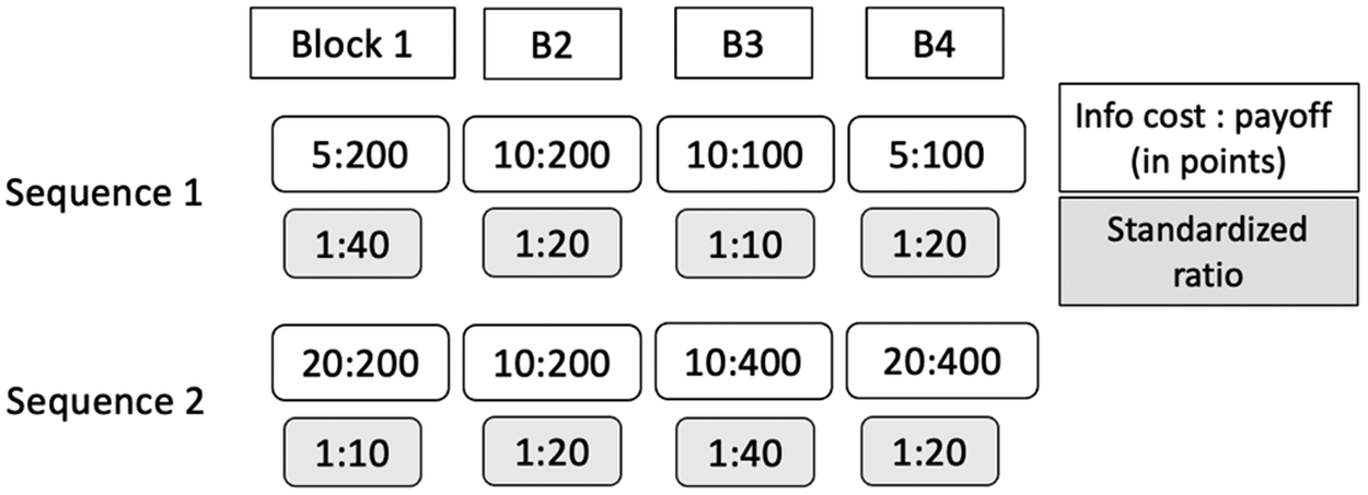
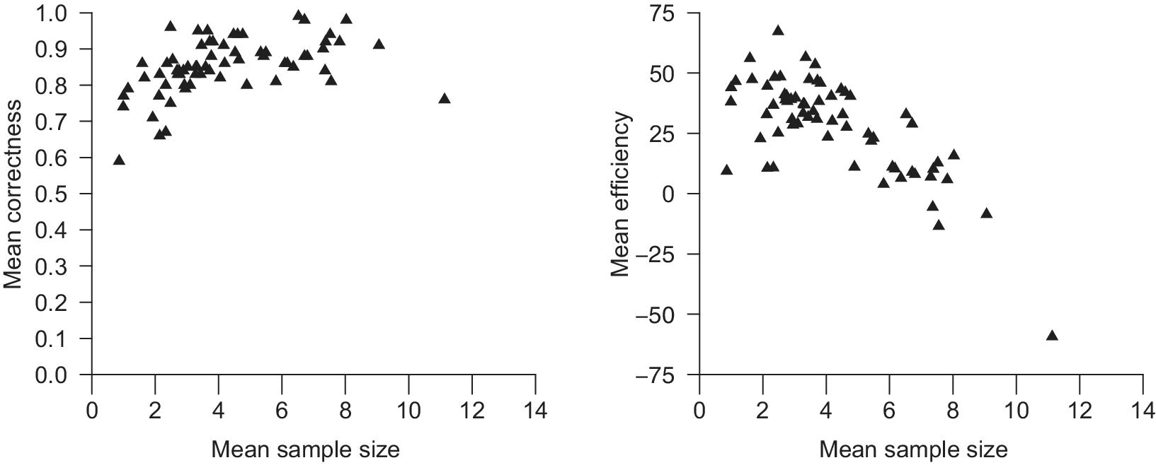
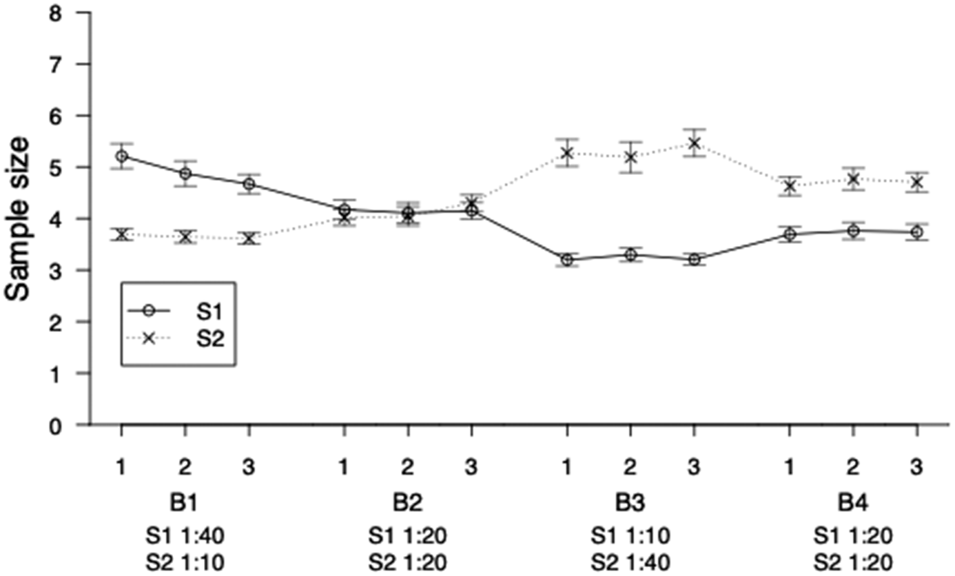
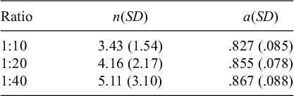
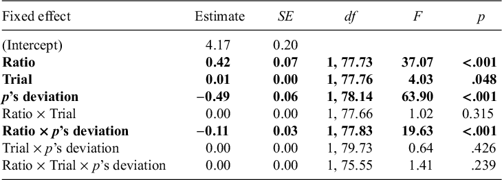
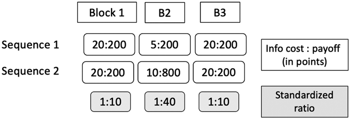
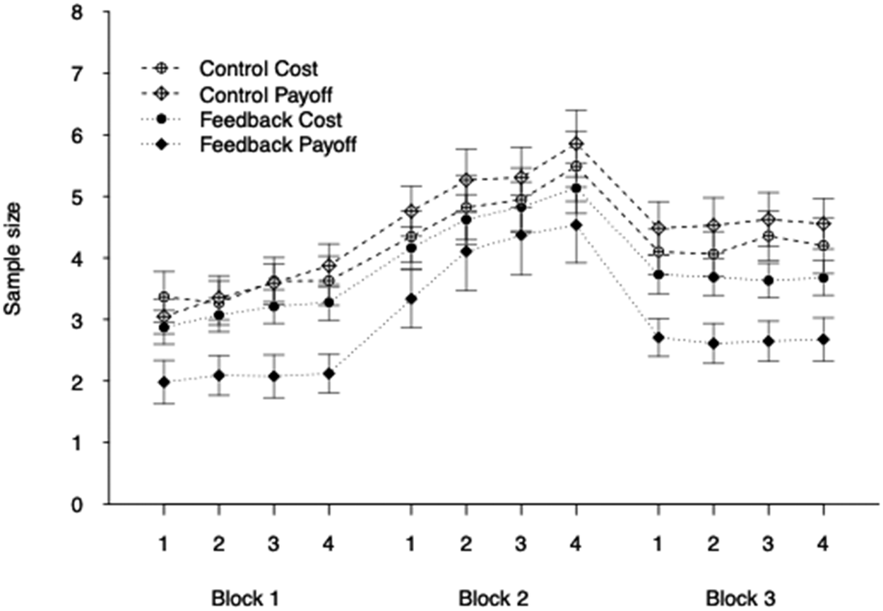
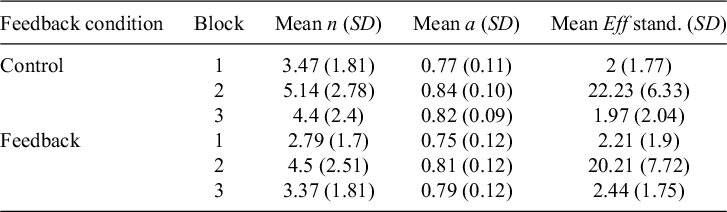
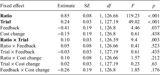
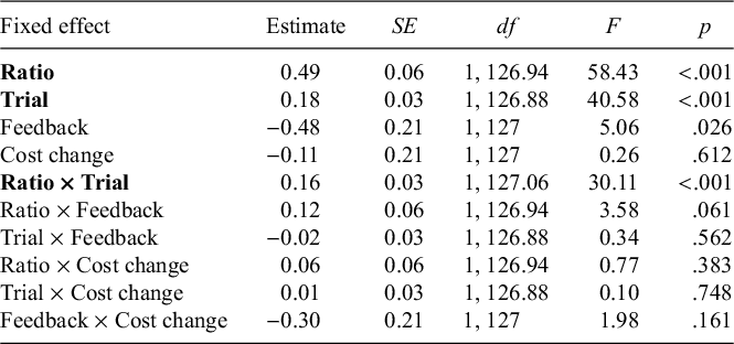
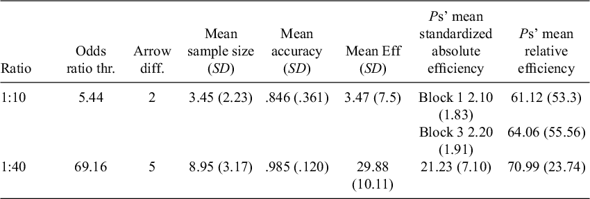
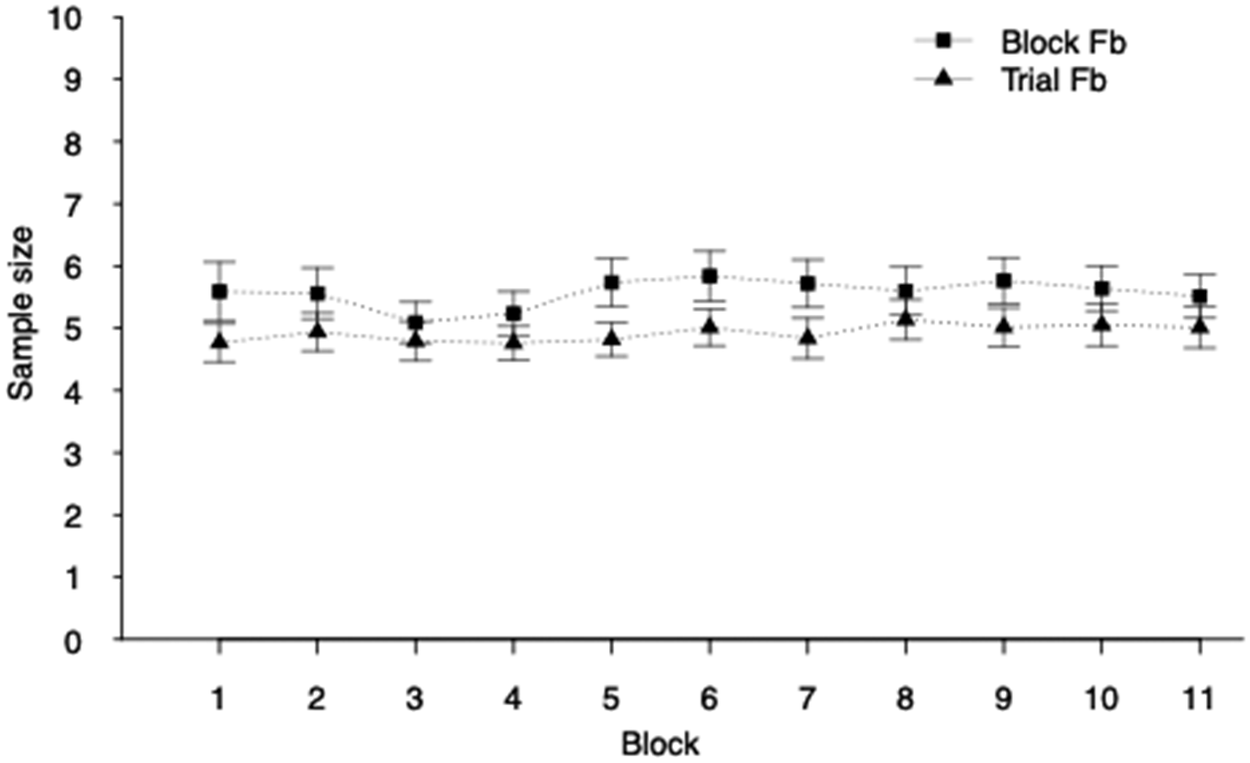
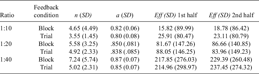
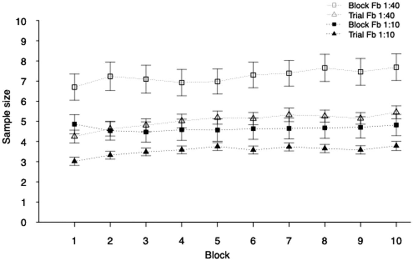
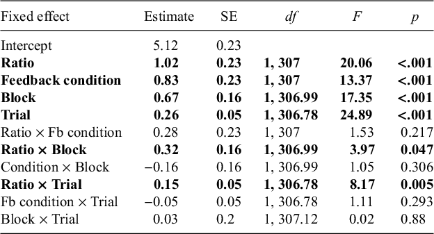
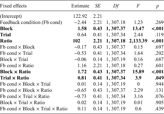
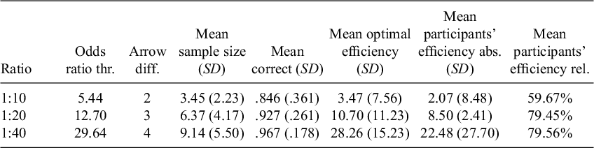
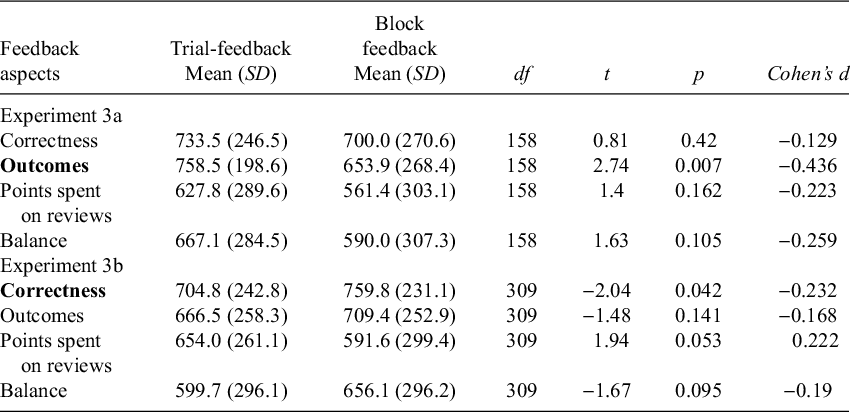
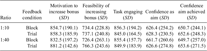


 Open access

