



1. Introduction
I did my Bachelors in chemical engineering from the University Department of Chemical Technology (UDCT, now ICT, Mumbai), a department known for its close ties to Indian industry – virtually all of the faculty engage in consultancy. A consequence was the strong emphasis of the curriculum on applications – each of our final-semester projects involved designing an entire chemical plant, no less! Within this ‘applied’ framework, however, there was the occasional course that allowed the few among us, with a more fundamental bent, a glimpse of the underlying physics. It was one such course, titled ‘Multiphase Reactors’, which inspired me to take up fluid mechanics as a lifelong pursuit. I still recall a particular statement made by the professor in class that started off as: ‘Kinetics is the same here in UDCT, Mumbai,
 $\ldots$
(pause)
 $\ldots$
and in Georgia, USA’. This was followed by a second (pregnant) pause, after which the professor went on to emphasise how, with reaction chemistry being fixed, reactor design was all about understanding the momentum, heat and mass transport processes involved; and that it is this understanding that allows for a scale-up of a process from the lab to industry. Coming from one of the highest-paid technical consultants in the country at the time, the choice of words, and the manner of delivery (to impressionable undergraduates), had a lasting impact.
It seems appropriate therefore to start out this perspectives with examples from chemical engineering, a discipline that abounds with instances of disperse multiphase systems, involving heat or mass transport between suspended drops/particles and a flowing ambient. Bubble column reactors, extensively used in the chemical, biochemical and petrochemical industries for a wide range of chemical processes, including oxidation, alkylation, fermentation (to name a few), due to their ease of operation and low maintenance costs, are a prominent example. The gaseous phase is introduced in the form of bubbles at the bottom, via a sparger (distributor). The gas bubbles then rise through the liquid column, during which time there is mass and heat transfer across their interfaces, often accompanied by a bulk chemical reaction in presence of suspended catalyst particles. The column dimensions are dictated, in part, by interfacial transport rates. The transport process involves diffusion from non-spherical bubbles undergoing shape oscillations and being subject to an inhomogeneous turbulent shearing flow that is particularly intense in wide columns operating in the so-called churn-turbulent regime (Joshi Reference Joshi2001; Kantarci, Borak & Ulgen Reference Kantarci, Borak and Ulgen2005). A second example is spray drying, a process used most often in the pharmaceutical industry and that is, in some sense, the inverse of the above-mentioned bubble column configuration – atomised liquid feed is sprayed down from the top into a heated gas stream (in a co- or counter-current configuration), with evaporation from the surfaces of the falling liquid droplets transforming them into a dry powder. Solvent extraction columns designed for selective transfer of a solute between immiscible liquids, one of which is dispersed in the other via suitable input of mechanical energy, constitute another example; an important application being the purification of uranyl nitrate, an intermediate step towards Uranium enrichment. Suspension polymerisation, used for manufacturing polystyrene beads, involves dispersing monomer drops in a low-viscosity medium, with each drop acting as a mini-reactor for an exothermic polymerisation reaction that gradually transforms it into a polymer particle. A key advantage over the analogous bulk process is efficient heat removal, due to a combination of the large interfacial area and mechanical agitation, allowing for tight control of the molecular weight distribution.
Important examples exist outside of chemical engineering. The spray combustion process inside internal combustion engines involves injection of fuel as a high-speed jet, from an atomiser into a turbulent air stream, with subsequent evaporation rates determining the engine combustion characteristics. Fuel drops arise from the original jet via a cascade of break-up events, triggered by a combination of surface tension and shear forces. The drops then move along complicated trajectories in the process of relaxing to the imposed flow, while evaporating into unsaturated air at high temperature and pressure, that slips past each drop in a turbulent fashion. Despite the complexity, much insight has been gained from single-drop models where, in the rapid-reaction limit, fuel vapour is transported away from the drop, while oxygen in air is transported inward, with the two reacting in a thin annular front; part of the heat of reaction diffuses inward, providing for the latent heat of fuel-drop vaporisation (Law Reference Law1982).
A few natural scenarios are worth mentioning. Marine phytoplankton, primarily unicellular autotrophs that form the base of the aquatic food web and contribute to carbon fixation, come in an astonishing range of shapes (Karp-Boss & Boss Reference Karp-Boss and Boss2016). They include swimming (dinoflagellates) (Karp-Boss et al. Reference Karp-Boss, Boss and Jumars1996) and non-swimming (diatoms) groups (Musielak et al. Reference Musielak, Karp-Boss, Jumars and Fauci2009), with uptake of nutrients (feeding) being a fundamental process in almost all cases. Convection due to swimming and/or an ambient flow (ocean currents, turbulence) plays a potentially crucial role in determining uptake rates of larger nutrient molecules. In the atmosphere, the initial stages of rain-cloud formation involve nucleation of drops on sub-micron aerosols that then grow by condensation in a weakly convecting supersaturated environment subject to turbulence-induced fluctuations in humidity (Shaw Reference Shaw2003). The initial condensational growth is an important element in determining the overall efficiency of rain-drop formation; the resulting drop-size distribution controls the cloud’s optical properties, which in turn influence the earth–atmosphere radiation budget. Gas transport from entrained bubble clouds, in the turbulent envinronment under breaking waves, is an important contributor to the overall gas exchange between the atmosphere and oceans (Deike Reference Deike2022).
The previous examples involve either or both heat and mass transport between suspended drops (particles) and a flowing environment. Due to the complexity of the overall transport scenario, one usually appeals to empirical wisdom, encapsulated in correlations for heat and mass transport rates, when designing an industrial equipment or modelling the natural phenomenon of interest. Now, transport driven by an imposed difference in temperature or concentration is a manifestation of a departure from equilibrium. In the absence of flow, it has a diffusive character, with the transport coefficients (the thermal or mass diffusivity) determined by the characteristics of the underlying molecular motion – the strength of the intermolecular forces that drive this motion and the time scale over which these forces de-correlate along molecular trajectories. Diffusivity is thus a material property. The momentum, mass and heat diffusivities are all
 $O(10^{-5}\,\text{m}^2\,\text{s}^{-1})$
for gases under normal conditions owing to the common underlying mechanism of transport (random streaming of molecules); in liquids, these diffusivities can differ from one another considerably, with mass diffusivities being at least three orders of magnitude smaller than for gases.
(a) Table of transport-rate correlations from Perry’s Chemical Engineers’ Handbook; reproduced with permission from Perry (Reference Perry1950). (b) The Sherwood number (
 ${\textit{Sh}}$
) versus Péclet number (
 ${\textit{Pe}}$
) plot demonstrating convectively enhanced scalar transport for a sphere in an ambient shearing flow (from: figure 5, p. 89, Nutrient fluxes to planktonic osmotrophs in the presence of fluid motion, by L. Karp-Boss, E. Boss and P. A. Jumars, Oceanography And Marine Biology ©1996 by Imprint. Reproduced by permission of Taylor & Francis Group). Equations (32) and (34) are small-
 ${\textit{Pe}}$
correlations, of the form
 $1+c {\textit{Pe}}^{{1}/{2}}$
, with
 $c = 0.36$
and
 $0.23$
. Equations (35) and (36) are large-
 ${\textit{Pe}}$
correlations, of the form
 $c {\textit{Pe}}^{{1}/{3}}$
, with
 $c=0.9$
and
 $0.63$
. Filled symbols denote computations for a sphere in a uniaxial extensional flow (Karp-Boss, Boss & Jumars Reference Karp-Boss, Boss and Jumars1996), and open circles denote experiments for heat transport from a sphere in a planar extension (Purcell Reference Purcell1978).

Figure 1. Long description
The table titled Mass-transfer correlations for flow past submerged objects contains three columns labeled Situation, Correlation, and Comments. It includes multiple rows detailing different scenarios such as a single sphere, a single sphere with creeping flow and forced convection, and single spheres with molecular diffusion and forced convection at low flow rates. Each row provides specific correlations and comments for empirical, semi-empirical, and theoretical use. The table also references various sources for further reading. The table has three columns and multiple rows, each row providing detailed information on different scenarios and their respective correlations.
Diffusive transport becomes increasingly inefficient on large scales. Thus, for the bubble column height to be of order a few metres, rather than a kilometre (!), one requires transport rates larger than that possible due to diffusion alone. For a given choice of materials (dictated by process requirements), this can be achieved via flow induced by mechanical stirring, an imposed pressure gradient or via buoyancy forces arising in a gravitational field. This brings in an additional bulk transport mechanism – convection. The general wisdom is that of convection enhancing transport rates – figure 1(a) shows the snapshot of a page from Perry’s handbook, a book we used extensively during our B.Tech, containing a table of empirical correlations, each of which has the non-dimensional transport rate (the Sherwood number, denoted as
 $N_{{\textit{Sh}}}$
therein; see § 2) increasing algebraically with the flow intensity (the Reynolds number, denoted
 $N_{{\textit{Re}}}$
). This increase may be interpreted as being due to a flow-induced reduction in the distance (the ‘film thickness’) over which the driving force (temperature or concentration difference) acts. With diffusion alone, this distance is of the order of the drop or particle size; it decreases with increase in the flow intensity, often reducing to a thin layer when convection is dominant. Herein, we attempt to understand the nature of the aforesaid film as a function of the geometry and strength of the imposed flow. The ultimate objective is to be able to use this understanding to reduce the element of empiricism in correlations such as those in figure 1(a). As will be seen, the parameter space governing convective transport is large and the manner of convective enhancement, the associated scaling laws, etc., can be very different in different regions of parameter space. Understanding the underlying mechanisms requires concepts drawn from transport phenomena as taught in chemical engineering curricula, the framework of matched asymptotic expansions, boundary layer theory, other perturbation techniques such as the method of multiple scales, and elements of non-equilibrium statistical mechanics and dynamical systems theory.
We proceed in a sequential fashion, beginning with the basic ideas and definitions in § 2. Next, in § 3, after laying out the requisite results pertaining to pure diffusion, we examine the weak convection limit in detail. Sections 4 and 5 examine the strong convection limit for particles and drops, respectively, with the one for drops bifurcated into §§ 5.1 and 5.2 that deal with the so-called exterior and interior problems. In this broad demarcation into portions that address the weak and strong convection limits, we follow the excellent textbooks of Gary Leal (Chapters 8 and 9 in Leal (Reference Leal1992); and Chapter 9 in Leal (Reference Leal2007)); transport rates over the intermediate parametric range can often be obtained via smooth interpolation between the above-mentioned limiting forms, as is seen from the convectively enhanced transport from a solid sphere immersed in two different shearing flows, shown in figure 1(a). The figure compares the Sherwood number from heat transfer experiments (Purcell Reference Purcell1978) with numerical computations (Karp-Boss et al. Reference Karp-Boss, Boss and Jumars1996), and theoretical correlations in the weak and strong convection limits. We will comment on aspects of this comparison, including the analytical forms of the correlations used, as we progressively develop our understanding. The dimensionless parameters pertaining to the scalar transport problems are given in table 1. A quick summary of the transport-rate predictions for small
 ${\textit{Pe}}$
is available from table 2. Detailed ensembles of large-
 ${\textit{Pe}}$
transport-rate predictions for the particle and drop cases, along with the places in the perspectives where they appear, are laid out in figures 9(b) and 15(b), respectively. Finally, in § 6, we outline important directions for future work.
Important dimensionless parameters for the scalar transport problem.
 $\varTheta$
and
 $\varTheta _0$
, in the
 ${\textit{Nu}}\,({\textit{Sh}})$
definition, satisfy (2.1) and (3.1), respectively; the associated boundary conditions being
 $\varTheta = \varTheta _0 = 1$
on
 $S_p$
, along with a far-field decay requirement.

Table 1. Long description
The table contains dimensionless parameters relevant to scalar transport problems. It includes the Peclet number, Nusselt number, Reynolds number, Capillary number, the ratio of drop and ambient fluid viscosities, the Strouhal number, and the spheroid aspect ratio. Each parameter is defined and associated formulas are provided. The table has two columns: the first column lists the parameters and the second column provides their definitions and formulas. The table helps in understanding the various dimensionless parameters involved in scalar transport problems and their mathematical representations.
2. Defining forced convection
Our concern here will be solving the convection-diffusion equation written in the following non-dimensional form:
 \begin{equation} \frac {\partial \varTheta }{\partial t} + \boldsymbol{u} \boldsymbol{\cdot }\boldsymbol{\nabla } \varTheta = \frac {1}{{\textit{Pe}}}{\nabla} ^2 \varTheta . \end{equation}
Here,
 $\varTheta (\boldsymbol{x},t)$
is an appropriately normalised temperature or concentration (scalar) field satisfying specific (Dirichlet or Neumann or mixed-type) conditions on all surfaces bounding the domain of interest. The flow within this domain is characterised by the velocity field
 $\boldsymbol{u}(\boldsymbol{x},t)$
. For instance, if one has transport of heat from a particle to an effectively unbounded colder fluid ambient, then
 $\varTheta = ({T - T_\infty })/({T_s - T_\infty })$
, where
 $T(\boldsymbol{x},t)$
is the temperature at a point
 $\boldsymbol{x}$
in the fluid, at time
 $t$
, and
 $T_s$
and
 $T_\infty$
denote the temperatures (assumed constant) at the particle surface and of the far-field ambient, respectively; an analogous expression in terms of concentrations applies for the mass transport scenario. The absence of source terms in (2.1) implies
 $\varTheta$
is bounded between
 $0$
and
 $1$
, with these extremal values only being attained at boundaries – the particle surface and, for the case of an unbounded domain, the surface at infinity. (These bounds rigorously hold for
 ${\textit{Pe}} = 0$
owing to the maximum principle associated with Laplace’s equation; convection, for finite
 ${\textit{Pe}}$
, only leads to a flow-induced rearrangement of the scalar field. In the fluid mechanical context, the same principle applied to potential flow, for instance, implies that the maximum speed can occur only on bounding surfaces.) The objective is to calculate the scalar transport rate from the particle or drop which is typically scaled by the transport rate due to diffusion alone. This non-dimensional ratio is termed the Nusselt number (
 ${\textit{Nu}}$
) for heat transport and the Sherwood number (
 $Sh$
) for mass transport.
The focus here is on the classical forced convection scenario where
 $\boldsymbol{u}(\boldsymbol{x},t)$
in (2.1) is assumed incompressible and is specified a priori, having been obtained independently from solving the equations of motion. As evident from (2.1), the key dimensionless parameter is the Péclet number,
 ${\textit{Pe}}= Ua/D$
, which compares the magnitudes of the convection (
 $\boldsymbol{u} \boldsymbol{\cdot }\boldsymbol{\nabla } \varTheta$
) and diffusion (
 ${\nabla} ^2 \varTheta$
) terms in (2.1); here,
 $U$
is an appropriate velocity scale,
 $a$
the characteristic particle (drop) size and
 $D$
the thermal or mass diffusivity. Here,
 ${\textit{Pe}}$
is the primary determinant of the nature of the scalar field, and thence, the transport rate. Indeed, the solution of a forced convection problem may be characterised by
 ${\textit{Nu}}$
or
 ${\textit{Sh}}$
expressed as a function of
 ${\textit{Pe}}$
, as in figure 1(b). Importantly, this functional dependence, for arbitrary
 ${\textit{Pe}}$
, can often be obtained by simple interpolation between asymptotic forms known in the diffusion-dominant (
 ${\textit{Pe}} \ll 1$
) and convection-dominant (
 ${\textit{Pe}} \gg 1$
) limits. Such interpolated forms are the basis of empirical correlations used in practice – see figure 1(a). For arbitrary
 ${\textit{Pe}}$
, the complicated spatial dependence of
 $\boldsymbol{u}$
necessitates a numerical approach for solving (2.1), and hence, as also evident from the previous organisational paragraph, our emphasis is on the aforementioned asymptotic forms.
Before delving deeper into the nature of the solutions of (2.1), it is worth laying out, in some detail, the assumptions that have gone into writing down (2.1).
-
(i) Although we mention
 $\boldsymbol{u}(\boldsymbol{x},t)$
in (2.1) as being determined independently of
$\varTheta$
, strictly speaking, this is impossible in the presence of a gravitational field. Buoyancy-induced convection invariably arises due to density variations associated with temperature (concentration) differences. We assume any such free-convection-induced contribution to be negligibly small compared with that due to forced convection, pointing to the smallness of an appropriately defined Grashof number.
-
(ii) Constancy of all other physical properties (specific heat, thermal conductivity, mass diffusivity, viscosity, etc.) is assumed, thereby imposing a restriction on the magnitude of the difference between the surface and ambient temperatures (concentrations) that drives transport. Even in scenarios where such differences are large, use of constant physical properties, defined at a value intermediate between the boundary values (this being termed the 1/2 or 1/3 rule in the spray-combustion literature, depending on the specific combination of fuel-drop and ambient-air temperatures used; see Law (Reference Law1982)), leads to reliable predictions.
-
(iii) Coupling of heat and mass transport problems due to phase changes (and the latent heat or heat of solution involved), as can occur in both natural (growth of cloud condensation nuclei) and man-made (evaporation of fuel drops following spray injection) scenarios, is neglected.
-
(iv) Even in the absence of phase change, the assumed equivalence of heat and mass transport scenarios, implicit in (2.1), needs clarification since, in the latter case, the presence of two or more components leads to a more complicated picture. Considering the case of a fuel drop evaporating into ambient air, the no-flux boundary condition on the drop surface, reflecting the insolubility of air (in fuel), necessitates a bulk flow that balances the inward diffusive flux of air at the surface, that then contributes to the outward convection of fuel vapour. This contribution, the so-called Stefan flow, is always present in a multi-component situation, independent of any coupling induced by the latent heat of vaporisation (Sazhin Reference Sazhin2006; Erbil Reference Erbil2012), but is neglected here; an assumption valid for sufficiently small mass transport (evaporation) rates. Much higher transport rates lead to other subtleties such as a Knudsen layer in the immediate neighbourhood of small drops, interfacial resistance to molecular transport leading to deviations from saturation conditions at the interface, etc., that have been discussed elsewhere (Sazhin Reference Sazhin2006) and will not be considered here.
-
(v) Occurrence of reactions in either the bulk or at the interface, as is common for processes in the chemical industry, is neglected.
-
(vi) Viscous and radiative heating effects, which when present would lead to source terms in (2.1), are neglected.


Neglect of free convection effects, together with the assumed constancy of physical properties, leads to (2.1) being a linear partial differential equation. Linearity implies that there can be no analogue of the boundary layer separation, that occurs in the momentum-transport problem at large Reynolds numbers (
 ${\textit{Re}} = Ua/\nu$
,
 $\nu = \mu /\rho$
being the kinematic viscosity of the fluid;
 $\mu$
and
 $\rho$
are the viscosity and density of the ambient fluid), for large
 ${\textit{Pe}}$
. Thus, even for flow past bluff bodies, the thermal or concentration wake remains asymptotically thin for sufficiently large
 ${\textit{Pe}}$
and the leading order transport rate may be calculated within the framework of an (attached) boundary layer formulation. It must be kept in mind, however, that separation of the momentum boundary layer and the resulting recirculating eddies still determine the the scalar wake location and the ‘scalar ambient’ seen by the drop or particle. Thereby,
 ${\textit{Re}}$
can indirectly influence the magnitude of the transport rate, although not its
 ${\textit{Pe}}$
-scaling (when the eddies are steady). An instance of transport in the presence of recirculating eddies, induced by a surface velocity reversal, will be seen in the context of nutrient uptake by microswimmers, in § 5.1.4.
Although
 ${\textit{Pe}}$
plays a key role in determining
 ${\textit{Nu}}$
(from now onward,
 ${\textit{Nu}}$
is taken to denote the non-dimensional scalar transport rate, of either heat or mass, in diffusion units), other dimensionless parameters enter (2.1) via
 $\boldsymbol{u}$
, among which the role of
 $Re$
has been previously highlighted. One may write the general functional form:
 \begin{equation}{\textit{Nu}}= {\mathcal F}_p({\textit{Pe}},{\textit{Re}},\{S\},\{P\}) \end{equation}
for a solid particle, and
 \begin{equation}{\textit{Nu}}= {\mathcal F}_d({\textit{Pe}},{\textit{Re}},\lambda ,Ca,\{P\}) \end{equation}
for a drop in an ambient flow. In (2.2),
 $\{ S\}$
denotes the set of particle shape parameters and is an empty set for a sphere that is completely characterised by its radius
 $a$
(already contained in
 ${\textit{Pe}}$
);
 $\{S \}$
would include the aspect ratio(s) for particles of spheroidal and ellipsoidal geometries. For a drop, interfacial tension forces ensure sphericity in the absence of flow. In (2.3), the capillary number,
 ${\textit{Ca}} = \mu U/\varGamma$
(
 $\varGamma$
being the interfacial tension coefficient) is the ratio of viscous (
 $\mu U/a$
) to interfacial (
 $\varGamma /a$
) stresses, and along with
 $Re$
, determines drop deformation due to the ambient flow;
 ${\textit{Ca}}$
may be regarded as a flow-dependent shape parameter. In (2.3),
 $\lambda$
is the ratio of the drop (
 $\lambda \mu$
) and ambient (
 $\mu$
) fluid viscosities. For a drop, even in presence of convection, the dominant resistance to transport may occur either within (the interior problem) or in the ambient (the exterior problem). In the general case where the transport resistances in the two phases are comparable, the so-called conjugate problem, the ratio of the drop and ambient thermal conductivities (or mass diffusivities) also plays a role via the interfacial conditions. Herein, we only examine cases where either of the aforementioned resistances is dominant, a scenario often facilitated by a fast reaction occurring in one of the phases.
In (2.2) and (2.3),
 $\{ P \}$
denotes the set of flow-type parameters that define the geometry of the ambient flow. Note the distinction between
 $\{ P \}$
and
 ${\textit{Re}}$
– the latter determines the nature of the actual flow around the particle or drop for a given ambient flow. For instance, recirculating eddies arise for a translating particle beyond a threshold
 ${\textit{Re}}$
, owing to separation of the actual flow as it decelerates along the particle surface. In contrast, the nature of the ambient flow is governed by dynamics on a scale (say,
 $L_m$
) much larger than the particle (drop) size. The implicit assumption is therefore that of particles or drops being sufficiently small compared with the characteristic scale(s) of the ambient flow, that is,
 $a/L_m \ll 1$
. This allows for a Taylor expansion of the ambient flow about the particle (drop) location, in a reference frame moving along with it. Successive terms in this expansion are smaller by
 $O(a/L_m)$
, with the leading order term being:
-
(i) a uniform flow for particles or drops that translate relative to the ambient;
-
(ii) a linear shearing flow for particles or drops that do not.
The translational slip in case (i) is usually due to a density difference between particle (drop) and the ambient. Denoting the slip velocity as
 $U_t$
, the choice of an ambient uniform versus linear flow is determined by the ratio
 $U_t/(\dot {\gamma }a)$
,
 $\dot {\gamma }$
being the shear rate, a characteristic scale for the magnitude of the (constant) velocity gradient tensor that dictates the geometry of the linear flow;
 $\dot {\gamma }a$
is then the velocity scale for the shear flow around the particle (drop). Herein, we mainly examine neutrally buoyant particles (drops), corresponding to
 $U_t/(\dot {\gamma }a) \ll 1$
. In our emphasis on ambient linear flows, we depart from most earlier reviews which focus on aspects of slip-induced transport enhancement (Michaelides Reference Michaelides2003; Sazhin Reference Sazhin2014; Balachandar & Michaelides Reference Balachandar and Michaelides2021).
With
 $\dot {\gamma }a$
as the characteristic velocity scale for an ambient linear flow, the dimensionless parameters in the
 ${\textit{Nu}}$
-functionals, in (2.2) and (2.3), are given by
 ${\textit{Pe}} = \dot {\gamma }a^2/D$
,
 ${\textit{Re}} = \dot {\gamma }a^2/\nu$
and
 ${\textit{Ca}} = \mu \dot {\gamma }a/\varGamma$
;
 ${\textit{Re}}$
in particular may be termed the micro-scale Reynolds number. The previous small
 $a/L_m$
assumption implies a restriction on the magnitudes of these parameters. Thus, in what follows, we will assume
 $Re$
and
 ${\textit{Ca}}$
to be zero, except in cases where even weak effects of inertia or deformation lead to a qualitatively different transport scenario. As mentioned in § 1, the smallness of the mass diffusivity (
 $D$
), renders
 ${\textit{Pe}}$
, for mass transport in liquids, large even when
 ${\textit{Re}}$
is not. Thus, we examine both small-
 ${\textit{Pe}}$
(§ 3) and large-
 ${\textit{Pe}}$
(§§ 4 and 5) transport scenarios.
Linear shearing flows have a non-trivial geometry (Chong, Perry & Cantwell Reference Chong, Perry and Cantwell1990). Since the ambient flow determines the topology of the streamlines near the particle or drop surface, and the latter control transport across a thin boundary layer at large
 ${\textit{Pe}}$
, ambient flow geometry can have a profound effect on transport rates in this limit. As will be seen in §§ 4 and 5, therefore,
 $\{ P \}$
in (2.2) and (2.3) plays an important role in determining
 ${\textit{Nu}}$
. From the viewpoint of classifying different transport scenarios, it becomes convenient to organise linear flows in an appropriate parameter space. In § 3.1, incompressible linear flows will be seen to exist in a four-dimensional (4-D) space, implying that
 $\{ P\}$
comprises four scalar geometrical parameters. Such an organisation is useful even when the ambient flow is unsteady or turbulent. Sub-Kolmogorov particles (drops) see turbulence as a fluctuating linear flow and the statistical sampling of linear flow topologies is known to be non-uniform (Meneveau Reference Meneveau2011), being determined by an appropriate macro-scale (the Taylor microscale!) Reynolds number. This again highlights the distinction, implicit in (2.2) and (2.3), between the macro-scale flow dynamics (which enters via
 $\{ P\}$
) and micro-scale flow dynamics (which enters via
 $Re$
), both of which influence transport rates.
Finally, it is worth adding that (2.2) and (2.3), with
 ${\textit{Pe}}$
,
 $Re$
and
 ${\textit{Ca}}$
defined in terms of
 $\dot {\gamma }$
, assume a steady ambient linear flow, this being tantamount to there being a unique flow time scale of
 $O(\dot {\gamma }^{-1}$
). Although the discussion here is largely restricted to steady ambient flows, we will, on occasion, comment on the role of unsteadiness. When the ambient flow has a time-periodic character, the ratio of the frequency of oscillation (
 $\omega$
) to the shear rate, the Strouhal number (
 $Sl = \omega /\dot {\gamma }$
), enters as an additional parameter in (2.2) and (2.3); for stochastic ambient flows, including turbulence,
 $\omega$
is to be replaced by an appropriate (inverse) correlation time.
3. Weak convection limit
In terms of the nominal scale
 $a$
used in § 2, weak convection corresponds to
 ${\textit{Pe}} = \dot {\gamma }a^2/D$
being small. However, when defining
 ${\textit{Pe}}$
for non-spherical particles, one has multiple length scales to choose from, and for extreme geometries, the
 ${\textit{Pe}}$
values obtained from the different choices are asymptotically separated in magnitude. In § 3.1, we consider the case where
 ${\textit{Pe}}$
based on even the largest particle dimension is small. In this limit, convective effects only lead to a small correction to the leading order diffusive transport rate, although the associated scaling is important – it pertains to the small-
 ${\textit{Pe}}$
correlations in figure 1(b) and is indicative of the singular nature of weak convection; the latter nature manifests as different scalings for ambient uniform vis-à-vis linear flows. Calculation of this correction helps illustrate the utility of a Fourier-space approach, as opposed to the classical matched asymptotic expansions framework. In § 3.2, we show that, for sufficiently slender particles, the logarithmic smallness of the disturbance velocity field, on scales of the order of the particle length, allows one to calculate the transport rate using the Fourier-space formulation of § 3.1, even when
 ${\textit{Pe}}$
based on the largest dimension (particle length) is of order unity, provided
 ${\textit{Pe}}$
based on the cross-sectional dimension remains small. Section 3.3 examines the two-dimensional (2-D) scenario of transport from a circular cylinder. The largest dimension (cylinder length) and the associated
 ${\textit{Pe}}$
have now diverged to infinity, with the leading order transport rate exhibiting a logarithmic dependence on the (small) Péclet number based on the radius, a signature of the Stokes paradox.
Before considering convective effects in § 3.1, we examine the baselined diffusive scenario. With
 ${\textit{Pe}} = 0$
and assuming a quasi-steady scenario in (2.1), one obtains Laplace’s equation:
 \begin{equation} {\nabla} ^2 \varTheta = 0 \end{equation}
for the scalar field. Solving (3.1) with the appropriate boundary conditions yields the diffusive transport rate (
 $Q_0$
), which then serves as the normalisation when defining
 ${\textit{Nu}}$
. Here,
 $Q_0$
is the ‘diffusion unit’ in which one measures transport enhancement – see table 1.
To understand the dependence of
 $Q_0$
on particle shape, we start with the simplest case: that of an isothermal hot sphere in a stagnant medium, whence (2.1) takes the form
 \begin{equation} \frac {1}{r^2}\frac {\partial }{\partial r} \left ( r^2 \frac {\partial \varTheta }{\partial r} \right ) = 0, \end{equation}
with
 $\varTheta = 1$
at
 $r = 1$
and
 $\varTheta \rightarrow 0$
for
 $r \rightarrow \infty$
. The solution is
 $\varTheta = {1}/{r}$
, the fundamental solution (Green’s function) of Laplace’s equation in three dimensions – spherical symmetry ensures that, as far as the scalar field in the exterior is concerned, a sphere is equivalent to a point source at its centre. The diffusive transport rate may be evaluated as the integral of the normal component of the scalar flux (given by Fourier’s law as
 $\boldsymbol{q} = -k \boldsymbol{\nabla } T$
,
 $k$
being the thermal conductivity, for heat transport) over the sphere surface. This gives
 \begin{align} Q_0 = &-k \displaystyle \int \boldsymbol{n} \boldsymbol{\cdot }\boldsymbol{\nabla } T \vert _{r=a} \,\text{d}S = -k a(T_s - T_\infty ) \displaystyle \int \boldsymbol{n} \boldsymbol{\cdot }\boldsymbol{\nabla } \varTheta \vert _{r=1}\, \text{d}\varOmega , \end{align}
where the second integral is over the unit sphere,
 $\boldsymbol{n}$
being the unit outer normal and
 $\text{d}\varOmega$
being a differential solid angle element. Using
 $\varTheta = {1}/{r}$
gives
 $\boldsymbol{n} \boldsymbol{\cdot }\boldsymbol{\nabla } \varTheta \vert _{r=1} = ({\partial \varTheta }/{\partial r}) = -1$
and the integral reduces to the area of a unit sphere yielding
 \begin{equation} Q_0 = 4\pi a k (T_s - T_\infty ). \end{equation}
The diffusive transport rate scales linearly with
 $a$
, since the quadratic scaling of the surface area is compensated by the decrease of the scalar gradient as
 $a^{-1}$
; an
 $a^2$
-scaling can only arise in a near-vacuum ambient where the transport would have a ballistic character. Knowing
 $Q_0$
and using the equivalence of the sphere to a point source, one may write the governing equation for the scalar field in the form
 \begin{equation} {\nabla} ^2 \varTheta = - 4\pi \delta (\boldsymbol{x}), \end{equation}
where the delta-function forcing accounts for the surface boundary condition. In (3.5),
 $\varTheta$
is defined over the entire domain including the sphere interior which, as will be seen, is convenient in accounting for weak convection effects within a Fourier-space formulation.
Next, to illustrate differences arising due to departure from spherical symmetry, we consider an isothermal spheroid in a stagnant fluid ambient, The surface boundary condition takes the form
 $\varTheta = 1$
at
 $\xi = \xi _0$
in spheroidal coordinates,
 $\xi$
being the analogue of the radial distance in spherical coordinates, with
 $\xi _0$
denoting the spheroid surface and being related to the spheroid aspect ratio
 $\kappa$
;
 $1 \leqslant \xi , \xi _0 \lt \infty$
, with
 $\xi _0 = {\kappa }/{(\kappa ^2-1)^{{1}/{2}}}$
for prolate spheroids (
 $\kappa \gt 1$
) and
 $\xi _0 = {1}/{(1-\kappa ^2)^{{1}/{2}}}$
for oblate spheroids (
 $\kappa \lt 1)$
. For the prolate case, Laplace’s equation takes the form
 \begin{equation} \frac {1}{(\xi ^2-\eta ^2)} \frac {\partial }{\partial \xi } \left [ (\xi ^2-1) \frac {\partial \varTheta }{\partial \xi } \right ] = 0, \end{equation}
where, motivated by the boundary condition, we have omitted dependence of
 $\varTheta$
on the other two coordinates (prolate spheroidal coordinates
 $(\xi ,\eta ,\phi )$
are related to the Cartesian ones as
 $x_1 + \mathrm{i}x_2= {d}\bar {\xi }(1-\eta ^2)^{{1}/{2}}\textit{e}^{\mathrm{i}\phi }$
,
 $x_3 = {d}\xi \eta$
,
 $x_3$
-axis being the polar axis;
 $\xi \leftrightarrow \mathrm{i}\bar {\xi }$
,
 $d \leftrightarrow -\mathrm{i}d$
yield the oblate spheroidal coordinates, with
 $\bar {\xi } = (\xi ^2-1)^{{1}/{2}}$
. The constant-
 $\xi$
surfaces are confocal prolate (oblate) spheroids; the minimal prolate surface is the focal segment of length
 $2d$
, while the minimal oblate one is a focal disk with this diameter. Constant-
 $\eta$
surfaces are two-sheeted (single-sheeted) hyperboloids, and constant-
 $\phi$
surfaces are planes containing the axis of symmetry. The metric factors for the system are:
 $h_\xi = {{d}(\xi ^2 - \eta ^2)^{1/2}}/{(\xi ^2-1)^{1/2}}$
,
 $h_\eta = {{d}(\xi ^2 - \eta ^2)^{1/2}}/{(1-\eta ^2)^{1/2}}$
and
 $h_\phi = { d}(\xi ^2-1)^{1/2} (1-\eta ^2)^{1/2}$
(Kushch Reference Kushch2013; Dabade, Marath & Subramanian Reference Dabade, Marath and Subramanian2015)). The solution of (3.6) satisfying the far-field decay condition is
 \begin{equation} \varTheta = \left [ \ln \frac {\xi _0 + 1}{\xi _0-1} \right ]^{-1} \ln \frac {\xi + 1}{\xi -1}, \end{equation}
with the diffusive transport rate given by
 \begin{align} Q_0 &= -k(T_s -T_\infty ) \displaystyle \int \boldsymbol{1}_\xi \boldsymbol{\cdot }\boldsymbol{\nabla } \varTheta \vert _{\xi = \xi _0}\,\text{d}S, \end{align}
 \begin{align} &= - k(T_s - T_\infty ) \displaystyle \int _{-1}^1 \displaystyle \int _0^{2\pi } \frac {1}{h_\xi }\frac {\partial \varTheta }{\partial \xi } \vert _{\xi = \xi _0} (h_\eta \,\text{d}\eta ) (h_\phi \,\text{d}\phi ). \end{align}
Using the expressions for the metric factors
 $(h_\xi ,h_\eta ,h_\phi )$
gives
 \begin{equation} Q_0 = \frac {8\pi kd (T_s-T_\infty )}{\ln \left(\dfrac{\xi _0 + 1}{\xi _0-1} \right)} \end{equation}
for a prolate spheroid. The prolate–oblate transformation leads to
 \begin{equation} Q_0 = \frac {4\pi kd(T_s - T_\infty )}{\tan ^{-1} \bar {\xi }_0^{-1}} \end{equation}
for an oblate spheroid. In the limit
 $\xi _0 \rightarrow 1$
, corresponding to a slender fibre of length
 $L = 2{d}\xi _0 \approx 2d$
,
 $Q_0 = 2\pi k L(T_s-T_\infty )/\ln (2\kappa )$
, a result that will be used in § 3.2. In the same limit, (3.11) gives
 $Q_0 = 8kd(T_s-T_\infty )$
, corresponding to a disk with radius
 $d$
. These limiting expressions show that it is the largest geometrical dimension (fibre length or disk radius) that governs diffusive transport even from spheroids of extreme aspect ratios; for the fibre, there is only a weak logarithmic dependence on the diameter.
Unlike the sphere, the diffusive flux at the spheroid surface is non-uniform, increasing towards the ends which are regions of higher curvature. This increase is due to the clustering of flux lines and is typical of Laplace solutions – the latter are smooth in the domain interior, but singular at boundary points that are geometrical singularities. It may be shown, using (3.7) and its oblate analogue, that the normal flux components are proportional to
 ${2}/{(d(\xi _0^2 -1)^{{1}/{2}}(\xi _0^2 -\eta ^2)^{{1}/{2}}\ln [({\xi _0+1})/({\xi _0-1})]})$
and
 ${1}/{(d(\bar {\xi }_0^2 +1)^{{1}/{2}}(\bar {\xi }_0^2 +\eta ^2)^{{1}/{2}}\tan ^{-1}\bar {\xi }_0^{-1}})$
for prolate and oblate spheroids, respectively. The flux at the ends (
 $\eta = 1)$
of a slender prolate spheroid is
 $O[1/(d(\xi _0-1))] \approx O(\kappa ^2/L)$
, while that at the equator (
 $\eta = 0$
) of a thin oblate spheroid is
 $O[1/({d}\xi _0)] \approx O(1/(\kappa ^2 d))$
– both estimates show the flux scaling inversely as the local radius of curvature, diverging as the spheroid end sharpens to a point (edge). Indeed, regarding half of an oblate spheroid as an approximation of a sessile drop on a flat substrate, the increased diffusive flux close to the pinned edge is what drives the coffee-ring effect – the phenomenon named after the ring-like deposit left along the perimeter of a coffee spill after evaporation (Deegan et al. Reference Deegan, Bakajin, Dupont, Huber, Nagel and Witten1997). The nearly divergent local fluxes only occur over an asymptotically small neighbourhood of the ends, and the overall transport, as mentioned previously, still scales with the largest geometrical dimension.
Similar to (3.5), the spheroid surface boundary condition may be incorporated as a singular forcing. Unlike a sphere, a prolate spheroid is equivalent to a uniform distribution of sources along the focal segment, and (3.5) generalises to
 \begin{equation} {\nabla} ^2 \varTheta = - \frac {4\pi }{\ln \left(\dfrac{\xi _0 + 1}{\xi _0-1}\right)}\displaystyle \int _{-(2\xi _0)^{-1}}^{(2\xi _0)^{-1}} \delta (\boldsymbol{x} - s \boldsymbol{p})\,\text{d}s, \end{equation}
with
 $L$
used for non-dimensionalisation;
 $\boldsymbol{p}$
here denotes the unit vector along the spheroid orientation. For
 $r \gg \xi _0^{-1}$
, the right-hand side reduces to
 $-\bar {Q}_0\delta ({\boldsymbol{x}})$
, corresponding again to a point source, leading to the far-field form,
 $\bar {Q}_0/(4\pi r)$
, with
 $\bar {Q}_0 =4\pi (\xi _0\ln (({\xi _0 + 1})/({\xi _0-1})))^{-1}$
being the non-dimensional version of (3.10). Interpreted in dimensional terms,
 $Q_0/(4\pi r)$
is, in fact, the general far-field form of the diffusion solution since an arbitrarily shaped particle acts as a point source at sufficiently large distances.
We have thus far only examined the steady diffusion-dominant limit. The unsteady problem can be solved in closed form for a sphere and we discuss this solution in the context of the interior problem in § 5.2. Herein, we only note that the approach to steady state is monotonic and occurs on a time scale of
 $O(a^2/D)$
for spherical particles, with
 $a$
replaced by the largest geometrical dimension for non-spherical ones.
3.1. Spherical particles, drops and non-spherical particles with order unity aspect ratios
We now examine the first correction to the diffusive transport rate due to convective effects. This is a classic singular perturbation problem, and a better illustration of what has come to be known as Whitehead’s paradox in the momentum-transport scenario – the failure to obtain the inertial correction to the Stokes drag on a translating sphere using a regular perturbation (in
 $Re$
) approach, owing to the far-field decay requirement not being satisfied at
 $O(Re)$
– see Chapter 8 of Leal (Reference Leal1992). To illustrate this paradox in the context of scalar transport, we begin with an ambient uniform flow (with
 ${\textit{Pe}} = Ua/D$
). As already mentioned, the convective contribution to the scalar transport rate, for the order unity aspect ratios examined in this subsection, is small for small
 ${\textit{Pe}}$
. But, even weak convection profoundly alters the structure of the scalar field at large distances from the particle (drop), giving rise to a wake whose geometry depends crucially on the ambient flow-type, and is not necessarily limited by the smallness of
 ${\textit{Pe}}$
. Thus, a study of weak convective effects is important from the conceptual point of view.
3.1.1. First convective correction: uniform flow
To see why a straightforward expansion of the form
 $\varTheta = \varTheta _0 + {\textit{Pe}}\,\varTheta _1 + \cdots$
,
 $\varTheta _0$
being the diffusion solution previously obtained, does not work, we examine the relative importance of the convection and diffusion terms in (2.1). For small
 ${\textit{Pe}}$
, convection only becomes important at distances from the particle much larger than its largest dimension. At such distances, the particle appears as a point source, so one may use
 $\varTheta _0 \approx {1}/{r}$
for obtaining estimates. Doing so, one finds
 ${\nabla} ^2 \varTheta \sim {1}/{r^3}$
and
 $\boldsymbol{u} \boldsymbol{\cdot }\boldsymbol{\nabla } \varTheta \sim \hat {\boldsymbol{U}} \boldsymbol{\cdot }\boldsymbol{\nabla } ({1}/{r}) \sim {1}/{r^2}$
, where we have used
 $\boldsymbol{u} \approx \hat {\boldsymbol{U}}$
,
 $\hat {\boldsymbol{U}}$
being the unit vector along the ambient flow. The ratio of convection to diffusion terms is given by
 ${{\textit{Pe}}(\boldsymbol{u} \boldsymbol{\cdot }\boldsymbol{\nabla } \varTheta )}/({{\nabla} ^2 \varTheta }) \sim ({{\textit{Pe}}/r^2})/({1/r^3}) = {\textit{Pe}}\,r$
, implying that convection becomes important when
 $r \sim O({\textit{Pe}}^{-1})$
or, in dimensional terms, at distances of
 $O(D/U)$
, this being the convective screening length. This contradicts the assumption implicit in the small-
 ${\textit{Pe}}$
expansion given previously, of convection being a perturbative influence everywhere in the domain. The implication is that the diffusion solution is a valid leading order approximation and convection a perturbative effect, only for
 $r \ll O({\textit{Pe}}^{-1})$
, corresponding to the so-called inner region. However, one has to account for convection at leading order for
 $r \gtrsim O({\textit{Pe}}^{-1})$
, the so-called outer region. The characteristic scale in the outer region is not
 $a$
(the particle or drop is a point source) but
 $D/U$
. Not accounting for this change in scale and using the above-mentioned regular expansion would, at
 $O({\textit{Pe}})$
, lead to
 $\varTheta _1$
satisfying
 \begin{equation} {\nabla} ^2 \varTheta _1 = \boldsymbol{u} \boldsymbol{\cdot }\boldsymbol{\nabla } \varTheta _0. \end{equation}
Here,
 $\varTheta _1 = 0$
at the particle (drop) surface and must also decay in the far field. As noted already,
 ${\boldsymbol{u}} \boldsymbol{\cdot }\boldsymbol{\nabla } \varTheta _0 \sim O(1/r^2)$
for
 $r \gg 1$
, and therefore,
 ${\nabla} ^2 \varTheta _1 \sim O(1/r^2)$
, implying that
 $\varTheta _1$
asymptotes to an
 $r$
-independent limiting form at large distances. The resulting conflict with the far-field decay requirement is Whitehead’s paradox.
The paradox is resolved in a matched asymptotic expansions approach, since the expansion
 $\varTheta = \varTheta _0 + Pe\,\varTheta _1 + \cdots$
is now restricted to the inner region and the far-field decay requirement replaced by the requirement of matching with the near-field limiting form of an outer-region expansion (described later), valid at large distances. The interpretation as an inner-region expansion does not, however, mean that the expansion proceeds in powers of
 ${\textit{Pe}}$
, as for a regular perturbation problem – the previous matching requirement leads to logarithmic corrections and the next term (
 $\varTheta _2$
) in the expansion is, in fact,
 $O({\textit{Pe}}^2\ln {\textit{Pe}})$
; see § 3.1.3. Now, for all fore–aft symmetric particles,
 $\varTheta _0$
is an even function of
 $\boldsymbol{x}$
, satisfying
 $\varTheta _0(\boldsymbol{x}) = \varTheta _0(-\boldsymbol{x})$
. The solution of (3.13) may be written as
 $\varTheta _1= \varTheta _{1h} + \varTheta _{1p}$
, where the particular solution,
 $\varTheta _{1p}$
, is an odd function of
 $\boldsymbol{x}$
due to
 $\boldsymbol{u} \boldsymbol{\cdot }\boldsymbol{\nabla } \varTheta _0$
being odd, which in turn is due to the evenness of both
 $\varTheta _0$
and the Stokes velocity field
 $\boldsymbol{u}$
associated with a translating fore–aft symmetric particle. Integration over the particle (drop) surface then leads to
 $\varTheta _{1p}$
not contributing to the transport rate, despite being the source of the above-mentioned paradox. The
 $O({\textit{Pe}})$
correction comes from the homogeneous solution,
 $\varTheta _{1h}$
, which, on account of the trivial surface boundary condition, is driven by the matching requirement with the outer-region expansion.
To analyse the outer region, we recognise the change in characteristic scale from
 $a$
to
 $D/U$
. Using
 $D/U$
to scale distances, we have the position vector in the outer region as
 $\tilde {\boldsymbol{x}} = {\textit{Pe}}\,{\boldsymbol{x}}$
,
 $\boldsymbol{x}$
being the position vector in (2.1) scaled using
 $a$
. Thus,
 $O(1)$
distances in the outer region correspond to asymptotically large distances of
 $O({\textit{Pe}}^{-1})$
in inner region units. Rewriting (2.1) in outer variables, the outer-region scalar field,
 $\tilde {\varTheta }(\tilde {x})$
, satisfies
 \begin{equation} \bigl[\hat {\boldsymbol{U}} + O({\textit{Pe}})\bigr] \boldsymbol{\cdot }\tilde {\boldsymbol{\nabla }} \tilde {\varTheta } - \tilde {\boldsymbol{\nabla} }^2 \tilde {\varTheta } ={\textit{Pe}}\left[\bar {Q}_0 + O({\textit{Pe}})\right]\delta (\tilde {\boldsymbol{x}}), \end{equation}
where the tilde’s denote outer-region quantities. Now,
 $\boldsymbol{u}$
in (2.1) comprises the ambient flow (
 $\hat {\boldsymbol{U}}$
) and the
 $O(1/r)$
Stokeslet field, the latter being
 $O({\textit{Pe}})$
at distances of
 $O({\textit{Pe}}^{-1})$
, as indicated. Similar to (3.5), the particle (drop) has been incorporated as a point source. Strictly speaking, the source strength is unknown in the presence of convection. However, as indicated on the right-hand side of (3.14), the convective correction is only
 $O({\textit{Pe}})$
and may be neglected at leading order, so that the source strength is the non-dimensional diffusive transport rate (
 $\bar {Q}_0$
), whose expressions for spheres and spheroids were already obtained.
Equation (3.14) suggests an outer-region expansion of the form
 $\tilde {\varTheta } = Pe\, \tilde {\varTheta }_0 + {\textit{Pe}}^2\,\tilde {\varTheta }_1 + \cdots$
, with neither the explicit form of the Stokeslet field nor the convective correction to the source strength being needed to determine
 $\tilde {\varTheta }_0$
, which satisfies
 \begin{equation} \hat {\boldsymbol{U}} \boldsymbol{\cdot }\tilde {\boldsymbol{\nabla }} \tilde {\varTheta }_0 - \tilde {\boldsymbol{\nabla} }^2 \tilde {\varTheta }_0 = \bar {Q}_0\delta (\boldsymbol{x}). \end{equation}
Calculation of the scalar transport rate proceeds more conveniently in Fourier space. Defining
 $\hat {\varTheta }_0(\boldsymbol{k}) = \int \tilde {\varTheta }_0 e^{-2\pi \mathrm{i} \boldsymbol{k} \boldsymbol{\cdot }\tilde {\boldsymbol{x}}} \,\text{d}\boldsymbol{\tilde x}$
and Fourier transforming (3.15), one obtains
 \begin{align} & 2\pi \mathrm{i} (\boldsymbol{k} \boldsymbol{\cdot }\hat {\boldsymbol{U}}) \hat {\varTheta }_0 + 4\pi ^2 k^2 \hat {\varTheta }_0 = \bar {Q}_0 \end{align}
 \begin{align} \Rightarrow & \hat {\varTheta }_0 = \frac {\bar {Q}_0}{2\pi \mathrm{i} k_U + 4\pi ^2 k^2}, \end{align}
with
 $k_U \equiv \boldsymbol{k} \boldsymbol{\cdot }\hat {\boldsymbol{U}}$
. The outer-region scalar field in physical space, at leading order, is
 \begin{align} \tilde {\varTheta }(\tilde {\boldsymbol{x}}) = {\textit{Pe}} \displaystyle \int e^{2\pi \mathrm{i} \boldsymbol{k} \boldsymbol{\cdot }\tilde {\boldsymbol{x}}}\frac {\bar {Q}_0}{2\pi \mathrm{i} k_U + 4\pi ^2 k^2} \,\text{d}\boldsymbol{k}, \end{align}
where
 $\boldsymbol{k}$
is scaled by
 $a^{-1}{\textit{Pe}}$
. The interest is in the limiting form of
 $\tilde {\varTheta }$
for
 $\tilde {\boldsymbol{x}} \rightarrow 0$
, which must match up to the far-field (
 $\boldsymbol{x} \rightarrow \infty$
) form of the inner-region expansion. Since the limiting form, at leading order, is just the far-field diffusion solution
 ${\bar {Q}_0}/({4\pi r})$
, or
 ${{\textit{Pe}} \bar {Q}_0}/({4\pi ^2k^2})$
in Fourier space, (3.18) may be rewritten in the form
 \begin{align} \tilde {\varTheta }(\tilde {\boldsymbol{x}}) &= \frac {\bar {Q}_0}{4\pi r} + {\textit{Pe}}\,\bar {Q}_0 \displaystyle \int e^{2\pi \mathrm{i} \boldsymbol{k} \boldsymbol{\cdot }\tilde {\boldsymbol{x}}}\left [ \frac {1}{2\pi \mathrm{i} k_U + 4\pi ^2 k^2} - \frac {1}{4\pi ^2 k^2} \right ]\text{d}\boldsymbol{k} \\[-12pt] \nonumber \end{align}
 \begin{align} &= \frac {\bar {Q}_0}{4\pi r} - {\textit{Pe}}\,\bar {Q}_0 \displaystyle \int e^{2\pi \mathrm{i} \boldsymbol{k} \boldsymbol{\cdot }\tilde {\boldsymbol{x}}}\frac {2\pi \mathrm{i} k_U}{(2\pi \mathrm{i} k_U + 4\pi ^2 k^2)4\pi ^2 k^2}\, \text{d}\boldsymbol{k}. \end{align}
One may now set
 $\tilde {\boldsymbol{x}} = 0$
in the ‘difference’ Fourier integral, so that
 \begin{align} \lim _{\tilde {\boldsymbol{x}} \rightarrow 0} \tilde {\varTheta }(\tilde {\boldsymbol{x}}) &= \frac {\bar {Q}_0}{4\pi r} - {\textit{Pe}} \frac {\mathrm{i}\bar {Q}_0}{2\pi } \displaystyle \int \frac {k_U}{(2\pi \mathrm{i} k_U + 4\pi ^2 k^2) k^2}\, \text{d}\boldsymbol{k} \\[-12pt] \nonumber \end{align}
 \begin{align} &= \frac {\bar {Q}_0}{4\pi r} - {\textit{Pe}}\frac {\bar {Q}_0}{8\pi }, \end{align}
on evaluating the difference integral. The leading term in (3.22) matches up to the far-field form of
 $\varTheta _0$
in the inner expansion; for a sphere, it reduces to
 $\varTheta _0$
exactly owing to the sphere-point-source equivalence. The
 $O({\textit{Pe}})$
term serves as a far-field boundary condition for
 $\varTheta _{1h}$
. Thus, for a prolate spheroid, for instance, one has to solve
 \begin{equation} {\nabla} ^2 \varTheta _{1h} = 0, \end{equation}
with
 $\varTheta _{1h} = 0$
at
 $\xi = \xi _0$
and
 $\varTheta _{1h} \rightarrow - {\bar {Q}_0(\xi _0)}/({8\pi })$
for
 $\xi \rightarrow \infty$
; recall that
 $\bar {Q}_0 ={4\pi }/{(\xi _0\ln (({\xi _0 + 1})/({\xi _0-1}) ))}$
. The spherical symmetry of the far-field boundary condition implies that, to within an additive constant,
 $\varTheta _{1h}$
is identical to
 $\varTheta _0$
, being given by
 \begin{equation} \varTheta _{1h} = \frac {\bar {Q}_0(\xi _0)}{8\pi }\left [ \frac {\ln \left(\dfrac{\xi + 1}{\xi -1}\right)}{\ln \left(\dfrac{\xi _0 + 1}{\xi _0-1}\right)} -1 \right ]\!. \end{equation}
With the above-mentioned
 $O({\textit{Pe}})$
homogeneous solution, the inner-region scalar field is
 \begin{equation} \varTheta (\boldsymbol{x}) = \biggl [1+{\textit{Pe}} \frac {\bar {Q}_0(\xi _0)}{8\pi }\biggr ]\frac {\ln \left(\dfrac{\xi + 1}{\xi -1}\right)}{\ln \left(\dfrac{\xi _0 + 1}{\xi _0-1}\right)} + {\textit{Pe}}( - \frac {\bar {Q}_0}{8\pi } + \varTheta _{1p}), \end{equation}
where we have grouped the logarithmic term in
 $\varTheta _{1h}$
with
 $\varTheta _0$
. The coefficient of the combined term is proportional to the enhanced transport rate, given by
 $Q = \bar {Q}_0[1 + {\textit{Pe}}{\bar {Q}_0}/({8\pi })]$
. Dividing by
 $\bar {Q}_0$
leads to
 \begin{equation} {\textit{Nu}} = 1 + {\textit{Pe}} \frac {\bar {Q}_0}{8\pi } \end{equation}
for the small-
 ${\textit{Pe}}$
limiting form of the Nusselt number for uniform flow.
Since an ambient uniform flow enhances transport regardless of direction,
 ${\textit{Nu}}$
must be invariant to flow reversal (
 $\hat {\boldsymbol{U}} \leftrightarrow - \hat {\boldsymbol{U}}$
), as may be directly verified from implementing the change of variable
 ${\boldsymbol{k}} \leftrightarrow -{\boldsymbol{k}}$
in the integral in (3.21). Thus,
 ${\textit{Pe}}$
in (3.26) must be interpreted as
 $|{\textit{Pe}}|$
, leading to the
 ${\textit{Nu}}$
-curve not being differentiable at
 ${\textit{Pe}} = 0$
! The usual argument of invariance to flow reversal would imply an
 $O({\textit{Pe}}^2)$
correction – clearly, this argument fails for a singular correction in an unbounded domain. Even seasoned physicists, at times, overlook this rather subtle point – in an otherwise insightful article on chemotactic reception of bacteria, Berg & Purcell (Reference Berg and Purcell1977) have a footnote arguing for the swimming-induced enhancement of transport (to a bacterium) being
 $O({\textit{Pe}}^2)$
; Purcell (Reference Purcell1978) makes the same argument in the context of a linear flow. An analogous situation prevails in the momentum-transport scenario – the well-known Oseen correction to the Stokes drag is
 $3|{\textit{Re}}|/8$
, and not
 $3{\textit{Re}}/8$
(Benjamin Reference Benjamin1993). Note that
 ${\textit{Nu}}$
remains a differentiable function of
 ${\textit{Pe}}$
for any finite domain because, for
 ${\textit{Pe}}$
sufficiently small, the convective screening length (
 $a{\textit{Pe}}^{-1})$
becomes larger than the domain size (the macro-scale
 $L_m$
). The notion of an outer region no longer applies now and the correction comes from the inner-region, being
 $O({\textit{Pe}}^2)$
. In effect, the discontinuity in slope of the
 ${\textit{Nu}}$
-curve is smoothed out in a small but finite
 ${\textit{Pe}}$
-interval of
 $O(a/L_m)$
.
Determination of the convective correction to
 ${\textit{Nu}}$
in (3.26) only involved the limiting form of the outer-region scalar field. It is instructive to examine its complete structure since even weak convection accelerates the decay of the disturbance, while also profoundly altering its angular dependence at distances of
 $O(a{\textit{Pe}}^{-1})$
. This eventually leads to the disturbance being confined to a wake sufficiently far downstream, being exponentially small elsewhere. A signature of this fore–aft asymmetry may already be seen from neglecting the diffusive contribution (the term
 $4\pi ^2 k^2$
in the denominator in (3.18)), leading to
 $\tilde {\varTheta }(\tilde {\boldsymbol{x}}) \approx {\textit{Pe}}\bar {Q}_0\int ({e^{2\pi \mathrm{i} \boldsymbol{k} \boldsymbol{\cdot }\tilde {\boldsymbol{x}}}})/({2\pi \mathrm{i} k_U}) \,\text{d}\boldsymbol{k}$
. Using
 $\text{d}\boldsymbol{k} = \text{d}\boldsymbol{k}^\perp \text{d}k_U$
with
 $\boldsymbol{k}^\perp$
spanning the plane perpendicular to
 $\hat {\boldsymbol{U}}$
,
 $\tilde {\varTheta }(\tilde {\boldsymbol{x}}) \approx ({\bar {Q}_0}/{{\textit{Pe}}}) \delta (\boldsymbol{x}^\perp )\! \int \text{d}k_U {\sin (2\pi k_U\tilde {x}_U)}/({2\pi k_U}) = {\bar {Q}_0}/ ({2{\textit{Pe}}})\delta (\boldsymbol{x}^\perp )\text{sign}(x_U)$
, where
 $\text{sign}(x_U) = 1\,(-1)$
for
 $x_U = \boldsymbol{x} \boldsymbol{\cdot }\hat {\boldsymbol{U}} \gt 0\,(\lt 0)$
. Adding
 ${\bar {Q}_0}/ ({2{\textit{Pe}}})\delta ({\boldsymbol{x}}^\perp )$
to eliminate upstream influence, one obtains
 $\tilde {\varTheta }(\tilde {\boldsymbol{x}})=({\bar {Q}_0}/{\textit{Pe}})\delta (\boldsymbol{x}^\perp ){\mathcal H}(x_U)$
(
 $\mathcal H$
being the Heaviside function), which represents an infinitely concentrated wake along the streamline downstream of the origin (
 ${\boldsymbol{x}}^\perp = 0, x_U \gt 0$
). The above addition may also be seen directly in Fourier space where, in the singular non-diffusive limit,
 $\hat {\varTheta }$
satisfies
 $2\pi \mathrm{i}k_U \hat {\varTheta } ={\textit{Pe}}\bar {Q}_0$
, whose general solution is of the form
 $\hat {\varTheta } = {\mathcal C}\delta (k_U) + Pe {\bar {Q}_0}/({2\pi \mathrm{i}k_U})$
. The constant multiplying the homogeneous solution,
 $\mathcal C$
, is determined from imposing the absence of an upstream influence, that is, from
 $\varTheta (\tilde {x}) = 0\,\forall \,x_U \lt 0$
(Nambiar, Garg & Subramanian Reference Nambiar, Garg and Subramanian2021).
The detailed structure of the outer-region scalar field, including the above-mentioned wake region, requires a full solution. Towards this end, it is convenient to include the unsteady term in (3.15) and start from the equation governing the impulse-response function:
 \begin{equation} \frac {\partial \tilde {\varTheta }^i_0}{\partial t} + \hat {\boldsymbol{U}} \boldsymbol{\cdot }\tilde {\boldsymbol{\nabla }} \tilde {\varTheta }^i_0 - \tilde {\boldsymbol{\nabla} }^2 \tilde {\varTheta }^i_0 = \bar {Q}_0\delta (\tilde {\boldsymbol{x}})\delta (t), \end{equation}
where the right-hand side also includes a delta function in time and corresponds to an impulsive forcing at the initial instant (
 $t=0$
). The solution of (3.15), corresponding to a steady forcing, is obtained via
 $\tilde {\varTheta }_0(\tilde {\boldsymbol{x}}) = \int _{0}^\infty \tilde {\varTheta }_0^i(\tilde {\boldsymbol{x}},s)\, \text{d}s$
. Equation (3.27) is identical to the Smoluchowski equation for the probability density of a Brownian particle starting from the origin at
 $t = 0$
, being subject to a uniform flow thereafter. To within a normalisation constant,
 $\tilde {\varTheta }^i_0$
may therefore be identified with this probability density. Without flow, the latter is a Gaussian with a variance that increases linearly in time. The ambient flow convects the centre of this expanding Gaussian envelope with unit speed along
 $\hat {\boldsymbol{U}}$
, so that
 \begin{equation} \tilde {\varTheta }^i_0(\tilde {\boldsymbol{x}},t) = \frac {\bar {Q}_0}{(4\pi t)^{{3}/{2}}} \exp \!\left [ - \frac {|\tilde {\boldsymbol{x}} - \hat {\boldsymbol{U}}t |^2}{4t} \right ]\!, \end{equation}
and therefore,
 \begin{align} \tilde {\varTheta }(\tilde {\boldsymbol{x}}) = \boldsymbol{Pe}\,\tilde {\varTheta }_0(\tilde {\boldsymbol{x}}) &= \boldsymbol{Pe}\,\bar {Q}_0\displaystyle \int _0^\infty \frac{\text{d}s}{(4\pi s)^{{3}/{2}}} \exp \!\left [ - \frac {|\tilde {\boldsymbol{x}} - \hat {\boldsymbol{U}}s |^2}{4s} \right ] \end{align}
 \begin{align} &= \frac {\bar {Q}_0}{4\pi r} \exp \left [ -\frac {\textit{Pe}}{2} ( r - x_U) \right ]\!, \\[10pt] \nonumber \end{align}
where we have reverted to inner-region coordinates in (3.30). This expression confirms the exponential smallness of the disturbance, on scales larger than
 $O(a{\textit{Pe}}^{-1})$
, almost everywhere in the domain, except where
 $r -x_U \ll x_U,\boldsymbol{x}^\perp$
, corresponding to the scalar wake. Since
 $r = (x_U^2 + {r^\perp }^2)^{{1}/{2}} \geqslant 0$
, the above-mentioned inequality is only satisfied downstream (
 $x_U \gt 0$
) when
 $r^\perp \ll x_U$
, implying
 $r -x_U \approx x_U [ (1+ {{r^\perp }^2}/{x_U^2})^{{1}/{2}} - 1] \approx {{r^\perp }^2}/({2x_U})$
. This leads to the approximate form
 $\tilde {\varTheta }_0^{w\textit{ake}}(\tilde {x}) = {\bar {Q}_0}/({4\pi x_U}) \exp [-\textit{Pe}({{r^\perp }^2}/({4x_U}))]$
within a paraboloidal wake growing in the downstream direction as
 $r^\perp \sim ({x_U}/{\textit{Pe}})^{{1}/{2}}$
, and within which the scalar continues to decay as the inverse of the distance (a behaviour that prevailed in all directions without flow); see figure 2. Note that
 $\lim \nolimits _{Pe \to \infty } ({\textit{Pe}}/({4\pi x_U})) \exp [-{\textit{Pe}}({{r^\perp }^2}/({4x_U})) ] = \delta ({\boldsymbol{x}}^\perp )$
with
 $x_U \gt 0$
, which recovers the generalised function expression for the infinitely localised wake given earlier. At large downstream distances, the entire transport occurs via the wake –
 $\int \text{d}S_{W\textit{ake}} \tilde {\varTheta }_0^{W\textit{ake}} = 2\pi \int _0^\infty r^\perp\, \text{d}r^\perp {\bar {Q}_0}/({4\pi x_U}) \exp [-{\textit{Pe}}({{r^\perp }^2}/({4x_U}))] = \bar {Q}_0$
; the decay of
 $\tilde {\varTheta }_0^{W\textit{ake}}$
compensates for linear growth of the wake cross-section, the product of the two yielding
 $\bar {Q}_0$
.
(a) Schematic of the paraboloidal wake behind a point source moving with speed
 $U$
; it is the envelope of spheres centred at
 $(Ut,0,0)$
, with radii growing as
 $(Dt)^{{1}/{2}}$
,
 $\forall \,t \gt 0$
. (b) Convergence of the downstream scaled scalar profiles to the wake similarity form for
 ${\textit{Pe}}=0.1$
.

Figure 2. Long description
The image contains two graphs: a schematic diagram and a line graph. The schematic diagram on the left illustrates the paraboloidal wake behind a point source moving with speed U. It shows the envelope of spheres centered at different points, with radii growing as the square root of the product of the diffusion coefficient and time. The line graph on the right depicts the convergence of downstream scaled scalar profiles to the wake similarity form for various values of x sub U. The x-axis represents the scaled radial distance, while the y-axis represents the scaled scalar value. Different lines correspond to different values of x sub U, showing how the profiles converge to a similar form as x sub U increases. The schematic and the line graph together illustrate the behavior of scalar disturbances in the wake of a moving point source.
Using
 $t$
as the upper limit in (3.29) would reveal the manner in which the outer-region scalar field relaxes to its steady form, (3.30), after the ‘hot’ sphere is placed at the origin. The diffusive transport rate approaches its steady value in a time of
 $O(a^2/D)$
, with the unsteady contribution decaying as
 $O(t^{-{1}/{2}})$
for long times. The latter is the scalar analogue of the Basset–Boussinesq-type history contribution, which controls the approach to the steady Stokes drag in the momentum transport case. In contrast, the
 $O({\textit{Pe}})$
correction requires a steady state to be established in the outer region, which takes an asymptotically longer time of
 $O[(a{\textit{Pe}}^{-1})^2/D] \equiv O(a/U)$
– the outer region disturbance relaxes to (3.30) on a convective time scale, with the eventual approach towards steady state, for times much longer than
 $O(a/U)$
, being faster than
 $O(t^{-{1}/{2}})$
. This approach has been analysed in detail for momentum transport case (Mei, Lawrence & Adrian Reference Mei, Lawrence and Adrian1991; Lovalenti & Brady Reference Lovalenti and Brady1993), and more recently, for heat transport (Balachandar & Ha Reference Balachandar and Ha2021).
3.1.2. First convective correction: ambient linear flows
We now move to the more non-trivial case of an ambient linear flow,
 $\boldsymbol{u}^\infty = \boldsymbol{\varGamma } \boldsymbol{\cdot }\boldsymbol{x}$
,
 $\boldsymbol{\varGamma }$
being the transpose of the (non-dimensional) velocity gradient tensor. Use of the naive expansion
 $\varTheta = \varTheta _0 + Pe\,\varTheta _1 + \cdots$
again leads to
 $\varTheta _1$
satisfying (3.13). Now, the forcing function
 $\boldsymbol{u} \boldsymbol{\cdot }\boldsymbol{\nabla } \varTheta _0 \approx (\boldsymbol{\varGamma } \boldsymbol{\cdot }\boldsymbol{x}) \boldsymbol{\cdot }\boldsymbol{\nabla } ({1}/{r}) \sim O(1/r)$
for
 $r \gg 1$
, implying
 $\varTheta _1 \sim O(r)$
, which leads to a greater (than uniform flow) conflict with the far-field decay requirement, and one therefore expects a stronger influence of convection. Indeed, comparing the convection and diffusion terms gives
 ${{\textit{Pe}}(\boldsymbol{u} \boldsymbol{\cdot }\boldsymbol{\nabla } \varTheta )}/{{\nabla} ^2 \varTheta } \approx {{\textit{Pe}}(\boldsymbol{\varGamma } \boldsymbol{\cdot }\boldsymbol{x}) \boldsymbol{\cdot }\boldsymbol{\nabla } \varTheta _0}/{{\nabla} ^2 \varTheta _0} \sim ( {{\textit{Pe}}/r})/({1/r^3} )\sim {\textit{Pe}}\,r^2$
for
 $r \gg 1$
, so convective effects become important when
 $r \sim {\textit{Pe}}^{-({1}/{2})}$
, an asymptotically smaller distance compared with uniform flow (for the same
 ${\textit{Pe}}$
), and that corresponds to a dimensional screening length of
 $(D/\dot {\gamma })^{{1}/{2}}$
. Defining the outer-region position vector as
 $\tilde {\boldsymbol{x}} = {\textit{Pe}}^{{1}/{2}} \boldsymbol{x}$
, one obtains
 \begin{equation} \left[\boldsymbol{\varGamma } \boldsymbol{\cdot }\tilde {\boldsymbol{x}} + O\big({\textit{Pe}}^{{3}/{2}}\big)\right] \boldsymbol{\cdot }\tilde {\boldsymbol{\nabla }} \tilde {\varTheta } - \tilde {\boldsymbol{\nabla} }^2 \tilde {\varTheta } = {\textit{Pe}}^{{1}/{2}} \left[\bar {Q}_0 + O\big({\textit{Pe}}^{{1}/{2}}\big)\right]\delta (\tilde {\boldsymbol{x}}), \end{equation}
in the outer region. The
 $O({\textit{Pe}}^{{3}/{2}})$
correction to the ambient flow, on the left-hand side, denotes the
 $O(1/r^2)$
stresslet velocity field induced by the neutrally buoyant particle (drop) at distances of
 $O({\textit{Pe}}^{-{1}/{2}})$
, while the
 $O({\textit{Pe}}^{{1}/{2}})$
correction to the source strength on the right-hand side anticipates the scaling of the correction to the diffusive transport rate. Unlike uniform flow, the fractional scaling makes the non-analyticity of the
 ${\textit{Nu}}$
-curve, at
 ${\textit{Pe}} = 0$
, obvious. Equation (3.31) suggests an outer-region expansion,
 $\tilde {\varTheta } = {\textit{Pe}}^{{1}/{2}}\tilde {\varTheta }_0 + Pe\,\tilde {\varTheta }_1 + \cdots$
, with
 \begin{equation} (\boldsymbol{\varGamma } \boldsymbol{\cdot }\tilde {\boldsymbol{x}}) \boldsymbol{\cdot }\tilde {\boldsymbol{\nabla }} \tilde {\varTheta }_0 - \tilde {\boldsymbol{\nabla} }^2 \tilde {\varTheta }_0 = \bar {Q}_0\delta (\tilde {\boldsymbol{x}}), \end{equation}
at leading order.
To analyse
 $\tilde {\varTheta }_0$
, we again consider the associated impulse-response field,
 $\tilde {\varTheta }^i_0$
, satisfying
 \begin{equation} \frac {\partial \tilde {\varTheta }_0^i}{\partial t} + (\boldsymbol{\varGamma } \boldsymbol{\cdot }\tilde {\boldsymbol{x}}) \boldsymbol{\cdot }\tilde {\boldsymbol{\nabla }} \tilde {\varTheta }_0^i - \tilde {\boldsymbol{\nabla} }^2 \tilde {\varTheta }_0^i = \bar {Q}_0 \delta (\tilde {\boldsymbol{x}})\delta (t). \end{equation}
The analogy with a Brownian particle in a linear flow again helps, since the Smoluchowski equation with a linear drift and constant diffusion coefficient, as in (3.33), leads to a Gaussian probability density, albeit an anisotropic one (Foister & Van de Wen Reference Foister and Van de Wen1980; Subramanian & Brady Reference Subramanian and Brady2004). One may write the formal solution of (3.33) as
 \begin{equation} \tilde {\varTheta }_0^i = \frac {\bar {Q}_0}{(2\pi )^{{3}/{2}}[\textit{det}\langle \tilde {\boldsymbol{x}}\tilde {\boldsymbol{x}}(t) \rangle ]^{{1}/{2}}} \exp \left [ -\frac {1}{2} \tilde {\boldsymbol{x}} \boldsymbol{\cdot }\langle \tilde {\boldsymbol{x}}\tilde {\boldsymbol{x}}\rangle ^{-1}(t) \boldsymbol{\cdot }\tilde {\boldsymbol{x}} \right ]\!, \end{equation}
where
 $\langle \tilde {\boldsymbol{x}} \tilde {\boldsymbol{x}} \rangle (t) = \int \tilde {\boldsymbol{x}}\tilde {\boldsymbol{x}}\,\tilde {\varTheta }_0^i\, \text{d}\tilde {\boldsymbol{x}}$
is the variance matrix. Inversion symmetry (
 $\tilde {\boldsymbol{x}} \leftrightarrow -\tilde {\boldsymbol{x}})$
of the linear flow ensures that the Gaussian is always centred at the origin (
 $\langle \tilde {\boldsymbol{x}}(t) \rangle = 0\,\forall \,t$
). While
 $\langle \tilde {\boldsymbol{x}} \tilde {\boldsymbol{x}} \rangle = 2t{\boldsymbol{I}}$
in the quiescent (and uniform flow) cases,
 $\boldsymbol{I}$
being the identity matrix, it is anisotropic for a general linear flow, with the time dependence of the variance matrix elements depending sensitively on streamline geometry. This dependence reflects the differing nature of shear-enhanced Brownian motion: linear flows with open hyperbolic streamlines lead to an exponential-in-time spread of the probability density along certain directions, while those with closed streamlines lead to an oscillatory variation superposed on the linear-in-time (diffusive) growth already present in the absence of a shear (Foister & Van de Wen Reference Foister and Van de Wen1980). The marginal case of simple shear flow, with rectilinear streamlines, leads to variance elements growing algebraically with time. As will be seen, this range of behaviour has a direct impact on the structure of the scalar disturbance, including the existence of a wake and its geometry.
The above-mentioned aspects are best illustrated by considering a specific example – the one-parameter family of (canonical) planar linear flows. Before doing so, we introduce the parametrisation for a general incompressible linear flow that is convenient from a scalar transport viewpoint and will be used later for explicit calculations. We first note that
 $\boldsymbol{\varGamma }$
is traceless due to the incompressibility constraint, eliminating one of the original nine parameters. Further,
 $\boldsymbol{\varGamma }$
is the sum of the rate of strain (
 $\boldsymbol{E} = ({1}/{2})({\boldsymbol \varGamma } + {\boldsymbol \varGamma }^\dagger )$
, symmetric) and vorticity (
 $\boldsymbol{\varOmega } = ({1}/{2})({\boldsymbol \varGamma } - {\boldsymbol \varGamma }^\dagger )$
, antisymmetric) tensors, and choosing a coordinate frame aligned with the principal axes of
 $\boldsymbol{E}$
reduces the number of parameters to five. Finally, since the overall magnitude of the velocity gradient (
 $\dot {\gamma }$
) is already included in
 ${\textit{Pe}}$
and does not change streamline geometry,
 $\{ P \}$
in (2.2) and (2.3) comprises four flow-type parameters that define the geometry of an incompressible linear flow. A convenient choice for these parameters is
 $\epsilon =E_3/E_2$
measuring the non-axisymmetry of
 $\boldsymbol{E}$
,
 $E_i$
being the principal extensions (
 $\sum _{i=1}^3 E_i = 0$
);
 $\hat {\alpha }=|\boldsymbol{\omega }|/E_2$
measuring the relative magnitudes of vorticity and extension; and the polar (
 $\theta _\omega$
) and azimuthal (
 $\phi _\omega$
) angles that define the orientation of
 $\boldsymbol{\omega }$
in
 $\boldsymbol E$
-aligned coordinates (Krishnamurthy & Subramanian Reference Krishnamurthy and Subramanian2018a
; Narayanan & Subramanian Reference Narayanan and Subramanian2022). Thus,
 $\{ P \} \equiv \{ \epsilon ,\hat {\alpha },\theta _\omega ,\phi _\omega \}$
, with
 $\boldsymbol{\varGamma }$
given by
 \begin{align} \boldsymbol{\varGamma } = \begin{bmatrix} -(1+\epsilon ) & -\dfrac {\hat {\alpha } \cos \theta _{\omega }}{2} & -\dfrac {\hat {\alpha } \sin \theta _{\omega } \sin \phi _{\omega }}{2}\\ \dfrac {\hat {\alpha } \cos \theta _{\omega }}{2} & 1 & -\dfrac {\hat {\alpha } \sin \theta _{\omega } \cos \phi _{\omega }}{2}\\ \dfrac {\hat {\alpha } \sin \theta _{\omega } \sin \phi _{\omega }}{2} & \dfrac {\hat {\alpha } \sin \theta _{\omega } \cos \phi _{\omega }}{2} & \epsilon \end{bmatrix}. \end{align}
Accounting for axes relabelling and invariance to an overall sign change, all linear flow topologies may be shown to be covered for
 $\epsilon \!\in \![-2,0]$
,
 $\hat {\alpha }\!\geqslant \!0$
,
 $\theta _\omega ,\phi _\omega \!\in \![0,\!\pi /2]$
; a schematic of an incompressible linear flow, with these ‘structural’ parameters, appears in figure 3(a). Figures 3(b) and 3(c) define two-parameter subsets of the 4-D space in figure 3(a). The former corresponds to non-axisymmetric extensional flows with aligned vorticity (
 $\theta _\omega = 0$
), so
 $\{ P\} \equiv \{\epsilon ,\hat {\alpha }\}$
; the latter to axisymmetric extensional flows (
 $\epsilon = -2, -0.5$
) with inclined vorticity, so
 $\{ P\} \equiv \{\hat {\alpha }, \theta _\omega \}$
. Figure 3(d) depicts the one-parameter family (
 $\hat {\alpha } = 0$
,
 $\{ P \} \equiv \{ \epsilon \}$
) of extensional flows and figure 3(e) the one-parameter family (
 $\epsilon = \theta _\omega =0, \{ P\} \equiv \{ \hat {\alpha } \}$
) of planar linear flows. The parameters in figure 3(a) are an alternative to the four ratios that may be constructed from independent invariants associated with
 $\boldsymbol{E}$
and
 $\boldsymbol{\omega }$
(
 $(\boldsymbol{E}:\boldsymbol{E})^{{1}/{2}}$
,
 $(\boldsymbol{\omega }\boldsymbol{\cdot }\boldsymbol{\omega })^{{1}/{2}}$
,
 $det(\boldsymbol{E})^{{1}/{3}}$
,
 $[(\boldsymbol{E}\boldsymbol{\cdot }\boldsymbol{E}):\boldsymbol{\omega }\boldsymbol{\omega }]^{({1}/{4})}$
and
 $(\boldsymbol{E}:\boldsymbol{\omega }\boldsymbol{\omega })^{{1}/{3}}$
; see Poe & Acrivos (Reference Poe and Acrivos1975)).
(a) Parameters defining an incompressible linear flow; (b) non-axisymmetric extensional flows with aligned vorticity; (c) axisymmetric extensional flows with inclined vorticity; (d) extensional flows; (e) (canonical) planar linear flows. Second row shows the streamline patterns for different planar flows; from left to right: solid-body rotation(
 $\alpha =-1$
,
 $\hat {\alpha } = \infty$
), elliptic linear flow (
 $\alpha =-0.5, \hat {\alpha } =6$
), simple shear (
 $\alpha = 0$
,
 $\hat {\alpha }=2$
), hyperbolic linear flow (
 $\alpha =0.5, \hat {\alpha }=2/3$
) and planar extension (
 $\alpha =1$
,
 $\hat {\alpha } = 0$
).

Figure 3. Long description
The diagram illustrates various types of planar flows, including incompressible linear flow, non-axisymmetric extensional flows with aligned vorticity, axisymmetric extensional flows with inclined vorticity, extensional flows, and canonical planar linear flows. The second row shows the streamline patterns for different planar flows: solid-body rotation, elliptic linear flow, simple shear, hyperbolic linear flow, and planar extension.
While planar linear flows only constitute a one-dimensional (1-D) slice of the space in figure 3(a), they play an important role, being the local approximation of any incompressible 2-D velocity field. They are the simplest flows to illustrate the effect of a varying vorticity-to-extension ratio (
 $\hat {\alpha }$
) on different physical phenomena (scalar transport herein). They may be realised experimentally using a four-roll mill (Taylor Reference Taylor1934), variants of which have been used to study drop breakup and coalescence (Bentley & Leal Reference Bentley and Leal1986; Leal Reference Leal2001), and to generate the planar extensional flow that led to the
 ${\textit{Sh}}$
measurements in figure 1(a). In light of earlier efforts in the literature, we also use
 $\alpha ={(1-\hat {\alpha }/2)}/{(1+\hat {\alpha }/2)}$
to parametrise these flows. This choice and a
 $\pi /4$
-rotation of axes gives
 $\boldsymbol{\varGamma } = \Big[\begin{smallmatrix} 0 & 1 & 0\\ \alpha & 0 & 0\\ 0 & 0 & 0 \end{smallmatrix}\Big] $
;
 $\alpha = 1$
,
 $0$
and
 $-1$
denote planar extension, simple shear and solid-body rotation, respectively, with the intervals
 $0 \lt \alpha \lt 1$
(
 $\hat {\alpha } \lt 2$
) and
 $-1 \lt \alpha \lt 0$
(
 $\hat {\alpha } \gt 2$
) corresponding respectively to hyperbolic and elliptic planar linear flows with open and closed streamlines; see second row of figure 3.
The absence of a third velocity component for planar linear flows implies that the scalar evolves diffusively along the third (vorticity) direction, this evolution being decoupled from that in the (
 $x_1x_2$
-) plane of the flow. Equation (3.34) then reduces to the more specific form:
 \begin{align} \tilde {\varTheta }_0^i &= \frac {\bar {Q}_0}{(4\pi t)^{{1}/{2}}}\exp \left [- \frac {\tilde {x}_3^2}{4t} \right ] \frac {1}{2\pi \left(\left\langle \tilde {x}_1^2 \right\rangle \left\langle \tilde {x}_2^2 \right\rangle - \left\langle \tilde {x}_1\tilde {x}_2 \right\rangle ^2\right)^{{1}/{2}}}\nonumber\\&\quad \times\exp \left [ -\frac { \tilde {x}_1^2 \left\langle \tilde {x}_2^2 \right\rangle + \tilde {x}_2^2 \left\langle \tilde {x}_1^2 \right\rangle -2\tilde {x}_1\tilde {x}_2 \left\langle \tilde {x}_1\tilde {x}_2 \right\rangle }{2\left(\left\langle \tilde {x}_1^2 \right\rangle \left\langle \tilde {x}_2^2 \right\rangle - \left\langle \tilde {x}_1\tilde {x}_2 \right\rangle ^2\right)} \right ]\!, \end{align}
where the in-plane variances
 $\langle \tilde {x}_1^2 \rangle$
,
 $\langle \tilde {x}_2^2 \rangle$
and
 $\langle \tilde {x}_1\tilde {x}_2 \rangle$
are functions of both
 $\alpha$
and
 $t$
. The ordinary differential equations (ODEs) governing these variances may be obtained by operating both sides of (3.33) with
 $\int \tilde {\boldsymbol{x}}\tilde {\boldsymbol{x}}(.) \,\text{d}\tilde {\boldsymbol{x}}$
and using repeated integration by parts, while neglecting contributions from the surface at infinity, leading to
 \begin{equation} \frac{\text{d}}{\text{d}t}\left\langle \tilde {x}_i \tilde {x}_j \right\rangle = \varGamma _{il}\left\langle \tilde {x}_j \tilde {x}_l \right\rangle + \varGamma _{\textit{jl}} \left\langle \tilde {x}_i \tilde {x}_l \right\rangle + 2\delta _{\textit{ij}}, \end{equation}
in the general case. For planar linear flows, one only need consider the subset for
 $i,j = 1,2$
, solving which one obtains
 \begin{align} \langle \tilde {x}_1^2 \rangle (t) &= \frac {(1+\alpha )\left(\textit{e}^{2\alpha ^{{1}/{2}}t}-\textit{e}^{-2\alpha ^{{1}/{2}}t}\right)+4\alpha ^{{1}/{2}}(\alpha -1)t}{4\alpha ^{{3}/{2}}}, \end{align}
 \begin{align} \langle \tilde {x}_2^2 \rangle (t) &= \frac {(1+\alpha )\left(\textit{e}^{2\alpha ^{{1}/{2}}t}-\textit{e}^{-2\alpha ^{{1}/{2}}t}\right)-4\alpha ^{{1}/{2}}(\alpha -1)t}{4\alpha ^{{1}/{2}}}, \end{align}
 \begin{align} \langle \tilde {x}_1\tilde {x}_2 \rangle (t) &= \frac {(1+\alpha )}{4\alpha }\left[\textit{e}^{2\alpha ^{{1}/{2}}t}+\textit{e}^{-2\alpha ^{{1}/{2}}t}-2\right]\!. \end{align}
For hyperbolic flows, the variance along the extensional axis (
 $\tilde {x}_1 =\alpha ^{{1}/{2}}\tilde {x}_2$
) grows at an exponential rate for times longer than
 $O(\alpha ^{-{1}/{2}}\dot {\gamma }^{-1})$
, while that in the orthogonal direction (
 $\tilde {x}_1 =-\alpha ^{{1}/{2}}\tilde {x}_2$
) approaches a finite value due to a balance between the confining effect of flow and spreading action of diffusion. In contrast, for elliptic linear flows, one has complex exponentials and, thence, an oscillatory-cum-linear dependence on time; for solid-body rotation, diagonal variance components grow linearly in time as for the quiescent case. Evolution in simple shear is obtained as the limit of (3.38)–(3.40) for
 $\alpha \rightarrow 0$
, and yields
 $\langle \tilde {x}_1^2 \rangle = 2(t+{t^3}/{3})$
,
 $\langle \tilde {x}_2^2 \rangle = 2t$
and
 $\langle \tilde {x}_1\tilde {x}_2\rangle = t^2$
.
On using (3.36), the outer-region disturbance field satisfying (3.32) is given by
 \begin{align} \tilde {\varTheta }_0 &= \frac {\bar {Q}_0}{(2\pi )^{{3}/{2}}}\!\displaystyle \int _0^\infty \!\frac{\text{d}s}{\left[2s\left(\left\langle \tilde {x}_1^2\right\rangle (s) \left\langle \tilde {x}_2^2 \right\rangle (s) - \left\langle \tilde {x}_1\tilde {x}_2 \right\rangle ^2(s)\right)\right]^{{1}/{2}}}\exp \!\left [- \frac {\tilde {x}_3^2}{4s} \right ]\nonumber\\&\quad\times \exp \!\left [ -\frac { \tilde {x}_1^2 \left\langle \tilde {x}_2^2 \right\rangle (s) + \tilde {x}_2^2 \left\langle \tilde {x}_1^2 \right\rangle (s) -2\tilde {x}_1\tilde {x}_2 \left\langle \tilde {x}_1\tilde {x}_2 \right\rangle (s)}{2\left(\left\langle \tilde {x}_1^2 \right\rangle (s) \left\langle \tilde {x}_2^2 \right\rangle (s) - \left\langle \tilde {x}_1\tilde {x}_2 \right\rangle ^2(s)\right)} \right ]\!, \end{align}
with the variances as defined in (3.38)–(3.40). For obtaining the
 $\alpha$
-dependent transport enhancement, one proceeds along the lines of the previous uniform flow case. Thus, one adds and subtracts the diffusion solution
 ${\bar {Q}_0}/({4\pi r})$
in (3.41), with the subtracted solution written in the integral form
 $\bar {Q}_0\int _0^\infty ({\text{d}s}/{(4\pi s)^{{3}/{2}})}\textit{e}^{-{\tilde {r}^2}/({4s})}$
. Setting
 $\tilde {\boldsymbol{x}} = 0$
in the resulting difference integral leads to the following limiting form of the outer-region scalar field:
 \begin{align} \lim _{\tilde {x} \rightarrow 0} \tilde {\varTheta } = \frac {\bar {Q}_0}{4\pi r} - {\textit{Pe}}^{{1}/{2}} \frac {\bar {Q}_0}{4\pi ^{{3}/{2}}}\displaystyle \int _0^\infty \frac{\text{d}s}{s^{{1}/{2}}}\!\!\left [ \frac {1}{2s} - \frac {1}{\left(\left\langle \tilde {x}_1^2\right\rangle (s) \left\langle \tilde {x}_2^2 \right\rangle (s) - \left\langle \tilde {x}_1\tilde {x}_2 \right\rangle ^2(s)\right)^{{1}/{2}}}\right ]\!. \end{align}
The ambient shear enhances
 $\langle \tilde {x}_1^2\rangle \langle \tilde {x}_2^2 \rangle \!- \!\langle \tilde {x}_1\tilde {x}_2 \rangle ^2$
over its quiescent value (
 $4s^2$
), so the integral (
 $\mathcal I$
, say) in (3.42) is positive. The term involving
 $\mathcal I$
serves as the far-field condition for the inner region, implying that the original expansion in powers of
 ${\textit{Pe}}$
was indeed naive. Unlike uniform flow, the inner-region expansion must proceed as
 $\varTheta = \varTheta _0 + {\textit{Pe}}^{{1}/{2}}\varTheta _{1h} + {\textit{Pe}}\,\varTheta _2 + \cdots$
. Again considering a prolate spheroid,
 ${\nabla} ^2 \varTheta _{1h} = 0$
with
 $\varTheta _{1h} = 0$
at
 $\xi = \xi _0$
and
 $\varTheta _{1h} \rightarrow -{\bar {Q}_0{\mathcal I}}/({4\pi ^{{3}/{2}}})$
for
 $\xi \rightarrow \infty$
. This gives
 $\varTheta _{1h} = ({\bar {Q}_0{\mathcal I}}/({4\pi ^{{3}/{2}}))} ({\ln [({\xi + 1})/({\xi -1})}]/{\ln [({\xi _0 + 1})/({\xi _0-1})]}-1)$
, whence the inner expansion takes the form
 \begin{equation} \varTheta (\boldsymbol{x}) = \left [1+ {\textit{Pe}}^{{1}/{2}}\frac {\mathcal I}{\pi ^{{1}/{2}}} \right ]\!\frac {\ln \left(\dfrac{\xi + 1}{\xi -1}\right)}{\ln \left(\dfrac{\xi _0 + 1}{\xi _0-1}\right)} - {\textit{Pe}}^{{1}/{2}} \frac {\bar {Q}_0{\mathcal I}}{4\pi ^{{3}/{2}}} + O({\textit{Pe}}), \end{equation}
with the enhanced transport identified as the coefficient of the logarithmic term. Thus,
 \begin{equation} {\textit{Nu}} = 1 + \frac {{\textit{Pe}}^{{1}/{2}}}{\pi ^{{1}/{2}}}\displaystyle \int _0^\infty \frac{\text{d}s}{s^{{1}/{2}}}\!\!\left [ \frac {1}{2s} - \frac {1}{\left (\left\langle \tilde {x}_1^2\right\rangle (s) \left\langle \tilde {x}_2^2 \right\rangle (s) - \langle \tilde {x}_1\tilde {x}_2 \rangle ^2(s)\right )^{{1}/{2}}}\right ] \end{equation}
for a particle (drop) in a planar linear flow.
The enhanced transport predicted by (3.44), and by (3.26) for uniform flow, arises from a depression of the scalar value (equalling
 $\lim \nolimits _{r \rightarrow \infty } {\textit{Pe}}\varTheta _{1h}$
and
 $\lim \nolimits _{r \rightarrow \infty } {\textit{Pe}}^{{1}/{2}}\varTheta _{1h}$
for uniform and linear flows, respectively) at the screening length. This depression may be interpreted as convection causing the disturbance to ‘vanish’ at the screening length itself, rather than at infinity. One might expect a linear flow calculation for a spheroid to be more difficult than the uniform flow one, since the flow causes an anisotropic particle to rotate; a spheroid in simple shear, for instance, rotates along Jeffery orbits for
 ${\textit{Re}} = 0$
(see figure 14(b) in § 4.2). However, the outer region, at leading order, only depends on the diffusive transport rate (the amplitude,
 $\bar {Q}_0$
, of the delta functions in (3.14) and (3.32)) which is evidently independent of the (changing) particle orientation. (The linear-flow calculation would indeed be more involved for a drop deforming in a time dependent manner. For small
 ${\textit{Ca}}$
, however, this corresponds to a very short initial transient.) Unsteadiness does come into play in the inner region, with the
 $O({\textit{Pe}})$
disturbance field being additionally forced by the unsteady term (
 $({\partial \varTheta _0}/{\partial t})$
). However, the
 $O({\textit{Pe}}^{{1}/{2}})$
outer-region contribution in (3.44) is evidently larger than any
 $O({\textit{Pe}})$
contribution arising from unsteady effects.
The
 $\alpha$
-dependent integral in (3.44), evaluated numerically, is plotted in figure 4, and shows the convective enhancement to be maximum for planar extension. For this flow,
 ${\textit{Nu}} = 1 + 0.43{\textit{Pe}}^{{1}/{2}}$
, which is one of the small-
 ${\textit{Pe}}$
correlations in figure 1(a) (the difference in coefficient,
 $0.36$
as opposed to
 $0.43$
, is due to the shear rate of Karp-Boss et al. (Reference Karp-Boss, Boss and Jumars1996) being defined as
 $({\boldsymbol{E}}\!:\!{\boldsymbol{E}})^{{1}/{2}} = \sqrt {2}\dot {\gamma }$
). The enhancement decreases monotonically with increasing vorticity, the numerical coefficient equalling
 $0.257$
for simple shear (
 $0.305$
on using
 $({\boldsymbol{E}}\!:\!{\boldsymbol{E}})^{{1}/{2}} = \dot {\gamma }/\sqrt {2}$
), and eventually approaches zero as
 $(1+\alpha )^{{3}/{2}}$
for solid-body rotation. The kink at
 $\alpha = 0$
is indicative of the abrupt change in ambient flow topology.
The small-
 ${\textit{Pe}}$
convective enhancement for a sphere in a planar linear flow, defined by
 $f(\alpha ) = {\textit{Pe}}^{-({1}/{2})}({\textit{Nu}}-1)$
, as a function of the flow-type parameter
 $\alpha$
. The bottom inset provides a magnified view of the kink at
 $\alpha = 0$
; the top inset emphasises the
 ${\textit{Nu}}$
-scalings for
 $\alpha \rightarrow 0^\pm$
. Black dashed lines on the right denote the values for planar extension (
 $\alpha = 1$
) and simple shear (
 $\alpha =0$
).

Figure 4. Long description
The line graph illustrates the small-convective enhancement for a sphere in a planar linear flow, defined by a specific parameter, as a function of the flow-type parameter. The x-axis represents the flow-type parameter, while the y-axis represents the small-convective enhancement. The graph includes two insets: the bottom inset provides a magnified view of the kink at a specific point, and the top inset emphasizes the scaling behaviors for certain values. Black dashed lines on the right denote the values for planar extension and simple shear. The main graph shows a curve that increases and then levels off, with specific values highlighted for planar extension and simple shear. All values are approximated.
The outer-region origin of the convective correction implies its magnitude is sensitive to relatively distant bounding surfaces, potentially vitiating a comparison of theory with experiments (or computations). The predictions (3.26) and (3.44) are valid in the intervals
 $a/L_m \ll {\textit{Pe}} \ll 1$
and
 $(a/L_m)^2 \ll {\textit{Pe}} \ll 1$
, respectively;
 $L_m$
here being the effective size of the domain around the particle in experiments (or the periodic box dimensions in computations). As mentioned earlier, in the context of the analyticity of the
 ${\textit{Nu}}{-}{\textit{Pe}}$
relation, both predictions morph into a regular
 ${\textit{Pe}}^2$
-scaling for
 ${\textit{Pe}}$
smaller than the lower limits of the said intervals, due to the screening length exceeding
 $L_m$
. The latter seems to be the case in the experiments of Purcell (Reference Purcell1978) in figure 1(b), involving a sphere in planar extension, which show a quadratic (as opposed to a square-root) scaling for small
 ${\textit{Pe}}$
. The measurements were done in a four-roll mill, comprising symmetrically located rotating cylinders, with the effective domain around the central sphere (away from cylinder surfaces) estimated to be less than ten sphere radii.
The structure of the outer-region disturbance differs profoundly for positive and negative
 $\alpha$
, and for simple shear (
 $\alpha = 0$
). The disturbance field for the latter flow is
 \begin{align} \tilde {\varTheta }_0(\tilde {\boldsymbol{x}}) = \frac {\bar {Q}_0}{(4\pi )^{{3}/{2}}}\!\!\displaystyle \int _0^\infty \!\!\frac{\text{d}s}{s^{{3}/{2}}\left(1+ {s^2}/{12}\right)^{{1}/{2}}}\exp \!\left [\!- \frac {\tilde {x}_3^2}{4s} \right ]\! \exp \!\left [\! -\frac { \tilde {x}_1^2 + \tilde {x}_2^2\left(1+{s^2}/{3}\right) - \tilde {x}_1\tilde {x}_2 s}{4s(1+ {s^2}/{12})} \!\right ]\!. \end{align}
At distances much greater than
 $a{\textit{Pe}}^{-{1}/{2}}$
, corresponding to
 $\tilde {r} \gg 1$
, one must have
 $s \gg 1$
, so the integrand in (3.45) is not exponentially small, leading to the simpler form
 \begin{equation} \lim _{\tilde {r} \gg 1} \tilde {\varTheta }_0 = \frac {2\boldsymbol{\cdot }3^{{1}/{2}}\bar {Q}_0}{(4\pi )^{{3}/{2}}}\!\displaystyle \int _0^\infty \!\frac{\text{d}s}{s^{{5}/{2}}}\exp \!\left [- \frac {\tilde {x}_3^2}{4s} \right ]\! \exp \!\left [ -\left \{ \frac {3\tilde {x}_1^2}{s^3} + \frac {\tilde {x}_2^2}{s} - \frac {3\tilde {x}_1\tilde {x}_2}{s^2} \right \} \right ]\!. \end{equation}
Equation (3.46) may be examined in two distinguished limits. The first is where
 $\tilde {x}_1/\tilde {x}_2, \tilde {x}_1/\tilde {x}_3 \sim O(1)$
and corresponds to the region outside the wake. One now has
 $\tilde {x}_i \sim O(s^{{1}/{2}})$
and, therefore,
 $\tilde {x}_1^2/s^3, \tilde {x}_1\tilde {x}_2/s^2 \ll 1$
in the argument of the exponential. This leads to the simplified expression
 $\tilde {\varTheta }_0^{\textit{ outer}} \approx ({3^{{1}/{2}}}/({4\pi ^{{3}/{2}}}))\int _0^\infty ({\text{d}s}/{s^{{5}/{2}})}\exp [-(({\tilde {x}_3^2}/{4})+\tilde {x}_2^2) /{s}]$
, which gives
 $\tilde {\varTheta }_0^{\textit{ outer}} \approx ({3^{{1}/{2}}}/({8\pi }))(({\tilde {x}_3^2}/{4})+\tilde {x}_2^2)^{-{3}/{2}}$
. Of more interest is the wake region, where convection by simple shear and diffusion in the transverse directions are in balance. This requires
 $\tilde {x}_1^2/s^3 \sim \tilde {x}_2^2/s,\tilde {x}_3^2/s$
, implying
 $\tilde {x}_2,\tilde {x}_3 \sim |\tilde {x}_1|^{{1}/{3}}$
. The wake grows at a slower rate than in uniform flow – only as the cube root of distance along the flow direction. In the time
 $t_c \sim O[x_1/(\dot {\gamma }x_2)]$
that it moves through a distance of
 $O(x_1)$
along flow, the scalar diffuses through a distance
 $x_2,x_3 \sim O(D t_c)^{{1}/{2}}$
; eliminating
 $t_c$
gives the dimensional rate of growth as
 $(Dx_1/\dot {\gamma })^{{1}/{3}}$
, consistent with the above-mentioned scaling. One may therefore define similarity variables
 $\eta = \tilde {x}_2/\tilde {x}_1^{{1}/{3}}$
,
 $\zeta = \tilde {x}_3/\tilde {x}_1^{{1}/{3}}$
, with the wake-disturbance field taking the form
 \begin{equation} \lim _{\tilde {r} \gg 1} \tilde {\varTheta }_0^{W\textit{ake}}(\eta ,\zeta ) = \frac {3^{{1}/{2}}}{(4\pi ^{{3}/{2}})|\tilde {x}_1|} \displaystyle \int _0^\infty \text{d}\hat {s}\frac {\textit{e}^{-\frac {3}{\hat {s}^3}}}{\hat {s}^{{5}/{2}}}\exp \!\left [-\left \{ \frac {\dfrac {\zeta ^2}{4}+\eta ^2}{\hat {s}} - \dfrac {3\eta }{\hat {s}^2} \right \} \right ]\!, \end{equation}
where
 $\hat {s}= s/\tilde {x}_1^{{2}/{3}}$
. The
 $|\tilde {x}_1|$
in (3.47) accounts for the wake along both positive and negative
 $x_1$
-axes, which arise due to the flow reversing across
 $x_2=0$
. The disturbance decays algebraically within and outside the wake, albeit at a faster rate outside (
 $(\tilde {r}^\perp )^{-3}$
as opposed to
 $|\tilde {x}_1|^{-1}$
within the wake). Since the disturbance arises as the superposition of anisotropic Gaussian envelopes over an infinite time interval (see (3.45)), the algebraic decay can be understood by noting that the envelopes remain centred at the origin, allowing them to extend to infinity in all directions for sufficiently long times. The wake terminology for the region with the slower algebraic decay is nevertheless appropriate – the scalar is entirely transported through this region for sufficiently large
 $|x_1|$
;
 $2\int \text{d}S_{wake} ({\boldsymbol{\varGamma }} \boldsymbol{\cdot }{\boldsymbol{x}})\,\tilde {\varTheta }_0 = 2 \int _{-\infty }^\infty \int _{-\infty }^\infty \text{d}\eta\, \text{d}\zeta \,\eta |\tilde {x}_1| \tilde {\varTheta }_0^{W\textit{ake}}= \bar {Q}_0$
, where the factor
 $2$
accounts for identical contributions from
 $\tilde {x}_1 \gt 0$
and
 ${\lt } 0$
. The structure of the outer field and convergence of the scaled large-
 $|\tilde {x}_1|$
scalar profiles to (3.47) are illustrated in figures 5(a) and 5(b).
Outer-region disturbance fields in (a) simple shear and (c) planar extension; panels (b) and (d) illustrate the convergence of the appropriately scaled disturbance profiles, with increasing downstream distance, to the asymptotic self-similar forms given by (3.47) and (3.49).

Figure 5. Long description
The image contains four panels. Panels (a) and (c) show diagrams of disturbance fields in simple shear and planar extension, respectively. Panels (b) and (d) display line graphs illustrating the convergence of scaled disturbance profiles with increasing downstream distance to asymptotic self-similar forms. Each graph has an x-axis and y-axis with various labeled curves representing different downstream distances. The graphs in panels (b) and (d) show how the profiles converge to specific forms as the distance increases. All values are approximated.
For hyperbolic linear flows, the wake extends to infinity along the extensional axis (
 $\tilde {x}_1 =\alpha ^{{1}/{2}}\tilde {x}_2$
), while remaining finite in extent, orthogonal to it, in the plane of the flow; this being consistent with the behaviour of the variance components mentioned earlier. The structure of the far-field disturbance is most easily illustrated for planar extension, although the essential features remain the same for any
 $\alpha \gt 0$
at sufficiently large distances. For
 $\alpha = 1$
and
 $s \gg 1$
, (3.41) simplifies to
 \begin{equation} \lim _{\tilde {r} \gg 1} \tilde {\varTheta }_0 = \frac {\bar {Q}_0}{2^{{1}/{2}}(2\pi )^{{3}/{2}}} \exp \!\left [- \frac {\tilde {x}_2^2}{2} \right ]\!\displaystyle \int _0^\infty \!\frac{\text{d}s}{s^{{1}/{2}}\textit{e}^s}\exp \!\left [- \frac {\tilde {x}_3^2}{4s} \right ]\!\exp \!\left [ -\frac {\tilde {x}_1^2}{2\textit{e}^{2s}}\right ]\!, \end{equation}
where the exponential prefactor denotes the steady profile along
 $\tilde {x}_2$
; unlike simple shear, the disturbance for large
 $\tilde {x}_2$
is exponentially small. Using
 $\tilde {x}_1/\tilde {x}_3 \sim O(1)$
,
 $\tilde {x}_3 \sim s^{{1}/{2}}$
leads to
 $\tilde {\varTheta }_0^{\textit{ outer}} \approx ({1}/({4\pi ^{{3}/{2}}}))\exp [- ({\tilde {x}_2^2}/{2}) ] \int _0^\infty({\text{d}s}/{s^{{1}/{2}}})\exp [- (s+ {\tilde {x}_3^2}/({4s})) ]= {1}/({4\pi })\exp [- ({\tilde {x}_2^2}/{2} +4|\tilde {x}_3|) ]$
. In the wake, one has
 $\tilde {x}_3 \sim s^{{1}/{2}}$
,
 $\tilde {x}_1^2 \sim \textit{e}^{2s}$
with
 $\tilde {x}_2 \sim O(1)$
, implying
 $\tilde {x}_3 \sim (\ln |\tilde {x}_1|)^{{1}/{2}}$
, a slow logarithmic spread in the vorticity direction. Using
 $s = \ln (\hat {s}|\tilde {x}_1|)$
, one obtains at leading order,
 \begin{align} \lim _{\tilde {r} \gg 1} \tilde {\varTheta }_0^{W\textit{ake}} = \frac {1}{4\pi ^{{3}/{2}}|\tilde {x}_1|(\ln |\tilde {x}_1|)^{{1}/{2}}} \exp \!\left [ - \frac {\tilde {x}_2^2}{2} \right ]\exp \!\left [ -\frac {\tilde {x}_3^2}{4\ln |\tilde {x}_1|}\right ] \displaystyle \int _0^\infty \frac{\text{d}\hat {s}}{\hat {s}^{2}}{e}^{- {1}/{(2\hat {s}^2)}}, \end{align}
with the
 $\hat {s}$
-integral evaluating to
 $({1}/{2})\varGamma ({1}/{4})$
. As for simple shear, the scalar is entirely transported through the wake: the
 $\tilde {x}_1^{-1}(\ln |\tilde {x}_1|)^{-{1}/{2}}$
-scaling of
 $\tilde {\varTheta }_0^{W\textit{ake}}$
compensating for the linear increase of the convecting flow and the logarithmic spread of the wake in the vorticity direction. The outer-region structure in planar extension is shown in figure 5(c) and the slow (logarithmic) convergence towards the self-similar form in figure 5(d).
For elliptic flows, as seen from (3.38)–(3.40), the diagonal variance elements grow linearly in time, with
 $\langle \tilde {x}_1^2 \rangle \approx {(1+|\alpha |)}/{|\alpha |}t$
,
 $\langle \tilde {x}_2^2 \rangle \approx (1+|\alpha |)t$
and
 $\langle \tilde {x}_1\tilde {x}_2 \rangle$
remaining bounded. Long-time evolution is therefore diffusive, albeit with an anisotropic diffusivity tensor,
 $\boldsymbol{D} = \Bigg[ \begin{smallmatrix} ({1+|\alpha |})/({2|\alpha |}) & 0 & 0 \\ 0 & ({1+|\alpha |})/{2} & 0 \\ 0 & 0& 1 \end{smallmatrix} \Bigg]$
, whose largest component is along the
 $x_1$
-direction (which, expectedly, diverges for
 $\alpha \rightarrow 0$
). One has a diffusing ellipsoidal cloud in the far-field with
 $\lim \nolimits _{\tilde {r} \gg 1} \tilde {\varTheta }_0 = ( {\bar {Q}_0}/({4\pi })){(\boldsymbol{D}^{-1}:\tilde {\boldsymbol{x}}\tilde {\boldsymbol{x}})^{-{1}/{2}}}$
, there being no wake. For solid-body rotation,
 ${\boldsymbol{D}}^{-1}:\tilde {\boldsymbol{x}}\tilde {\boldsymbol{x}}= \tilde {r}^2$
, and the resulting limiting form,
 ${\bar {Q}_0}/({4\pi \tilde {r}})$
, is now exact and identical to pure diffusion.
To summarise,
 ${\textit{Nu}} = 1+ f({\{\mathcal P}\}){\textit{Pe}}^{{1}/{2}}$
for small
 ${\textit{Pe}}$
, for a particle (drop) in an ambient linear flow. For planar linear flows,
 $f(\{ {\mathcal P}\}) \equiv f(\alpha )$
and is defined by (3.44). Now, the multiplicative coupling of
 $\boldsymbol{u}$
and
 $\varTheta$
in (2.1) implies
 $f(\{ {\mathcal P} \})$
, for a given flow, cannot be calculated as a superposition of its values for simpler component flows that add up to the flow of interest; the implication being that, for a general linear flow,
 $f(\{ \mathcal P \})$
is not related in any simple way to the invariants of
 $\boldsymbol{E}$
and
 $\boldsymbol{\varOmega }$
. This fact is already evident from the radically different structures of the disturbance fields in planar extension, simple shear and solid-body rotation (simple shear results from superposing planar extension and solid-body rotation in equal proportions). Nevertheless, Batchelor (Reference Batchelor1979) found the first convective correction for an axisymmetric extension to have virtually the same numerical pre-factor as for planar extension, on using
 ${\textit{Pe}}$
based on the second invariant
 $({\boldsymbol{E}}\!:\!{\boldsymbol{E}})^{{1}/{2}}$
. Thus,
 ${\textit{Nu}} \approx 1 + 0.36 [({\boldsymbol{E}}:{\boldsymbol{E}})^{{1}/{2}}a^2/D]^{{1}/{2}}$
is expected to provide a good approximation for linear extensional flows (figure 3
d), with
 $f({\{\mathcal P}\}) \equiv f(\epsilon ) \approx 0.72(1+\epsilon + \epsilon ^2)$
for this family. For ambient linear flows with dominant vorticity (
 $\hat {\alpha } \gt 2$
), Batchelor (Reference Batchelor1979) proposed
 ${\textit{Nu}} \approx 1+0.4(a^2E_\omega /D)^{{1}/{2}}$
, provided
 $E_\omega = {\boldsymbol{E}}:\hat {\boldsymbol{\omega }}\hat {\boldsymbol{\omega }}$
, the projection of the extension rate along
 $\boldsymbol{\omega }$
(
 $\hat {\boldsymbol{\omega }}=\boldsymbol{\omega }/|\boldsymbol{\omega }|$
being the associated unit vector), is larger than its magnitude in the orthogonal plane; the approximation fails for elliptic linear flows with
 $E_\omega = 0$
.
We end this subsection by noting that the small-
 ${\textit{Pe}}$
analysis may, in principle, be generalised to a nonlinear ambient flow, with
 $\boldsymbol{u}^\infty$
given by an
 $\boldsymbol{x}$
-polyad of an arbitrary order. The screening length is now
 $O(a{\textit{Pe}}^{-{1}/{n}})$
, with
 $n\geqslant 3$
for quadratic and higher order flows;
 ${\textit{Pe}}$
will itself be based on (the magnitude of) the analogue of
 $\boldsymbol{\varGamma }$
for such flows (for a quadratic flow, this would be a third-order tensor with units of
 $\text{length}^{-1}\,\text{time}^{-1}$
) Boundaries, however, play an essential role in generating such nonlinear flows and must be included in a small-
 ${\textit{Pe}}$
transport rate calculation.
3.1.3. Higher order convective corrections
We now briefly analyse corrections beyond the leading order one discussed previously, which better highlight the singular nature of the small-
 ${\textit{Pe}}$
 ${\textit{Nu}}$
-expansion, even for uniform flow, and also help increase its domain of validity. We start from Green’s second identity involving the scalar field of interest satisfying (2.1) and an auxiliary field (
 $\varPhi$
) satisfying Laplace’s equation with the same boundary conditions,
 \begin{equation} \displaystyle \int (\varPhi {\nabla} ^2 \varTheta - \varTheta {\nabla} ^2 \varPhi )\, \text{d}V = \displaystyle \int _{S_p} \{ \varTheta (\boldsymbol{n} \boldsymbol{\cdot }\boldsymbol{\nabla } \varPhi ) - \varPhi (\boldsymbol{n} \boldsymbol{\cdot }\boldsymbol{\nabla } \varTheta ) \} \,\text{d}S. \end{equation}
The left-hand side integral is over the fluid domain (with
 ${\nabla} ^2 \varPhi = 0$
) and
 $S_p$
on the right-hand side is the particle (drop) surface (
 $\varTheta = \varPhi = 1$
on
 $S_p$
). We neglect the contribution of the surface at infinity, based on the more rapid decay (of
 $\varTheta$
) induced by convective effects in general; the analysis in earlier subsections shows this to be true except for ambient elliptic linear flows. Further, although the following arguments are based on the sphere solution, the generic structure of the
 ${\textit{Nu}}$
-expansion, for uniform flow in particular, will apply to other geometries too.
Using (2.1) and the surface boundary conditions, and identifying the first integral on the right-hand side of (3.50) with the diffusive transport rate, leads to
 \begin{align}{\textit{Nu}}&=1+ \frac {{\textit{Pe}}}{4\pi } \displaystyle \int \frac {1}{r}(\boldsymbol{u} \boldsymbol{\cdot }\boldsymbol{\nabla } \varTheta ) \,\text{d}V, \end{align}
on using
 $\varPhi ={1}/{r}$
and
 $\bar {Q}_0 = 4\pi$
for a sphere. We now consider the scaling of the volume integral in (3.51) for ambient uniform and linear flows.
For uniform flow, on using the inner expansion to
 $O({\textit{Pe}})$
, the integral in (3.51) becomes
 ${\textit{Pe}}\int ({1}/{r})(\boldsymbol{u} \boldsymbol{\cdot }\boldsymbol{\nabla } \varTheta _0)\,\text{d}V + {\textit{Pe}}^2\int ({1}/{r})(\boldsymbol{u} \boldsymbol{\cdot }\boldsymbol{\nabla } \varTheta _1) \,\text{d}V$
. Writing
 $\boldsymbol{u} = \hat {\boldsymbol{U}} + \boldsymbol{u}'$
,
 $\boldsymbol{u}' \sim O(1/r)$
being the Stokes disturbance field at large distances, the
 $O({\textit{Pe}})$
integral takes the form
 ${\textit{Pe}}\int ({1}/{r})[\hat {\boldsymbol{U}} +O( {1}/{r})].O({1}/{r^2})r^2 \,\text{d}r \sim {\textit{Pe}}\int [O({1}/{r^3}) + O({1}/{r^4})]r^2\,\text{d}r$
– the ambient flow term appears to lead to a logarithmically divergent integral! Cutting off this divergence at
 $r \sim O({\textit{Pe}}^{-1})$
would imply a
 ${\textit{Nu}}$
contribution of
 $O({\textit{Pe}}\ln {\textit{Pe}})$
from the matching region (
 $1 \ll r \ll {\textit{Pe}}^{-1}$
), with logarithmically smaller
 $O({\textit{Pe}})$
contributions from inner and outer regions. However,
 $\varTheta _0$
being even in
 $\boldsymbol{x}$
, the matching and inner-region contributions vanish due to symmetry; the outer-region contribution survives, since
 $\tilde {\varTheta }_0$
only conforms to the basic requirement of axisymmetry about
 $\hat {\boldsymbol{U}}$
. This is consistent with the previous detailed considerations, where the leading correction to diffusive transport was an
 $O({\textit{Pe}})$
outer-region contribution – see (3.26). Next, considering the
 $O({\textit{Pe}}^2)$
integral, recall from (3.13) that the forcing term
 $\hat {\boldsymbol{U}} \boldsymbol{\cdot }\boldsymbol{\nabla } \varTheta _0$
led to
 $\varTheta _{1p} \sim O(1)$
for
 $1 \ll r \ll {\textit{Pe}}^{-1}$
;
 ${\boldsymbol{u}}' \boldsymbol{\cdot }\boldsymbol{\nabla } \varTheta _0$
leads to an additional
 $O(1/r)$
contribution in
 $\varTheta _{1p}$
. Thus, one may write the
 $O({\textit{Pe}}^2)$
integral in the form
 ${\textit{Pe}}^2\int O({1}/{r})[\hat {\boldsymbol{U}} +O({1}/{r})].[O({1}/{r})+O( {1}/{r^2})]r^2 \,\text{d}r$
– the dominant contribution is now linearly divergent. This points to an
 $O({\textit{Pe}})$
outer-region contribution, but one that has already been accounted for in solving for the leading order outer-region field. This may be understood by recognising that (3.18) for the outer-region scalar field captures the effect of the ambient flow alone to all orders in
 ${\textit{Pe}}$
; a fact seen by expressing (3.18) in inner variables and expanding
 ${e}^{2\pi \mathrm{i} \boldsymbol{k} \boldsymbol{\cdot }\tilde {\boldsymbol{x}}} = {e}^{2\pi \mathrm{i} \boldsymbol{k} \boldsymbol{\cdot }{\textit{Pe}}{\boldsymbol{x}}}$
for small
 ${\textit{Pe}}$
. One only needed
 $\textit{e}^{2\pi \mathrm{i} \boldsymbol{k} \boldsymbol{\cdot }\tilde {\boldsymbol{x}}} \approx 1$
in (3.20) to capture the
 $O({\textit{Pe}})$
correction in (3.26). The next order term in
 $\tilde {\varTheta }$
requires the term linear in
 $\tilde {\boldsymbol{x}}$
in the previous expansion. Naïve expansion leads to divergent integrals, however; appropriate subtraction of divergent contributions leads to the following expression:
 \begin{align*}&\lim _{\tilde {\boldsymbol{x}} \rightarrow 0} \int e^{2\pi \mathrm{i} \boldsymbol{k} \boldsymbol{\cdot }\tilde {\boldsymbol{x}}}\frac {1}{2\pi \mathrm{i} k_U + 4\pi ^2 k^2} \text{d}\boldsymbol{k} = \frac {1}{4\pi r} - {\textit{Pe}} \left[\int \frac {2\pi \mathrm{i} k_U}{\left(2\pi \mathrm{i} k_U + 4\pi ^2 k^2\right)4\pi ^2 k^2} \text{d}\boldsymbol{k}\right.\nonumber\\&\quad\left. - \int \big(e^{2\pi \mathrm{i} \boldsymbol{k} \boldsymbol{\cdot }\tilde {\boldsymbol{x}}} -1\big)\frac {2\pi \mathrm{i} k_U}{\big(4\pi ^2 k^2\big)^2}\text{d}\boldsymbol{k} \right] + {\textit{Pe}}\int \big(e^{2\pi \mathrm{i} \boldsymbol{k} \boldsymbol{\cdot }\tilde {\boldsymbol{x}}}-1\big)2\pi \mathrm{i}k_U\nonumber\\&\quad\times \left[ \frac {1}{\big(4\pi ^2 k^2\big)^2} - \frac {1}{\big(4\pi ^2k^2\big)\left(2\pi \mathrm{i}k_U + 4\pi ^2 k^2\right)} \right]\!.\end{align*}
The small-
 ${\textit{Pe}}$
 ${\textit{Nu}}$
-expansions for ambient uniform and linear flows.

Table 2. Long description
The equation presents the small expansions for ambient uniform and linear flows. It is divided into two main sections: one for ambient uniform flow and another for ambient linear flow. Each section is further divided into regimes based on the Peclet (Pe) and Reynolds (Re) numbers. For ambient uniform flow, the equation shows different contributions such as leading outer-region, second-order matching-region, and third outer-region contributions. For ambient linear flow, it includes leading outer-region contributions, outer-region contributions with source-strength corrections, and inner and outer-region contributions. The equation uses various mathematical terms like fractions, exponents, and functions to describe these contributions.
The first and second terms within brackets, at
 $O({\textit{Pe}})$
, are the
 $O(1)$
far-field forms of
 $\varTheta _{1h}$
and
 $\varTheta _{1p}\,= {\hat {\boldsymbol{U}} \boldsymbol{\cdot }{\boldsymbol{x}}}/({2r})$
. Using
 $e^{2\pi \mathrm{i}\boldsymbol{k} \boldsymbol{\cdot }\tilde {\boldsymbol{x}}} - 1 = 2\pi \mathrm{i}\boldsymbol{k} \boldsymbol{\cdot }\tilde {\boldsymbol{x}}$
in the final integral leads to the
 $O(\tilde {\boldsymbol{x}})$
correction that must match up to a linearly diverging contribution, at
 $O({\textit{Pe}}^2)$
, in the inner expansion (the term
 $\varTheta _2$
) – this term led to the linearly divergent integral in
 ${\textit{Nu}}$
.
The new contributions at the next order are thus logarithmically divergent integrals arising from coupling of the
 $O(1/r)$
Stokeslet field with the
 $O(1)$
term in
 $\varTheta _{1p}$
, and the ambient flow with the
 $O(1/r)$
term in
 $\varTheta _{1p}$
. Both integrands are even in
 $\boldsymbol{x}$
, so the divergence is real and there is an
 $O({\textit{Pe}}^2\ln {\textit{Pe}})$
 ${\textit{Nu}}$
-contribution from the matching region. Using the far-field form,
 $\varTheta _{1p} \approx ({\hat {\boldsymbol{U}} \boldsymbol{\cdot }{\boldsymbol{x}}}/({2r}))(1- {3}/({2r}))$
, this contribution comes out to be
 $({1}/{2}){\textit{Pe}}^2 \ln {\textit{Pe}}$
; smaller
 $O({\textit{Pe}}^2)$
contributions arise from the inner and outer regions, but require a more detailed analysis. The first entry in table 2 is the
 ${\textit{Nu}}$
expansion, to
 $O({\textit{Pe}}^3)$
, in the limit where inertia is sufficiently weak for the inertial screening length (
 $a{\textit{Re}}^{-1}$
) to be much larger than the convective screening length (
 $a{\textit{Pe}}^{-1}$
); it starts off with the aforementioned contributions, being accurate to within
 $10 \,\%$
for
 ${\textit{Pe}} \lesssim 0.3$
(Bell et al. Reference Bell, Byrne, Whiteley and Waters2013). The table also shows the
 ${\textit{Nu}}$
expansion in the complementary limit
 ${\textit{Pe}} \ll {\textit{Re}} \ll 1$
. The
 $O({\textit{Pe}})$
correction is unaffected since it arises from the ambient flow alone; the logarithmic divergence at the next order, described previously, is now cut off due to the more rapid decay of
 $\boldsymbol{u}'$
(rather than of
 $\varTheta$
) at distances larger than
 $a{\textit{Re}}^{-1}$
, leading to a term of
 $O({\textit{Pe}}^2 \ln {\textit{Re}})$
.
For an ambient linear flow, using
 $\varTheta = \varTheta _0 + {\textit{Pe}}^{{1}/{2}}\varTheta _{1h} + {\textit{Pe}}\varTheta _2$
with
 $\boldsymbol{u} = \boldsymbol{\varGamma } \boldsymbol{\cdot }\boldsymbol{x} + \boldsymbol{u}'$
,
 $\boldsymbol{u}'$
being the
 $O(1/r^2)$
stresslet velocity field, one proceeds along lines similar to uniform flow. The integral in (3.51) involving the ambient flow is now linearly divergent and cutting off the divergence at
 $r \sim O({\textit{Pe}}^{-{1}/{2}})$
points to the
 $O({\textit{Pe}}^{{1}/{2}})$
outer-region contribution, given by (3.44), for planar linear flows. The first inner-region contribution arises only at
 $O({\textit{Pe}}^2)$
. While the absence of an
 $O({\textit{Pe}})$
correction again owes its origin to flow-reversal invariance, the invariance is not obvious since the original (
 ${\boldsymbol{\varGamma }} \boldsymbol{\cdot }\boldsymbol{x}$
) and time-reversed (
 $-{\boldsymbol{\varGamma }} \boldsymbol{\cdot }\boldsymbol{x}$
) linear flows are not in general the same; details of the invariance argument are given in § 4.1.1, and are, in fact, independent of
 ${\textit{Pe}}$
. Corrections at the intermediate orders, viz.
 $O({\textit{Pe}})$
and
 $({\textit{Pe}}^{{3}/{2}})$
, therefore, still arise from the outer region. Since the stresslet field in (3.31) is
 $O({\textit{Pe}}^{{3}/{2}})$
smaller and enters the outer-region expansion only at
 $O({\textit{Pe}}^2)$
, the above-mentioned corrections at lower orders arise simply from using the
 ${\textit{Pe}}$
-corrected estimates for the source term (
 $\bar {Q}_0[1+f(\alpha ){\textit{Pe}}^{{1}/{2}}]$
and
 $\bar {Q}_0[1+f(\alpha ){\textit{Pe}}^{{1}/{2}}+f^2(\alpha ){\textit{Pe}}]$
) on the right-hand side of (3.31), rather than
 $\bar {Q}_0$
). The
 ${\textit{Nu}}$
expansions for an ambient linear flow, pertaining to both
 ${\textit{Re}} \ll {\textit{Pe}} \ll 1$
and
 ${\textit{Pe}} \ll {\textit{Re}} \ll 1$
, are also given in table 2.
The previous discussion summarises the nature of weak convective effects for a particle (drop) in a steady linear flow. It is natural to enquire about changes that arise when the ambient flow is unsteady, a scenario relevant to the examples in § 1: the role of bubble shape oscillations in enhancing transport rates and, thence, the performance of bubble column reactors, have been recognised (Martin et al. Reference Martin, Galan, Cerro and Montes2011); determining nutrient uptake rates by planktonic organisms requires analysis of transport by unsteady flow fields that are a natural consequence of ciliary kinematics (Magar & Pedley Reference Magar and Pedley2005; Gilpin, Prakash & Prakash Reference Gilpin, Prakash and Prakash2017). Unsteadiness may also arise as a result of adopting a particle-fixed reference frame for an anisotropic particle rotating in an otherwise steady shearing flow, a problem briefly considered in the next subsection. When the time scale characterising the unsteadiness is larger than
 $O(a^2/D)$
, the inner region may be regarded as quasi-steady and the
 ${\textit{Nu}}$
calculation proceeds along lines similar to the above-mentioned steady linear flows, but with
 $Q$
being time dependent. The Brownian motion analogy continues to hold. The outer-region disturbance field is still a Gaussian, but with components of the mean-squared displacement tensor now having to account for the ambient flow time dependence. For the case that the ambient linear flow varies periodically in time, matching the inner and outer limiting forms should, for instance, allow for the calculation of a time-averaged
 $Q$
, as a function of
 $\alpha$
and
 $Sl$
.
(a)
 $\langle x_1^2 \rangle$
versus time for a Brownian particle (a diffusing scalar packet) in an oscillatory simple shear flow. The smallest
 $Sl$
plots transition from an initial linear growth to an intermediate cubic one, as in the steady case; a second transition to an eventual linear growth, across
 $t \sim O(Sl^{-1})$
, occurs due to oscillatory time dependence of the ambient flow. (b)
 $\langle x_1^2 \rangle$
versus time in an oscillatory hyperbolic linear flow, with
 $\alpha = 0.1$
, exhibiting a transition from an intermediate exponential growth to a linear one across
 $t \sim O(Sl^{-1})$
.

Figure 6. Long description
The image contains two line graphs labeled (a) and (b). Graph (a) shows the behavior of a Brownian particle in an oscillatory simple shear flow, with the y-axis representing a quantity and the x-axis representing the ratio of S to t. The graph illustrates transitions from initial linear growth to intermediate cubic growth and eventually to linear growth. Graph (b) depicts the behavior in an oscillatory hyperbolic linear flow, with a similar y-axis and x-axis. It shows a transition from intermediate exponential growth to linear growth. Both graphs highlight the complex dynamics of particle behavior under different flow conditions.
Armed with the knowledge that weak convection profoundly alters the structure of the scalar disturbance at distances of the order of the convective screening length, one may also enquire about the nature of the farfield transport in an unsteady linear flow; specifically, how are the schematics in figures 5(a) and 5(c) altered by ambient flow unsteadiness? Since the contrasting wake configurations in these figures arise from differing time dependencies of the mean squared displacement components, one needs to examine how these dependencies are altered by unsteadiness. We will only comment briefly on this aspect since it is not central to determining
 $Q$
. It is straightforward to determine the
 $\langle \tilde {x}_i\tilde {x}_j \rangle$
numerically, since the governing equations are still given by (3.37) with
 $\boldsymbol{\varGamma }$
now including a scalar time dependent amplitude. For a purely oscillatory linear flow, with
 $\boldsymbol{\varGamma } = {e}^{\mathrm{i}Sl t} \Big[ \begin{smallmatrix} 0 & 1 & 0\\ \alpha & 0 & 0\\ 0 & 0 & 0 \end{smallmatrix} \Big] $
, the variance elements grow at most linearly in time, for
 $Sl t \gg 1$
, regardless of
 $\alpha$
. Thus, while
 $\langle x_1^2 \rangle \sim \dot {\gamma }^2 D t^3$
for steady simple shear (in dimensional terms), the cubic growth in time only persists until
 $t \sim \omega ^{-1}$
for an oscillatory simple shear, with
 $\langle x_1^2 \rangle \sim \dot {\gamma }^2(D/\omega ^2)t$
for
 $t \gg \omega ^{-1}$
; similar arguments apply to hyperbolic linear flows (see figures 6
a and 6
b). The eventual transition to a linear-in-time growth implies the existence of a larger secondary screening length beyond which the wake structures depicted in figure 5 are wiped out, the transport at larger distances being driven by an anisotropic effective diffusivity. This anisotropy is already imprinted in the above-mentinoed secondary screening length, which scales differently with
 $\omega$
along different directions – for simple shear, it is
 $O(\dot {\gamma }^2D/\omega ^3)^{{1}/{2}}$
and
 $O(D/\omega )^{{1}/{2}}$
along the flow and gradient directions; for a hyperbolic flow, one expects it to scale exponentially with
 $\omega ^{-1}$
along the extensional axis.
Of greater relevance is a time periodic ambient linear flow with a non-zero mean (
 $\boldsymbol{\varGamma } = \boldsymbol{\varGamma }_\infty (\alpha ) + \boldsymbol{\varGamma }_o(\alpha ) \textit{e}^{\mathrm{i}Sl t}$
) where, for long times, one intuitively expects the superposed oscillatory flow to manifest as an
 $Sl$
-dependent eddy diffusivity that adds to the bare Brownian one. While the idea of long-time diffusive behaviour, emerging from small-scale convection by an underlying time periodic or stochastic velocity field, has been dealt with in detail (Majda & Kramer Reference Majda and Kramer1999), using the method of multiple scales, the applicability of this paradigm to the case where the time periodic component is a linear flow (with no characteristic length scale) is not obvious.
3.2. Slender particles – large aspect ratios
For particles with order unity aspect ratios examined previously, an analytical approach was restricted to
 ${\textit{Pe}} \ll 1$
, since the first convective correction in this limit is determined by the scalar disturbance field at distances large compared with the particle size, where the ambient flow is dominant. The situation simplifies for slender bodies (fibres) with
 $\kappa \gg 1$
, in which case slender body theory (Batchelor Reference Batchelor1970) shows that the disturbance velocity field, at distances of the order of the fibre length (
 $L$
), is already
 $O(\ln \kappa )^{-1}$
smaller than the ambient flow. This allows one to linearise (2.1) even when
 ${\textit{Pe}} \sim O(1)$
since, at leading logarithmic order in
 $\kappa$
, convection by the disturbance field may be neglected on scales of
 $O(L)$
. The above-mentioned
 ${\textit{Pe}}$
is based on
 $L$
, with that based on the fibre radius (
 ${\textit{Pe}}_b$
) assumed to be vanishingly small, so diffusion is still dominant on scales of
 $O(b)$
; note that
 ${\textit{Pe}}_b = Pe/(2\kappa )$
for a uniform flow and
 ${\textit{Pe}}/(2\kappa )^2$
for a linear flow. The following detailed analysis is for the former case. Unlike the small-
 ${\textit{Pe}}$
scenario in § 3.1, analysing transport in a linear flow, for
 ${\textit{Pe}} \sim O(1)$
, is more complicated, on account of the unsteadiness arising from the changing fibre orientation due to shear-induced rotation.
The relation (3.50) is a convenient starting point for calculating the transport rate and again illustrates the utility of a Fourier-space approach. The evaluation of the slender-body analogue of the integral in (3.51) depends on the relative magnitudes of the contributions from inner and outer regions which, within the slender body theory framework, correspond to scales of order
 $b$
(from the fibre axis) and
 $L$
, respectively; with
 ${\textit{Pe}} \sim O(1)$
, the outer region in § 3.1 also corresponds to scales of
 $O(L)$
. Using the forms
 $\boldsymbol{u},\varPhi ,\varTheta \sim O(\ln r/\ln 2\kappa )$
for the inner region (the
 $\ln r$
arises from the Green’s function of the 2-D Laplacian, as will be explained in § 3.3), and
 $\boldsymbol{u} \sim \hat {\boldsymbol{U}} + O(\ln 2\kappa )^{-1}, \varTheta , \varPhi \sim O(\ln 2\kappa )^{-1}$
for the outer region, it may be shown that the inner-region contribution is algebraically small, being
 $O(\kappa ^{-1})$
, while the outer region contribution is only logarithmically small, being
 $O(\ln \kappa )^{-2}$
(Subramanian & Koch Reference Subramanian and Koch2005), and therefore, dominant.
The outer-region dominance implies that the scalar fields in (3.50) satisfy the equations
 \begin{align} {\textit{Pe}}(\hat {\boldsymbol{U}} \!\boldsymbol{\cdot }\! \boldsymbol{\nabla } \varTheta ) \!-\! {\nabla} ^2 \varTheta =-\!\! \displaystyle \int _{-\frac {1}{2}}^{\frac{1}{2}} q(s)\delta ({\boldsymbol{x}}\!-\! s\boldsymbol{p})\,\text{d}s, & {\nabla} ^2 \varPhi =\! -\!\! \displaystyle \int _{-\frac {1}{2}}^{\frac{1}{2}} q(s)\delta ({\boldsymbol{x}}\!-\! s\boldsymbol{p})\,\text{d}s, \end{align}
at leading order. The right-hand sides in (3.52), which replace the surface boundary conditions, treat the fibre as a line distribution of sources, this being the limiting form of the right-hand side of (3.12) – the integral over the inter-focal segment is approximated as one over the entire fibre length for
 $\kappa \gg 1$
. The diffusive transport rate per unit length,
 $q(s)$
, may again be obtained as the large-
 $\kappa$
limit of that for a prolate spheroid, calculated just prior to § 3.1, yielding
 $q(s) = 2\pi /(\ln 2\kappa )$
. This expression is, in fact, valid, to within logarithmic errors, for a fibre with an arbitrary longitudinal profile, provided the radius
 $b(s)$
varies on scales of
 $O(L)$
;
 $\kappa = L/(2b)$
, with
 $b(s) = b(1- {s^2}/{4})^{{1}/{2}}$
for a spheroidal profile.
The fibre volume may be neglected due to the outer-region dominance, and the integral in (3.51) extended over the entire physical space, allowing for transformation to Fourier space via the convolution theorem. Thus, for a fibre, (3.51) takes the form
 \begin{align} \Rightarrow \,{\textit{Nu}} &=1+ \frac {\ln 2\kappa }{2\pi }\displaystyle \int \varPhi (\boldsymbol{u} \boldsymbol{\cdot }\boldsymbol{\nabla } \varTheta ) \,\text{d}V \end{align}
 \begin{align} &=\,1 + \frac {\ln 2\kappa }{2\pi }\displaystyle \int \hat {\varPhi }(-{\boldsymbol{k}}) 2\pi \mathrm{i} (\boldsymbol{k} \boldsymbol{\cdot }\hat {\boldsymbol{U}}) \hat {\varTheta }({\boldsymbol{k}})\, \text{d}\boldsymbol{k} \end{align}
for a slender fibre in uniform flow. The Fourier transformed scalar fields
 $\hat {\varTheta }(\boldsymbol{k})$
and
 $\hat {\varPhi }({\boldsymbol{k}})$
are readily obtained from transforming the pair of equations in (3.52), and are given by
 \begin{align} \hat {\varTheta }(\boldsymbol{k}) = \frac {1}{\ln 2\kappa } \bigg [ \frac {2 \pi j_0(\pi \boldsymbol{k} \boldsymbol{\cdot }\boldsymbol{p})}{Pe (2\pi \mathrm{i} k_U) + 4\pi ^2 k^2 } \bigg ], \quad \hat {\varPhi }(\boldsymbol{k}) = \frac {1}{\ln 2\kappa } \bigg [ \frac {j_0(\pi \boldsymbol{k} \boldsymbol{\cdot }\boldsymbol{p})}{ 2\pi k^2 } \bigg ], \end{align}
where
 $j_0(x) = {\sin x}/{x}$
is the zeroth-order spherical Bessel function of the first kind. Substituting (3.55) in (3.54) and using contour integration to evaluate the
 $k_U$
-integral, one finally obtains (Subramanian & Koch Reference Subramanian and Koch2005; Relyea & Khair Reference Relyea and Khair2017)
 \begin{align} \nonumber{\textit{Nu}}&= 1 + \frac {1}{2 \ln 2\kappa } \Big [ 2\gamma - 2 + \ln [Pe(1-\cos \theta )] +\ln [Pe(1+\cos \theta )] - \frac {e^{-{\textit{Pe}}(1+\cos \theta )}-1}{\textit{Pe}(1+\cos \theta )} \\ &\quad- \frac {e^{-{\textit{Pe}}(1-\cos \theta )}-1}{\textit{Pe}(1-\cos \theta )} + E_1[\textit{Pe}(1+\cos \theta )] + E_1[\textit{Pe}(1-\cos \theta )] \Big ]. \end{align}
Here,
 $\theta$
is the angle between
 $\hat {\boldsymbol{U}}$
and
 $\boldsymbol{p}$
;
 $E_1(x) = \int _1^\infty ({e^{-x t}}/{t})\,\text{d}t$
being the exponential integral, and
 $\gamma \approx 0.5772$
the Euler–Mascheroni constant. For
 ${\textit{Pe}} \gg 1$
and a fixed
 $\theta \neq 0$
,
 ${\textit{Nu}} \approx 1 + ( {1}/({2 \ln 2\kappa })) [ 2\gamma - 2 + \ln [Pe(1-\cos \theta )] +\ln [Pe(1+\cos \theta )] ] \approx 1 + \ln Pe/\ln 2\kappa$
, to leading logarithmic order. For the flow-aligned orientation (
 $\theta = 0$
),
 ${\textit{Nu}} = 1 + ({1}/({2 \ln 2\kappa })) [ \gamma - 1 + \ln (2 {\textit{Pe}}) - ({e^{-2 {\textit{Pe}}}-1})/({2 {\textit{Pe}}}) + E_1(2 {\textit{Pe}}) ] \approx 1 + \ln {\textit{Pe}}/(2\ln 2\kappa )$
for
 ${\textit{Pe}} \gg 1$
(Schnitzer Reference Schnitzer2015). These limiting forms imply convective effects remain weak provided
 ${\textit{Pe}} \ll \kappa$
(
 ${\textit{Pe}}_b \ll 1$
). Importantly, the limiting forms are different for aligned and non-aligned orientations, the enhancement being less in the aligned case owing to the fibre being shielded by its own wake. One transitions from the aligned asymptote to the higher non-aligned one, as the fibre exits its own wake by tilting; for large
 ${\textit{Pe}}$
, the degree of tilt needed is asymptotically small –
 $\theta \sim O({\textit{Pe}}^{-{1}/{2}})$
. For
 $\theta \gg {\textit{Pe}}^{-{1}/{2}}$
, most of the fibre is outside the wake and the enhancement is now due to the flow component (
 $U\sin \theta )$
orthogonal to its orientation. The non-aligned asymptote points to a
 $\theta$
-dependent limiting form,
 ${\textit{Nu}} \approx 1+\ln ({\textit{Pe}}\sin \theta )/\ln 2\kappa$
, for all such orientations. The transition from the aligned to the
 $\theta$
-dependent non-aligned asymptote occurs across
 $\theta {\textit{Pe}}^{{1}/{2}} \sim O(1)$
. These aspects are confirmed in figures 7(a) and 7(b).
(a)
 $({{\textit{Nu}}(\theta )- {\textit{Nu}}(0)})/({{\textit{Nu}}({\pi }/{2})-{\textit{Nu}}(0)})$
as a function of fibre orientation (
 $\theta$
); with increasing
 ${\textit{Pe}}$
, approach to the maximum (at
 $\theta = ({\pi }/{2})$
), due to fibre-tilting, begins at progressively smaller
 $\theta$
. (b) An appropriately defined
 ${\textit{Nu}}$
difference plotted as a function of
 $\theta {\textit{Pe}}^{{1}/{2}}$
, the angular deviation from flow-alignment normalised by the wake width (
 ${\textit{Pe}}^{-{1}/{2}})$
;
 ${\textit{Nu}}(({\pi }/{2});\theta )$
here is the asymptote based on the transverse component (
 $U\sin \theta$
), with the
 ${\textit{Nu}}$
difference defined such that it increases from the flow-aligned normalisation to the transverse one, across an
 $O({\textit{Pe}}^{-{1}/{2}})$
interval of near-vertical orientations; embedded sketches show the fibre tilting out of its own wake at large
 ${\textit{Pe}}$
.

Figure 7. Long description
The image contains two line graphs labeled (a) and (b). Graph (a) shows the relationship between the Sherwood number and fiber orientation for various Peclet numbers. The x-axis represents fiber orientation, while the y-axis represents the normalized difference in Sherwood number. As the Peclet number increases, the approach to the maximum Sherwood number begins at progressively smaller fiber orientations. Graph (b) depicts an appropriately defined difference plotted as a function of the angular deviation from flow-alignment normalized by the wake width. The x-axis represents the normalized angular deviation, and the y-axis represents the normalized difference in Sherwood number. Embedded sketches in graph (b) illustrate fiber tilting out of its own wake at large angular deviations. The graphs compare experimental data, numerical computations, and theoretical correlations in the weak and strong convection limits.
(a) Transport rate computed over half a Jeffery period (
 $T$
), for spheroids with
 $\kappa = 4$
and
 $10$
(modelling elongated marine diatoms) in simple shear flow; reproduced with permission from Pahlow, Riebesell & Wolf-Gladrow (Reference Pahlow, Riebesell and Wolf-Gladrow1997); the spheroids rotate along a Jeffery orbit with
 $C = 1$
(the orbit constant
 $C$
equals
 $0$
and
 $\infty$
for spinning and tumbling modes) and are in the gradient-vorticity plane at
 $t = T/4$
. (b)
 ${\textit{Nu}}$
versus
 $\alpha$
for a circular cylinder at
 ${\textit{Pe}} = 0.1$
, illustrating the emergence of a jump discontinuity at simple shear flow; sketch depicts diffusion-limited transport, even on scales of
 $O(b{\textit{Pe}}_b^{-{1}/{2}})$
, in ambient elliptic flows.

Figure 8. Long description
The image contains two graphs. The first graph (a) shows the transport rate computed over half a Jeffery period for spheroids with aspect ratios of 10 and 4, modeling elongated marine diatoms in simple shear flow. The spheroids rotate along a Jeffery orbit with orbit constants of 0 and 1 for spinning and tumbling modes, respectively, and are positioned in the gradient-vorticity plane at specific times. The second graph (b) depicts the Nusselt number (Nu) versus a parameter alpha for a circular cylinder at a Peclet number of 100, illustrating the emergence of a jump discontinuity in simple shear flow. The sketch within graph (b) shows diffusion-limited transport, even on small scales, in ambient elliptic flows. The graphs highlight the role of convection and ambient flow in determining uptake rates of nutrients and the initial stages of rain-cloud formation.
It is worth emphasising that the fibre orientation, which determines the scalar transport rate via figure 7(a), is the result of an independent momentum transport calculation. The broadside-on orientation (
 $\theta = ( {\pi }/{2})$
) is stabilised for a fibre translating at small to moderate
 ${\textit{Re}}$
in a Newtonian fluid, while the longside-on one (
 $\theta = 0)$
can be stabilised in a viscoelastic medium (Dabade et al. Reference Dabade, Marath and Subramanian2015). Interestingly, even intermediate orientations are possible for a fibre settling in a stably stratified ambient (Varanasi, Marath & Subramanian Reference Varanasi, Marath and Subramanian2022), suggesting an experimental approach to verifying the transport-rate curve in figure 7(b).
Knowledge of fibre orientation dynamics is more crucial in an ambient linear flow. The dynamics is sensitive to ambient flow geometry, as may be seen from the planar linear flow family. A fibre aligns with the extensional axis of any hyperbolic flow for long times, but rotates indefinitely in an elliptic flow. Simple shear is a marginal case where the fibre rotates in any of an infinite number of Jeffery orbits that range between spinning and tumbling modes (§ 4.2 gives the equation for
 $\dot {\boldsymbol{p}}$
that defines Jeffery orbits of finite-aspect-ratio spheroids). As for the translating fibre, the actual orbit chosen requires an independent calculation (Dabade, Marath & Subramanian Reference Dabade, Marath and Subramanian2016; Navaneeth & Subramanian Reference Navaneeth and Subramanian2018). The fibre rotation is highly non-uniform; it spends an
 $O(\kappa \dot {\gamma }^{-1})$
time in a near-flow-aligned orientation and a much shorter time of
 $O(\dot {\gamma }^{-1})$
tumbling between aligned orientations. In a quasi-steady scenario, one expects strong but short-lived convective signatures for non-aligned orientations owing to the larger
 $O(\dot {\gamma }L)$
velocity scale; the smaller
 $O(\dot {\gamma }b)$
velocity scale for aligned orientations implies diffusion dominance. These expectations are borne out in figure 8(a) which shows the time dependent transport rate computed for prolate spheroids, with
 $\kappa = 4$
and
 $10$
, rotating in an intermediate Jeffery orbit for
 ${\textit{Pe}} = 16$
and
 $100$
, respectively.
For
 ${\textit{Pe}} \gtrsim O(1)$
, both the scalar field and fibre orientation evolve on an
 $O(\dot {\gamma }^{-1})$
time scale. Strictly speaking therefore, the assumption of quasi-steadiness is incorrect, allowing for non-trivial temporal signatures in the transport rate. The flow driving enhanced transport from a rotating fibre, in simple shear, is a fibre-aligned axisymmetric extension with a time-dependent strength,
 $E_p = \boldsymbol{E}\!:\!\boldsymbol{pp}$
, with
 $\boldsymbol{p}(t)$
evolving along a Jeffery orbit. In a quasi-steady scenario, transport would only depend on the instantaneous
 $E_p$
magnitude and be the same for orientations symmetrically disposed about the gradient-vorticity plane – the asymmetry in the positive and negative peaks in figure 8(a) points therefore to the importance of unsteady effects. In cases where the spinning mode is stabilised, so the fibre rotates about its axis aligned with the ambient vorticity, one does have a steady scenario. Unlike a sphere, however, transport occurs in a nearly two-dimensional setting, leading to a very different
 ${\textit{Pe}}$
-scaling, as discussed in the next subsection.
3.3. Circular cylinder: the 2-D scenario
To begin, we re-examine the transport rate, (3.56), in the limit
 ${\textit{Pe}} \gg 1$
. As shown in § 3.2,
 ${\textit{Nu}}(\theta ) \approx 1 + ({\ln {\textit{Pe}} + F(\theta )})/{\ln 2\kappa } + O(\ln 2\kappa )^{-2}$
for
 ${\textit{Pe}} \gg 1$
, for all non-aligned orientations. Specifically,
 ${\textit{Nu}}({\pi }/{2}) \approx 1 + ( {\ln {\textit{Pe}}}/{\ln 2\kappa }) + O(\ln 2\kappa )^{-2}$
, so
 $Q({\pi }/{2}) = {2\pi kL(T_s-T_\infty )}/({\ln 2\kappa }) [ 1 + ({\ln {\textit{Pe}}}/{\ln 2\kappa } )]$
, to
 $O(\ln 2\kappa )^{-3}$
. To within the same error, one may also write
 $Q({\pi }/{2})/L \approx {2\pi k(T_s-T_\infty )}/({\ln 2\kappa -\ln {\textit{Pe}}}) \approx {2\pi k(T_s-T_\infty )}/({\ln {\textit{Pe}}_b^{-1}})$
, suggesting the irrelevance of the fibre length – the transport rate per unit length is now independent of
 $L$
, being determined by
 ${\textit{Pe}}_b$
, the ratio of the fibre radius to the convective screening length. One has transitioned from the 3-D scenario of transport from a sphere at small
 ${\textit{Pe}}$
, analysed in § 3.1, to the 2-D scenario of transport from a circular cylinder (of infinite length) in an ambient uniform flow transverse to its axis, for small but finite
 ${\textit{Pe}}_b$
. Note that the fibre length becomes irrelevant for any
 $\theta \neq 0$
for
 ${\textit{Pe}} \gg \theta ^{-2}$
. As shown in figure 7(b), the 2-D scenario is now that of transport from a cylinder in a transverse uniform flow of magnitude
 $U\sin \theta$
. In contrast to the sphere, where the convective correction was small in relation to the diffusive transport rate, the logarithmic dependence on
 ${\textit{Pe}}_b$
implies even weak convection has a profound influence on transport in two dimensions.
The crucial role of weak convection is on account of the ill-posedness of diffusion in two dimensions. This is seen from the Greens function of Laplace’s equation in 2-D,
 ${1}/({2\pi })\ln r$
, which fails to satisfy the farfield decay condition; the logarithmic growth may be understood from adding the
 $1/r$
-contributions of 3-D sources along an infinite line perpendicular to the (2-D) plane under consideration, and neglecting the ‘contribution at infinity’. Unsurprisingly, one encounters the same issue in the momentum transport scenario, in calculating the force on an infinitely long cylinder translating orthogonal to its axis at
 ${\textit{Re}} = 0$
– this has been termed the Stokes paradox (Leal Reference Leal1992). The only way of obtaining a sensible answer in either case is for the logarithmic growth to be truncated by mechanisms outside of pure diffusion. The resulting transport rate exhibits an inverse logarithmic dependence on the ratio of the (large) scale at which deviation from 2-D diffusion arises to the cylinder radius. In fact, this resolution is implicit in the expression for the diffusive transport rate from a slender fibre – the paragraph following (3.11) in § 3.2; in this case, the paradox is resolved on scales of
 $O(L)$
, when one transitions from 2-D to 3-D diffusion, leading to
 $Q \propto (\ln 2\kappa )^{-1}$
. For
 ${\textit{Pe}} \gg 1$
with
 ${\textit{Pe}}_b$
small, the regime of interest in this subsection, deviation from 2-D diffusion first arises at the convective screening length (
 $D/U$
or
 $b {\textit{Pe}}_b^{-1}$
), so
 $Q \sim (\ln {\textit{Pe}}_b^{-1})^{-1}$
as before. A generic shearing flow, in the plane transverse to the cylinder, still yields
 $Q \sim (\ln {\textit{Pe}}_b^{-1})^{-1}$
at leading order (with
 ${\textit{Pe}}_b = \dot {\gamma }b^2/D$
) and it is the order unity constant accompanying the logarithm (in the denominator) which depends on the nature of the ambient flow.
For an ambient uniform flow, the outer-region solution in Fourier space has the same form as in 3-D (see (3.17)), being given by
 ${\bar {Q}({\textit{Pe}})}/({2\pi \mathrm{i}k_U + 4\pi ^2 k^2})$
;
 $\bar {Q}({\textit{Pe}})$
now being the non-dimensional transport rate per unit length. Unlike in 3-D,
 $\bar {Q}({\textit{Pe}})$
cannot be approximated by its pure-diffusion analogue (
 $\bar {Q}(0)$
) owing to the ill-posedness of the diffusion limit; instead, it is determined in a self-consistent way by matching. The physical space solution is
 \begin{equation} \tilde {\varTheta }_0(\tilde {\boldsymbol{x}}) = \bar {Q}({\textit{Pe}})\displaystyle \int e^{2\pi \mathrm{i} \boldsymbol{k} \boldsymbol{\cdot }\tilde {\boldsymbol{x}}}\frac {1}{\left(2\pi \mathrm{i} k_U + 4\pi ^2 k^2\right)}\, \text{d}\boldsymbol{k}. \end{equation}
The screening length
 $D/U$
remains the same as in 3-D, since it is arrived at from dimensional considerations – a length scale involving physical parameters other than
 $a$
– and therefore, the relation between inner and outer variables remains the same as in § 3.1. The only difference is that the Fourier integral in (3.57) does not involve an additional
 ${\textit{Pe}}_b$
pre-factor after transforming to outer variables – compare (3.18) and (3.57). Evaluation of the
 $k_U$
-integral using contour integration and the one perpendicular to
 $k_U$
using a standard identity (Gradshteyn & Ryzhik Reference Gradshteyn, Ryzhik, Jeffrey and Zwillinger2007) leads to
 \begin{align} \tilde {\varTheta }_0(\tilde {\boldsymbol{x}}) &= \frac {\bar {Q}}{2\pi } e^{\frac {\tilde {x}_U}{2}} K_0\left(\frac {\tilde {r}}{2}\right)\!, \end{align}
with
 $K_0(x)$
being the zeroth-order modified Bessel function of the second kind. For large
 $\tilde {r}$
,
 $K_0({\tilde {r}}/{2}) \propto \tilde {r}^{-{1}/{2}}{e}^{-{\tilde {r}}/{2}}$
, implying an exponentially decaying disturbance, except directly behind the cylinder where
 $\tilde {r} = \tilde {x}_U\,(\gt 0)$
at leading order, and one has a parabolic wake with
 $\tilde {\varTheta }_0 \sim \tilde {r}^{-{1}/{2}}$
along the wake centreline.
The leading order inner solution, satisfying both Laplace’s equation and the surface boundary condition (
 $\varTheta = 1$
at
 $r = 1$
), is
 $1 + a_1\ln r$
, with
 $a_1 = -{\bar {Q}}/({2\pi })$
being the transport rate per unit circumference. Next, along lines similar to 3-D, we consider the inner limiting form of (3.58). Using
 $K_0( {\tilde {r}}/{2}) = -\gamma + 2\ln 2 - \ln \tilde {r}$
for small
 $\tilde {r}$
, and matching the resulting expression to the inner-region solution, leads to
 \begin{equation} \bar {Q} = \frac {2\pi }{\left[\ln {\textit{Pe}}_b^{-1}+ 2\ln 2-\gamma \right]}. \end{equation}
Then,
 ${\textit{Nu}}$
is given by (3.59) but without the
 $2\pi$
(Cole & Roshko Reference Cole and Roshko1954), owing to use of the nominal diffusive flux scale,
 $2\pi k(T_s-T_\infty )$
, for normalisation purposes.
It is of interest to extend the previous analysis to the family of planar linear flows where, in contrast to 3-D, the transition from hyperbolic to elliptic linear flows has a profound impact on
 ${\textit{Nu}}$
. This is because the streamlines around a cylinder in an ambient elliptic linear flow remain closed and the aforementioned Stokes paradox therefore remains unresolved. To see this, we start from the outer solution in 2-D, obtained from (3.41) by omitting the
 $\tilde {x}_3$
-dependence in the Gaussian and the corresponding variance component (
 $\langle \tilde {x}_3^2 \rangle = 2s$
) in the normalisation pre-factor:
 \begin{align} \tilde {\varTheta }_0({\boldsymbol{x}}) &= \frac {\bar {Q}}{2\pi }\displaystyle \int _0^\infty \! \frac{\text{d}s}{\left(\left\langle \tilde {x}_1^2\right\rangle (s) \left\langle \tilde {x}_2^2 \right\rangle (s) - \left\langle \tilde {x}_1\tilde {x}_2 \right\rangle ^2(s)\right)^{{1}/{2}}}\nonumber\\&\quad\times\exp \!\left [ -\frac { \tilde {x}_1^2 \left\langle \tilde {x}_2^2 \right\rangle (s) + \tilde {x}_2^2 \left\langle \tilde {x}_1^2 \right\rangle (s) -2\tilde {x}_1\tilde {x}_2 \left\langle \tilde {x}_1\tilde {x}_2 \right\rangle (s)}{2\left(\left\langle \tilde {x}_1^2 \right\rangle (s) \left\langle \tilde {x}_2^2 \right\rangle (s) - \left\langle \tilde {x}_1\tilde {x}_2 \right\rangle ^2(s)\right)} \right ]\!. \end{align}
Unlike 3-D (see (3.42)), one cannot subtract the diffusion solution since
 $\int _0^\infty {\text{d}s}/({4\pi s})e^{-{\tilde {r}^2}/({4s})}$
is log-divergent at infinity. Since the subtraction is to remove the divergence for
 $s \rightarrow 0$
(which prevents directly setting
 $\tilde {\boldsymbol{x}} = 0$
in (3.60)), one subtracts the previous integral with the upper limit being unity instead. The inner limiting form of
 $\tilde {\varTheta }_0$
may then be written as
 \begin{align} \nonumber \lim _{\tilde {r} \rightarrow 0} \tilde {\varTheta }_0(\tilde {\boldsymbol{x}}) &= \frac {\bar {Q}}{2\pi } \left [ \displaystyle \int _0^1 \text{d}s\!\left (\frac {1}{\left(\left\langle \tilde {x}_1^2\right\rangle (s) \left\langle \tilde {x}_2^2 \right\rangle (s) \left\langle \tilde {x}_1\tilde {x}_2 \right\rangle ^2(s)\right)^{{1}/{2}}}- \frac {1}{2s} \right ) \right . \\ &\quad \left . + \displaystyle \int _1^\infty \!\frac{\text{d}s}{\left(\left\langle \tilde {x}_1^2\right\rangle (s) \left\langle \tilde {x}_2^2 \right\rangle (s) - \left\langle \tilde {x}_1\tilde {x}_2 \right\rangle ^2(s)\right)^{{1}/{2}}} \right ] + \lim _{\tilde {r} \rightarrow 0} \frac {\bar {Q}}{4\pi }\!\! \displaystyle \int _0^1 \!\!\!\frac{\text{d}s}{s} \exp \left [- \frac {\tilde {r}^2}{4s} \right ]\!. \end{align}
Denoting the definite integrals over
 $[0,1]$
and
 $[1,\infty )$
as
 $F_1(\alpha )$
and
 $F_2(\alpha )$
, and noting that the final integral is
 $\varGamma (0,{\tilde {r}^2}/{4})$
, the (upper) incomplete Gamma function, with
 $\lim\nolimits _{\tilde {r} \rightarrow 0} \varGamma (0,{\tilde {r}^2}/{4}) = \gamma + 2\ln 2 - 2\ln \tilde {r}$
, one obtains
 \begin{equation} \lim _{\tilde {r} \rightarrow 0} \tilde {\varTheta }_0(\tilde {\boldsymbol{x}}) = \frac {\bar {Q}}{2\pi } \left [ F_1(\alpha ) + F_2(\alpha ) + \ln 2 - \frac {\gamma }{2} \right ] - \frac {\bar {Q}}{2\pi }\ln \tilde {r}. \end{equation}
Matching with the inner-region solution, which is the same as for uniform flow, leads to
 \begin{equation} {\textit{Nu}} = \frac {1}{[\ln {\textit{Pe}}_b^{-{1}/{2}}+F_1(\alpha ) + F_2(\alpha ) + \ln 2 - {\gamma }/{2}]}. \end{equation}
While
 $F_1(\alpha )$
is finite for any
 $\alpha$
,
 $F_2(\alpha )$
remains finite only for
 $0 \leqslant \alpha \leqslant 1$
. For elliptic linear flows,
 $\langle \tilde {x}_1^2 \rangle , \langle \tilde {x}_2^2 \rangle \sim O(s)$
for
 $s \gg 1$
, the integrand in
 $F_2$
is
 $O(1/s)$
and
 $F_2$
is logarithmically divergent as a result. The divergence implies that
 ${\textit{Nu}}$
, given by (3.63), vanishes for
 $\alpha \lt 0$
(Yariv Reference Yariv2019). Hence, as shown in figure 8(b), which plots
 ${\textit{Nu}}$
as a function of
 $\alpha$
, there is a jump discontinuity at
 $\alpha = 0$
(Frankel & Acrivos Reference Frankel and Acrivos1968).
The above-mentioned discontinuity is an infinite-time artefact. Even for elliptic flows, the transport rate is non-zero for finite time and
 ${\textit{Nu}}$
will therefore be a continuous function of
 $\alpha$
for any finite
 $t$
; however, the transition across
 $\alpha = 0$
becomes progressively steeper with time. The manner in which
 ${\textit{Nu}}$
for elliptic flows decays to zero, for times much greater than
 $O(\dot {\gamma }^{-1})$
, can be obtained by writing the time-dependent outer-region field in the form
 $\tilde {\varTheta }_0(\tilde {\boldsymbol{x}},t) = \int _0^t \bar {Q}(t-s)\tilde {\varTheta }_0^i(\tilde {\boldsymbol{x}},s)\, \text{d}s$
, this being the solution of (3.32) with
 $\bar {Q}(t)$
multiplying the delta function on the right-hand side. The time dependence in
 $\bar {Q}$
is retained owing to the absence of a steady state;
 $\tilde {\varTheta }_0^i$
satisfies the 2-D analogue of (3.33). Algebraic manipulations along lines described previously lead to the following limiting form of
 $\tilde {\varTheta }_0(\tilde {\boldsymbol{x}},t)$
:
 \begin{align} \lim _{\tilde {\boldsymbol{x}} \rightarrow 0} \tilde {\varTheta }_0(\tilde {\boldsymbol{x}},t) &=\frac {\bar {Q}(t)}{2\pi }\left [ F_1(\alpha ) + \ln 2 - \frac {\gamma }{2} + \ln \tilde {r} \right ] + \!\displaystyle \int _1^t \!\frac {\bar {Q}(t-s)\,\text{d}s}{2\pi \!\left(\left\langle \tilde {x}_1^2 \right\rangle (s) \left\langle \tilde {x}_2^2 \right\rangle \!(s) - \!\left\langle \tilde {x}_1\tilde {x}_2 \right\rangle ^2\!(s)\right)}. \end{align}
For
 $t \gg a^2/D$
, the inner-region scalar field has attained a quasi-steady form,
 $1- {\bar {Q}(t)}/({2\pi })\ln r$
, being dependent on time only through
 $\bar {Q}$
. Matching the inner and outer limiting forms leads to the following (Volterra) integral equation governing
 $\bar {Q}(t)$
:
 \begin{align} \bar {Q}(t)\!\left [F_1(\alpha ) + \ln 2 -\frac {\gamma }{2} +\ln {\textit{Pe}}_b^{-({1}/{2})}\right ] + \displaystyle \int _0^t \frac {\bar {Q}(t-s)\,\text{d}s}{2\pi \left(\left\langle \tilde {x}_1^2 \right\rangle (s) \left\langle \tilde {x}_2^2 \right\rangle (s) - \left\langle \tilde {x}_1\tilde {x}_2 \right\rangle ^2(s)\right)} &= 2\pi \end{align}
for large
 $t$
, the error being
 $O({\text{d}\bar {Q}}/{\text{d}t})$
. While one can solve (3.65) using a Laplace transform approach, one only need note that the variance function in the denominator of the integral is
 $O(s)$
for large
 $s$
. Hence, if
 $\bar {Q}(t)$
were finite for
 $t \rightarrow \infty$
, the integral would diverge logarithmically in time. The only way for this integral to equal the order unity constant on the right-hand side is
 $\bar {Q} \propto (\ln t)^{-1}$
– the transport rate in an ambient elliptic flow is therefore a logarithmically decreasing function of time. The continuous decrease will only prevail in a strictly 2-D scenario. As argued later, it will be arrested for any finite-length cylinder; the resulting
 ${\textit{Nu}}$
plateau must then exhibit a logarithmic dependence on
 $L$
.
For hyperbolic and simple shear flows, the outer-region solution, (3.60), has a far-field structure much like the 3-D case (see figures 5
a and 5
b), but with the decay within the wake regions modified so as to conserve the flux per unit span (which is the scalar disturbance times the width of the wake, rather than its area). We delve deeper into the elliptic flow case since, despite the similarity to 3-D (in there being no far-field wake), there is also a difference in that the ambient closed-streamline topology precludes any transport – as argued previously,
 ${\textit{Nu}}(t) \sim O(\ln t)^{-1}$
for
 $t \gg O(\dot {\gamma }^{-1})\,\,\forall \,\alpha \lt 0$
. This closed-streamline-induced transport limitation will be a recurring theme in the following sections that consider the complementary large-
 ${\textit{Pe}}$
limit and merits a closer look. The analysis is best done in orthogonal streamline-aligned coordinates. Denoting the coordinate along the streamlines as
 $\eta$
, a natural choice for the one across streamlines is the streamfunction
 $\psi$
, with the associated metric factor
 $h_\psi = u^{-1}$
,
 $u$
being the speed. Equation (2.1) then takes the form
 \begin{equation} {\textit{Pe}}\frac {\partial \varTheta }{\partial \eta } = \frac {\partial }{\partial \psi }\left ( uh_\eta \frac {\partial \varTheta }{\partial \psi } \right ) + \frac {\partial }{\partial \eta }\left ( \frac {1}{uh_\eta } \frac {\partial \varTheta }{\partial \eta } \right )\!, \end{equation}
at steady state (assuming one to exist for the moment). When
 $\eta$
is a Cartesian coordinate (implying a rectilinear or nearly rectilinear flow),
 $h_\eta = 1$
, and
 $(\psi ,\eta )$
correspond to the Von Mises coordinates in boundary layer theory (Lighthill Reference Lighthill1950). For an ambient elliptic flow, all streamlines are closed due to incompressibility; for
 ${\textit{Re}} = 0$
and a circular cylinder, reversibility endows the closed streamlines with a four-fold rotational symmetry. Integrating (3.66) around a closed streamline,
 $C(\psi )$
, gives
 \begin{equation} \displaystyle \oint _{C(\psi )} \text{d}\eta \frac {\partial }{\partial \psi }\left ( uh_\eta \frac {\partial \varTheta }{\partial \psi } \right ) = 0 \end{equation}
for any
 ${\textit{Pe}}$
, owing to
 $\varTheta$
being single-valued. For
 $r \gg b {\textit{Pe}}^{-{1}/{2}}$
, the time of circulation around a closed streamline, of
 $O(\dot {\gamma }^{-1})$
, is much smaller than the time of
 $O(r^2/D)$
to diffuse across it. In other words, convection along streamlines is dominant at such distances, as may also be inferred from the associated Péclet number,
 $\dot {\gamma }r^2/D$
, being much larger than unity. The rapid differential convection along far-field closed streamlines transforms them into iso-scalar contours for times longer than
 $O(\dot {\gamma }^{-1}(\dot {\gamma }r^2/D)^{{1}/{3}})$
, via a shear-enhanced diffusion mechanism. (This mechanism is discussed in § 5.2, in the context of the interior problem.) Therefore,
 $\varTheta \equiv \varTheta (\psi )$
at these distances and (3.67) takes the form
 \begin{equation} \frac {\partial }{\partial \psi }\left ( \varGamma (\psi ) \frac {\partial \varTheta }{\partial \psi } \right ) = 0 \end{equation}
for
 $\tilde {r} \gg 1$
; the streamline-averaged diffusivity,
 $\varGamma (\psi ) = \oint _C \boldsymbol{u} \boldsymbol{\cdot }\text{d}\boldsymbol{l} = \oint u h_\eta \text{d}\eta$
, is the circulation associated with
 $C(\psi )$
. Here,
 $C(\psi )$
is an ambient streamline in the far-field approximation, whence
 $\varGamma (\psi ) = \int _\psi (u_1\, \text{d}x_1 + u_2 \,\text{d}x_1)$
, with
 $u_1 = x_1, u_2 = \alpha x_1$
. Using
 $\psi =({1}/{2})(x_2^2 + |\alpha |x_1^2)$
,
 $\varGamma (\psi ) = 2\pi \psi (|\alpha |^{{1}/{2}} + |\alpha |^{-{1}/{2}})$
, leading to
 $\varTheta \propto \ln \psi \sim \ln [( {x_2^2 + |\alpha | x_1^2)}/({1+|\alpha |} )]$
, which shows the logarithmic growth of the disturbance even at distances where convection (along streamlines) is dominant. The mentioned far-field form is essentially the 2-D Greens function with a modified radial distance,
 $(\boldsymbol{D}^{-1}:\boldsymbol{x} \boldsymbol{x})^{{1}/{2}}$
, that is, the projection onto
 $x_3=0$
of the one seen in the 3-D case. Thus, in elliptic flows, the disturbance exhibits a logarithmic growth at distances much smaller than
 $b{\textit{Pe}}_b^{-{1}/{2}}$
due to bare diffusion; and at distances much greater than
 $b{\textit{Pe}}^{-{1}/{2}}$
due to diffusion orthogonal to the streamlines. Evidently, such flows constitute an exceptional scenario where the Stokes paradox is unresolved, and a steady state satisfying the far-field decay condition is precluded even in the presence of convection. In fact, the logarithmic growth of the far-field outer-region disturbance correlates with the onset of the logarithmic decrease of
 $\bar {Q}$
with time found previously.
Addressing the persistence of the Stokes paradox for elliptic flows requires acknowledging the cylinder to be a fibre of large but finite length, aligned with the ambient vorticity. The transport rate per unit length will then be rendered finite due to a transition from 2-D diffusion on scales greater than
 $O(b {\textit{Pe}}_b^{-{1}/{2}})$
to 3-D diffusion on scales of
 $O(L)$
; the difference of the latter from the pure diffusion problem, which led to
 $\bar {Q} \propto (\ln 2\kappa )^{-1}$
, is that, for
 ${\textit{Pe}} \gg 1$
, diffusion in the transverse plane is constrained to be orthogonal to elliptical streamlines at distances larger than
 $b {\textit{Pe}}_b^{-{1}/{2}}$
. Notwithstanding an
 $\alpha$
-dependent geometrical factor related to this constraint, one expects
 $\bar {Q} \propto [\ln (L/(bPe_b^{-{1}/{2}}))]^{-1}$
. This is in contrast to hyperbolic and simple shear flows, where
 $\bar {Q} \propto \ln Pe_b^{-{1}/{2}}$
, and is independent of
 $L$
for
 ${\textit{Pe}} \gg 1$
.
4. Strong convection limit: particles
Sections 3.1–3.3 examined instances of weak convection where the Péclet number based on the smallest geometrical dimension (denoted as
 ${\textit{Pe}}_b$
in §§ 3.2 and 3.3) was still assumed to be small. This ensured a region around the particle, with a volume much greater than it, where diffusion was dominant. We now examine the opposite limit where the Péclet number based on the smallest geometrical dimension (
 ${\textit{Pe}}$
from now on) is asymptotically large. The primary transport resistance in this limit is typically within a boundary layer on the particle surface, whose thickness is small in relation to any of the particle dimensions. Transport becomes sensitively dependent on the streamline (or pathline) topology within the boundary layer. For
 ${\textit{Pe}} \ll 1$
, it was only the structure of the disturbance field at large distances, of order the convective screening length, which was influenced by ambient flow geometry. For instance, figures 5(a) and 5(b) illustrated the differences between the far-field wake configurations in ambient hyperbolic and simple shear flows; in § 3.3, the far-field closed-streamline topology limited transport from a vorticity-aligned cylinder in ambient elliptic flows. In contrast, for
 ${\textit{Pe}} \gg 1$
, profoundly different transport scenarios will be seen to arise even for similar ambient flows, owing to differing streamline topologies in the neighbourhood of the particle surface.
4.1. Spherical particles
We begin with a spherical particle that leads to a steady scenario in any ambient linear flow. This is no longer the case for non-spherical particles and, as will be seen in § 4.2, unsteadiness arising from changing particle orientation can lead to important departures from the spherical case.
4.1.1. Ambient linear flows with open streamlines; the Stokes limit
In § 3, the close relation between the small-
 ${\textit{Re}}$
and small-
 ${\textit{Pe}}$
scenarios led to an analogue of Whitehead’s paradox confounding a straightforward calculation of the first effects of convection on the transport rate. The matched asymptotic expansions approach in this regard was developed (Acrivos & Taylor Reference Acrivos and Taylor1962; Frankel & Acrivos Reference Frankel and Acrivos1968) along lines of the pioneering effort that resolved the paradox for small but finite
 ${\textit{Re}}$
(Proudman & Pearon Reference Proudman and Pearon1957). It should therefore come as no surprise that the singular nature of the large-
 ${\textit{Pe}}$
limit is similar to that of the large-
 ${\textit{Re}}$
limit for a streamlined body, where the momentum boundary layer remains attached even as
 ${\textit{Re}} \rightarrow \infty$
(a flat plate aligned with the free stream corresponding to the Blasius solution, or flow past wedge-shaped objects modelled by the Falkner–Skan family; see Lighthill (Reference Lighthill1950)). One faces the issue of a reduction of the order of the governing equation, (2.1), on a naive application of the infinite-
 ${\textit{Pe}}$
limit and, thence, the inability to satisfy all boundary conditions. The resolution is similar to that originally proposed by Prandtl in 1905 for the large-
 ${\textit{Re}}$
scenario – allowance for a thin boundary layer on the sphere surface where diffusion and convection proceed at comparable rates, and that approaches a jump discontinuity for
 ${\textit{Pe}} \rightarrow \infty$
.
We begin with the argument that points to the necessity of a boundary layer on the sphere surface, for
 ${\textit{Pe}} \gg 1$
, when one has an open-streamline topology; the conditions under which such a topology arises will be discussed in § 4.1.3. Naively setting
 ${\textit{Pe}} = \infty$
in (2.1), with the unsteady term neglected, leads to
 $\boldsymbol{u} \boldsymbol{\cdot }\boldsymbol{\nabla } \varTheta = 0$
, a first-order hyperbolic partial differential equation (PDE) with streamlines as the characteristic curves. The inference is that
 $\varTheta$
remains constant along any given streamline. Since open streamlines originate infinitely far upstream (where
 $\varTheta = 0$
), one concludes
 $\varTheta = 0$
everywhere in the domain, leading to an incompatibility with the surface boundary condition. The error lies in assuming that
 $\boldsymbol{\nabla }, {\nabla} ^2$
in (2.1) remain bounded even as
 ${\textit{Pe}} \rightarrow \infty$
. This is not true – the gradients become steeper in a manner that the diffusion term in (2.1) remains comparable to the convective one within a thin boundary layer on the sphere surface. While the boundary layer thickness
 $\delta$
may be obtained formally by defining rescaled variables and implementing the correct leading order balance (Leal Reference Leal1992), it is also arrived at by noting that the convection time scale associated with the near-surface simple shear flow is
 $O(a/(\dot {\gamma }\delta ))$
. Here, we have used that the near-surface shear rate is of the same order as the ambient one for small
 ${\textit{Re}}$
(when the sphere rotates, the near-surface shear is one transverse to the rotation-induced slip, as is the case for ambient vortical linear flows examined next). The time scale for diffusion across the boundary layer is
 $O(\delta ^2/D)$
. Equating the two time scales gives
 $\delta \sim a {\textit{Pe}}^{-{1}/{3}}$
– the scalar only diffuses a distance of
 $O(a {\textit{Pe}}^{-{1}/{3}})$
away from the sphere in the time of
 $O(\dot {\gamma }^{-1}{\textit{Pe}}^{{1}/{3}})$
in which near-surface shear sweeps it into the wake; while the inlet and wake locations are obvious for simple flows, they may in general be identified with invariant fixed points/limit cycles associated with the surface-streamline topology. The above-mentioned time scale of
 $O(\dot {\gamma }^{-1}{\textit{Pe}}^{{1}/{3}})$
is also that needed for the development of the boundary layer. If the sphere is suddenly immersed in the ambient flow at
 $t = 0$
, the transport for
 $t \ll \dot {\gamma }^{-1}{\textit{Pe}}^{{1}/{3}}$
is purely diffusive, across a boundary layer of thickness
 $O(Dt)^{{1}/{2}}$
, with the transport rate being
 $O(t^{-{1}/{2}})$
. Convective effects come into play for
 $t \sim O(\dot {\gamma }^{-1}{\textit{Pe}}^{{1}/{3}})$
, leading to a monotonic transition from the
 $t^{-{1}/{2}}$
-decrease to a plateau whose magnitude is determined by the structure of the steady boundary layer analysed later. Interestingly, the monotonic approach to steady state is only true when
 ${\textit{Re}}$
is small enough, or the geometry is such as to ensure the absence of attached recirculating eddies. Sharp corners, either due to an imposed geometry (Hasimoto & Sano Reference Hasimoto and Sano1980), or arising from a flow-transport coupling (Huang, Moore & Ristroph Reference Huang, Moore and Ristroph2015), lead to closed-streamline regions even in Stokes flows. In the presence of such eddies, the large-
 ${\textit{Pe}}$
dynamics of alignment of the iso-scalar contours with closed streamlines (within the eddies) leads to an oscillatory approach instead (Juncu Reference Juncu2010) and is discussed in the context of the drop-interior problem in § 5.2.
(a) Scalar boundary-layer-wake configuration for a spherical particle in an ambient uniaxial extensional flow; the wake scalings are obtained in § 4.1.2. (b) Ensemble of theoretical predictions defining the large-
 ${\textit{Pe}}$
transport landscape.

Figure 9. Long description
The diagram consists of two parts. Part (a) illustrates the scalar boundary-layer-wake configuration for a spherical particle in an ambient uniaxial extensional flow. It shows the particle with labeled regions including the boundary layer and wake, along with arrows indicating flow directions and scalings. Part (b) presents an ensemble of theoretical predictions defining the large-transport landscape, with branches for spherical and non-spherical particles, and various flow conditions and equations.
For
 $t \gg \dot {\gamma }^{-1}{\textit{Pe}}^{{1}/{3}}$
,
 $\varTheta$
varies from
 $1$
to 0 across a steady
 $O(a{\textit{Pe}}^{-{1}/{3}})$
boundary layer attached to the sphere, only leaving it in an asymptotically narrow wake, as shown in figure 9(a). Here,
 $\varTheta$
is exponentially small outside the boundary layer and wake regions. Owing to the smaller gradients in the wake, the leading order transport occurs across the attached boundary layer. The flux, being proportional to the scalar gradient across the boundary layer, must scale inversely as its thickness and
 ${\textit{Nu}}$
must therefore scale as
 ${\textit{Pe}}^{{1}/{3}}$
. Thus, for
 ${\textit{Re}} \ll 1$
and with
 $\{ S \} \equiv \varnothing$
, (2.2) reduces to
 ${\textit{Nu}} = \mathcal{F}_{p\infty }(\{ P \}){\textit{Pe}}^{{1}/{3}}$
for
 ${\textit{Pe}} \gg 1$
, for a spherical particle in an open-streamline configuration. In the exceptional cases where boundary layer separation does not occur, one may infer the asymptotic
 ${\textit{Nu}}$
-scaling form even when
 ${\textit{Re}}$
is large. For
 ${\textit{Re}}, {\textit{Pe}} \gg 1$
, there is both a momentum and a scalar boundary layer on the surface of the body. Assuming laminar flow, the former has a thickness of
 $O(a{\textit{Re}}^{-{1}/{2}})$
with an associated shear rate
 $\dot {\gamma } \sim (U/a){\textit{Re}}^{{1}/{2}}$
,
 $a$
being an appropriate geometric scale; for the aligned flat plate,
 $a$
is the plate length. For
 $P\!r \gg 1$
, when the scalar boundary layer is much thinner than the momentum boundary layer, convection is driven by the near-surface simple shear, but with the
 ${\textit{Re}}$
-dependent
 $\dot {\gamma }$
of the momentum boundary layer; the arguments in the previous paragraph give
 ${\textit{Nu}} \propto {\textit{Re}}^{{1}/{6}}{\textit{Pe}}^{{1}/{3}} \equiv {\textit{Re}}^{{1}/{2}}P\!r^{{1}/{3}}$
. For
 $P\!r \ll 1$
, convection within the much thicker scalar boundary layer is largely driven by the uniform flow outside the momentum boundary layer, this being similar to the large-
 ${\textit{Pe}}$
transport from a drop analysed in § 5; one then obtains
 ${\textit{Nu}} \propto {\textit{Pe}}^{{1}/{2}}$
. At this point, it is pertinent to go back to the correlations in the second column of the table in figure 1(a) – the first and second entries in the third and second rows, respectively, correspond to the above-mentioned small- and large-
 ${\textit{Re}}$
(large-
 $P\!r$
) correlations. The first entry in the third row linearly combines the small-
 ${\textit{Pe}}$
and large-
 ${\textit{Pe}}$
–large-
 ${\textit{Re}}$
 ${\textit{Nu}}$
-asymptotes; for
 $A= 0.6$
, this empirical combination is termed the RanzMarshall correlation in the combustion literature.
Consideration of all possible linear flow topologies, to determine
 $\mathcal{F}_{p\infty }(\{ P \})$
in the above-mentioned
 ${\textit{Nu}}$
functional, might seem daunting in light of the 4-D parameter space in figure 3(a). However, the situation simplifies for a spherical particle, with one only needing to discriminate between two classes of ambient linear flows for
 ${\textit{Pe}} \rightarrow \infty$
– those with and without vorticity. This is seen from the velocity field induced by a torque-free sphere in a linear flow:
 \begin{align} \boldsymbol{u}(\boldsymbol{x}) &=\,\boldsymbol{\varOmega } \boldsymbol{\cdot }\boldsymbol{x} + \boldsymbol{E} \boldsymbol{\cdot }\boldsymbol{x} \left (1-\frac {1}{r^5}\right ) - \frac {5}{2}\boldsymbol{x}(\boldsymbol{E}:\boldsymbol{x}\boldsymbol{x})\left (\frac {1}{r^5}-\frac {1}{r^7}\right ). \end{align}
As a result,
 $\lim\nolimits _{r \rightarrow 1}\boldsymbol{u} = \boldsymbol{\varOmega }\boldsymbol{\cdot }\boldsymbol{n} + 5(\boldsymbol{E}\boldsymbol{\cdot }\boldsymbol{n})\boldsymbol{\cdot }(\boldsymbol{I}-\boldsymbol{n}\boldsymbol{n})(r-1) + ({15}/{2})\boldsymbol{n}(\boldsymbol{E}:\boldsymbol{n}\boldsymbol{n})(r-1)^2$
, with the first term corresponding to sphere rotation with an angular velocity equalling half the ambient vorticity. Using this limiting form in (2.1), and retaining only the dominant radial diffusion term on the right-hand side, leads to
 \begin{equation} \frac {15}{2}(\boldsymbol{E}:\boldsymbol{n}\boldsymbol{n})y^2\frac {\partial \varTheta }{\partial y} + (\boldsymbol{\varOmega }\boldsymbol{\cdot }\boldsymbol{n} + 5y\boldsymbol{E}\boldsymbol{\cdot }\boldsymbol{n})\boldsymbol{\cdot }\boldsymbol{\nabla }_s \varTheta = \frac {1}{\textit{Pe}}\frac {\partial ^2 \varTheta }{\partial y^2}, \end{equation}
governing the leading order scalar distribution within the boundary layer. Here,
 $y = r-1$
, so
 $y=0$
is the sphere surface and
 $\boldsymbol{\nabla }_s = (\boldsymbol{I}-\boldsymbol{n}\boldsymbol{n}) \boldsymbol{\cdot }\boldsymbol{\nabla }$
denotes the tangential component of the gradient operator. The near-surface streamline topology depends on the relative magnitudes of the tangential velocity contributions involving
 $\boldsymbol{E}$
and
 $\boldsymbol{\varOmega }$
on the left-hand side of (4.2). Since
 $y \sim \delta /a \sim O({\textit{Pe}}^{-{1}/{3}})$
and
 $|{\boldsymbol{\varOmega }}|/|{\boldsymbol{E}}| \equiv \hat {\alpha }$
, a comparison identifies two limiting scenarios:
 $\hat {\alpha } \ll {\textit{Pe}}^{-{1}/{3}}$
and
 $\hat {\alpha } \gg {\textit{Pe}}^{-{1}/{3}}$
.
For
 ${\textit{Pe}} \rightarrow \infty$
, the first scenario reduces to linear extensional flows (figure 3
d), so
 $\boldsymbol{\varGamma } = \boldsymbol{E} = \Bigg[\begin{smallmatrix} -(1+\epsilon ) & 0 & 0 \\ 0 & 1 & 0 \\ 0 & 0 & \epsilon \end{smallmatrix} \Bigg]$
from (3.35). Since a sphere does not rotate in these flows, the surface velocity is identically zero. The direction of the near-surface shear within the boundary layer is defined by surface stress-lines, curves tangential to the shear stress field on the sphere surface. The principal axes of
 $\boldsymbol{E}$
mark out three pairs of antipodal fixed points on the unit sphere – stable and unstable nodes corresponding to the largest and smallest principal rates of strain, and saddles corresponding to the intermediate one – which divide the surface into eight identical sectors contributing equally to the transport rate. As shown in figure 10(a–c), each sector is bounded by arcs connecting three fixed points (denoted by dashed lines). Barring the bounding arcs that start from, or end up at, the saddles, the stress-lines run from an unstable node to the neighbouring stable ones. For axisymmetric extension (
 $\epsilon = -2$
or
 $-{1}/{2}$
) alone, the great circle comprising stress-lines that connect the stable (for
 $\epsilon = -2$
) or unstable (for
 $\epsilon = - {1}/{2}$
) nodes with the saddles, degenerates to a fixed-point ring. While (4.2) has been analysed in Von Mises coordinates (Batchelor Reference Batchelor1979), it is better solved in a non-orthogonal coordinate system (Krishnamurthy & Subramanian Reference Krishnamurthy and Subramanian2018
a) that generalises to the more complicated drop surface-streamline topologies examined in § 5.1. Here,
 $C$
and
 $\tau$
are used to denote these latter coordinates, since a special instance of the above-mentioned system was first used to analyse the orientation distribution of a Brownian spheroid in simple shear, in which case the coordinates correspond to the Jeffery orbit constant (
 $C$
) and phase (
 $\tau$
) (Leal & Hinch Reference Leal and Hinch1971); see §§ 4.2 and 5.1.2. In spherical coordinates with the polar axis along
 $E_3$
, the tangential components of the near-surface shear flow, given in the paragraph following (4.1), are:
 \begin{align} u_\theta = -\frac {5}{4}y \sin 2\theta [(2+\epsilon )\cos 2\phi + 3\epsilon ];& u_\phi = 5y(2+\epsilon ) \sin \theta \sin \phi \cos \phi , \end{align}
Surface stress-lines on a spherical-particle octant in a linear extensional flow: (a)
 $\epsilon =-1$
; (b)
 $\epsilon =-1.5$
; (c)
 $\epsilon =-1.95$
. Panel (b) clarifies the
 $C\!-\!\tau$
labels of the stress-lines; panel (c) shows the approach towards a fixed ring in the
 $x_1\!-\!x_2$
plane for
 $\epsilon \rightarrow -2$
; panel (d) shows
 ${\textit{Nu}}/{\textit{Pe}}^{{1}/{3}}$
for a spherical particle, and
 ${\textit{Nu}}/\tilde {{\textit{Pe}}}^{{1}/{2}}$
for a spherical drop (
 $\tilde {{\textit{Pe}}}={\textit{Pe}}/(1+\lambda )$
), as a function of
 $\epsilon$
, as predicted from a boundary layer analysis; the drop calculation is in § 5.1.1; panel (e) compares the electrochemically measured transport rate, from a fixed sphere in simple shear, to the prediction (solid black line) for an ambient axisymmetric extension;
 ${\textit{Pe}}^* = ({\boldsymbol{E}}\!:\!{\boldsymbol{E}})^{{1}/{2}}(2a)^2/D$
. The inset in panel (e) shows the non-canonical stress-line topology in the experiments (contrast with that in panel a–c); reproduced with permission from Kutateladze, Nakoryakov & Iskakov (Reference Kutateladze, Nakoryakov and Iskakov1982).

Figure 10. Long description
The image contains multiple graphs and diagrams related to transport-rate correlations and surface stress-lines on a spherical particle in various flows. Panel (a) shows a table of transport-rate correlations from Perry’s Chemical Engineers Handbook. Panel (b) presents a plot of the Sherwood number versus Péclet number, demonstrating convectively enhanced scalar transport for a sphere in an ambient shearing flow. Equations (32) and (34) are small correlations, while equations (35) and (36) are large correlations. Filled symbols denote computations for a sphere in a uniaxial extensional flow, and open circles denote experiments for heat transport from a sphere in a planar extension. Panels (c), (d), and (e) show surface stress-lines on a spherical-particle octant in a linear extensional flow, the Sherwood number for a spherical particle and a spherical drop as a function of a parameter, and a comparison of electrochemically measured transport rate to the prediction for an ambient axisymmetric extension, respectively. The inset in panel (e) shows the non-canonical stress-line topology in the experiments.
where the coefficients of
 $y$
denote the angle-dependent surface shear stresses (
 $\tau _{\theta y}$
and
 $\tau _{\phi y}$
). Regarding
 $s = yt$
as a variable that measures time in units of
 $(y\dot {\gamma })^{-1}$
(so the
 $s$
-duration remains finite, even as the actual time taken to traverse any finite distance, along the sphere surface, diverges for
 $y\rightarrow 0$
), leads to the equations
 \begin{align} \frac{\text{d}\theta }{\text{d}s} =-\frac {5}{4}\sin 2\theta [(2+\epsilon )\cos 2\phi + 3\epsilon ];\,\frac{\text{d}\phi }{\text{d}s}=5(2+\epsilon ) \sin \phi \cos \phi , \end{align}
governing the surface stress-lines. Integrating (4.4) yields the definitions of
 $C$
and
 $\tau$
:
 \begin{align} \tan \phi =\, \textit{e}^\tau , \tan \theta = C\big(1+\textit{e}^{2\tau }\big)^{{1}/{2}}{e}^{-( {(1+2\epsilon )\tau })/{(2+\epsilon )}} \end{align}
for linear extensional flows;
 $\tau = 5(2+\epsilon )s$
. The stress-line labels in a single octant (
 $0 \leqslant \theta ,\phi \leqslant {\pi }/{2}$
) are depicted in figure 10(b) for
 $\epsilon = -1.5$
. Here,
 $C = 0$
corresponds to the arc
 $\phi = {\pi }/{2}$
, while
 $C=\infty$
is the compound arc comprising
 $\phi = 0$
and
 $\theta = {\pi }/{2}$
linked at the saddle point
 $(\theta ,\phi )\equiv ({\pi }/{2},0)$
. The stress-lines in the octant interior correspond to
 $0 \lt C \lt \infty$
. Additionally,
 $\tau$
ranges from
 $-\infty$
(unstable node at
 $\theta = 0$
) to
 $\infty$
(stable node at
 $\theta = \phi = {\pi }/{2}$
) along each of these, its evolution becoming increasingly skewed for large
 $C$
– in this limit,
 $\tau$
remains large and negative until
 $\theta$
increases to
 ${\pi }/{2}$
, with
 $\phi$
still being small; it increases thereafter with increasing
 $\phi$
,
 $\theta$
remaining close to
 ${\pi }/{2}$
. Using (4.5), (4.2) takes the form
 \begin{equation} \frac {15}{2}\left ( \frac {C^2\left[\left(\textit{e}^{2\tau }-1\right)-\epsilon \right]+\textit{e}^{({2(1+2\epsilon )\tau }/{2+\epsilon })}\epsilon }{\left[\textit{e}^{({2(1+2\epsilon )\tau }/{2+\epsilon })}+C^2\left(1+\textit{e}^{2\tau }\right)\right]} \right )y^2 \frac{\partial \varTheta }{\partial y} + 5(2+\epsilon )y \frac{\partial \varTheta }{\partial \tau } = \frac {1}{{\textit{Pe}}} \frac {\partial ^2 \varTheta }{\partial y^2}, \end{equation}
The tangential convection only has a
 $\tau$
-component and that is
 $\tau$
-independent. Use of
 $C{-}\tau$
coordinates achieves, in some sense, the simplification one would normally expect for an axisymmetric ambient flow in spherical polar coordinates, with the polar axis aligned with the axis of symmetry.
Hereon, the analysis involving the derivation of a self-similar solution of (4.6) proceeds along standard lines (Chapter 9 of Leal Reference Leal1992). In terms of a re-scaled coordinate
 $Y = {\textit{Pe}}^{{1}/{3}}y$
, which takes
 $O(1)$
values within the boundary layer, the boundary conditions are
 $\varTheta = 1$
at
 $Y = 0$
and
 $\varTheta \rightarrow 0$
for
 $Y \rightarrow \infty$
, the latter denoting the exponential smallness of the disturbance outside the boundary layer. Next, defining a similarity variable,
 $\eta = Y/g(C,\tau )$
, with
 $g(C,\tau )$
denoting the boundary layer thickness field, one arrives at the following expression for the scalar field:
 \begin{equation} \varTheta (\eta ) = \frac {1}{\varGamma ({4}/{3})}\displaystyle \int _\eta ^\infty \textit{e}^{-q^3}\,\text{d}q. \end{equation}
Here, g is obtained from solving
 $({1}/{3})h_\tau ({\text{d}(g^3)}/{\text{d}\tau )} - h_r g^3 = 3$
, along with the constraint of finiteness at the inlet which, from figure 10(b), corresponds to
 $\tau \rightarrow -\infty$
for all finite
 $C$
;
 $h_C(C,\tau ;\epsilon )$
and
 $h_\tau (\epsilon )$
in the above-mentioned ODE are the coefficients of
 $y^2$
and
 $y$
in the convective terms in (4.6). The boundary layer thickness comes out to be
 $g =[{9{\mathcal Q}(C,\tau ;\epsilon )}/({5(2+\epsilon ))}\int _{-\infty }^\tau Q(C,\tau ;\epsilon )^{-1}\text{d}\tau ']^{{1}/{3}}$
with
 $\mathcal Q(C,\tau _1;\epsilon ) = \textit{e}^{-{9(1+\epsilon )}/({2(2+\epsilon )})\tau }[\textit{e}^{({2(1+2\epsilon )}/({2+\epsilon )})\tau }+ (1+\textit{e}^{2\tau })C^2]^{{9}/{4}}$
. Now,
 ${\textit{Nu}}$
may be calculated as
 \begin{align} {\textit{Nu}} &= {\textit{Pe}}^{{1}/{3}}\frac {8}{4\pi \varGamma ({4}/{3})}\displaystyle \int _0^\infty \displaystyle \int _{-\infty }^\infty (h\,\text{d}C) (k\,\text{d}\tau )\sin \theta _{C\tau }\frac {1}{g} \\[-12pt]\nonumber \end{align}
 \begin{align} &= {\textit{Pe}}^{{1}/{3}}\frac {[15(2+\epsilon )]^{{1}/{3}}}{\pi \varGamma ({4}/{3})}\displaystyle \int _0^\infty C\left [\displaystyle \int _{-\infty }^{\infty } \frac{\text{d}\tau }{Q(C,\tau ;\epsilon )} \right ]^{{2}/{3}}\,\text{d}C. \end{align}
Consistent with earlier arguments that led to
 ${\textit{Nu}} \propto {\textit{Pe}}^{{1}/{3}}$
,
 ${\textit{Nu}}$
in (4.8) is proportional to the areal integral of the inverse boundary layer thickness. The areal element,
 $(h\,\text{d}C)(k\,\text{d}\tau )\sin \theta _{C\tau }$
, denotes an infinitesimal parallelogram on the sphere surface, with
 $h$
and
 $k$
the (diagonal) metric factors associated with
 $C$
and
 $\tau$
, and
 $\theta _{C\tau }\,(\neq {\pi }/{2}$
) the angle between constant-
 $C$
and constant-
 $\tau$
lines. Although
 $\epsilon \in [-2,0]$
for all linear extensional flows, one only need evaluate (4.9) for
 $\epsilon \in (-2,1]$
. (Biaxial axisymmetric extension (
 $\epsilon = -2$
) is a singular limit as evident from the
 $C\text{-}$
relation in (4.5). One calculates
 ${\textit{Nu}}$
for this flow as a limiting process, rather than setting
 $\epsilon = - 2$
.) This is because the flows for
 $\epsilon \,\in \,[-1,0]$
are time-reversed versions of those in
 $[-2,-1]$
, and remarkably,
 ${\textit{Nu}}$
is invariant to ambient flow reversal, despite the reversal leading to a qualitative change in the structure of the disturbance field, especially for large
 ${\textit{Pe}}$
(Brenner Reference Brenner1967). This is readily proven starting from (3.50), where we now take
 $\varTheta$
and
 $\varPhi$
to be the scalar fields for the original (
 $\boldsymbol{u}$
) and time reversed (
 $-{\boldsymbol{u}}$
) flows, satisfying the same boundary conditions. The surface boundary condition implies that the right-hand side in (3.50) is the difference between the original and flow-reversed Nusselt numbers, leading to
 \begin{align} {\textit{Nu}}_\varTheta - {\textit{Nu}}_\varPhi &= \displaystyle \int \varPhi ({\nabla} ^2\varTheta - \varTheta {\nabla} ^2\varPhi ) \,\text{d}V, \end{align}
 \begin{align} &={\textit{Pe}} \displaystyle \int \boldsymbol{u} \boldsymbol{\cdot }[ \varPhi \boldsymbol{\nabla } \varTheta + \varTheta \boldsymbol{\nabla } \varPhi ] \,\text{d}V, \quad(\mbox{using}\,({2.1})) \end{align}
 \begin{align} &={\textit{Pe}}\displaystyle \int \boldsymbol{\nabla } \boldsymbol{\cdot }({\boldsymbol{u}}\varTheta \varPhi )\, \text{d}V,\quad \mbox{(Incompressibility)} \end{align}
 \begin{align} &={\textit{Pe}}\displaystyle \int _{S_p} ({\boldsymbol{u}} \boldsymbol{\cdot }{\boldsymbol{n}})\varTheta \varPhi\, \text{d}S =\,{\textit{Pe}}\displaystyle \int _{S_p} ({\boldsymbol{u}} \boldsymbol{\cdot }{\boldsymbol{n}}) \,\text{d}S = 0, \end{align}
provided there is no change in the particle or drop volume.
Evaluation of the integral in (4.9) leads to
 ${\textit{Nu}}/{\textit{Pe}}^{{1}/{3}}$
, which is plotted in figure 10(d) for
 $\epsilon \in (-2,-1]$
– the transport rate decreases slightly in going from axisymmetric to planar extension. Similar to the small-
 ${\textit{Pe}}$
scenario, this decrease can almost entirely be eliminated on using
 $(\boldsymbol{E}\!:\!\boldsymbol{E})^{{1}/{2}}$
as the shear rate; one then finds
 ${\textit{Nu}} \approx 0.9[({\boldsymbol{E}}\!:\!{\boldsymbol{E}})^{{1}/{2}}a^2/D]^{{1}/{3}}$
(Batchelor Reference Batchelor1979). Both the (heat-transport) experiments and computations in figure 1(b) are broadly consistent with the prediction. While the former are limited to
 ${\textit{Pe}} \lesssim 100$
, the large-
 ${\textit{Pe}}$
scaling has also been verified in later mass transport experiments (Kutateladze et al. Reference Kutateladze, Nakoryakov and Iskakov1982) which, for reasons mentioned in § 1, access larger
 ${\textit{Pe}}$
values (with
 ${\textit{Re}}$
small). The comparison of theory with these later experiments is shown in figure 10(e), where one observes a small but systematic discrepancy. While a discrepancy may arise from multiple sources (experimental errors, higher-order corrections to
 ${\textit{Nu}}$
,
 ${\textit{Re}}$
not being small enough), the one here likely arises from differences in the theoretical and experimental flow configurations. The experiments measure by electrochemical means (in the diffusion-controlled regime) the transport from a stationary sphere in a simple shear, realised in the narrow gap between co-rotating cylinders. As will be seen in § 4.1.3, the absence of sphere rotation is crucial; the fixed-sphere velocity field requires adding a term,
 $\boldsymbol{\varOmega } \boldsymbol{\cdot }\boldsymbol{x}/r^3$
to (4.1), reflective of an imposed torque, and the resulting surface stress-line topology is shown as an inset. The theoretical line is the above-mentioned
 ${\textit{Nu}}$
-expression, involving the second invariant of
 $\boldsymbol{E}$
, and can correspond to any of the stress-line topologies in figure 10(a–c). All of these topologies, however, differ from the experimental pattern with asymmetrical octants. The correct, but as yet unknown, prediction for the asymmetrical-octant topology ought to lie below the measurements in figure 10(e) – this would be consistent with the sign of higher-order corrections to be discussed in § 4.1.2.
We now examine the second scenario,
 $\hat {\alpha } \gg {\textit{Pe}}^{-{1}/{3}}$
, corresponding to virtually all linear flows with vorticity in the limit
 ${\textit{Pe}} \rightarrow \infty$
. For such flows,
 $\boldsymbol{\varOmega }$
in (4.1) is non-zero and the sphere rotates, with the surface streamlines being circles transverse to the rotation axis (along
 $\hat {\boldsymbol{\omega }}$
). The
 $O({\textit{Pe}}^{-{1}/{3}})$
straining component in (4.1) leads to tightly spiralling near-surface streamlines (see first and third rows in figure 16); the spiralling direction, whether along or against the rotation axis, depends on the sign of
 $E_\omega$
. Denoting the polar and azimuthal angles, in a spherical coordinate system with axis along
 $\hat {\boldsymbol{\omega }}$
, as
 $(\theta ,\phi )$
, and using the expansion
 $\varTheta = \varTheta _0 + {\textit{Pe}}^{-{1}/{3}}\varTheta _1 + o({\textit{Pe}}^{-{1}/{3}})$
, (2.1) at leading order reduces to
 \begin{equation} \hat {\alpha } \frac {\partial \varTheta _0}{\partial \phi } = 0, \end{equation}
at steady state. Thus,
 $\varTheta _0$
is independent of
 $\phi$
, and at
 $O({\textit{Pe}}^{-{1}/{3}})$
, one therefore obtains
 \begin{equation} \frac {15}{2}(\boldsymbol{E}:\boldsymbol{n}\boldsymbol{n})Y^2\frac {\partial \varTheta _0}{\partial Y} + 5Y\big(\boldsymbol{E}: \boldsymbol{n}\hat {\boldsymbol{\theta }}\big) \frac {\partial \varTheta _0}{\partial \theta } + \hat {\alpha } \frac {\partial \varTheta _1}{\partial \phi } = \frac {\partial ^2 \varTheta _0}{\partial Y^2}, \end{equation}
where
 $\boldsymbol{n} = \sin \theta \cos \phi \hat {\boldsymbol{\omega }}^\perp + \sin \theta \cos \phi \hat {\boldsymbol{\omega }}^{\perp \prime } + \cos \theta \hat {\boldsymbol{\omega }}$
,
 $\hat {\boldsymbol{\theta }} = \cos \theta \cos \phi \hat {\boldsymbol{\omega }}^\perp + \cos \theta \sin \phi \hat {\boldsymbol{\omega }}^{\perp \prime }{}-\sin \theta \hat {\boldsymbol{\omega }}$
are the unit radial and (polar) tangential vectors in terms of the orthonormal unit vector triplet
 $[\hat {\boldsymbol{\omega }}^{\perp },\hat {\boldsymbol{\omega }}^{\perp \prime },\hat {\boldsymbol{\omega }}]$
. Integrating (4.15) over
 $\phi \,\in \,[0,2\pi ]$
, and using the single-valuedness of
 $\varTheta _1$
, yields the following
 $\phi$
-averaged equation:
 \begin{equation} \frac {15}{2}Y^2\left(\frac {1}{2\pi }\int _0^{2\pi }\boldsymbol{E}:\boldsymbol{n}\boldsymbol{n}\,\text{d}\phi \right)\frac {\partial \varTheta _0}{\partial Y} + 5Y\left(\frac {1}{2\pi } \int _0^{2\pi }\boldsymbol{E}: \boldsymbol{n}\hat {\boldsymbol{\theta }} \,\text{d}\phi \right) \frac {\partial \varTheta _0}{\partial \theta } = \frac {\partial ^2 \varTheta _0}{\partial Y^2}, \end{equation}
where
 $({1}/({2\pi }))\int _0^{2\pi }\boldsymbol{E}:\boldsymbol{n}\boldsymbol{n}\,\text{d}\phi =( {E_\omega }/{2})(3\cos ^2\theta - 1)$
,
 $({1}/({2\pi }))\int _0^{2\pi }\boldsymbol{E}:\boldsymbol{n}\hat {\boldsymbol{\theta }}\,\text{d}\phi = E_\omega \cos \theta \sin \theta$
, with
 $E_\omega =\epsilon -(1+2\epsilon )\sin ^2\theta _\omega + (2+\epsilon )\sin ^2\theta _\omega \sin ^2\phi _\omega$
. Thus,
 $\varTheta _0$
and the leading order transport rate are determined by a
 $\phi$
-averaged or ‘axisymmetrised’ extensional flow with the rate of strain tensor
 $E_\omega \hat {\boldsymbol{\omega }}\hat {\boldsymbol{\omega }} -{E_\omega }/{2}({\boldsymbol{I}} -\hat {\boldsymbol{\omega }}\hat {\boldsymbol{\omega }})$
. The
 $\phi$
-variations seeded by the original straining component are smeared out by a shear-enhanced diffusion mechanism arising from vorticity-induced rotation; the time scale for this axisymmetrisation being given in § 5.2. Herein, we only note the resulting non-monotonic approach to the eventual steady state, in contrast to the previous extensional flows.
The steps from hereon are again standard and simpler than the extensional flow case, owing to the axisymmetric
 $\phi$
-averaged stress-line topology. In terms of the similarity variable,
 $\eta = Y/g(\cos \theta )$
,
 $g(\cos \theta )$
denoting the axisymmetric boundary layer thickness field,
 $\varTheta _0(\eta )$
is still given by (4.7). One finds
 ${\textit{Nu}} = {1}/({2\varGamma ({4}/{3})}) \int _{-1}^1 \text{d}(\cos \theta )/{g}$
. The expression for
 $g$
depends on
 $\text{sign}(E_\omega )$
, being given by
 $[ ({3}/{25})(({2}/{\sin ^2\theta }) + ({{\mathcal B}(\cos ^2\theta ;{3}/{4},{1}/{2})}/(\sin ^3\theta |\cos \theta |^{{3}/{2}})))]^{{1}/{3}}$
for
 $E_\omega \gt 0$
(uniaxial extension) and
 $ [ ({3}/{25})( ({-2}/{\sin ^2\theta )} + ({{\mathcal B}({3}/{4},{1}/{2})- ({\mathcal B}(\cos ^2\theta ;{3}/{4},{1}/{2}))}/({\sin ^3\theta |\cos \theta |^{{3}/{2}}}))) ]^{{1}/{3}}$
for
 $E_\omega \lt 0$
(biaxial extension);
 ${\mathcal B}(a,b)$
and
 ${\mathcal B}(z;a,b)$
being the complete and incomplete Beta functions. The resulting
 ${\textit{Nu}}$
is the same for both flows, as expected from flow-reversal invariance, and is given by
 \begin{equation} {\textit{Nu}} = 0.97(E_\omega {\textit{Pe}})^{{1}/{3}} \end{equation}
for any non-zero
 $\hat {\alpha }$
, for
 ${\textit{Pe}} \rightarrow \infty$
. Interpreting sub-Kolmogorov turbulence as a fluctuating linear flow, the previous result (with
 $E_\omega$
replaced by
 $\langle E_\omega \rangle$
,
 $\langle .\rangle$
denoting an average over turbulent statistics), was used by Batchelor (Reference Batchelor1980) to evaluate the mass transport rate from a sub-Kolmogorov spherical particle in turbulence. While we comment on transport from particles (drops) in turbulent flows towards the end in § 6, it is worth pointing out that (4.17), when used for turbulence, relies on a non-trivial correlation between
 $\boldsymbol{E}$
and
 $\boldsymbol{\omega }$
at the Kolmogorov scale. There is indeed such a correlation – vortex stretching constrains
 $E_\omega$
to be positive. In fact, the preponderance of sub-Kolmogorov linear flows have a biaxial extensional character, with
 $\boldsymbol{\omega }$
aligned, on average, with the principal axis corresponding to the intermediate (positive) eigenvalue of
 $\boldsymbol{E}$
(Meneveau Reference Meneveau2011).
In summary,
 ${\textit{Nu}}$
for a spherical particle, in almost any ambient linear flow, does not directly depend on
 $\hat {\alpha }$
, at leading order, in the limit
 ${\textit{Pe}} \rightarrow \infty$
. Rather, this flow-type parameter only serves to demarcate the linear flows into two classes: (i) linear extensional flows where
 ${\textit{Nu}}$
is a function of
 $\epsilon$
alone; and (ii) vortical linear flows where
 ${\textit{Nu}}$
only depends on the combination of
 $\epsilon$
,
 $\theta _\omega$
and
 $\phi _\omega$
appearing in
 $E_\omega$
. The dependence on
 $E_\omega$
, rather than
 $E$
, may be interpreted as a rotation-induced suppression of transport. This is because, for (4.17) to be valid, one requires
 $E_\omega {\textit{Pe}} \gg 1$
, a condition that is restrictive when
 $E_\omega$
is small. As will be seen in § 4.1.3, rotation-induced suppression is complete for ambient planar linear flows with
 $E_{\omega } = 0$
.
4.1.2. Higher-order corrections
Returning to figure 1(b), the fit proposed for the computations therein (Karp-Boss et al. Reference Karp-Boss, Boss and Jumars1996) has the general form
 ${\textit{Nu}}=b {\textit{Pe}}^c+a$
, with
 $c$
equalling
 $1/3$
for large
 ${\textit{Pe}}$
, and the values of
 $b$
and
 $a$
depending on the
 ${\textit{Pe}}$
-interval examined; for example,
 $b=0.9$
(consistent with use of
 $(\boldsymbol{E:E})^{{1}/{2}}$
as the shear rate) and
 $a=0.56$
for
 $50\lt {\textit{Pe}}\lt 90$
, which is suggestive of an
 $O(1)$
correction to the leading order predictions obtained previously. To understand this, note that the analysis leading to (4.9) or (4.17) breaks down in the wake region, owing to a divergence of the boundary layer thickness (
 $g$
) at the angular location corresponding to the wake at
 ${\textit{Pe}} = \infty$
. Now, for any finite
 ${\textit{Pe}}$
, the wake has a finite angular spread. Further, the divergence leads to the scalar gradient becoming vanishingly small in the wake, as opposed to being small but finite. Both these point to the boundary-layer-based
 ${\textit{Nu}}$
predictions being an underestimate and to the next order correction being positive. Apart from the nature of the wake contribution, analysing corrections to (4.9) or (4.17) would help ascertain the range of validity of the boundary-layer-based prediction. For instance, knowing the first two terms in the large-
 ${\textit{Pe}}$
expansion would enable calculation of a (lower) threshold
 ${\textit{Pe}}$
at which they become comparable in magnitude.
It is easier to analyse corrections to (4.17) on account of the axisymmetry. For the uniaxial case, the expression for
 $g$
in the text before (4.17) diverges at the poles
 $\theta =0,\pi$
. Due to symmetry, one only need consider
 $\theta =0$
, in which case,
 $\lim _{\theta \rightarrow 0} g \approx (1-\cos \theta )^{-{1}/{2}}$
, with
 $g$
diverging as
 $\theta ^{-1}$
. The boundary layer analysis breaks down when the radial scale of
 $O({\textit{Pe}}^{-{1}/{3}}g) \equiv O({\textit{Pe}}^{-{1}/{3}}\theta ^{-1})$
, associated with the thickening boundary layer, becomes comparable to the shrinking angular scale
 $\theta$
. This happens when
 $\theta \sim O({\textit{Pe}}^{-{1}/{6}})$
, which gives the angular extent of the wake regions around
 $\theta = 0$
and
 $\pi$
. Their contribution to the transport rate is
 $\boldsymbol{\nabla }\varTheta _{wake}.S_{wake} \sim 1/[{\textit{Pe}}^{{1}/{3}}g(\theta )].\theta ^2$
with
 $\theta \sim O({\textit{Pe}}^{-{1}/{6}})$
, which comes out to be
 $O({\textit{Pe}}^{-{1}/{6}})$
. Thus, the
 ${\textit{Nu}}$
expansion for uniaxial extension proceeds as
 ${\textit{Nu}} = O({\textit{Pe}}^{{1}/{3}}) + O(1) + O({\textit{Pe}}^{-{1}/{6}})$
, with the
 $O(1)$
correction also originating within the boundary layer; the associated boundary-layer-wake configuration is shown in figure 9(a). For biaxial extension, the wake is in the neighbourhood of
 $\theta = {\pi }/{2}$
, collapsing to the equatorial fixed-point ring in figure 10(c) for
 ${\textit{Pe}} \rightarrow \infty$
(as opposed to a point for uniaxial extension). Now,
 $g$
diverges as
 $({\pi }/{2}-\theta )^{-{1}/{2}}$
for
 $\theta \rightarrow {\pi }/{2}$
, and arguments along the previous lines lead to a wake width of
 $O({\textit{Pe}}^{-{2}/{9}})$
, which makes an
 $O(1)$
contribution to the transport rate. The differing origin of the
 $O(1)$
corrections to
 ${\textit{Nu}}$
, for the uniaxial and biaxial cases, clearly point to the differing nature of the surface-flux distribution for large
 ${\textit{Pe}}$
. Yet, flow-reversal invariance implies that
 ${\textit{Nu}}$
remains unchanged! The
 $O(1)$
correction has only been calculated for a uniform flow and is positive (Acrivos & Goddard Reference Acrivos and Goddard1965). In terms of the local flow in the wake region, uniform flow is similar to uniaxial extension, and the associated
 ${\textit{Nu}}$
expansions must be similar, with the
 $O(1)$
correction for uniform flow also originating from the boundary layer region. As argued in the context of figure 10(e), the positive sign expected for the
 $O(1)$
correction implies that, in contrast to what is shown in the figure, the experiments likely approach the (correct) boundary-layer prediction from above.
We end this subsection by contrasting the scalar transport scenario with the momentum transport one for large
 ${\textit{Re}}$
. In the latter case, even for the simplest problem of uniform flow past an aligned flat plate, calculating the correction to the leading order boundary layer estimate, for the drag coefficient (the Blasius prediction
 $C_D = 1.328 {\textit{Re}}^{-{1}/{2}}$
), is quite a formidable exercise. While one intuitively expects the large-
 ${\textit{Re}}$
expansion to proceed in powers of
 ${\textit{Re}}^{-{1}/{2}}$
and the correction to
 $C_D$
to therefore be
 $O({\textit{Re}}^{-1})$
, this turns out not to be true. The correction is larger and arises from displacement effects that become dominant in an
 $O(Re^{- {3}/{8}})$
neighbourhood of the trailing edge. The calculation, which requires a triple-deck framework (Schlichting & Gersten Reference Schlichting and Gersten2001), yields a contribution of
 $O({\textit{Re}}^{-{7}/{8}})$
. In this regard, it is interesting to note that, Batchelor, in his famous textbook, talks about how one might systematically extend the solution to the Prandtl boundary layer equations, to higher orders (in
 ${\textit{Re}}$
), by first accounting for the boundary-layer-induced displacement on the outer potential flow (which then sees a semi-infinite parabolic body with a thickness of
 $O({\textit{Re}}^{-{1}/{2}})$
), and then, the effect of the new potential flow on the structure of the boundary layer; and so on (Batchelor (Reference Batchelor1967) p. 312). A couple of years later, Stewartson (Reference Stewartson1969) and Messiter (Reference Messiter1970) showed that the above-mentioned perturbative approach (so-called weak interaction framework) does not work even for the aligned flat plate. One has to instead solve the above-mentioned triple-deck equations.
4.1.3. Ambient linear flows leading to closed streamlines in the Stokes limit
Excepting planar extension, members of the planar linear flow family (figure 3
e) are not covered by the two-fold classification of ambient linear flows introduced in the previous section. The inapplicability of the classification may be anticipated from the leading order
 ${\textit{Nu}}$
prediction, (4.17), for ambient linear flows with vorticity. This equals zero for the vortical planar linear flows since
 $E_\omega = 0$
, implying
 ${\textit{Nu}} \sim o({\textit{Pe}}^{{1}/{3}})$
for large
 ${\textit{Pe}}$
. A sphere in these flows spins about an axis perpendicular to the plane of the ambient flow. Fluid elements close to the sphere are dragged along on account of the no-slip condition and Stokesian reversibility requires that their paths be closed for
 ${\textit{Re}} = 0$
. Thus, for
 $-1 \leqslant \alpha \lt 1$
, the sphere is surrounded by a region of closed streamlines, which limits transport for sufficiently large
 ${\textit{Pe}}$
. For a spherical particle in any of the vortical planar linear flows,
 ${\textit{Nu}}$
starts off from unity, increases with increasing
 ${\textit{Pe}}$
, the initial increase given by (3.44), but eventually asymptotes to a
 ${\textit{Pe}}$
-independent plateau.
The closed streamlines are virtually coincident with iso-scalar contours on the large-
 ${\textit{Pe}}$
plateau, the coincidence arising via the shear-enhanced diffusion mechanism mentioned in § 4.1.1 (after (4.16)), in turn implying a non-monotonic approach to steady state. On the large-
 ${\textit{Pe}}$
plateau, transport from the particle can only occur via (slow) diffusion across closed streamlines. The diffusion-limited plateau value depends therefore on
 $\alpha$
, which governs the geometry of the closed-streamline region. The latter is absent for
 $\alpha = 1$
, comes into existence and grows in size as
 $\alpha$
decreases below unity, being finite in extent for all hyperbolic planar linear flows. For simple shear, the separatrix surface that bounds the closed-streamline region, separating it from open streamlines outside, extends to infinity along the flow-vorticity plane; all streamlines are closed for elliptic flows. These aspects are illustrated by the in-plane streamline patterns in figure 11(a–c).
Streamline patterns, in the plane
 $x_3 =0$
, for a freely rotating sphere in an ambient planar linear flow: (a) hyperbolic flow (
 $\alpha =0.15$
;
 $\hat {\alpha }=1.48$
); (b) simple shear (
 $\alpha =0$
;
 $\hat {\alpha }=2$
); and (c) elliptic flow (
 $\alpha =-0.4; \hat {\alpha }=4.67$
). The red curves in panels (a) and (b) are in-plane projections of the separatrix surface (obtained by rotating these curves about the
 $x_2$
-axis); the separatrix has receded to infinity in panel (c). For the hyperbolic cases, the separatrices end in saddle points,
 $(\pm [({1+\alpha })/({2\alpha })]^{{1}/{5}},0)$
, on the
 $x_1$
-axis; these points recede to infinity in the simple shear limit.

Figure 11. Long description
Three diagrams illustrate streamline patterns for a freely rotating sphere in various ambient planar linear flows. Diagram (a) depicts a hyperbolic flow with red curves representing in-plane projections of the separatrix surface, ending in saddle points on the x-axis. Diagram (b) shows a simple shear flow with similar red curves, while diagram (c) presents an elliptic flow where the separatrix has receded to infinity. The streamlines are visualized in a plane with axes labeled x1 and x2.
(a)
 ${\textit{Nu}}{-}{\textit{Pe}}$
schematics for a spherical particle in planar linear flows; insets on the right show the in-plane streamline patterns as a function of
 $\alpha$
. (b) Comparison of the diffusion-limited
 ${\textit{Nu}}$
-plateau, as a function of
 $A\,(=\hat {\alpha }/2)$
, with the asymptote for
 $\alpha \rightarrow 1$
(
 $A \rightarrow \infty$
); reproduced with permission from Poe & Acrivos (Reference Poe and Acrivos1975). (c) Experimental demonstration of the large-
 ${\textit{Pe}}$
 ${\textit{Nu}}$
plateau, for a freely rotating circular cylinder in simple shear flow, realised with a conveyor-belt apparatus and a guard-heating arrangement (to minimise axial conduction losses); reproduced with permission from Robertson & Acrivos (Reference Robertson and Acrivos1970). The theoretical prediction for the plateau is
 $5.73$
(Frankel & Acrivos Reference Frankel and Acrivos1968) due to the use of a different length scale. The inset in panel (c) shows the streamline pattern around the cylinder, with separatrices (red) heading off to infinity along the flow direction.

Figure 12. Long description
The image contains three graphs labeled (a), (b), and (c). Graph (a) shows a plot of the Nusselt number (Nu) versus the Peclet number (Pe) for a spherical particle in planar linear flows. The plot includes various curves for different values of alpha (α), with insets showing streamline patterns. Graph (b) compares the diffusion-limited Nusselt number plateau as a function of aspect ratio (A) with the asymptote for large A, showing a line graph with an estimated exact solution. Graph (c) presents experimental data for the Nusselt number (Nu_d) versus the Peclet number (Pe) for a freely rotating circular cylinder in simple shear flow, with and without guard heating. The inset in panel (c) shows the streamline pattern around the cylinder, with separatrices in red. The graphs illustrate the impact of flow geometry on the Nusselt number and the existence of a wake.
One may, in principle, determine the large-
 ${\textit{Pe}}$
plateau by solving a 2-D diffusion equation for
 $\varTheta$
, in coordinates orthogonal to the closed streamlines, obtained by integrating (2.1) over closed streamlines – this would be the 2-D analogue of (3.68) – supplemented by the conditions
 $\varTheta = 1$
and
 $0$
on the particle and separatrix surfaces, respectively; the latter amounts to neglecting the small temperature drop across boundary layers, on the separatrix surface, for
 ${\textit{Pe}} \rightarrow \infty$
. Thus, the scalar diffuses slowly from the particle to the separatrix surface, being instantly swept away to downstream infinity thereafter. The closed-streamline-averaged diffusivity tensor turns out to have a very complicated form, however. An approximate approach, first used for simple shear, gave a plateau of
 $4.5$
(Acrivos Reference Acrivos1971), a result validated by later computations (Yang et al. Reference Yang, Zhang, Koch and Yin2011); when extended to planar hyperbolic flows, this method showed the plateau to be an increasing function of
 $\alpha$
(Poe & Acrivos Reference Poe and Acrivos1975). For
 $\alpha \rightarrow 1$
, the closed-streamline region is a thin annulus around the spherical particle with a thickness of
 $O(1-\alpha )$
. Smoothness constraints imply
 $\varTheta$
varies linearly across this annulus and the plateau therefore diverges as
 $(1-\alpha )^{-1}$
. This is consistent with the absence of closed streamlines and the associated diffusion limitation for planar extension, in which case
 ${\textit{Nu}} \approx 1.01{\textit{Pe}}^{{1}/{3}}$
using (4.9) with
 $\epsilon = -1$
. The above-mentioned aspects are summarised in figures 12(a) and 12(b).
Experiments illustrating diffusion-limited transport have been done for a freely rotating circular cylinder in simple shear. For
 $\alpha \in [0,1]$
, the 2-D scenario is similar to the sphere described in the previous paragraph, with the closed-streamline region varying in a manner analogous to the in-plane separatrix projections in figures 11(a) and 11(b); for
 $\alpha = 0$
, the separatrix streamlines again extend to infinity in the flow direction (figure 12(c), inset). The 1-D diffusion equation governing the large-
 ${\textit{Pe}}$
plateau is given by (3.68), with
 $\varGamma (\psi )$
now being the circulation along the actual (rather than ambient) closed streamlines. With the aforementioned boundary conditions on the cylinder and separatrices, one finds
 $ \lim _{{\textit{Pe}} \rightarrow \infty } {\textit{Nu}} = [2\pi \int _0^{\psi _{sp}}( {\text{d}\psi }/{\varGamma (\psi ))} ]^{-1}$
,
 $\psi _{sp}$
being the streamfunction value for the separatrices. The 2-D analogue of (4.1) may be used to determine
 $\varGamma (\psi )$
and
 $\psi _{sp}\,(={1}/{4})$
for
 $\alpha = 0$
, which leads to
 ${\textit{Nu}} = 2.9$
. The experimental transport curve in figure 12(c) exhibits a large-
 ${\textit{Pe}}$
plateau in reasonable agreement with theory (Robertson & Acrivos Reference Robertson and Acrivos1970). The authors also performed experiments on transport from a fixed cylinder, where the open streamline topology led to
 ${\textit{Nu}}$
increasing as
 ${\textit{Pe}}^{{1}/{3}}$
, similar to the sphere experiments in figure 10(e); note that both curves in figure 12(c) exhibit low-
 ${\textit{Pe}}$
plateaus owing to free-convection-induced transport.
For
 $\alpha \lt 0$
,
 $\psi _{sp} = \infty$
owing to the separatrix abruptly receding to infinity – compare figures 11(b) and 11(c). Since
 $\varGamma (\psi ) \propto \psi$
for
 $\psi \gg 1$
(see discussion after (3.68)), the circulation integral in the expression for the infinite-
 ${\textit{Pe}}$
plateau, in the previous paragraph, is logarithmically divergent, implying
 ${\textit{Nu}} = 0\,\,\forall \,\,\alpha \lt 0$
. Similar to the small-
 ${\textit{Pe}}$
scenario in § 3.3, this implies a discontinuous jump (to zero) in the plateau value across
 $\alpha = 0$
. This is in contrast to 3-D, where the plateau decreases continuously from
 $4.5$
for
 $\alpha = 0$
, to zero for solid-body rotation. Thus, in 2-D,
 ${\textit{Nu}}$
is zero in both the small- and large-
 ${\textit{Pe}}$
limits for ambient elliptic linear flows, and one concludes
 ${\textit{Nu}} = 0$
for all
 ${\textit{Pe}}$
(!) – the absence of any convective enhancement stems from two-dimensionality, combined with the absence of a free stream that can transport the scalar to infinity (Yariv Reference Yariv2019). It is worth reiterating that, similar to figure 8(b) for the small-
 ${\textit{Pe}}$
case, the mentioned discontinuity arises only in the limit of infinite time. For any finite
 $t$
,
 ${\textit{Nu}}$
is expected to increase rapidly, but smoothly, across
 $\alpha = 0$
. For a given elliptic flow,
 ${\textit{Pe}}$
and
 $\alpha$
determine the time after which closed-streamline-induced diffusion limitation sets in, and
 ${\textit{Nu}}$
goes to zero as a result. For an elliptic flow with
 $|\alpha | \ll 1$
, for instance, one expects
 ${\textit{Nu}}$
to converge to
 $4.5$
(the simple shear plateau) after a time of
 $O(\dot {\gamma }^{-1}{\textit{Pe}}^{{1}/{3}})$
, when closed streamlines near the cylinder transform to iso-scalar contours. Sensing the absence of a free stream, and the subsequent decrease of
 ${\textit{Nu}}$
, will only occur on the much longer (but finite) time scale of rotation around the streamline with
 $\psi \approx ({1}/{4})$
.
From a dynamical systems perspective, the near-surface closed-streamline topology is a structurally unstable configuration, made possible only by the reversibility of Stokes equations. Small deviations from the Stokesian paradigm should lead to a qualitatively different streamline topology, and have a singular effect on transport by removing the large-
 ${\textit{Pe}}$
diffusion limitation. This has been shown to be the case for inertia (Subramanian & Koch Reference Subramanian and Koch2006a
,
Reference Subramanian and Kochb
) and viscoelasticity (Subramanian & Koch Reference Subramanian and Koch2007). For all vortical planar linear flows, weak inertia transforms closed streamlines around the rotating sphere into tightly spiralling ones, opening up convective channels via which the scalar can be efficiently convected away. The spiralling is outward in the
 $x_1{-}x_2$
plane, consistent with the action of centrifugal forces; incompressibility drives a compensating flow, along the
 $x_3$
-axis, towards this plane. A schematic of the in-plane streamline pattern in simple shear, for small but finite
 ${\textit{Re}}$
, is shown in figure 13(a) (to be compared with figure 11
b). The tightly spiralling inertial-streamline topology conforms to the scenario
 $\hat {\alpha } \gg {\textit{Pe}}^{-{1}/{3}}$
in § 4.1.1; the difference being that
 $E_\omega$
, the projected extension along
 $\hat {\boldsymbol{\omega }}$
, arises now due to inertia, being
 $O(\dot {\gamma }{\textit{Re}})$
. The direction of spiralling implies a negative
 $E_\omega$
, the
 $\phi$
-averaged flow being a biaxial extension. If one further assumes
 ${\textit{Re}}{\textit{Pe}} \gg 1$
, corresponding to the regime where inertial convection balances diffusion in a thin boundary layer, one finds
 ${\textit{Nu}} \propto ({\textit{Re}}{\textit{Pe}})^{{1}/{3}}$
from using
 $E_\omega \sim O({\textit{Re}})$
in (4.17); the detailed calculation yields
 ${\textit{Nu}} = 0.325[(1+\alpha ){\textit{Re}}{\textit{Pe}}]^{{1}/{3}}$
for
 $\alpha \,\in \,[0,1)$
(Subramanian & Koch Reference Subramanian and Koch2006b
). The schematic in figure 13(c) shows the original diffusion-limited plateaus in figure 12(a) giving way to inertia-induced enhancement for
 ${\textit{Re}}{\textit{Pe}} \gtrsim O(1)$
. One expects the length of these intermediate plateaus corresponding to
 ${\textit{Pe}} \gg 1, {\textit{Re}}{\textit{Pe}} \ll 1$
, which separate the primary (
 ${\textit{Nu}} \propto {\textit{Pe}}^{{1}/{3}}$
) and secondary (
 ${\textit{Nu}} \propto ({\textit{Re}}{\textit{Pe}})^{{1}/{3}}$
) enhancement regimes, to decrease and eventually disappear as
 ${\textit{Re}}$
becomes of order unity and larger.
Inertial enhancement of scalar transport. (a) Schematic of in-plane streamline pattern, at small
 ${\textit{Re}}$
, for a freely rotating sphere in simple shear flow, with coloured patches denoting convective pathways opened up by inertia; reproduced with permission from Subramanian & Koch (Reference Subramanian and Koch2006b
). (b) Computed iso-scalar contours, for
 ${\textit{Re}}=1$
 ${\textit{Pe}} =3000$
, for a sphere in simple shear; reproduced with permission from Yang et al. (Reference Yang, Zhang, Koch and Yin2011).(c)
 ${\textit{Nu}}$
versus
 ${\textit{Pe}}$
schematic, for
 ${\textit{Re}} \rightarrow 0$
, for a sphere in an ambient planar linear flow, depicting the separation of Stokesian and inertial enhancement regimes, by an intermediate diffusion-limited plateau. (d) Computed
 ${\textit{Nu}}$
versus
 ${\textit{Pe}}$
curves for simple shear, for fixed
 $S\!c$
(
 $P\!r$
in the text); the finite-
 $S\!c$
(and
 ${\textit{Re}}$
)
 ${\textit{Nu}}$
-curves increase beyond
 $4.5$
; reproduced with permission Yang et al. (Reference Yang, Zhang, Koch and Yin2011). (e) Electrochemical
 ${\textit{Nu}}$
-measurements for a spherical particle suspension in a narrow-gap Couette cell; data extracted from figure 3.2 in Chapter 3 of Wang (Reference Wang2007).

Figure 13. Long description
The image contains five subfigures related to the study of inertial enhancement of scalar transport. Subfigure (a) shows a schematic of in-plane streamline patterns for a freely rotating sphere in simple shear flow, highlighting convective pathways opened up by inertia. Subfigure (b) presents computed iso-scalar contours for a sphere in simple shear. Subfigure (c) is a schematic depicting the relationship between Nusselt number (Nu) and Peclet number (Pe) for a sphere in an ambient planar linear flow, illustrating the separation of Stokesian and inertial enhancement regimes by an intermediate diffusion-limited plateau. Subfigure (d) shows computed Nu versus Pe curves for simple shear at fixed Schmidt number (Sc), indicating an increase in Nu beyond a certain Pe value. Subfigure (e) displays electrochemical Nu measurements for a spherical particle suspension in a narrow-gap Couette cell. All values are approximated.
Yang et al. (Reference Yang, Zhang, Koch and Yin2011) numerically solved (2.1) using both the analytical small-
 ${\textit{Re}}$
velocity field and a numerically computed finite-
 ${\textit{Re}}$
one for a sphere in simple shear. Figure 13(d) shows the computed
 ${\textit{Nu}}$
, as a function of
 ${\textit{Pe}}$
, for different
 $P\!r$
. The
 $P\!r = \infty$
curve corresponds to the Stokes limit and approaches the theoretical plateau value (4.5) for large
 ${\textit{Pe}}$
. Consistent with inertia-induced enhancement, the
 ${\textit{Nu}}$
-curves for large but finite
 $P\!r$
increase beyond the plateau with increasing
 ${\textit{Pe}}$
. This continued increase, at finite
 ${\textit{Re}}$
(up to
 $1.5$
), has also been confirmed in experiments in a narrow-gap Taylor–Couette apparatus and is shown in figure 13(e) (Wang Reference Wang2007); the transport rate was measured using the same principle as of Kutateladze et al. (Reference Kutateladze, Nakoryakov and Iskakov1982), but from freely suspended spheres in an electrolyte solution. Absence of the intermediate plateaus shown in figure 13(c), in either the computations or experiments, is because their emergence likely requires larger
 $P\!r$
. (This requirement of an excessively large
 $P\!r$
is evident from the slow convergence of the
 $P\!r = \infty$
curve to the plateau value of
 $4.5$
; an approach to within
 $5 \,\%$
requires
 ${\textit{Pe}} \sim O(10^4)$
. This may be because of the large correction to the plateau value, of
 $O({\textit{Pe}}^{-{1}/{3}})$
, arising from separatrix boundary layers in the far field (where the closed streamline-iso-scalar coincidence breaks down).) Consistency with the theoretical picture is also seen in the numerical iso-scalar contours in figure 13(b) whose structure correlates well with the convective channels in figure 13(a).
Computations show the region of spiralling streamlines shrinking rapidly for
 ${\textit{Re}}$
greater than unity, with its width along the flow axis already much smaller than the sphere radius for
 ${\textit{Re}} = 10$
(Mikulencak & Morris Reference Mikulencak and Morris2004). The open-streamline configuration outside of the spiralling region is akin to that around a stationary sphere in Stokes flow (compare figures 10
e and 13
a). Thus, for
 ${\textit{Re}}$
large enough, in addition to the expected disappearance of the intermediate plateau in figure 13(c), there might emerge two distinct large-
 ${\textit{Pe}}$
regimes: one where the scalar boundary layer is much thicker than the region of spiralling streamlines and the convective transport is controlled by the geometry of open streamlines; and a second regime where
 ${\textit{Pe}}$
has increased to values large enough that the boundary layer recedes within the thin spiralling-streamline annulus, with transport now controlled by spiralling streamlines, conforming to the scenario of Subramanian & Koch (Reference Subramanian and Koch2006a
).
4.2. Non-spherical particles
The obvious difference between spherical and non-spherical particles is the additional orientation degree(s) of freedom in the latter case. For small
 ${\textit{Re}}$
, a sphere in an ambient shearing flow rotates at a rate commensurate with the local vorticity. In a reference frame translating with the sphere centre in a linear flow,
 $\varTheta =1$
is imposed on a steadily spinning surface, leading to a steady transport scenario. In contrast, the orientation of a spheroid (regarded as the canonical non-spherical geometry), in an ambient linear flow, changes in accordance with the Jeffery equation,
 $\dot {\boldsymbol{p}} = {\boldsymbol{\varOmega }} \boldsymbol{\cdot }{\boldsymbol{p}} + ({\kappa ^2-1})/({\kappa ^2+1}){\boldsymbol{E}} \boldsymbol{\cdot }{\boldsymbol{p}} \boldsymbol{\cdot }({\boldsymbol{I}} - {\boldsymbol{p}}{\boldsymbol{p}})$
,
 $({\kappa ^2-1})/({\kappa ^2+1})$
being the Bretherton constant. In a reference frame moving with the spheroid centre therefore,
 $\varTheta = 1$
must be imposed on a boundary whose ‘shape’ changes with time. It would then seem natural to adopt a body-fixed frame of reference where the spheroid surface appears stationary, but the ambient flow acquires a time dependence instead. In the large-
 ${\textit{Pe}}$
limit, calculating the transport rate therefore involves solving for the structure of the scalar boundary layer in an ambient unsteady linear flow.
It may be shown, by averaging (2.1) over a time long compared with the time scales characterising spheroid rotation, that the leading order transport rate may still be obtained from solving a steady boundary layer problem, as for a sphere, but one that involves the time-averaged ambient flow in the body-fixed reference frame (Lawson Reference Lawson2021). In all cases where a non-trivial time-averaged flow exists, the time-averaged
 ${\textit{Nu}}$
must scale as
 ${\textit{Pe}}^{{1}/{3}}$
for reasons mentioned at the beginning of this section. The nature of the averaged flow field depends on the spheroid orientation dynamics, which in turn depends both on
 $\kappa$
and the linear flow under consideration. Solution trajectories of the above-mentioned Jeffery equation are those of the linear system,
 $\dot {\boldsymbol{x}} = [{\boldsymbol{\varOmega }} + ({\kappa ^2-1})/({\kappa ^2+1}){\boldsymbol{E}}] \boldsymbol{\cdot }\boldsymbol{x}$
, projected onto the unit sphere, and the spheroid orientation dynamics may therefore be inferred from the eigenvalues of the so-called Bretherton tensor,
 ${\boldsymbol{\varOmega }} + ({\kappa ^2-1})/({\kappa ^2+1}){\boldsymbol{E}}$
(the idea of an ‘auxiliary linear flow’ associated with unit-sphere trajectories is examined in more detail, in the context of the streamline topology on a spherical drop, in § 5.1). The principal scenarios based on the eigenvalues are as follows:
-
(i) all three eigenvalues are real and unequal (their sum being zero on account of the zero trace), in which case, a prolate (oblate) spheroid aligns with the eigenvector corresponding to the largest (least) eigenvalue;
-
(ii) one eigenvalue is real with the remaining two being complex conjugates. The long-time dynamics depends on the real part of the complex-valued pair. If negative, a prolate spheroid approaches a spinning mode; if positive, it spirals out to a tumbling mode, with
$\boldsymbol{p}$
traversing a great (unit) circle, and the spin over a tumble period averaging to zero; -
(iii) the degenerate case where the complex eigenvalues become purely imaginary, with the real eigenvalue being zero.

The simplest case under scenario (i) is for extensional flows (figure 3
d), where the aligned spheroid does not spin. The eigendirections of the Bretherton tensor are now mutually orthogonal, making this analogous to the limit
 $\hat {\alpha } \ll {\textit{Pe}}^{-{1}/{3}}$
, for the sphere in § 4.1.1; the surface-stressline topology is identical to those in figure 10(a–c). For
 $\boldsymbol{\varOmega } \neq 0$
under scenario (i), the aligned spheroid has a spin commensurate with the vorticity along
 $\boldsymbol{p}$
. This is also true for the spinning mode in scenario (ii), the difference between the two cases being in the approach (overdamped versus spiralling) to alignment. These cases are then analogous to the complementary limit
 $\hat {\alpha } \gg {\textit{Pe}}^{-{1}/{3}}$
. Near-surface streamlines around the spinning spheroid have a tightly spiralling character and the leading order transport is driven by the spin-averaged extensional flow which has its axis of symmetry aligned with
 $\boldsymbol{p}$
. The transport rates for these cases have been calculated in an important paper by Lawson (Reference Lawson2021), with the extensional-flow calculation using non-orthogonal surface coordinates, not unlike the
 $C{-}\tau$
system used earlier – see (4.5) and (4.6).
All the cases in the previous paragraph constitute steady transport scenarios, and the first non-trivial difference between the sphere and spheroid transport problems comes in only for the tumbling mode in scenario (ii). This may be seen from analysing the simpler problem of a sphere in a vortical linear flow, in a body-fixed reference frame. With the frame of reference spinning with the sphere, the original ambient flow is transformed to a time periodic extensional flow with principal axes that rotate with the negative of the sphere angular velocity. Time averaging in the body-fixed frame is then equivalent to the
 $\phi$
-averaging in space-fixed coordinates, carried out on (4.16) in § 4.1.1, and again yields (4.17) for
 ${\textit{Nu}}$
. For the tumbling spheroid in scenario (ii), the
 $\phi$
-averaging is no longer simple and the choice of a body-fixed reference frame therefore becomes essential. Since the angular velocity components along (spin) and perpendicular (tumble) to
 $\boldsymbol{p}$
have the same period, the ambient flow in this frame has again a time periodic character. Averaging over a time long compared with this period leads to the leading order transport again being driven by a time-averaged axisymmetric extensional flow.
(a)
 $\overline {{\textit{Nu}}}/{\textit{Pe}}^{{1}/{3}}$
versus
 $E_p$
(overbar, time averaging) for a spheroid (
 $\kappa \!=\!4$
) in axisymmetric extensions with inclined vorticity (
 $\hat {\alpha }=2\sqrt {6}$
,
 $\theta _\omega \in [0,{\pi }/{2}]$
); reproduced with permission from Lawson (Reference Lawson2021). Accompanying unit spheres show spheroid trajectories at
 $\theta _\omega = 81.82^\circ$
(convergence to tumbling mode),
 $60.21^\circ$
(eccentric elliptic orbits) and
 $45^\circ$
(convergence to spinning mode). (b) Jeffery orbits of prolate (
 $\kappa =4)$
and oblate (
 $\kappa =0.25$
) spheroids in simple shear. (c) Schematic of streamlines around a rotating sphere (similar to figure 11
a) and pathlines around a tumbling spheroid, in a planar hyperbolic flow, depicting the singular effect of non-sphericity; time dependence for the spheroid leads to transversally intersecting stable and unstable manifolds, opening up chaotic scattering channels via which the scalar can be convected away; reproduced with permission from Banerjee & Subramanian (Reference Banerjee and Subramanian2021).

Figure 14. Long description
The image contains three distinct parts labeled (a), (b), and (c). Part (a) features a graph plotting the dimensionless parameter Nu/Pe^(1/3) against Ep, with multiple curves representing different Peclet numbers (Pe). The graph includes three insets showing spheroid trajectories at specific Ep values: convergence to tumbling mode, eccentric elliptic orbits, and convergence to spinning mode. Part (b) illustrates Jeffery orbits of prolate and oblate spheroids in simple shear, showing their orientations in three-dimensional space. Part (c) presents a schematic of streamlines around a rotating sphere and pathlines around a tumbling spheroid in a planar hyperbolic flow, highlighting chaotic scattering intervals. The combined visual meaning of these graphs and schematics is to demonstrate the behavior of non-spherical particles in various flow conditions and their impact on scalar transport.
Figure 14(a) shows
 $\overline {{\textit{Nu}}}/{\textit{Pe}}^{{1}/{3}}$
versus
 $E_p$
for a prolate spheroid (
 $\kappa = 4$
) in a subset of axisymmetric extensional flows with inclined vorticity (
 $\{\hat {\alpha },\theta _\omega \}\in \{2\sqrt {6},[0,{\pi }/{2}]\}$
; see figure 3
c); the overbar denotes time averaging. The time-averaged extension along the spheroid symmetry axis,
 $E_p = \boldsymbol{E}:\boldsymbol{p}\boldsymbol{p}$
, increases from negative to positive values, as
 $\theta _\omega$
varies from
 ${\pi }/{2}$
down to
 $0$
; unit-sphere trajectory topologies show the spheroid orientation dynamics transitioning from a stable tumbling mode to a stable spinning one, with increasing
 $E_p$
. With increasing
 ${\textit{Pe}}$
, the numerical results for
 $\overline {{\textit{Nu}}}/{\textit{Pe}}^{{1}/{3}}$
approach (from above; see § 4.1.2) the time-averaged tumbling and steady spinning asymptotes, in the respective
 $E_p$
-intervals (Lawson Reference Lawson2021). The point
 $E_p = 0\,(\theta _\omega = 60.21^{\circ })$
, at which
 $\bar {{\textit{Nu}}}/{\textit{Pe}}^{{1}/{3}}$
suffers a jump discontinuity (for
 ${\textit{Pe}} \rightarrow \infty$
), represents a degenerate topology belonging to scenario (iii). The unit sphere shows the spheroid precessing along any of a family of eccentrically arranged elliptical orbits (the angular velocity components along and perpendicular to
 $\boldsymbol{p}$
, for a precessing spheroid, have in general incommensurate periods, leading to the ambient linear flow in the body-fixed frame having a quasi-periodic, rather than periodic, character) and the transport rate depends on the choice of orbit; the range of transport rates possible determines the height of the
 $\overline {{\textit{Nu}}}$
-jump. As will be seen in § 5.1.3, the aforementioned orbits are projections of the streamlines of an eccentric elliptic flow. Intuition, based on the transport scenario in § 4.1.3, would suggest that the neighbourhood of a precessing spheroid consists entirely of bounded fluid pathlines, akin to the spinning sphere being enveloped by a closed streamline region, in turn implying diffusion-limited transport with
 ${\textit{Nu}} \sim O(1)$
for
 ${\textit{Pe}} \rightarrow \infty$
, when
 $E_p = 0$
.
Rather surprisingly, the mentioned intuition turns out to not always be correct. This may be seen in the context of a similar, albeit slightly simpler, unit-sphere topology in figure 14(b), where the elliptical orbits are concentrically arranged. These are the well-known Jeffery orbits (Jeffery Reference Jeffery1922) – closed trajectories traced by a precessing spheroid in the subset of planar linear flows (figure 3
e) that come under scenario (iii). The eigenvalues of the Bretherton tensor for the planar linear flow family are given by
 $\lambda _{1,2} = \pm \mathrm{i} ( { [(\kappa ^2-\alpha ) (1-\alpha \kappa ^2) ]^{{1}/{2}}}/({\kappa ^2+1})), \lambda _3=0$
, with scenario (iii) requiring
 $\alpha \lt 1/\kappa ^2\,(\kappa ^2)$
for
 $\kappa \gt 1\,(\lt 1)$
. The flow field induced by a precessing spheroid in simple shear has been examined in detail (Banerjee & Subramanian Reference Banerjee and Subramanian2021) and almost all fluid pathlines turn out to be unbounded in their spatial extent. These open pathlines may be demarcated into two groups: (i) those extending directly from upstream to downstream infinity, in much the same manner as open streamlines outside the sphere separatrix (see figure 11
b); (ii) those that loop around the spheroid in doing so, with the number of loops being extremely sensitive to upstream conditions. A fractal invariant set, comprising bounded pathlines, organises the latter group of singular pathlines and is responsible for the aforementioned sensitivity to upstream conditions. Importantly, the existence of open pathlines in the spheroid neighbourhood implies that, in contrast to the sphere,
 ${\textit{Nu}}$
for a spheroid in simple shear must eventually grow with
 ${\textit{Pe}}$
, despite the absence of a time-averaged ambient flow.
The above-mentioned observations remains true for a precessing spheroid in the subset of hyperbolic linear flows identified earlier. A sphere in these flows is encased in a closed-streamline envelope finite in extent (see figure 11
a), but for a spheroid, the latter region transforms into one containing the aforesaid looped pathlines. Since almost all of these pathlines are open, channels, which allow fluid elements to eventually escape to infinity, must emerge as soon as one departs from sphericity; see figure 14(c) (Banerjee Reference Banerjee2020). This again precludes diffusion-limited transport and the associated infinite-
 ${\textit{Pe}}$
plateau. Despite the resemblance of the pathline configuration in figure 14(c) to the finite-
 ${\textit{Re}}$
sphere scenario in figure 13(a),
 $\overline {{\textit{Nu}}}$
must grow at a rate slower than the
 $O({\textit{Pe}}^{{1}/{3}})$
-scaling predicted by boundary-layer arguments; this being due to the infinitely convoluted nature of the pathlines convecting the scalar away. Note that for the eccentric-elliptic-orbit topology in figure 14(a), one also has a competing contribution to
 $\overline {Nu}$
arising from a non-trivial time-averaged ambient flow. Experiments on nutrient uptake by an elongated phytoplanktonic species (the diatom Ditylum brightwelii) have demonstrated transition from a transport-limited regime to one limited by intrinsic kinetics, with increasing rotation rate, in a Taylor–Couette apparatus (Pasciak & Gavis Reference Pasciak and Gavis1975). The local flow in this geometry is one of the planar linear flows, approaching a simple shear for narrow gaps (see figure 10
e), and the observed transition therefore appears consistent with convective enhancement at large
 ${\textit{Pe}}$
. However, a direct comparison is precluded by the absence of knowledge about the diatom orientation dynamics.
5. Strong convection limit: drops
As mentioned in the context of the
 ${\textit{Nu}}$
functional, (2.3), one may demarcate the drop-transport scenario into exterior (ambient-phase resistance dominant) and interior (drop-phase resistance dominant) problems, and we consider them in turn in what follows.
5.1. The exterior problem
To begin with, we adopt the sequence followed for spherical particles in § 4.1. Accordingly, we examine ambient linear flows leading to open-streamline patterns in § 5.1.1. Those that lead to a closed-streamline region around a spherical drop, in the Stokes limit, are examined in § 5.1.2, wherein we also analyse consequences of departures from the Stokes limit. The drop surface-streamline topology, even when open, is more complicated than the stress-line topologies in figure 10(a–c). Near-surface streamlines also differ from those around spherical particles, in not always having a tightly spiralling character for vortical ambient flows. An exceptional set of ambient linear flows, the so-called eccentric elliptic flows (Narayanan & Subramanian Reference Narayanan and Subramanian2022), does lead to closed streamlines on the drop and tightly spiralling ones just outside. The scenario then resembles that for spherical particles in vortical linear flows, a resemblance reflected in the
 ${\textit{Nu}}{-}{\textit{Pe}}$
relationship; we examine these flows in § 5.1.3. In § 5.1.4, we analyse transport from ciliated microswimmers, a problem that bears a close relationship to drops – the actual surface velocity being replaced by an effective one that is the coarse-grained effect of ciliary motion on smaller scales. The swimmer streamline patterns can differ nontrivially from those around drops, potentially leading to new
 ${\textit{Nu}}{-}{\textit{Pe}}$
relationships.
5.1.1. Ambient linear flows leading to open streamlines
For an open-streamline topology, arguments analogous to that for a particle, in § 4.1.1, lead to the boundary layer scaling. The tangential velocity on the drop surface (
 $r=1$
) being finite, the time available for diffusion is only
 $O(\dot {\gamma }^{-1})$
and in this time, the scalar diffuses a distance of
 $O(D\dot {\gamma }^{-1})^{{1}/{2}}$
, or
 $O(a{\textit{Pe}}^{-{1}/{2}})$
, away from the drop surface, this being the boundary layer thickness. Therefore,
 ${\textit{Nu}} \propto {\textit{Pe}}^{{1}/{2}}$
– for a given large
 ${\textit{Pe}}$
,
 ${\textit{Nu}}$
is greater for a drop than for a particle, owing to the finite interfacial velocity convecting the scalar away in a more efficient manner. The above-mentioned scaling implies (2.3) assumes the limiting form
 ${\textit{Nu}} = \mathcal{F}_{\textit{d}\infty }(\{ P \},\lambda ){\textit{Pe}}^{{1}/{2}}$
for a spherical drop at large
 ${\textit{Pe}}$
and small
 ${\textit{Re}}$
. Determining
 $\mathcal{F}_{\textit{d}\infty }(\{ P \},\lambda )$
is more involved, however. Unlike a particle, there is no simple two-fold classification of linear flows for large
 ${\textit{Pe}}$
, and one must consider all possible surface-streamline topologies in the space spanned by
 $\{ P \}$
and
 $\lambda$
. As will be seen later, streamlines on a spherical drop are described by a Jeffery-like equation and, therefore, similar to § 4.2, surface-streamline topologies may be organised based on the eigenvalues of a
 $\lambda$
-dependent Bretherton tensor analogue, whose expression is given following (5.2). It may, in fact, be shown that the entire range of surface-streamline topologies, as characterised by scenarios (i)–(iii) in § 4.2, is covered by the two-parameter families in figures 3(b) and 3(c). In what follows, we therefore restrict ourselves to analysing these families in terms of the scalar invariants of the mentioned tensor.
The difference between the flow-type dependence of
 ${\textit{Nu}}$
for a drop and particle may be seen by considering the analogue of (4.1) for a drop, given by (Leal Reference Leal1992)
 \begin{equation} \boldsymbol{u} = \boldsymbol{\varOmega } \boldsymbol{\cdot }\boldsymbol{x} + \boldsymbol{E} \boldsymbol{\cdot }\boldsymbol{x} \left ( 1- \frac {\lambda }{(1+\lambda ) r^{5}} \right ) -\boldsymbol{x}\frac {\left (\boldsymbol{E:xx} \right )}{2(1+\lambda )}\left (\frac {2+5\lambda }{r^5}-\frac {5 \lambda }{r^7} \right )\!, \end{equation}
which, for
 $r = 1$
, reduces to
 ${\boldsymbol{u}} = \boldsymbol{\varOmega } \boldsymbol{\cdot }\boldsymbol{n} + {1}/{(1+\lambda )}(\boldsymbol{E} \boldsymbol{\cdot }\boldsymbol{n}) \boldsymbol{\cdot }(\boldsymbol{I} - \boldsymbol{n} \boldsymbol{n})$
. Unlike the particle, contributions from straining and rotational components of the ambient flow remain comparable on the drop surface for
 $\lambda \sim O(1)$
. Figure 16 uses (4.1) and (5.1) to illustrate the difference between the particle and drop cases, for a pair of ambient flows belonging to the family of non-axisymmetric extensions with aligned vorticity (figure 3
b). Larger spheres on the left contrast the projected surface-streamline topologies (spiralling versus non-spiralling) for the chosen ambient flows. The two rows next to each of these correspond to a particle (upper) and a drop (lower). Each row depicts actual streamline topologies, projected from a spherical surface with a radius that starts from a near-unity value on the left and decreases (towards unity) to the right. The surface may be thought of as residing within the large-
 ${\textit{Pe}}$
boundary layer; in traversing any row from left to right, one samples the streamline topology within this layer as it thins with increasing
 ${\textit{Pe}}$
. The first and third rows show that, regardless of ambient flow-type, the near-surface streamline topology for a particle acquires a tightly spiralling character for sufficiently large
 ${\textit{Pe}}$
– this corresponds to
 $\hat {\alpha } \gg {\textit{Pe}}^{-{1}/{3}}$
in § 4.1.1. In contrast, the second and fourth rows show that near-surface streamlines for a drop can approach either a spiralling or non-spiralling topology, pointing to a wider range of boundary-layer flow configurations.
We now consider the leading order boundary-layer-driven transport from a spherical drop immersed in any of the above-mentioned aligned-vorticity flows, with
 $\boldsymbol{\varGamma } = \Bigg[ \begin{smallmatrix} -(1+\epsilon ) & -{\hat {\alpha }}/{2} & 0 \\ {\hat {\alpha }}/{2} & 1 & 0 \\ 0 & 0 & \epsilon \end{smallmatrix} \Bigg]$
;
 $\epsilon \in [-2,0]$
,
 $\hat {\alpha } \in [0,\infty )$
. For linear extensional flows with
 $\hat {\alpha } = 0$
, the transport rate may be calculated using a
 $C-\tau$
formulation closely resembling that for the spherical particle in § 4.1.1. The resulting normalised transport rate,
 ${\textit{Nu}}/{\textit{Pe}}^{{1}/{2}}$
, is plotted as a function of
 $\epsilon$
in figure 10(d), alongside the particle (Krishnamurthy & Subramanian Reference Krishnamurthy and Subramanian2018a
). The two curves run nearly parallel to each other, with values differing only by approximately 1 %; so, for a given extensional flow, one may obtain
 ${\textit{Nu}}$
for a drop from that for a particle, by multiplication with
 ${\textit{Pe}}^{{1}/{6}}$
. Further, arguments similar to that for a particle, in § 4.1.2, show that the
 ${\textit{Nu}}$
expansion for the drop proceeds as
 ${\textit{Nu}} = O({\textit{Pe}}^{{1}/{2}}) + O(1) + O({\textit{Pe}}^{- {1}/{6}})$
for both uniaxial and biaxial extensional flows, with the
 $O(1)$
term also including a wake contribution for the latter flow; the boundary-layer-wake configuration around a drop in an ambient uniaxial extension is shown in figure 15(a).
(a) The boundary-layer-wake configuration for a drop in a uniaxial extensional flow (Moore Reference Moore1963). (b) Ensemble of theoretical predictions defining the large-
 ${\textit{Pe}}$
transport landscape.

Figure 15. Long description
The image consists of two parts. Part (a) shows a diagram of the boundary-layer-wake configuration for a drop in a uniaxial extensional flow. It includes labels such as ‘Spherical drop’, ‘Boundary layer’, ‘Wake’, and various mathematical notations indicating different flow characteristics and dimensions. Part (b) presents an ensemble of theoretical predictions defining the large-transport landscape. It includes a flowchart with various branches and labels such as ‘Closed-streamline topology for Re equals 0’, ‘Open-streamline topology for Re equals Ca equals 0’, ‘Weak inertia and or deformation’, ‘Weak deformation’, ‘Large surface tension’, ‘Large viscosity ratio’, ‘Inertia and deformation’, and several others. The flowchart illustrates different scenarios and their corresponding mathematical expressions.
Near-surface (projected) streamline topologies for ambient linear flows with a non-axisymmetric extension and vorticity aligned with a principal axis (figure 3
b). Larger spheres on the left depict ambient-streamline projections for (a)
 $\{\epsilon ,\hat {\alpha }\}\equiv \{-0.75,0.4\}$
, (h)
 $\{-0.75,1.5\}$
. The two rows next to each of these panels depict actual streamline topologies, projected from spherical surfaces of differing radii – the upper row is for a particle and the lower one for a drop (
 $\lambda = 1$
); the radii in each row are (from left to right)
 $1.2$
,
 $1.05$
and
 $1.01$
.

Figure 16. Long description
The image shows a series of diagrams depicting the streamline topologies for ambient linear flows with a non-axisymmetric extension and vorticity aligned with a principal axis. Larger spheres on the left represent ambient-streamline projections for specific cases. The two rows next to each of these panels show actual streamline topologies projected from spherical surfaces of differing radii. The upper row is for a particle, and the lower row is for a drop. The radii in each row are depicted from left to right.
The drop surface-streamline topology for the extensional flows, examined in the previous paragraph, is analogous to those in figure 10(a–c), the sphere again being divided into equivalent octants. As evident from figure 16, surface-streamline topologies differing non-trivially from the particle stress-line topology only arise for members of the aligned-vorticity family with
 $\hat {\alpha } \neq 0$
. The leading order transport rate may still be obtained from a boundary layer analysis in
 $C{-}\tau$
coordinates. Expressions for these coordinates are flow specific and arise from solving the the surface streamline equations; recall that
 $(C,\tau )$
for linear extensional flows were obtained from solving (4.4). Analytical forms are not guaranteed for an arbitrary ambient flow, as this would, in principle, be equivalent to solving a generic nonlinear second-order ODE in closed form. For an ambient linear flow, however, this is always possible. To see this, note that streamlines on a spherical drop are trajectories of the unit normal
 $\boldsymbol{n}$
. Arguments based on linearity in
 $\boldsymbol{\varGamma }$
(for
 ${\textit{Re}} = 0$
) and absence of a disturbance field in solid-body rotation imply that the rate of change of
 $\boldsymbol{n}$
must take the form:
 \begin{equation} \dot {\boldsymbol{n}} = \boldsymbol{\varOmega } \boldsymbol{\cdot }\boldsymbol{n} + {\mathcal G}(\lambda )[\boldsymbol{E}\boldsymbol{\cdot }\boldsymbol{n} - \boldsymbol{n}(\boldsymbol{E}:\boldsymbol{n}\boldsymbol{n})], \end{equation}
which is analogous to the Jeffery equation in § 4.2, with
 $\boldsymbol{n}$
replacing
 $\boldsymbol{p}$
and
 ${\mathcal G}(\lambda )$
replacing the Bretherton constant. Comparison with the expression for
 $\boldsymbol{u}$
at
 $r= 1$
, in the text following (5.1), gives
 ${\mathcal G}(\lambda ) = {1}/({1+\lambda })$
. Although there are two terms involving
 $\boldsymbol{E}$
in (5.2), the second one only serves to enforce the unit length constraint. Thus, (5.2) is the projection, onto a unit sphere, of the streamlines of an ‘auxiliary’ linear flow, defined by
 $\dot {\boldsymbol{x}} = \hat {\boldsymbol{\varGamma }} \boldsymbol{\cdot }\boldsymbol{x}$
, with
 $\hat {\boldsymbol{\varGamma }} = \boldsymbol{\varOmega } + {1}/({1+\lambda })\boldsymbol{E}$
. Here,
 $\hat {\boldsymbol{\varGamma }}$
is the Bretherton tensor analogue referred to earlier, and differs from
 $\boldsymbol{\varGamma }$
, given by (3.35), in the diagonal elements which have an additional factor of
 $(1+\lambda )^{-1}$
. Evidently,
 $\boldsymbol{x}(t)$
may be obtained in closed form, formally in terms of a matrix exponential if needed. With
 $\boldsymbol{x}(t)$
known,
 $\boldsymbol{n}(t) = \boldsymbol{x}/|\boldsymbol{x}|$
, and one may then obtain expressions for
 $C$
and
 $\tau$
.
We now examine surface-streamline topologies associated with members of the aligned-vorticity family with non-zero
 $\hat {\alpha }$
. The previous discussion shows that surface streamlines associated with a given ambient flow are determined by the auxiliary flow streamlines, the nature of which is governed by the invariants of
 $\hat {\boldsymbol{\varGamma }}$
. The latter are coefficients of the characteristic equation,
 $\mu ^3 + \hat {Q} \mu + \hat {R} = 0$
, whose roots are the eigenvalues
 $\mu _i$
(
 $i=1-3$
);
 $\hat {Q} = ({1}/{2})[tr(\hat {\boldsymbol{\varGamma }})^2 - tr(\hat {\boldsymbol{\varGamma }}^2)]$
and
 $\hat {R} = det(\hat {\boldsymbol{\varGamma }})$
being the quadratic and cubic invariants (the linear invariant,
 $tr(\hat {\boldsymbol{\varGamma }}) =0$
, due to incompressibility). The sign of the cubic discriminant,
 $\varDelta = 4\hat {Q}^3 + 27 \hat {R}^2$
, determines the nature of the eigenvalues (three real versus one real and a pair of complex conjugates), and thence, the spiralling (
 $\varDelta \gt 0$
) vis-á-vis non-spiralling (
 $\varDelta \lt 0$
) character of the streamline topology (Chong et al. Reference Chong, Perry and Cantwell1990). Figure 17(a) plots the scaled discriminant,
 $\varDelta ' = \varDelta (1+\lambda )^6$
, as a function of the scaled vorticity-to-extension ratio,
 $\hat {\alpha }' = \hat {\alpha }(1+\lambda )$
, for
 $\epsilon = - 0.75$
; implicit in use of the
 $\lambda$
-scaling is that a change in the viscosity ratio does not lead to new surface-streamline topologies, but only shifts the original topologies along the
 $\hat {\alpha }$
-axis. The plot shows that
 $\varDelta '$
changes sign (from negative to positive) across a threshold value,
 $\hat {\alpha }'_{c} = (2+\epsilon )$
, implying a transition from a non-spiralling to a spiralling topology with increasing
 $\hat {\alpha }$
, as is expected from the increasing dominance of vorticity. This transition is also illustrated by unit-sphere trajectory topologies at specific values of
 $\hat {\alpha }'$
. For
 $\hat {\alpha }' \lt \hat {\alpha }'_{c}$
, similar to the spherical particle in figure 10(a–c), unit-sphere trajectories are organised by pairs of stable and unstable nodes, and saddle points, although segments connecting diametrically opposite pairs are no longer mutually orthogonal. Four of these fixed points approach each other with increasing
 $\hat {\alpha }'$
, disappearing in a pair of saddle-node bifurcations at
 $\hat {\alpha }' = \hat {\alpha }'_{c}\,(=1.25)$
. The remaining two fixed points simultaneously transform from nodes to foci and a spiralling topology, with diametrically opposite foci on either side of an equatorial limit cycle, prevails for larger
 $\hat {\alpha }'$
.
(a) Scaled cubic discriminant,
 $\varDelta ' = ({[-(2+\epsilon )^2+\hat {\alpha }^{\prime ^2}][4(1+\epsilon -2\epsilon ^2)-\hat {\alpha }^{\prime ^2}]^2}/{16})$
vs
 $\hat {\alpha }' = \hat {\alpha }(1+\lambda )$
, for members of the aligned-vorticity family (figure 3
b) with
 $\epsilon = -0.75$
; unit-sphere topologies depict fixed-point (open red circles) merger via a saddle-node bifurcation at
 $\hat {\alpha }'_c =1.25$
(between the third and fourth spheres). (b) and (c)
 $C{-}\tau$
labelling for non-spiralling (
 $\hat {\alpha }'=0.4$
) and spiralling (
 $\hat {\alpha }'=1.5$
) topologies, respectively. (d)
 ${\textit{Nu}}/{\textit{Pe}}^{{1}/{2}}$
-surface on the
 $[\hat {\alpha },\epsilon ]$
-plane, for a spherical drop in ambient flows belonging to the aligned-vorticity family in figure 3(b);
 $\lambda = 1$
.

Figure 17. Long description
The image contains four subfigures labeled (a) through (d), each depicting different aspects of fluid dynamics. Subfigure (a) shows a graph of the scaled cubic discriminant versus a variable for members of the aligned-vorticity family. The graph includes unit-sphere topologies depicting fixed-point merger via a saddle-node bifurcation. Subfigure (b) and (c) illustrate labeling for non-spiraling and spiraling topologies, respectively. Subfigure (d) presents a surface on the plane for a spherical drop in ambient flows belonging to the aligned-vorticity family. The graphs use various colors and symbols to represent different data points and trends. All values are approximated.
Solving the surface-streamline equations leads to the following relations:
 \begin{align} \tan \phi &=\frac {(A-B) \pm \textit{e}^\tau (A+B)}{(A+B)\pm \textit{e}^\tau (A-B)};\quad \tan \theta =\,\frac {C}{2A}\frac {[(A+B)\pm \textit{e}^\tau (A-B)]\textit{e}^{-({A+ 3\epsilon })/({2A)}\tau }}{\cos \phi }, \end{align}
which define
 $C$
and
 $\tau$
for
 $\hat {\alpha } \lt \hat {\alpha }_{c}\,(= ({2+\epsilon })/({1+\lambda }))$
, and
 \begin{align} \tan \phi &=\frac {(\mathrm{i}A'-B) + \textit{e}^{\mathrm{i}\tau }(\mathrm{i}A'+B)}{(\mathrm{i}A'+B)+ \textit{e}^{\mathrm{i}\tau }(\mathrm{i}A'-B)};\nonumber\\ \tan \theta &=\frac {C}{2\mathrm{i}A'}\frac {[(\mathrm{i}A'+B)+ \textit{e}^{\mathrm{i}\tau }(\mathrm{i}A'-B)]\textit{e}^{-( {\mathrm{i}A'+ 3\epsilon })/({2A'})\tau }}{\cos \phi }, \end{align}
for
 $\hat {\alpha } \gt \hat {\alpha }_{c}$
, with
 $A = \mathrm{i}A' = (1+\lambda )(\hat {\alpha }_{c}^2-\hat {\alpha }^2)^{{1}/{2}}$
and
 $B = (2+\epsilon) + \hat{\alpha}(1+\lambda)$
; the complex exponential in (5.4) being consistent with the emergence of spiralling streamlines. The labelling of the non-spiralling and spiralling surface-streamline topologies is illustrated in figures 17(b) and 17(c).
Within a steady-state boundary-layer approximation, (2.1), transformed to either of the two
 $C{-}\tau$
coordinates defined by (5.3) and (5.4), has the same features as for the linear extensional flows analysed earlier. The tangential velocity only has a
 $\tau$
-component that is independent of
 $\tau$
. Development of the similarity solution and subsequent
 ${\textit{Nu}}$
calculation therefore proceed along analogous lines (Narayanan & Subramanian Reference Narayanan and Subramanian2026). For the aligned-vorticity family, (2.3) must take the form
 $\lim\nolimits _{{\textit{Pe}} \rightarrow \infty } {\textit{Nu}} = \mathcal{F}_{\textit{d}\infty }(\{\epsilon ,\hat {\alpha }\},\lambda ){\textit{Pe}}^{{1}/{2}}$
, and the large-
 ${\textit{Pe}}$
transport may therefore be characterised in terms of a
 ${\textit{Nu}}/{\textit{Pe}}^{{1}/{2}}$
-surface as a function of
 $\hat {\alpha }$
and
 $\epsilon$
. An example of such a surface, for
 $\lambda = 1$
, appears in figure 17(d), with a shape that changes significantly with increasing
 $\hat {\alpha }$
. For small
 $\hat {\alpha }$
,
 ${\textit{Nu}}/{\textit{Pe}}^{{1}/{2}}$
is a non-monotonic function of
 $\epsilon$
, going through an intermediate minimum as
 $\epsilon$
varies from
 $-2$
to
 $0$
, which gives way to a monotonic decrease with increasing
 $\epsilon$
for larger
 $\hat {\alpha }$
. The non-monotonicity is ‘seeded’ by the bounding curve (highlighted in black) for
 $\hat {\alpha } = 0$
, corresponding to linear extensional flows, which goes through a minimum at
 $\epsilon = -0.5$
. Only a portion of this curve, for
 $\epsilon \,\in \,[-2,-1]$
, was plotted in figure 10(d), since
 ${\textit{Nu}}$
values in the remaining interval,
 $\epsilon \,\in \,[-1,0]$
, could be obtained from those in
 $[-2,-1]$
using flow-reversal invariance; this invariance does not hold for
 $\hat {\alpha } \neq 0$
.
5.1.2. Ambient linear flows leading to closed near-surface streamlines
The
 ${\textit{Nu}}/{\textit{Pe}}^{{1}/{2}}$
-surface in figure 17(d) collapses onto the
 $\hat {\alpha }$
-axis (
 $\epsilon = 0$
) for
 $\hat {\alpha } \geqslant 1$
. Since this axis represents the planar linear flows, the collapse implies
 ${\textit{Nu}} \sim o({\textit{Pe}}^{{1}/{2}})$
for a drop in these flows when vorticity exceeds a threshold. In light of what is known for a spherical particle in such flows (§ 4.1.3), the absence of an
 $O({\textit{Pe}}^{{1}/{2}})$
enhancement must correlate with the emergence of a region of closed streamlines around the spherical drop. Figure 18(a) shows this to be true. The aforementioned threshold ought to be a function of
 $\lambda$
since a drop’s ability, to ‘drag’ fluid elements along closed orbits, depends on its viscosity relative to the ambient; for
 $\lambda = 1$
in figure 17(d), the threshold is
 $\hat {\alpha } = 1$
. More generally, for ambient hyperbolic flows (
 $\hat {\alpha } \lt 2$
), a closed near-surface streamline topology arises beyond a viscosity ratio
 $\lambda _c = {2\alpha }/{(1-\alpha )}$
(Powell Reference Powell1983; Krishnamurthy & Subramanian Reference Krishnamurthy and Subramanian2018a
);
 $\lambda _c = 0$
for simple shear and elliptic flows. Note that this is consistent with a spherical particle, interpreted as the limiting case of a drop with
 $\lambda \rightarrow \infty$
, being enveloped by a closed-streamline region in all planar linear flows except planar extension; see figure 12(a).
(a) Spherical drop in an ambient planar linear flow (
 ${\textit{Re}} = 0$
). Transition between open and closed surface-streamline topologies illustrated via unit-hemisphere plots and inplane streamline patterns at points A–D along a path traversing
 $\lambda = \lambda _c$
in the (
 $\alpha,\lambda$
) plane.
 ${\rm A} \equiv (0.75, 0)$
,
 ${\rm B} \equiv (0.5,2)$
,
 ${\rm C} \equiv (0.25,8)$
,
 ${\rm D} \equiv (0.1,1000)$
;
 ${\textit{Nu}}$
-surface schematics show approach towards a singular infinite-
 ${\textit{Pe}}$
surface that diverges for
 $\lambda \rightarrow \lambda _c^+$
. (b)
 ${\textit{Nu}}/{\textit{Pe}}^{{1}/{2}}$
-surface depicting convectively enhanced transport, as a function of
 $\alpha$
and
 $\lambda$
, for
 ${\textit{Pe}} \rightarrow \infty$
: Stokesian enhancement for
 $\lambda \lt \lambda _c$
and inertial enhancement for
 $\lambda \gt \lambda _c$
; the latter includes both single- and bifurcated-wake regimes, with unit spheres on the left illustrating the surface-streamline topology in these regimes; reproduced with permission from Krishnamurthy & Subramanian (Reference Krishnamurthy and Subramanian2018b
).

Figure 18. Long description
The diagram consists of two parts. Part (a) shows a spherical drop in an ambient planar linear flow, illustrating the transition between open and closed surface-streamline topologies. It includes unit-hemisphere plots and in-plane streamline patterns at various points along a path traversing different conditions. The -surface schematics depict the approach towards a singular infinite surface that diverges for certain conditions. Part (b) presents a -surface depicting convectively enhanced transport as a function of specific parameters. It highlights Stokesian enhancement for certain conditions and inertial enhancement for others, including both single- and bifurcated-wake regimes. Unit spheres on the left illustrate the surface-streamline topology in these regimes.
Figure 18(a) depicts regions in the
 $\alpha{ -}\lambda$
plane corresponding to open and closed surface-streamline topologies, separated by the curve
 $\lambda = \lambda _c$
, for
 $\alpha \gt 0$
. Transition from the former to the latter topology, along a path that traverses
 $\lambda = \lambda _c$
, is illustrated via unit-hemisphere trajectories and inplane streamline patterns (separatrices marked in red) at specific points (
 $\text{A}{-}\text{D}$
) on this path. The unit-sphere sequence helps highlight differences between closed streamlines on spherical drops and on rotating spherical particles (
 $\lambda \gg 1$
). While the latter are circles (point D), the former are the Jeffery orbits seen in § 4.2 – compare the unit-sphere trajectory topology at point C, to those in figure 14(b). To quantify the identification, one compares (5.2) with the Jeffery equation, leading one to conclude that drop surface streamlines, in a planar linear flow, are Jeffery orbits with an effective aspect ratio
 $\kappa _e = [{(\lambda _c+\alpha \lambda )}/({\alpha (\lambda - \lambda _c)}) ]^{{1}/{2}}$
(Krishnamurthy & Subramanian Reference Krishnamurthy and Subramanian2018b
) for
 $\lambda \gt \lambda _c$
; the transition in the surface-streamline topology may also be interpreted as a transition from real (scenario i of § 4.2) to purely imaginary (scenario iii) eigenvalues of the Bretherton tensor analogue identified earlier. The effective aspect ratio diverges for
 $\lambda \rightarrow \lambda _c^+$
. The separatrix surface collapses onto the drop surface in this limit, with the latter exhibiting a meridional trajectory topology that serves as a marginal configuration connecting open and closed-streamline topologies.
Figure 18(a) also shows a sketch of the
 ${\textit{Nu}}$
surfaces for large but finite
 ${\textit{Pe}}$
. For
 $\lambda \lt \lambda _c$
,
 $\lim\nolimits _{{\textit{Pe}} \rightarrow \infty } {\textit{Nu}} = {\mathcal F}_{\textit{d}\infty }(\alpha ,\lambda ){\textit{Pe}}^{{1}/{2}}$
, with
 ${\mathcal F}_{\textit{d}\infty }(\alpha ,\lambda )$
determined from a boundary layer analysis in
 $C{-}\tau$
coordinates, similar to that detailed in § 5.1.1 (Krishnamurthy & Subramanian Reference Krishnamurthy and Subramanian2018a
). In the same limit, the portion of the
 ${\textit{Nu}}$
surface for
 $\lambda \gt \lambda _c$
must asymptote to a diffusion-limited plateau, the plateau value being a function of
 $\alpha$
and
 $\lambda$
. For large but finite
 ${\textit{Pe}}$
, starting from an
 $O(1)$
value in the plateau region, the
 ${\textit{Nu}}$
surface must rise smoothly across
 $\lambda = \lambda _c$
to connect with the larger
 ${\textit{Pe}}$
-dependent values on the open-streamline side. This rise becomes steeper with increasing
 ${\textit{Pe}}$
, with the infinite-
 ${\textit{Pe}}$
 ${\textit{Nu}}$
-surface diverging for
 $\lambda \rightarrow \lambda _c^+$
. This divergence is due to the closed-streamline region becoming infinitesimally thin for
 $\lambda \rightarrow \lambda _c^+$
, with
 ${\textit{Nu}}$
scaling as the inverse of this thickness (note that
 $\lim\nolimits _{{\textit{Pe}} \rightarrow \infty } {\textit{Nu}} =\infty$
on the open-streamline side).
Similar to spherical particles, the closed-streamline region around the drop is susceptible to departures from the Stokes limit, with these departures potentially having a singular impact on transport at large
 ${\textit{Pe}}$
. The effect of weak fluid inertia on streamline topology has been analysed (Krishnamurthy & Subramanian Reference Krishnamurthy and Subramanian2018b
). Inertial forces transform closed streamlines in the drop neighbourhood into tightly spiralling ones, with each turn of a spiralling streamline resembling a Jeffery orbit. While centrifugal forces in § 4.1.3 caused streamlines in the immediate vicinity of the particle to always spiral outward in the
 $x_1{-}x_2$
plane, drawing in fluid along the vorticity direction, the more complicated geometry of the spiralling streamlines around a drop leads to two different regimes. As shown in figure 18(b), the spiralling for
 $\lambda \gt \lambda _{bif}(\alpha )$
is similar to that around a particle, with all near-surface streamlines drifting towards the
 $x_1{-}x_2$
plane. For
 $\lambda _c \lt \lambda \lt \lambda _{bif}$
, streamlines near the
 $x_1{-}x_2$
plane and those near the vorticity axis spiral towards each other, and then away from the drop along an intermediate direction; the bifurcation in spiralling behaviour occurs for a modest range (
 $\alpha \,\in \,[0,0.25]$
) of planar linear flows close to
 $\lambda = \lambda _c$
. The identification of surface streamlines with Jeffery orbits allowed the inertial transport analysis of Subramanian & Koch (Reference Subramanian and Koch2006a
,
Reference Subramanian and Kochb
) for a particle to be extended to a spherical drop, leading to the prediction
 ${\textit{Nu}} = {\mathcal F}^i_{\textit{d}\infty }(\alpha ,\lambda )({\textit{Re}}{\textit{Pe}})^{{1}/{2}}$
for
 ${\textit{Re}} \ll 1, {\textit{Re}}{\textit{Pe}} \gg 1$
, in the region
 $\lambda \gt \lambda _c$
(Krishnamurthy & Subramanian Reference Krishnamurthy and Subramanian2018b
). Figure 18(b) shows the composite
 ${\textit{Nu}}/{\textit{Pe}}^{{1}/{2}}$
-surface on the
 $\alpha {-}\lambda$
plane, for
 ${\textit{Re}} = 0.1$
, constructed by combining the predictions in the open and closed-streamline regions. Unlike the sketches in figure 18(a), the divergence of
 ${\mathcal F}^i_{\textit{d}\infty }$
, for
 $\lambda \rightarrow \lambda _c^+$
, leads to the two parts of the finite-
 ${\textit{Re}}$
 ${\textit{Nu}}$
-surface not connecting smoothly across
 $\lambda = \lambda _c$
. This is an artefact of the infinite-
 ${\textit{Pe}}$
approximation – the analysis for
 $\lambda \gt \lambda _c$
assumes the scalar boundary layer to lie within the closed-streamline region despite the latter becoming vanishingly thin close to the critical curve. For any large but finite
 ${\textit{Pe}}$
, this approximation breaks down, which allows for a smooth connection across
 $\lambda = \lambda _c$
.
In passing, we note the possibility of violating Stokesian reversibility for a drop, even in the absence of inertia, via shear-induced shape deformation which brings in the irreversible action of surface tension (non-zero
 ${\textit{Ca}}$
). A weakly deformed drop, in an ambient planar linear flow, has been shown to be enveloped by a non-trivial spiralling-streamline pattern with a geometry more complicated than that induced by inertia alone (Narayanan & Subramanian Reference Narayanan and Subramanian2025). Although a detailed calculation is not available, the expected scalings for the large-
 ${\textit{Pe}}$
transport rate, for non-zero
 ${\textit{Ca}}$
, have been included in figure 15(b). Drop deformation also forces a corresponding alteration in the interior streamline topology, implications of which are discussed in § 5.2.2.
(a)
 ${\textit{Nu}}/{\textit{Pe}}^{{1}/{2}}$
-surface for the inclined-vorticity family (figure 3
c), with a singular dip along the locus,
 $\theta _\omega = {1}/{2}\cos ^{-1}[- ({16 + (\hat {\alpha }')^2})/({3 (\hat {\alpha }')^2})];\,\hat {\alpha }' \in [\sqrt {12},\infty )$
, in the
 $\hat {\alpha }'{-}\theta _\omega$
plane (corresponding to eccentric elliptic flows);
 $\lambda = 1$
. (b) Scaled discriminant
 $\varDelta '$
and cubic invariant
 $R'$
, as functions of
 $\hat {\alpha }'$
, for members of the said family with
 $\theta _\omega = 1.05$
; accompanying unit spheres show a transition from a converging to a diverging spiralling-streamline topology, with the unit sphere at
 $\hat {\alpha }'\approx 5.58$
exhibiting a closed surface-streamline topology (Narayanan & Subramanian Reference Narayanan and Subramanian2026).

Figure 19. Long description
The image contains two graphs: a 3D surface plot and a 2D line plot with insets. The 3D surface plot on the left shows the relationship between three variables: Nu divided by Pe raised to the power of 1/2 on the y-axis, a prime on the x-axis, and theta omega on the z-axis. The surface is color-coded from blue to yellow, indicating different values. The plot features a singular dip along the locus of eccentric elliptic linear flows. The 2D line plot on the right displays the scaled discriminant (Delta prime) on the y-axis and the cubic invariant (R prime) on the secondary y-axis, both as functions of a prime on the x-axis. The plot includes three insets of unit spheres showing different streamline topologies at specific values of a prime. The spheres illustrate a transition from converging to diverging spiraling streamline topology, with a closed surface streamline topology at a prime equals 5.5763. The graphs together depict the behavior of the inclined-vorticity family of flows and the transition in streamline topology.
5.1.3. Ambient linear flows leading to closed surface streamlines
One may use the notion of an auxiliary linear flow introduced in § 5.1.1, and the resulting expressions for
 $C$
and
 $\tau$
, to also determine the leading order transport rate from a spherical drop in flows belonging to the inclined-vorticity family (figure 3
c). For these flows,
 $\lim\nolimits _{{\textit{Pe}} \rightarrow \infty } {\textit{Nu}} = \mathcal{F}_{\textit{d}\infty }(\{\hat {\alpha },\theta _\omega \},\lambda ){\textit{Pe}}^{{1}/{2}}$
;
 $\theta _\omega \,\in \,[0,{\pi }/{2}]$
,
 $\hat {\alpha }\,\in \,[0,\infty )$
. The
 ${\textit{Nu}}/{\textit{Pe}}^{{1}/{2}}$
-surface for
 $\lambda = 1$
, calculated from a boundary layer analysis in
 $C-\tau$
coordinates, is shown in figure 19(a) (Narayanan & Subramanian Reference Narayanan and Subramanian2026). An interesting feature of this surface is the singular dip along a particular curve in the
 $\theta _\omega {-}\hat {\alpha }$
plane, implying reduced transport rates for linear flows on this curve. To correlate the dip to the surface-streamline topology, figure 19(b) plots
 $\varDelta '$
and the scaled cubic invariant (
 $R' = \hat {R}(1+\lambda )^3$
) as functions of
 $\hat {\alpha }'$
, for
 $\theta _\omega = 1.05$
, with unit-sphere trajectory topologies included for specific
 $\hat {\alpha }'$
values. The unit sphere for
 $\hat {\alpha }' = 0$
(axisymmetric extension) has the expected meridional streamline pattern. While almost any non-zero
 $\hat {\alpha }'$
leads therefore to a spiralling streamline topology (with
 $\varDelta ' \gt 0$
), there are distinct
 $\hat {\alpha }'$
-intervals corresponding to spiralling patterns of opposite senses, separated by a critical
 $\hat {\alpha }'$
corresponding to a closed-streamline topology (the encircled unit sphere in figure 19
b). While closed surface streamlines help rationalise the reduced transport rate in figure 19(a), the streamlines on the said unit sphere are unlike those in either § 4.1.3 (circles in a plane transverse to the ambient vorticity) or § 5.1.2 (Jeffery orbits concentrically arranged about the ambient vorticity), being ellipses eccentrically disposed relative to each other. The streamlines in question are, in fact, similar to the spheroid trajectories for
 $E_p = 0$
in figure 14(a), both being projections of the streamlines of a planar linear flow that is the eccentric analogue of the ‘canonical’ elliptic flow in figure 3(e) (planarity is inferred from the zero-crossing of
 $R'$
in figure 19
b). In light of our identification of the surface streamlines in the canonical case with Jeffery orbits, the eccentric elliptic orbits on the encircled unit sphere may be regarded as generalised Jeffery orbits.
Surface (red) and 3-D (blue) streamlines of (a) canonical (
 $\hat {\alpha } = 6$
) and (b) eccentric (
 $\hat {\alpha } = 4\sqrt {2},\, \epsilon =-2,\, \theta _\omega =\pi /3,\, \phi _\omega = 0$
) elliptic flows; the parameters used are defined in the text before (3.35). (c) Neutral and inclined elliptical cones for the eccentric elliptic flow; the eigenvector
 ${\boldsymbol v}_3$
lies on the neutral (circular) cone, while also being the axis of the inclined elliptical cone of (blue) streamlines;
 $E_i(i=1 \text{ to } 3)$
are the principal extensions (Narayanan & Subramanian Reference Narayanan and Subramanian2022).

Figure 20. Long description
The illustration shows surface (red) and 3-D (blue) streamlines for canonical and eccentric elliptic flows. In part (a), the canonical elliptic flow is depicted with streamlines forming closed loops. In part (b), the eccentric elliptic flow is shown with streamlines forming open loops. Part (c) illustrates neutral and inclined elliptical cones for the eccentric elliptic flow, with the eigenvector lying on the neutral (circular) cone and also being the axis of the inclined elliptical cone of blue streamlines. The principal extensions are indicated by arrows.
Owing to their significance to transport from both anistropic particles (
 $E_p = 0$
in figure 14
a) and drops (the auxiliary linear flow along the singular dip in figure 19
a is an eccentric elliptic flow), we delve a little deeper into eccentric elliptic flows. Both canonical and eccentric elliptic flows are planar linear flows with
 $R= 0$
. Further,
 $\boldsymbol{\varGamma }$
has only one real eigenvector (
 $\boldsymbol{v}_3$
), corresponding to the null eigenvalue. As shown in figures 20(a) and 20(b), the surface streamlines (red) of both canonical and eccentric elliptic flows are a one-parameter family of spherical ellipses, bounded by a great circle at one end, and the point in which the neutral eigenvector
 $\boldsymbol{v}_3$
intersects the unit sphere, at the other. While
 $\boldsymbol{v}_3$
is aligned with
 $\boldsymbol{\omega }$
and perpendicular to the flow plane for the canonical case, neither of these holds for the eccentric case. That an eccentric analogue of the canonical elliptic flow is possible in the first place may be seen by first noting that any extensional flow has an associated cone of neutral directions (
 $\boldsymbol n$
), defined by
 ${\boldsymbol E}:{\boldsymbol n}{\boldsymbol n} = 0$
, that separates regions with positive and negative rates of stretch. A material point comes from, and goes to, infinity along a hyperbolic streamline, crossing the neutral cone in the process. For an
 $\boldsymbol \omega$
of the right orientation and magnitude, the line element connecting the material point to the origin samples regions within and outside the neutral cone such that the net rate of stretch over a
 $2\pi$
-circuit is zero, and the point traces a closed curve instead. Linearity of the flow implies the closed curve is an ellipse and that all streamlines are geometrically similar ellipses (the blue curves in figure 20
b). The eigenvector
 ${\boldsymbol v}_3$
must lie on the neutral cone, with the straight line along
 ${\boldsymbol v}_3$
being the locus of centres of the elliptical streamlines. Figure 20(c), which helps illustrate the previous arguments, shows that each elliptical streamline crosses the neutral cone to sample both positive and negative rates of stretch. A surface streamline in figure 20(b) is the common projection of all closed streamlines on an inclined elliptical cone with axis along
 ${\boldsymbol v}_3$
(this cone also appears in figure 20
c). Elliptical double cones, with the vertex solid angle ranging from zero (the straight line along
 ${\boldsymbol v}_3$
) to
 $2\pi$
(the plane of the flow), foliate 3-D space.
Returning to the drop-transport question, unlike the scenario examined in § 5.1.2, where all streamlines around spherical drops in canonical elliptic flows were closed regardless of
 $\lambda$
, only those on the drop are closed when the (auxiliary) flow is an eccentric elliptic flow. Near-surface streamlines are tightly spiralling, akin to a spherical particle in a vortical ambient flow, but with each turn of the spiral resembling a generalised Jeffery orbit. Notwithstanding this detail, however, the large-
 ${\textit{Pe}}$
transport must mimic solid particles, with
 ${\textit{Nu}} \propto {\textit{Pe}}^{{1}/{3}}$
for
 ${\textit{Pe}} \rightarrow \infty$
. Thus,
 ${\textit{Nu}}/{\textit{Pe}}^{{1}/{2}} \sim {\textit{Pe}}^{-{1}/{6}}$
along the eccentric-elliptic-flow locus, vanishing in the limit
 ${\textit{Pe}} \rightarrow \infty$
, which explains the singular dip in figure 19(a). Interestingly, the interior streamlines also differ profoundly in the canonical and eccentric cases. Eccentric elliptic flows are extensional flows with inclined vorticity and include a subset of chaotic interior streamlines; canonical elliptic flows in contrast lead to regular closed interior streamlines. As will be seen in § 5.2.1, these lead to differing
 ${\textit{Nu}}{-}{\textit{Pe}}$
relationships.
5.1.4. Interlude: implications of closed streamlines for nutrient uptake by microswimmers
Transport from small drops is closely related to that from (or to) swimming microorganisms, especially in cases where swimming occurs due to ciliary motion. Cilia are short hair-like appendages covering the surface of the organism that move fluid by virtue of their fore–aft asymmetric whipping action, with swimming arising as a reaction to this fluid motion. The protozoan genus Paramoecium is a prominent example; others include the motile larvae of many marine invertebrates (Gilpin et al. Reference Gilpin, Prakash and Prakash2017). The question of how the induced fluid motion affects transport of nutrients, ranging from rapidly diffusing small gas molecules to slowly diffusing proteins (spanning a wide range in
 ${\textit{Pe}}$
), is an important one. There are other scenarios where convective currents driven by cilia are thought to play an important role in nutrient exchange leading to growth, although swimming is not relevant; for instance, ciliary flows in coral reef environments (Shapiro et al. Reference Shapiro, Fernandez, Garren, Guasto, Debaillon-Vesque, Karamarsky-Winter, Vardi and Stocker2014). On scales larger than the cilia, their motion may be approximated as an effective slip on a virtual surface comprising their (moving) tips. This has led to a ciliated swimmer being modelled as a translating body with a surface slip boundary condition that emerges from the underlying ciliary kinematics, making the drop-analogy obvious.
One of the simplest models in the literature, for a ciliated swimmer, is the Lighthill–Blake spherical squirmer model. The slip here is axisymmetric and devoid of a swirl, being constructed from a superposition of elementary radial and tangential surface deformation modes. Commonly used versions of this model include only time independent tangential modes, of which the so-called treadmill mode alone leads to swimming (Pedley Reference Pedley2016). This mode has a meridional slip directed from front to rear; other modes involve at least one surface-slip reversal. The squirmer transport rate calculation yields results along expected lines. In that,
 ${\textit{Nu}}$
increases from unity, initially as
 $O({\textit{Pe}})$
due to the far-field uniform flow, and eventually as
 $O({\textit{Pe}}^{{1}/{2}})$
for
 ${\textit{Pe}} \gg 1$
; note that the rapidly decaying velocity fields imply that non-swimming modes act as regular perturbations to the diffusive state, and only affect transport at
 $O({\textit{Pe}}^2)$
– see § 3.1. While this calculation has recently been embedded within a variational framework, to find the optimal feeding protocol for arbitrary
 $\textit{Pe}$
(Michelin & Lauga Reference Michelin and Lauga2011), we focus here on the large-
 ${\textit{Pe}}$
regime, where the
 ${\textit{Pe}}^{{1}/{2}}$
-scaling suggests boundary-layer-driven transport in an open-streamline configuration (§ 5.1.1). However, as shown in figures 21(a) and 21(b), streamlines in the squirmer neighbourhood are not always open. When non-swimming modal amplitudes exceed a threshold, recirculating regions arise to accommodate the resulting surface-slip reversal, their number dictated by modal symmetry; however,
 ${\textit{Nu}}$
continues to scale as
 ${\textit{Pe}}^{{1}/{2}}$
in all cases.
(a) and (b) Sketches of the streamlines around a pair of two-mode spherical squirmers; one of these modes is the treadmill (swimming) mode and the other a non-swimming mode of an amplitude that leads to surface-slip reversal. In going from the front (
 $F$
) to the rear (
 $R$
) of the squirmer, the surface slip changes sign once in panel (a), and twice in panel (b); the number of slip reversals dictates the number of closed-streamline regions (shaded in grey) attached to the squirmer. (c) Detailed boundary-layer-wake structure that mediates the large-
 ${\textit{Pe}}$
transport from the squirmer in panel (a) (
 ${\textit{Nu}} \propto {\textit{Pe}}^{{1}/{2}}$
). (d) Large-
 ${\textit{Pe}}$
transport from a pair of translating spheres is mediated by a ‘connected’ boundary-layer configuration (
 ${\textit{Nu}} \propto {\textit{Pe}}^{{1}/{3}}$
), within the leading Moffatt eddies situated between the spheres. (e) Enhanced transport along a steady cellular flow field between parallel plates; the enhancement again arises from a connected boundary-layer configuration shown in the magnified view (
 ${\textit{Nu}} \propto {\textit{Pe}}^{{1}/{2}}$
).

Figure 21. Long description
The diagram consists of five panels labeled (a) through (e), each depicting different scenarios of fluid flow and transport around spherical squirmers and translating spheres. Panel (a) shows streamlines around a pair of two-mode spherical squirmers with one slip reversal, leading to one closed-streamline region shaded in grey. Panel (b) depicts a similar setup but with two slip reversals, resulting in two closed-streamline regions. Panel (c) provides a detailed view of the boundary-layer-wake structure around the squirmer from panel (a), highlighting the large transport mechanism. Panel (d) illustrates the large transport from a pair of translating spheres, mediated by a connected boundary-layer configuration within the leading Moffatt eddies between the spheres. Panel (e) shows enhanced transport along a steady cellular flow field between parallel plates, with a magnified view of the connected boundary-layer configuration. The diagram emphasizes the role of boundary layers and slip reversals in mediating transport.
A boundary layer analysis to calculate the prefactor in the
 ${\textit{Nu}}{-}{\textit{Pe}}^{{1}/{2}}$
relation would appear straightforward. For the squirmer in figure 21(a), an
 $O({\textit{Pe}}^{-{1}/{2}})$
boundary layer begins at the front stagnation point, extending until the recirculation zone, at which point it leaves the squirmer surface (this departure manifesting as a divergence of the boundary layer thickness). Further, the arguments in § 5.1.2 would suggest that the scalar gradient approaches an order unity value within the recirculating region, for
 ${\textit{Pe}} \rightarrow \infty$
, owing to diffusion-limited transport. Thus, the leading order transport would seem to be driven solely by boundary layers outside of recirculating regions, as mentioned in the textbook by Leal (Reference Leal1992; page 532 with reference to figure 9.3 therein). The situation is more subtle. As illustrated in figure 21(c), there is a second
 $O({\textit{Pe}}^{-{1}/{2}})$
boundary layer on the part of the squirmer surface within the recirculating zones. The difference between this layer and the previous one is that transport across the latter occurs under a known driving force (unity in scaled terms), while the driving force in the former case is the difference between
 $\varTheta _s\,(=1)$
and the unknown concentration in the interior of the recirculating zone (
 $\varTheta _i$
). Here,
 $\varTheta _i$
is to be determined from a global conservation constraint – equality of the boundary-layer-mediated flux from the squirmer surface to the recirculating zone with that from the recirculating zone to the ambient. The latter transport occurs across both internal and external boundary layers attached to the outer surface of the recirculation zone, with the external layer being the one attached to the front of the squirmer, and that leaves its surface at the start of the recirculation zone. The global balance constrains
 $\varTheta _i$
to be between
 $0$
and
 $1$
, so the driving force for the boundary layer within the recirculation zone (
 $1-\varTheta _i$
) is numerically smaller than that for the one outside. However,
 ${\textit{Nu}}$
is still
 $O({\textit{Pe}}^{{1}/{2}})$
at leading order and its calculation requires knowing
 $\varTheta _i$
. For the configuration in figure 21(c),
 $\varTheta _i$
was found numerically by Magar & Pedley (Reference Magar and Pedley2003), which has been validated in a recent analytical effort (Sangani Reference Sangani2025).
It is worth emphasising the essential difference between the closed-streamline configuration in figure 21(c), and, for instance, the one discussed in § 5.1.2 for sufficiently viscous drops (
 $\lambda \gt \lambda _c$
in figure 18) in planar linear flows. In the latter case, owing to the closed-streamline region completely surrounding the drop, the only boundary layer is that on the separatrix surface, disconnected from the drop for sufficiently large
 ${\textit{Pe}}$
, with the gradient driving transport across this layer restricted to being
 $O({\textit{Pe}}^{-{1}/{2}})$
by the
 $O(1)$
diffusion-limited transport in the interior. In contrast, in figure 21(c), there are multiple boundary layers ‘connecting’ to each other. The scalar is transferred from the outlet of the
 $O({\textit{Pe}}^{-{1}/{2}})$
layer attached to the rear of the squirmer surface, to the inlet of the internal
 $O({\textit{Pe}}^{-{1}/{2}})$
layer on the outer surface of the recirculation zone. The depleted fluid from this latter layer returns to the rear stagnation point in a largely unaltered form, through a thicker
 $O({\textit{Pe}}^{-{1}/{4}})$
cylindrical channel, after which it is replenished by transport from the squirmer to the surface layer; and the cycle repeats. Thus, the bulk of the recirculation zone is not directly involved in the steady state transport, which allows for
 $\varTheta _i$
to be uniform and equal to a value consistent with the aforementioned global constraint. Similar transport configurations occur in other scenarios. Figure 21(d) shows the large-
 ${\textit{Pe}}$
boundary-layer-wake configuration associated with transport from a pair of translating spheres, at
 ${\textit{Re}} = 0$
, in an axially symmetric configuration (these may be thought of as being part of a chain of diatoms). Recirculating eddies appear between the spheres for separations below a threshold, increase in number with decreasing separation, asymptoting to an infinite hierarchy of Moffatt eddies in the limit of touching spheres (Davis et al. Reference Davis, O’Neill, Dorrepaal and Ranger1976). A classical example in this context is transport driven by a 1-D cellular flow field (as for steady Rayleigh–Benard convection between plane parallel surfaces) shown in figure 21(e). The large-
 ${\textit{Pe}}$
transport rate is again controlled by
 $O({\textit{Pe}}^{-{1}/{2}})$
layers at the boundaries between adjacent cells, connected via thin channels along the bounding surfaces. Symmetry implies that the (uniform) interior concentration lies midway between the boundary values, allowing for
 ${\textit{Nu}}$
to be determined analytically (Rosenbluth et al. Reference Rosenbluth, Berk, Doxas and Horton1987; Solomon & Gollub Reference Solomon and Gollub1987). It is worth adding that the preceding arguments also apply when the recirculating eddies have an inertial origin, as is the case for passive particles or drops with increasing size or shear rate.
 ${\textit{Nu}}$
must again increase as
 ${\textit{Pe}}^{{1}/{2}}$
for large
 ${\textit{Pe}}$
, although there is an additional dependence on
 ${\textit{Re}}$
via the structure of the flow field.
(a–c) Snapshots, separated from one another by tens of seconds, of the time-varying flow field generated by an eight-week starfish larva; the tangential velocity along the surface is overlaid as a colour-coded outline on each image (darkest red,
 $292 \,{\unicode{x03BC}} \text{m s}^{-1}$
clockwise; white, zero; darkest blue,
 $340 \,{\unicode{x03BC}} \text{m s}^{-1}$
anticlockwise); reproduced with permission from Gilpin et al. (Reference Gilpin, Prakash and Prakash2017).

Figure 22. Long description
The image displays three distinct snapshots of the time-varying flow field generated by an eight-week starfish larva. Each snapshot is separated by tens of seconds. The tangential velocity along the surface of the larva is overlaid as a color-coded outline on each image. The color coding ranges from darkest red, indicating clockwise motion, to white, indicating zero motion, and to darkest blue, indicating anticlockwise motion. The image is reproduced with permission from Gilpin et al. (2017).
The transport scenario for real microswimmers can be even more complicated! The recirculating eddy pattern around the common starfish (Patiria miniata) larva, shown in figure 22, exhibits a non-trivial time dependence due to alternation between swimming and feeding behaviour. This is likely to lead to chaotic pathlines, as is known from other similar scenarios such as time-dependent Rayleigh–Benard convection (Solomon & Gollub Reference Solomon and Gollub1988) and the wavy-vortex-flow regime in the Taylor–Couette configuration (Akonur & Lueptow Reference Akonur and Lueptow1988). The existence of such pathlines raises the possibility of scalar transport being controlled by velocity fluctuations of a deterministic (rather than thermal) origin. Indeed, such fluctuations lead to a finite diffusivity in the bulk even for
 ${\textit{Pe}} = \infty$
(Biferale et al. Reference Biferale, Crisanti, Vergassola and Vulpiani1995). The transport rate from the swimmer might, however, still depend on the actual diffusivity owing to the velocity fluctuations becoming vanishingly small at the swimmer surface. Nevertheless, one expects a
 ${\textit{Nu}}{-}{\textit{Pe}}$
relationship that differs qualitatively from the steady scenarios in figure 21.
5.2. The interior problem
Herein, we examine the interior problem where the dominant resistance to transport lies within and enhanced transport can only occur due to convective effects in the drop interior. For a given ambient flow, the nature of enhancement can differ pronouncedly for the interior and exterior problems. The former pertains to the finite domain within a spherical or (steadily) deformed drop. Since regular open streamlines are incompatible with a domain having boundaries with zero normal velocity, the simplest topology is that of streamlines being closed curves; examples of this have been seen in §§ 4.1.3 and 5.1.2, in the context of diffusion-limited transport between the drop (particle) and an outer separatrix surface. Streamlines in a finite domain can certainly be far more complicated, as is known from steady 3-D flows with chaotic streamlines (the ABC flows of Dombre et al. (Reference Dombre, Frisch, Greene, Hénon, Mehr and Soward1986)). An intermediate scenario is where interior streamlines are not simple closed curves, but do not have a chaotic character either. Instead, they are densely wound on toroidal surfaces, with a configuration of nested tori foliating the domain. As will be seen in what follows, the nature of enhancement differs for each of these cases.
The steady exterior problem is defined in a straightforward manner. The drop surface (with
 $\varTheta = 1$
), the inner boundary, acts as the source of the scalar, while the surface at infinity (with
 $\varTheta \rightarrow 0$
) acts as the compensating sink; these boundary conditions lead to a well posed problem with a unique solution. In contrast, for the interior problem
 $\Theta = 0$
at the drop surface, corresponding to the surface acting as a perfect absorber. Strictly speaking, for an open exterior streamline topology, asymptotically thin boundary layers mediate transport from the drop surface to infinity. The scalar gradient varies by
 $O(1)$
across these layers, but
 $\varTheta$
itself varies from a small value just within the surface, to zero just outside. The aforementioned absorbing-surface condition neglects this small variation, similar to the separatrix boundary condition for the diffusion-limited transport scenario in §§ 4.1.3 and 5.1.2. The source boundary condition is now replaced by a regularity constraint, entailing finiteness of the scalar field at all interior points; in particular, at singular points of the coordinate system used. This leads to an inherently unsteady scenario with the amount of scalar within the drop, and thence the transport rate, decreasing with time. This remains true in the presence of an ambient flow and one must obtain
 ${\textit{Nu}}$
from an analysis of the unsteady transport scenario. This is done by allowing for the development of a quasi-steady state controlled by the slowest decaying eigenmode of the convection-diffusion operator in (2.1). In this long-time regime, the scalar field decays as a simple exponential, at a rate equalling the smallest (least negative) eigenvalue. Accordingly,
 ${\textit{Nu}}$
may be defined as the ratio of the instantaneous flux to the (hypothetical) steady state diffusive flux with the same time dependent driving force. It makes sense to define the latter driving force as an average over the drop volume, in which case, the normalising diffusive flux is
 $4\pi \bar {\varTheta }$
with
 $\bar {\varTheta } = {3}/{(4\pi })\int \varTheta \,\text{d}V$
. This leads to
 ${\textit{Nu}} =\!- {1}/{(4 \pi \bar {\varTheta }}) \int \boldsymbol{n} \boldsymbol{\cdot }\boldsymbol{\nabla } \varTheta \,\text{d}\rm {S}$
 $=- {1}/({4 \pi \bar {\varTheta }}) \int {\nabla} ^2 \varTheta\, \text{d}\rm {V}$
on using the divergence theorem. Using (2.1), and the divergence theorem again, to eliminate the convective contribution, one finds
 ${\textit{Nu}}=- {1}/({4\pi \bar {\varTheta }}) \int {\partial \varTheta }/{\partial t}\,\text{d}\rm {V}$
. Neglect of transient deformation implies time differentiation and volume integration commute, whence
 ${\textit{Nu}}=- ({1}/{3}) ({1}/{\bar {\varTheta }}) ({\partial \bar {\varTheta } }/{\partial t}) = - ({1}/{3}) ( {\partial \log \bar {\varTheta }}/{\partial t})$
.
As in § 3, we start with pure diffusion (
 ${\textit{Pe}} = 0$
, with
 ${\textit{Pe}}$
now defined using the drop fluid diffusivity). The unsteady scenario implies that one must solve
 \begin{equation} \frac {\partial \varTheta }{\partial t} = \frac {1}{r^2}\frac {\partial }{\partial r}\left ( r^2 \frac {\partial \varTheta }{\partial r} \right )\!, \end{equation}
for the time dependent field
 $\varTheta (r,t)$
. In writing (5.5), we have assumed a uniform initial distribution,
 $\varTheta (r,0) = 1\,\forall \,r\leqslant 1$
, which evolves in a spherically symmetric fashion for later times. Further,
 $\varTheta (1,t) = 0$
, corresponding to the absorbing boundary, with
 $\varTheta (0,t)$
finite (the origin being a singular point for spherical coordinates). The solution is
 $\varTheta (r,t) = 2 \mathop {\sum }\nolimits _{n=1}^\infty (-1)^{n+1} {\sin (n\pi r)}/({n \pi r})\textit{e}^{-n^2 \pi ^2 t}$
, so the smallest eigenvalue is
 $-\pi ^2$
, with
 $\varTheta \approx {2\sin (\pi r)}/({\pi r})\textit{e}^{-\pi ^2 t}$
for long times. This yields a long-time dimensional diffusive flux
 $Q_0 = -8\pi ak(T_s - T_\infty )\textit{e}^{-\pi ^2 Dt/a^2}$
,
 $T_s$
being the initial temperature (concentration) within the drop. Using the definition in the previous paragraph, one finds
 ${\textit{Nu}}_0 = {\pi ^2}/{3}$
. The ratio
 ${\textit{Nu}}/{\textit{Nu}}_0$
is then the appropriate measure of convective enhancement, being equal to the ratio of the smallest eigenvalue at a given
 ${\textit{Pe}}$
, to that at
 ${\textit{Pe}} = 0$
(which equals
 $-\pi ^2$
).
A uniformly distributed source within the drop (equivalent to a constant forcing on the right-hand side of (2.1) due to a bulk reaction, say) does lead to a steady state which, for
 ${\textit{Pe}} = 0$
, is
 $\varTheta _s(r) = {(1-r^2)}/{6}$
. One may then obtain
 ${\textit{Nu}}$
in the usual way, from the ratio of the steady-state finite-
 ${\textit{Pe}}$
and zero-
 ${\textit{Pe}}$
fluxes. As seen in § 3.1, in the context of the outer-region analysis, the steady solution may be obtained from a time-integration of the unsteady one (the impulse response); this yields the relation
 $\int _0^\infty \mathop {\sum }\nolimits _{n=1}^\infty ({\sin (n\pi r)}/{r})\textit{e}^{-n^2\pi ^2 s}\,{\rm d}s = {(1-r^2)}/{6}$
for
 ${\textit{Pe}} = 0$
. Importantly, this may be done for any
 ${\textit{Pe}}$
, even in the absence of a closed form solution, from a numerical integration of the corresponding impulse response solution (in turn obtained numerically from Langevin simulations; see Sabarish (Reference Sabarish2021) and examples that follow). The
 $\textit{Nu}$
obtained, based on this alternate definition, will not be the same as that obtained using the quasi-steady-state scenario, given that the time integration leads to contributions from all decaying eigenmodes and not merely the slowest one. However, the qualitative nature of the
 ${\textit{Nu}}{-}{\textit{Pe}}$
relationships will remain unchanged, and we therefore evaluate
 ${\textit{Nu}}$
in the following based on the idea of a quasi-steady state.
5.2.1. Spherical drops in steady linear flows
To understand the role of interior convection, we begin with an undeformed drop in a steady ambient flow. The bounded domain implies convection is a regular perturbation for small
 ${\textit{Pe}}$
and, unlike the exterior problem (§ 3.1), the first correction to diffusive transport is
 $O({\textit{Pe}}^2)$
. The eigenspectrum of the convection-diffusion operator and, thence, the scalar field will, however, be modified at
 $O({\textit{Pe}})$
. Moreover, since the operator is not self-adjoint, in contrast to the purely real zero-
 ${\textit{Pe}}$
eigenspectrum, one expects complex eigenvalues at finite
 ${\textit{Pe}}$
.
Even the simplest interior velocity field, that for a translating drop in the Stokes limit (an ambient uniform flow), exhibits a quadratic dependence on position (Leal Reference Leal1992), precluding an analytical solution of (2.1). Thus, features of the finite-
 ${\textit{Pe}}$
eigenspectrum can only be verified via a numerical calculation. One may, however, infer the generic nature of the large-
 ${\textit{Pe}}$
eigenspectrum for the subset of integrable scenarios. The latter correspond to ambient flows that lead to interior streamlines either being closed curves or densely wound helices on nested tori; examples include uniform flow, planar linear flows (figure 3
e) and axisymmetric extension with or without aligned vorticity. It is worth noting here that, for the exterior problem in § 5.1.2, only a
 $\lambda$
-dependent subset of ambient planar linear flows led to closed streamlines around the drop; uniform flow and axisymmetric extension (with or without vorticity) lead to open exterior streamlines. The wider spectrum of ambient flows leading to closed interior streamlines (streamsurfaces) is the result of confinement.
While the scalar field for any ambient flow departs from spherical symmetry with increasing
 ${\textit{Pe}}$
, iso-scalar contours for the integrable cases start to align with the interior streamlines for sufficiently large
 ${\textit{Pe}}$
. The alignment tendency may be understood by considering a spatially smooth scalar field at the initial instant and a pair of neighbouring (closed) streamlines. Since the scalar field is not aligned with the streamlines to begin with, it must vary by order unity along each streamline. For
 ${\textit{Pe}} \gg 1$
,
 $\varTheta$
is rapidly convected along these streamlines, although not at the same rate. If
 $\delta$
be a measure of the (small) separation between the streamlines, the difference between the convecting velocities is
 $O(\dot {\gamma }\delta )$
. Differential convection will, over time, bring initially remote material elements, belonging to each of the two streamlines, adjacent to each other. Since
 $\varTheta$
is conserved in the absence of diffusion, convergence of such elements will lead to large variations in
 $\varTheta$
orthogonal to the streamlines. For
 ${\textit{Pe}} =\infty$
, this generation of progressively smaller scales in the
 $\varTheta$
-spectrum continues ad infinitum. For large but finite
 ${\textit{Pe}}$
, this cascade will be arrested and small-scale variations smeared out, once the time scale associated with differential convection, of
 $O[a/(\dot {\gamma }\delta )]$
, becomes comparable to that associated with transverse diffusion of
 $O(\delta ^2/D)$
. Equating the two gives
 $\delta \sim a {\textit{Pe}}^{-{1}/{3}}$
and a time scale of
 $O(\dot {\gamma }^{-1}{\textit{Pe}}^{{1}/{3}})$
for
 $\varTheta$
-variations along closed streamlines (or toroidal streamsurfaces) to be eliminated via shear-enhanced diffusion (Rhines & Young Reference Rhines and Young1983). This leads to streamlines becoming iso-scalar contours and transport for longer times occurs via slow diffusion across closed iso-scalar contours. Thus, for sufficiently large
 ${\textit{Pe}}$
, the eigenspectrum is divided into two groups: complex eigenvalues with real parts of
 $O(\dot {\gamma }{\textit{Pe}}^{-{1}/{3}})$
, characterising the alignment dynamics of closed streamlines and iso-scalar contours, and real ones of
 $O(D/a^2) \equiv O(\dot {\gamma }{\textit{Pe}}^{-1})$
, characterising diffusive transport across iso-scalar contours (surfaces). The ratio of the smallest eigenvalue in the latter group, to the smallest diffusive eigenvalue (
 $-\pi ^2D/a^2$
), gives the infinite
 ${\textit{Nu}}$
plateau, which is therefore an order unity constant. Thus, for the subset of integrable scenarios, convection leads to a
 ${\textit{Nu}}{-}{\textit{Pe}}$
relationship similar to those seen in §§ 4.1.3 and 5.1.2, where the drop or particle was surrounded by a region of closed streamlines – with increasing
 ${\textit{Pe}}$
,
 ${\textit{Nu}}$
increases from unity, albeit as
 $O({\textit{Pe}}^2)$
to begin with, but eventually plateaus at an order unity value for
 ${\textit{Pe}} \rightarrow \infty$
.
As in § 4.1.3, the infinite-
 ${\textit{Pe}}$
plateau depends on the geometry of closed streamlines. Unlike the exterior problem, however, there exist the cases of a uniform flow and axisymmetric extension where, due to axisymmetry, the plateau-value calculation only requires analysing 1-D diffusion across closed streamlines in a meridional plane, allowing for a semi-analytical approach. For such flows, one may use
 $(\varPsi _s,\eta )$
as orthogonal coordinates in a meridional plane,
 $\varPsi _s$
being the Stokes streamfunction, with the azimuthal angle
 $\phi$
in the plane transverse to the symmetry axis being the third coordinate. Equation (2.1) takes the form
 \begin{equation} \frac {\partial \varTheta }{\partial t} = \frac {1}{h_{\varPsi _s}h_\eta h_\phi } \left [ \frac {\partial }{\partial \varPsi _s}\left ( \frac {h_\eta h_\phi }{h_{\varPsi _s}} \frac {\partial \varTheta }{\partial \varPsi _s}\right ) + \frac {\partial }{\partial \eta }\left ( \frac {h_{\varPsi _s} h_\phi }{h_\eta } \frac {\partial \varTheta }{\partial \eta }\right ) \right ]\!, \end{equation}
where
 $[h_{\varPsi _s},h_\eta ,h_\phi ]$
are the respective metric factors, with
 $h_\phi = r_t$
, the radial distance in the transverse plane,
 $h_{\varPsi _s} = 1/(r_tu)$
; all metric factors, and
 $\varTheta$
, are independent of
 $\phi$
. As for the elliptic-flow analysis in § 3.3, the convective term in (2.1) has been absorbed into the coordinate system. With
 $\varTheta \equiv \varTheta (\varPsi _s,t)$
, on account of the streamline-iso-scalar-contour coincidence, multiplying both sides of (5.6) by
 $h_{\varPsi _s}h_\eta h_\phi$
and integrating over a closed streamline corresponding to a fixed
 $\varPsi _s$
, one obtains
 \begin{equation} \frac {\partial \varTheta }{\partial t} = \frac {1}{q(\varPsi _s)}\frac {\partial }{\partial \varPsi _s}\left [ p(\varPsi _s) \frac {\partial \varTheta }{\partial \varPsi _s} \right ]\!, \end{equation}
with
 $p(\varPsi _s) = \oint _{\varPsi _s}( {h_\eta }/{h_{\varPsi _s}})r_t\,\text{d}\eta$
and
 $q(\varPsi _s) = \oint _{\varPsi _s}(h_{\varPsi _s}h_\eta )r_t\, \text{d}\eta$
. A separable ansatz,
 $\varTheta = \varXi (\varPsi _s)\textit{e}^{-\lambda t}$
, then leads to the standard eigenvalue problem,
 \begin{equation} \frac{\text{d}}{\text{d}\varXi }\left [ p(\varPsi _s) \frac{\text{d}\varXi }{\text{d}\varPsi _s} \right ] + q(\varPsi _s) \lambda \varXi = 0. \end{equation}
The circulation pattern in a meridional plane comprises multiple cells in general, the exact number determined by ambient flow symmetry. The one in figure 23(a) (upper inset), for axisymmetric extension, has four cells and is independent of
 $\lambda$
. Each cell comprises nested closed streamlines with the innermost one degenerating to a fixed point. Axisymmetry implies that the latter is part of an elliptic fixed-point ring in the transverse plane. The original boundary conditions imply
 $\varXi$
in (5.8) satisfies
 $\varXi = 0$
at
 $\varPsi _s = 0$
(the streamsurface comprising the drop surface along with the interior cell boundaries) and a finiteness constraint at
 $\varPsi _s = \varPsi ^*$
(the value corresponding to the fixed-point ring).
(a)
 ${\textit{Nu}}$
versus
 ${\textit{Pe}}$
for a spherical drop in an ambient axisymmetric extension (uniaxial or biaxial). Upper inset depicts the meridional streamline pattern with intersections of the two fixed-point rings (vertical dashed lines) appearing as pairs of points at a radial distance of
 $\sqrt {3/5}$
; lower inset is the angle-averaged slowest eigenmode at
 ${\textit{Pe}} = \infty$
. (b)
 ${\textit{Nu}}$
versus
 $\tau \,(=tD/a^2)$
for different
 ${\textit{Pe}}$
, obtained from Langevin simulations (Sabarish Reference Sabarish2021). The plots highlight oscillations that are a consequence of streamline-iso-scalar-contour alignment dynamics at large
 ${\textit{Pe}}$
; dashed line with slope
 $-1/2$
is the short-time diffusion asymptote.

Figure 23. Long description
The image contains two graphs. The first graph on the left shows the Nusselt number ratio (Nu/Nu0) as a function of the Peclet number (Pe) on a logarithmic scale. The graph includes data points represented by blue circles and a curve that rises steeply before plateauing around a Nu/Nu0 value of 4.5. An inset within this graph displays a contour plot of streamlines in a meridional plane, with red and blue regions indicating different flow directions. Another inset shows a plot of the angle-averaged slowest eigenmode at a specific Peclet number. The second graph on the right depicts the Nusselt number ratio (Nu/Nu0) as a function of a dimensionless time parameter (τ) on a logarithmic scale. Multiple datasets are shown, each corresponding to different Peclet numbers, with colors indicating different Pe values. The graph highlights oscillations and a dashed line representing the short-time diffusion asymptote with a slope of negative one. The data points show how the Nusselt number ratio decreases over time for different Peclet numbers. All values are approximated.
Assuming
 $\varTheta$
to be only a function of
 $\varPsi _s$
restricts one to times longer than
 $O(\dot {\gamma }^{-1}{\textit{Pe}}^{{1}/{3}})$
, corresponding to shear-enhanced diffusion, and (5.8) therefore yields eigenvalues that characterise slow diffusion across closed streamlines. The operator in (5.8) is self-adjoint and therefore, as anticipated earlier, the long-time diffusive eigenspectrum is real; in contrast, the ‘fast’ eigenvalues, characterising the alignment dynamics of streamlines and iso-scalar contours, are complex valued in general. The ‘slow’ spectrum,
 $[\varXi _n,\lambda _n]$
, is readily determined using a spectral method, although only the smallest eigenvalue is relevant for
 ${\textit{Nu}}$
. The latter was first found for uniform flow (Kronig & Brink Reference Kronig and Brink1951) and is larger than the pure-diffusion one by a factor of
 $2.7$
, implying that
 ${\textit{Nu}}$
for uniform flow exceeds
 ${\textit{Nu}}_0$
by the same factor for
 ${\textit{Pe}} \rightarrow \infty$
. For axisymmetric extension in figure 23(a), the infinite-
 ${\textit{Pe}}$
plateau is larger by a factor of
 $4.5$
(Christov & Homsy Reference Christov and Homsy2009; Sabarish Reference Sabarish2021). The increase of the plateau above unity, despite transport being diffusion-limited, is because diffusion acts over a shorter length compared to
 ${\textit{Pe}} = 0$
. The interior streamline pattern for axisymmetric extension includes fixed-point rings of radius
 $\sqrt {3/5}$
, on either side of the mid-plane (upper inset, figure 23
a), and the diffusion length at
 ${\textit{Pe}} = \infty$
is of order the distance between either ring and the drop surface.
The validity of the physical picture is reinforced by the angle-averaged profile of the slowest infinite-
 ${\textit{Pe}}$
eigenmode (lower inset, figure 23
a). In contrast to the corresponding diffusive eigenmode (
 $\propto \sin (\pi r)/r$
), it peaks at the fixed-ring locations, clearly suggestive of diffusion occurring from these rings to the surface. The non-monotonic dependence on
 $r$
, crucial to the interpretation, is important to understand. There is an
 $O(a {\textit{Pe}}^{-{1}/{2}})$
boundary layer that develops just beneath the drop surface, in a time of
 $O(\dot {\gamma }^{-1})$
after the initial instant, and across which
 $\varTheta$
decreases from unity to zero. Having traversed the drop surface along this boundary layer and transferred their scalar contents to the exterior, depleted fluid elements return to the inlet in a time of
 $O(\dot {\gamma }^{-1}\ln {\textit{Pe}})$
, (the logarithmic factor reflects the long time spent close to stagnation points), with negligible diffusional influx from the bulk (drop interior). As a result, unlike the exterior problem, the original boundary layer is not replenished with fresh scalar at later times. Instead, the re-entry of depleted fluid elements into the boundary layer implies that, for
 $t \gtrsim O(\dot {\gamma }^{-1})$
, the virtually unperturbed bulk is surrounded by a depleted annular region that includes the surface boundary layer on the outside and thin channels connecting the different stagnation points on the inside (that make up the return path for the said fluid elements). This depleted region gradually penetrates the interior, the penetration being accompanied by shear-induced alignment of the streamlines and iso-scalar contours on longer times of
 $O(\dot {\gamma }^{-1}{\textit{Pe}}^{{1}/{3}})$
. This is responsible for the eventual non-monotonic variation of the eigenmode. The lack of fresh scalar influx into the boundary layer marks the onset of diffusion-limited transport. Eventually, the scalar difference driving transport across the boundary layer reduces to
 $O({\textit{Pe}}^{-{1}/{2}})$
, so as to match the
 $O(1)$
diffusion-limited flux in the interior (as mentioned earlier, the absorbing boundary condition at
 $r= 1$
neglects this small difference).
Even for integrable cases, calculating
 ${\textit{Nu}}/{\textit{Nu}}_0$
as the ratio of the infinite and zero-
 ${\textit{Pe}}$
eigenvalues works only in presence of axisymmetry. For non-axisymmetric integrable cases (planar linear flows) and non-integrable ones (general 3-D linear flows), it is more convenient to determine
 ${\textit{Nu}}\,(- ({1}/{3})({\partial \log \bar {\varTheta }}/{\partial t}))$
from a direct computation of
 $\bar {\varTheta }(t)$
. This allows
 ${\textit{Nu}}$
to be determined for any
 ${\textit{Pe}}$
, while also allowing access to the transient dynamics prior to the quasi-steady state. Figure 23(b) plots the transient
 ${\textit{Nu}}/{\textit{Nu}}_0$
for axisymmetric extension, with
 $\varTheta (t)$
having been obtained from Langevin simulations (Sabarish Reference Sabarish2021). The figure contrasts the monotonic decrease in
 ${\textit{Nu}}$
for small
 ${\textit{Pe}}$
, with short-time oscillations that arise for large
 ${\textit{Pe}}$
, and are described by the fast eigenspectrum mentioned earlier. Regardless of
 ${\textit{Pe}}$
, however, all
 ${\textit{Nu}}$
curves exhibit long-time plateaus, corresponding to the quasi-steady state; these plateau values lead to the
 ${\textit{Nu}}$
versus
 ${\textit{Pe}}$
curve in figure 23(a). Again, independent of
 ${\textit{Pe}}$
, diffusion is always dominant to begin with (for
 $t \ll \dot {\gamma }^{-1}$
), as evident from the short-time
 $t^{-{1}/{2}}$
-scaling of
 ${\textit{Nu}}$
. Thus, for the largest
 ${\textit{Pe}}$
values, the aforementioned oscillations mediate a non-monotonic transition from the initial
 $t^{-{1}/{2}}$
-decrease to the eventual plateau.
(a) and (b) Interior streamline patterns, both inplane projections (left) and in three dimensions (right), for a spherical drop (
 ${\textit{Ca}} = 0$
) in two ambient planar linear flows: (a)
 $\alpha = 1$
(planar extension), where the
 $\lambda$
-independent pattern has an eight-fold symmetry; black dotted arcs denote the pair of fixed-point circles which ‘thread’ the closed streamlines in each octant; (b)
 $\alpha = 0.5$
,
 $\lambda = 1$
, where the invariant manifolds associated with the saddle points (
 $S_0{-}S_4$
) in the inplane pattern demarcate the interior streamlines into three distinct groups (shown in red, blue and green). (c) The
 ${\textit{Nu}}{-}{\textit{Pe}}$
relationships for the cases in panels (a) and (b). Reproduced with permission from Singeetham et al. (Reference Singeetham, Sumesh and Subramanian2024).

Figure 24. Long description
The image contains three graphs. The first graph (a) shows interior streamline patterns for a spherical drop in a planar extension flow, with an eight-fold symmetry and black dotted arcs denoting fixed-point circles. The second graph (b) displays streamline patterns for a different flow, with invariant manifolds demarcating streamlines into three distinct groups colored red, blue, and green. The third graph (c) illustrates the relationships for the cases in panels (a) and (b), with two curves representing different values of alpha. The x-axis represents the Peclet number on a logarithmic scale, and the y-axis represents the ratio of Nusselt numbers. The blue curve for alpha equals 1.0 shows a significant increase in the ratio as the Peclet number increases, while the red curve for alpha equals 0.5 remains relatively constant. All values are approximated.
We end our discussion of integrable scenarios with the non-axisymmetric interior streamline patterns in figures 24(a) and 24(b) that arise for a pair of ambient planar linear flows. The one in figure 24(a), for planar extension, is
 $\lambda$
-independent and exhibits an eight-fold symmetry. Streamlines within a single octant are closed curves encircling a fixed-point ring (again, with radius
 $\sqrt {{3}/{5}}$
) that appears as a quarter-circle. The more involved pattern in figure 24(b) is for a hyperbolic planar linear flow with
 $\alpha =0.5$
(
 $\lambda = 1$
). In this case, the inplane pattern has a central saddle point with an associated pair of homoclinic orbits and four more on the drop surface connected by pairs of heteroclinic trajectories. The surfaces associated with these homo- and hetero-clinic trajectories organise the interior streamlines into three different groups of closed curves (shown in different colours). Despite the streamlines in figures 24(a) and 24(b) being significantly more complicated than the plane curves of figures 23(a), almost all of them are closed. As a result, the
 ${\textit{Nu}}{-}{\textit{Pe}}$
relationships for both ambient planar linear flows are similar to that in figure 23(a). Indeed,
 ${\textit{Nu}}$
in figure 24(c) starts from unity, increases with increasing
 ${\textit{Pe}}$
, but saturates in a diffusion-limited plateau for sufficiently large
 ${\textit{Pe}}$
(Singeetham, Sumesh & Subramanian Reference Singeetham, Sumesh and Subramanian2024); the plateau value is the greatest for planar extension (
 $4.1$
), with this maximum being independent of
 $\lambda$
. Although figures 23 and 24 suggest a close analogy between the transport scenarios for a drop in axisymmetric and planar extension, this is only true in the absence of deformation. In § 5.2.2, the drop deformation will be seen to act as a non-integrable perturbation, leading to profound differences in the two
 ${\textit{Nu}}{-}{\textit{Pe}}$
relationships.
Poincaré sections for members of the axisymmetric-extension-inclined-vorticity family (figure 3
c) with
 $\theta _\omega = 36^\circ$
,
 $\lambda = 1$
and
 $\hat {\alpha } =$
(a)
 $0.1$
, (b)
 $0.5$
, (c)
 $2$
, (d)
 $8$
; these display the points of intersection, of a single chaotically wandering streamline, with the
 $x_1{-}x_3$
plane (Narayanan & Subramanian Reference Narayanan and Subramanian2026).

Figure 25. Long description
The image presents four scatter plots labeled (a), (b), (c), and (d), each showing Poincaré sections for members of the axisymmetric-extension-inclined-vorticity family. These plots display the points of intersection of a single chaotically wandering streamline with the plane. The x-axis and y-axis range from negative one to one. Each plot shows a different pattern of intersections, with varying densities and shapes. Plot (a) shows a cross-like pattern, plot (b) displays a more complex structure with larger white spaces, plot (c) features a dense central region with smaller white spaces, and plot (d) includes red lines outlining specific regions within the scatter plot. All values are approximated.
We now examine the
 ${\textit{Nu}}{-}{\textit{Pe}}$
relationship for non-integrable cases, corresponding to ambient linear flows that lead to chaotically wandering interior streamlines. An example of a steady Stokesian flowfield in this regard is that within a spherical drop in an ambient axisymmetric extension with inclined vorticity (Stone, Nadim & Strogatz Reference Stone, Nadim and Strogatz1991). Axisymmetric extension with aligned vorticity constitutes an integrable scenario - aligned vorticity transforms the closed interior streamlines in a meridional plane, shown in figure 23(a), to helices densely wound on tori. Since the projection of the helices onto any meridional plane remains unchanged, the
 ${\textit{Nu}}{-}{\textit{Pe}}$
relationship remains the same as that in figure 23(a). However, either (i) tilting the vorticity vector as in Stone, Nadim & Strogatz (Reference Stone, Nadim and Strogatz1991), or (ii) departure of the rate-of-strain tensor from axisymmetry leads to chaotic streamlines. The Poincaré sections in figure 25(a–d) illustrate the chaos for scenario (i) – the scatter of points shown, spanning a finite region, is generated by a single wandering streamline (the streamline of an integrable flow-field would lead to a finite number of points, or densely filled closed curves). The degree of chaos, as measured by the space-filling nature of the Poincaré sections, is a function of
 $\theta _\omega$
and
 $\hat {\alpha }$
. It is worth emphasising that, in contrast to steady laminar solutions of the Euler equations (exceptions being Beltrami flows which include the
 $ABC$
-flows quoted earlier), Stokes flows generically lead to chaotic streamlines in the absence of symmetry-imposed constraints, and there have been numerous demonstrations of the same (Bajer & Moffatt Reference Bajer and Moffatt1990; Kroujiline & Stone Reference Kroujiline and Stone1999; Bryden & Brenner Reference Bryden and Brenner1999). (Kinematic irreversibility implied by chaotic Stokes flows leads to an interesting conflict with the (dynamic) reversibility of the Stokes equations. While there have been dramatic illustrations of the latter in simple set-ups, in terms of near-perfect recovery of an initial configuration on flow reversal (Heller Reference Heller1960), this will no longer hold in more complex scenarios with chaotic streamlines, even for a reciprocal cyclic protocol and in the absence of diffusion (Chaiken et al. Reference Chaiken, Chevray, Tabor and Tan1986).) One therefore expects interior transport in the vast majority of ambient linear flows, that populate the 4-D parameter space in figure 3(a), to conform to the non-integrable paradigm.
Figure 26(a) plots
 ${\textit{Nu}}$
, as a function of
 ${\textit{Pe}}$
, for members of the axisymmetric-extension-inclined-vorticity family, for different
 $\theta _\omega$
, with
 $\hat {\alpha } = 0.1$
. Unlike the integrable cases in figures 23(a) and 24(c),
 ${\textit{Nu}}$
continues to grow with increasing
 ${\textit{Pe}}$
, albeit with an exponent smaller than
 $1/2$
in most cases; the precise value depends on the flow-type parameters. Recall from § 5.1.1 that an exponent of
 $1/2$
characterises boundary-layer-driven transport, and exponents between
 $0$
and
 $1/2$
are therefore suggestive of the transport resistance being divided between the drop interior and surface boundary layer. The likely reason for the reduced exponents is that the bulk is not completely chaotic for most flows in the aforementioned family – note the incompletely filled Poincaré section for
 $\theta _\omega = 45^\circ$
in figure 26(a). This in turn correlates with the existence of regular (so-called ‘elliptic’) islands in the interior, which act as transport barriers by trapping the scalar within for times of order the diffusive time scale.
(a)
 ${\textit{Nu}}/Nu_0 - 1$
versus
 ${\textit{Pe}}$
for different ambient flows belonging to the inclined-vorticity family in figure 3(c), with
 $\hat {\alpha } = 0.1$
(note the initial
 ${\textit{Pe}}^2$
-scaling); the insets contrast the degree of space-filling in the Poincaré sections for
 $\theta _\omega = 45^\circ$
and
 $63^\circ$
;
 ${\textit{Nu}} \propto {\textit{Pe}}^{{1}/{2}}$
, for
 ${\textit{Pe}} \gg 1$
, in the latter case. (b) Angle-averaged scalar profiles, in the quasi-steady state, as a function of distance from the drop surface; inset shows the same profiles as a function of the boundary layer coordinate
 $(1-r){\textit{Pe}}^{{1}/{2}}$
(Narayanan & Subramanian Reference Narayanan and Subramanian2026).

Figure 26. Long description
The image contains two graphs labeled (a) and (b). Graph (a) shows a log-log plot of N u over N u 0 minus 1 versus P e for different ambient flows belonging to the inclined-vorticity family. The plot includes data points for three different angles: 45 degrees, 54.7 degrees, and 63 degrees, represented by blue diamonds, red squares, and green circles, respectively. Two scaling laws, P e to the power of 1 over 4 and P e to the power of 1 over 2, are shown as dashed lines. The insets in graph (a) display Poincar sections for P e equals 100 and P e equals 10000, illustrating the degree of space-filling in the Poincar sections. Graph (b) presents angle-averaged scalar profiles in the quasi-steady state as a function of distance from the drop surface. The inset in graph (b) shows the same profiles as a function of the boundary layer coordinate. The data points in graph (b) are color-coded for different P e values ranging from 2000 to 20000. The graphs illustrate the chaotic nature of streamlines in non-integrable cases and the dependence of the degree of chaos on the parameters P e and theta sub omega.
In the ideal case of a maximally filled Poincaré section, one expects a well-mixed interior, with the transport resistance confined to an
 $O(a {\textit{Pe}}^{-{1}/{2}})$
surface boundary layer, implying that
 ${\textit{Nu}}$
must scale as
 ${\textit{Pe}}^{{1}/{2}}$
. The case
 $\hat {\alpha } = 0.1$
,
 $\theta _\omega =63^\circ$
in figure 26(a) appears to conform to this scenario, with a large-
 ${\textit{Pe}}$
exponent close to
 $1/2$
. The continued increase of
 ${\textit{Nu}}$
in figure 26(a) is consistent with the steepening of the (angle-averaged) scalar profiles in figure 26(b) close to the drop surface; evidence of boundary-layer-mediated transport appears in the inset where the profiles for the largest
 ${\textit{Pe}}$
nearly collapse, when plotted as a function of the rescaled radial coordinate,
 $(1-r){\textit{Pe}}^{{1}/{2}}$
(Narayanan & Subramanian Reference Narayanan and Subramanian2026). Recall that, for the integrable scenario, diffusion limitation sets in due to the initial boundary layer not being replenished with fresh scalar from the interior. This must evidently not be true for the chaotic case. Thus, it appears that the chaotic streamlines along which the depleted elements leave the boundary layer, owing to their highly convoluted form, allow for a residence time substantially larger than the
 $O(\dot {\gamma }^{-1}\ln {\textit{Pe}})$
time for the integrable case, so the elements eventually return fully replenished to the inlet of the boundary layer. In the limit of a well-mixed interior, one may, in fact, also determine the transport rate for the conjugate problem, via an analysis that involves both interior and exterior boundary layers, with the resulting
 ${\textit{Nu}}/{\textit{Pe}}^{{1}/{2}}$
being a function of the ratio of the ambient and drop-phase diffusivities (Krishnamurthy & Subramanian Reference Krishnamurthy and Subramanian2018a
).
5.2.2. Deformed drops in steady linear flows
Interior streamlines and the
 ${\textit{Nu}}{-}{\textit{Pe}}$
relationship, for a drop in planar extension, for small but finite
 ${\textit{Ca}}$
. (a) Spiralling streamline topology within a deformed drop octant for
 ${\textit{Ca}} =0.001$
. (b)
 ${\textit{Nu}}$
versus
 ${\textit{Pe}} Ca$
, for
 $\lambda = 1$
, illustrating primary and secondary diffusion-limited plateaus; the upper and lower insets denote the angle-averaged scalar profiles, in the quasi-steady state, on the primary and secondary plateaus, respectively; reproduced with permission from Singeetham et al. (Reference Singeetham, Sumesh and Subramanian2024).

Figure 27. Long description
The image contains two main parts. On the left, a 3D plot shows the spiralling streamline topology within a deformed drop octant. The plot uses a color gradient from blue to pink to represent different streamline paths. An inset within this plot shows a 2D view of the streamlines with red and blue contours. On the right, a line graph illustrates the relationship between two variables, with multiple colored lines representing different values of a parameter. The graph shows primary and secondary diffusion-limited plateaus. Two insets within the line graph display angle-averaged scalar profiles in the quasi-steady state on the primary and secondary plateaus, respectively. The upper inset shows a peak profile, while the lower inset shows a more complex, oscillating profile.
In § 5.2.1, the drop was assumed spherical which is equivalent to
 ${\textit{Ca}}$
being vanishingly small. The resulting streamline pattern is therefore constrained by hydrodynamic reversibility at
 $Re = 0$
. The combination of reversibility and ambient flow symmetry led to closed interior streamlines, and the
 ${\textit{Nu}}{-}{\textit{Pe}}$
relationships in figures 23(a) and 24(c). Elimination of symmetry constraints led to chaotic streamlines and disappearance of the infinite-
 ${\textit{Pe}}$
plateau in figure 26(a). We now explore the complementary scenario – one where symmetry constraints remain in place, but deviations from Stokesian reversibility lead to nontrivial alterations of the interior streamline topology.
For any finite
 ${\textit{Ca}}$
, as briefly alluded to in § 5.1.2, surface tension forces come into play owing to drop deformation. They have an irreversible character, in driving the drop towards sphericity regardless of the direction of shear. Thus, in the absence of an instability leading to a symmetry-breaking bifurcation, the finite-
 ${\textit{Ca}}$
interior streamline topology is only constrained by ambient flow symmetry. The implication of fewer constraints is seen by comparing a deformed drop, immersed in any of the planar linear flows, to the same drop in an axisymmetric extension. While both classes of ambient flows led to closed interior streamlines for
 ${\textit{Ca}} = 0$
and similar
 ${\textit{Nu}}{-}{\textit{Pe}}$
relationships (figures 23
a and 24
c), this is no longer true for finite
 ${\textit{Ca}}$
. For planar linear flows, closed streamlines transform to tightly spiralling ones for small but finite
 ${\textit{Ca}}$
; this spiralling-streamline topology is depicted in figure 27(a). The eight-fold symmetry still holds, with the figure therefore showing spiralling streamlines in a deformed drop octant. Each streamline ends up winding densely on a torus for sufficiently long times, with a configuration of nested tori foliating the octant. The nested-tori configuration is bounded by a pair of limiting tori. The outer limiting torus comprises the surfaces of the octant, along with a perturbed version of the fixed-point ring seen earlier in figure 24(a); the inner limiting torus is a closed curve (shown in green in figure 27
a) that loops around the fixed-point ring. In contrast, symmetry and incompressibility dictate that, for an ambient axisymmetric extension, finite-
 ${\textit{Ca}}$
streamlines must still be closed curves restricted to a meridional plane.
The qualitatively different finite-
 ${\textit{Ca}}$
streamline topologies for planar and axisymmetric extensions have a profound effect on the respective
 ${\textit{Nu}}{-}{\textit{Pe}}$
relationships; since the drop attains a steady deformed shape in a time much shorter than that needed for the scalar field to relax to a quasi-steady state (for
 ${\textit{Pe}} \gtrsim O(1)$
), we continue to use
 ${\textit{Nu}} = -{1}/{3}({\partial \ln \bar {\varTheta }}/{\partial t})$
. Figure 27(b) shows the
 ${\textit{Nu}}{-}{\textit{Pe}}$
curves for planar extension, for small but finite
 ${\textit{Ca}}$
. The zero-
 ${\textit{Ca}}$
plateau (
 $4.1$
) now serves only as an intermediate asymptotic plateau in the interval
 $1 \ll {\textit{Pe}} \ll Ca^{-1}$
.
 ${\textit{Nu}}$
increases beyond this primary plateau once
 ${\textit{Pe}} Ca$
becomes order unity, the increase being driven by the finite-
 ${\textit{Ca}}$
drift along the spiralling direction that is now faster than diffusion across (nearly) closed streamlines. Eventually,
 ${\textit{Nu}}$
saturates in a larger
 ${\textit{Ca}}$
-dependent plateau in the limit
 ${\textit{Pe}} Ca \rightarrow \infty$
, when transport is limited by diffusion across invariant tori traced out by the finite-
 ${\textit{Ca}}$
spiralling streamlines. This secondary plateau approaches
 $22.3$
in the limit
 ${\textit{Ca}} \rightarrow 0, {\textit{Pe}} Ca \rightarrow \infty$
, a value almost six times larger than the primary one. Clearly, drop deformation exerts a singular influence for planar extension. In sharp contrast, the
 ${\textit{Nu}}{-}{\textit{Pe}}$
relationship for a deformed drop in axisymmetric extension still conforms to the integrable paradigm in figure 23(a); in that, for small but finite
 ${\textit{Ca}}$
,
 ${\textit{Nu}}$
increases from unity, eventually saturating in a large-
 ${\textit{Pe}}$
plateau. The plateau values are no longer the same for uniaxial and biaxial extensions, but only differ from the original zero-
 ${\textit{Ca}}$
plateau (
 $4.5$
in figure 23
a) by
 $O(Ca)$
for
 ${\textit{Ca}} \rightarrow 0$
.
Similar to the zero-
 ${\textit{Ca}}$
scenario, the larger secondary plateau for planar extension may be rationalised on geometrical lines. The effective diffusion length at large
 ${\textit{Pe}} Ca$
is related to the average separation between the inner limiting torus (the green curve in figure 27
a that corresponds to the scalar maximum for
 ${\textit{Pe}}Ca \rightarrow \infty$
) and the drop surface. This distance is shorter than that between the original zero-
 ${\textit{Ca}}$
fixed-point ring (in figure 24) and the surface. For finite
 ${\textit{Ca}}$
, latter ring corresponds to the scalar maximum only on the primary plateau. These aspects are confirmed by the insets in figure 27(b) which contrast the single and twin-peaked angle-averaged scalar profiles, in the quasi-steady state, for
 ${\textit{Pe}}$
values on the primary and secondary plateaus, respectively (Singeetham et al. Reference Singeetham, Sumesh and Subramanian2024).
It is worth reiterating the difference between the large-
 ${\textit{Pe}}$
transport characteristics of planar and axisymmetric extension for two reasons. The first is its counter-intuitive nature – the flows in question behave analogously in virtually all other scenarios: (i) both are prototypical strong flows with fluid elements separating exponentially in time, along the extensional axis; (ii) elastic microstructures, including suspended macromolecules, undergo a coil–stretch transition in both flows beyond a threshold Weissenberg number, engendering a strong rheological response; (ii) drop-breakup curves, as characterised by the dependence of the critical capillary number (
 ${\textit{Ca}}_c$
) on
 $\lambda$
, are analogous for both flows (
 ${\textit{Ca}}_c \propto \lambda ^{-{1}/{6}}$
for
 $\lambda \ll 1$
;
 ${\textit{Ca}}_c$
is
 $\lambda$
-independent for
 $\lambda \rightarrow \infty$
; see Hinch & Acrivos (Reference Hinch and Acrivos1979)). The second reason is that the above-mentioned findings ought to be mirrored in other microstructural entities with elastic interfaces, making them relevant to a wide range of transport scenarios. The entities include elastic capsules, vesicles and biological cells, all of which support non-trivial interior flows and deform in response to applied stresses. An interesting question in this context is the rate of ATP release (ATP acts as a vaso-dilatory signalling molecule), triggered by the shear-induced deformation of a red blood cell when moving through constricted arteries (Wan, Ristenpart & Stone Reference Wan, Ristenpart and Stone2008). Lack of appreciation of the singular role of streamline topology has led to efforts in the literature being restricted to an axisymmetric setting and finding only a perturbative effect of drop deformation (Favelukis & Lavrenteva Reference Favelukis and Lavrenteva2013, Reference Favelukis and Lavrenteva2014; Favelukis Reference Favelukis2015, Reference Favelukis2016; Liu et al. Reference Liu, Chen, Wang, Mao and Yang2018, Reference Liu, Chen, Wang, Mao and Yang2019).
Figure 28(a) plots the
 ${\textit{Nu}}{-}Pe Ca$
curves for other planar linear flows with
 $0 \leqslant \alpha \lt 1$
. At first sight, the behaviour appears similar to planar extension in figure 27(b), with all curves exhibiting a primary plateau for
 ${\textit{Pe}} \gg 1, {\textit{Pe}}Ca \ll 1$
and increasing towards a secondary plateau once
 ${\textit{Pe}}Ca \gtrsim O(1)$
. The inset, which focuses on the variation at the largest
 ${\textit{Pe}}$
values, does show a secondary plateau for
 $\alpha = 0$
and
 $\alpha = 0.25$
, but indicates the absence of one for
 $\alpha =0.5$
and
 $0.75$
.In these latter cases,
 ${\textit{Nu}}$
exhibits a continued growth with
 ${\textit{Pe}}$
instead. The absence of the secondary plateau is the result of a more complicated finite-
 ${\textit{Ca}}$
streamline topology, arising from broken homoclinic and heteroclinic connections in the original zero-
 ${\textit{Ca}}$
pattern (figure 24
b). As shown in figure 28(b–e), the broken connections lead to a single finite-
 ${\textit{Ca}}$
streamline wandering over an entire hemisphere for sufficiently long times. The aforementioned continued growth of
 ${\textit{Nu}}$
, for
 $\alpha = 0.5$
and
 $0.75$
, is therefore evidence of a tertiary chaotic regime. This growth is reminiscent of that already seen for the non-integrable cases in figure 26. The behaviour of streamlines on time scales longer than
 $O(\dot {\gamma }^{-1})$
for the non-integrable linear flows and that of streamlines for times longer than
 $O(\dot {\gamma }^{-1}Ca^{-1})$
in ambient linear flows that led to an integrable scenario in the absence of deformation is similar; both sets of streamlines exhibit a chaotically wandering character. Further, the exponents characterising the tertiary growth in figure 28(a) are smaller than
 $1/2$
, suggestive of significant transport resistance within the drop interior.
(a)
 ${\textit{Nu}}$
versus
 ${\textit{Pe}}Ca$
for members of the planar linear flow family with
 $\alpha = 0$
,
 $0.25$
,
 $0.5$
and
 $0.75$
; inset is a magnified view of the
 ${\textit{Nu}}$
variation at large
 ${\textit{Pe}} Ca$
. Panels (b)–(e) depict successive stretches of a chaotically wandering streamline starting from
 $(0,0.5,0.1)$
(black marker) for
 $\alpha =0.5$
,
 $\lambda =1$
and
 ${\textit{Ca}}=0.005$
; portions of the streamline, corresponding to the different invariant regions in the zero-
 ${\textit{Ca}}$
pattern, in figure 24(b) are shown in corresponding colours.

Figure 28. Long description
The image features a graph and several 3D plots. The graph in panel (a) shows the ratio of Nu to Nu0 plotted against the product of Pe and Ca for different values of alpha and Ca. The inset provides a magnified view of the variation at large Pe Ca. Panels (b) to (e) depict successive stretches of a chaotically wandering streamline starting from a specific point for given values of alpha and Ca. Different portions of the streamline are color-coded to correspond to different invariant regions in the zero-pattern. The 3D plots illustrate the complex behavior of streamlines in fluid dynamics.
All of the above-mentioned findings are valid for small
 ${\textit{Ca}}$
, with
 ${\textit{Ca}}$
being a measure of the deviation from integrability. One therefore expects a certain pattern in the onset of irregular (chaotic) dynamics with increasing
 ${\textit{Ca}}$
. Routes to chaos have been well characterised for classical Hamiltonian systems, where such dynamics was first discovered, but await exploration in the present context. It is also of interest to examine transport in 3-D unsteady flows; the latter have been termed the new frontier owing to the much richer array of pathline topologies, and the resulting implications for transport and mixing (Aref et al. Reference Aref2017). We briefly comment on these aspects in the following section.
6. Conclusions and future perspectives
Based on the material presented in §§ 3–5, we attempt to summarise, in a series of salient points, the current state of affairs on various aspects of the scalar transport problem. These naturally lead to possible directions for future work.
-
(i) Transport rate measurements in well-defined steady shear flows. There is an urgent need for measurements in well-defined steady laminar shearing flows, with proper comparison to large-
${\textit{Pe}}$
theory, to help establish the range of validity of boundary-layer-analysis-based asymptotes; summaries of these asymptotic results appear in figures 9(b) and 15(b). While there are numerous experiments measuring transport from particles in a uniform stream, only three sets of experiments (Robertson & Acrivos (Reference Robertson and Acrivos1970) (there appears to be a numerical error in Robertson & Acrivos (Reference Robertson and Acrivos1970)’s calculation for a stationary circular cylinder in simple shear, affecting the experiment-theory comparison; the correct calculation for this case has been independently carried out by Kutateladze et al. (Reference Kutateladze, Nakoryakov and Iskakov1982), Polyanin (Reference Polyanin1984)) and Wang (Reference Wang2007)) appear to exist for shear alone. Of these, the third one is rather limited in scope, with interpretation of the Kutateladze et al. (Reference Kutateladze, Nakoryakov and Iskakov1982) experiments confounded by the stressline topology not conforming to a solved theoretical scenario. For drops, there seems to be only one experiment demonstrating boundary-layer-enhanced (exterior) transport driven by a planar extension in a Hele-Shaw cell (Sundar et al. Reference Sundar, Nirmal, Borkar, Goel, Ramachandran, Kocchar, Hukkanen, Chiarella and Ramachandran2024); the geometry implies the drop acts as a 2-D potential quadrupole (rather than a Stokesian force-dipole) on scales larger than the plate spacing. The two-dimensionality further implies the absence of a small-
${\textit{Pe}}$
plateau due to the Stokes paradox (see § 3.3).A successful experiment–theory comparison in a Stokesian-shear regime will allow for the interpretation of subtle alterations in transport, due to additional nonlinear mechanisms, and their extension beyond the available asymptotic predictions. The feasibility of solving general surface-streamline or stressline configurations using a boundary layer analysis in non-orthogonal (
$C{-}\tau$
) coordinates, as detailed in §§ 4.1.1 and 5.1.1, should allow a greater leeway in designing experiments – one need not strive for strict neutral buoyancy or a strictly linear ambient flow, provided the contribution of shear to transport remains important. It is worth adding that some of the available large-
${\textit{Pe}}$
asymptotes, especially those pertaining to transport driven by tightly spiralling streamlines, may become relevant only for very large
${\textit{Pe}}$
. Accessing this regime in experiments will require use of macro-molecular solutes in high-viscosity solvents (so,
$S\!c \gtrsim 10^6$
). -
(ii) Transport rate computations for drops in general linear flows. Computations of transport rates from particles, and especially drops, are needed to establish
${\textit{Nu}}{-}{\textit{Pe}}$
relationships for general (steady) linear flows, with proper connections to the small- and large-
${\textit{Pe}}$
theoretical scenarios; examples of the latter scenario appear in figures 17(d) and 19(a). Available results in the literature pertain largely to idealised configurations (axisymmetric extensional flow around spherical drops and particles), where symmetry constraints preclude interesting departures from the standard boundary-layer-enhanced or diffusion-limited paradigms in a laminar setting, and also prevent generalisation to more complex settings such as turbulence (point (iv) that follows later); an exception in this regard being the computations of Liu et al. (Reference Liu, Chen, Wang, Mao and Yang2014) for a drop in simple shear flow.Computations offer a means of examining the conjugate problem for drops, which would help assess the extent to which solutions of exterior and interior problems aid in interpreting the case of comparable drop and ambient-phase transport resistances. For uniform flow, the conjugate problem becomes diffusion-limited for large
${\textit{Pe}}$
, even for finite
${\textit{Re}}$
, due to closed interior streamlines (Rachih et al. Reference Rachih, Legendre, Climent and Charton2020); although, recent work on the onset of a symmetry-breaking instability of the interior flow in low-viscosity drops may help avoid this limitation (Godé et al. Reference Godé, Charton, Rachih, Lamadie, Elyakime, Legendre and Climent2026). In contrast, chaotic interior streamlines arise in general linear flows, even in the Stokes limit, and chaos, when nearly space-filling, leads to an interior boundary layer for large
${\textit{Pe}}$
(figure 26). This allows for an analysis with both exterior and interior boundary layers, in turn allowing for
${\textit{Nu}} \propto {\textit{Pe}}^{{1}/{2}}$
for the conjugate problem. However, the restriction to idealised linear flows in the literature leads to closed streamlines either within or outside the drop, precluding the chaos-driven enhancement. The region in parameter space (as depicted in figure 3), corresponding to chaotic interior streamlines, and its correlation with boundary-layer-enhanced transport for the conjugate problem is an aspect deserving detailed investigation; a first attempt in this regard has been made by Narayanan & Subramanian (Reference Narayanan and Subramanian2026). -
(iii) Understanding scalar transport in unsteady scenarios. The bubble-column example with transport from oscillating non-spherical bubbles (§ 1) and nutrient uptake by swimming-cum-feeding larvae (§ 5.1.4), both involving unsteady surface-slip profiles, constitute one class of time dependent transport problems. Transport from passive particles or marine microswimmers of a fixed anisotropic geometry (microphytoplankton aspect-ratio distribution peaks at a value of
$5$
(Karp-Boss & Boss Reference Karp-Boss and Boss2016)), rotating in an ambient shear, constitute a second class. Section 4.2 points to the role of open pathlines of a possibly non-trivial topology, in these cases, which could lead to departures from the steady-spherical-particle (drop) paradigm at large
${\textit{Pe}}$
. Unsteady transport from a spherical squirmer has been examined by Magar & Pedley (Reference Magar and Pedley2005), although the small-amplitude high-frequency limit considered may restrict the role of the said pathlines.For anisotropic particles in shearing flows, nonlinear mechanisms such as inertia can affect transport in two ways. On the one hand, the instantaneous flow field for a given particle orientation can differ non-trivially from its Stokesian analogue; this effect being present even for spherical particles where inertia qualitatively changes the steady streamline pattern (see figure 13). On the other hand, inertia will also alter the orientation dynamics, thereby affecting the time-averaged flow field in the particle-fixed reference frame, which in turn is expected to have an indirect effect on transport rates. It is important for future efforts to assess the relative importance of these two effects.
-
(iv) Transport from particles (drops) in turbulent flows. While not analysed in any detail here, transport from/to particles or drops in a turbulent ambient is an important problem. In § 4.1.1, the large-
${\textit{Pe}}$
transport rate from a sub-Kolmogorov spherical particle in turbulence came out proportional to
$\langle E_\omega \rangle ^{{1}/{3}}$
(Batchelor (Reference Batchelor1980);
$\langle .\rangle$
denotes an average over turbulence statistics). Here,
$\langle E_\omega \rangle$
involves the product of the skewness of the velocity-gradient probability density and the energy dissipation rate (
$\epsilon = 2\nu \langle {\boldsymbol{E}}\!:\!\boldsymbol{E}\rangle$
), with the Reynolds number dependence of the skewness leading to the transport rate growing as the shear rate to a power greater than one-third; however, this effect is very weak. Batchelor’s prediction appeared to have been validated in mass transport experiments, involving stirred tank reactors using suspensions of ion-exchange particles in high-viscosity water–glycerol solutions (Armenante & Kirwan Reference Armenante and Kirwan1989). However, for reasons that are not entirely clear, recent simulations indicate an exponent lower than one-third (Lawson & Ganapathisubramani Reference Lawson and Ganapathisubramani2021). This matter needs resolution.The ability to calculate the leading order transport rate from a drop in an arbitrary steady linear flow (§ 5.1.1) leads naturally to the question of large-
${\textit{Pe}}$
transport from sub-Kolmogorov drops in turbulence (sea-spray drops in the oceanic scenario, fuel drops in spray combustors). One may imagine averaging the boundary-layer-enhanced transport rate, obtained using
$C{-}\tau$
coordinates, over an ensemble of linear flows with statistics conforming to the turbulent small-scales. However, the drop-transport problem is more difficult from both computational and conceptual standpoints. Resolving the scalar boundary layer, in a brute-force numerical effort, requires resolving the (smaller) Batchelor scale. Also of importance is the difference in boundary layer development times for the particle (of
$O(\dot {\gamma }^{-1}{\textit{Pe}}^{{1}/{3}})$
) and drop (of
$O(\dot {\gamma }^{-1})$
) cases;
$\dot {\gamma }$
here is the Kolmogorov shear rate, its inverse being the decorrelation time of Kolmogorov-scale eddies. The asymptotically long development time for the particle leads to a scalar packet sampling the entire ensemble of sub-Kolmogorov linear flows, while traversing a fraction of the boundary layer thickness, leading to the appearance of the average extension (
$\langle E_\omega \rangle$
) in the transport rate. In contrast, the development time for a drop is comparable to the Kolmogorov time and transport will likely depend on Lagrangian correlations of the turbulent velocity gradient, rendering the idea of a simple average (over steady transport rates for individual linear-flow realisations) inapplicable. There has been a resurgence of interest in this problem, with recent experiments attempting to isolate the role of turbulence on fuel-drop vaporisation (Birouk & Verwey Reference Birouk and Verwey2017; Verwey & Birouk Reference Verwey and Birouk2018). (The fixed drop in these experiments may, however, lead to large scales controlling transport.) -
(v) Scalar transport in laminar chaotic flows. It would be worthwhile examining transport from particles (drops) in chaotic flow fields with a (Lagrangian) spatiotemporal structure simpler than turbulence. A motivation for this is to independently study the roles of decorrelation time and shear rate on transport – the product of the two, the Kubo number, is
$O(1)$
for turbulence. Further, conforming to the small-
${\textit{Re}}$
large-
${\textit{Pe}}$
theoretical paradigm requires high solvent viscosities, rendering turbulence inaccessible. Considerable knowledge about the aforementioned flows now exists from the large literature on chaotic advection (Aref et al. Reference Aref2017); however, the focus in the field has largely been on mixing, with examples of chaos-induced mixing leading to enhanced transport being rare. Numerical demonstration of enhanced transport from a drop, supporting a steady flow with chaotic pathlines, was presented in § 5.2.1, and mentioned earlier in point (ii). A few other examples, pertaining to a drop in steady (Bryden & Brenner Reference Bryden and Brenner1999) and unsteady (Christov & Homsy Reference Christov and Homsy2009) settings, exist in the literature; in the latter instance, the authors demonstrated elimination of transport barriers via a frequency-specific resonance mechanism unique to unsteady 3-D flows. Experiments seem especially hard to come by, with existing ones (Acharya & Sen Reference Acharya and Sen1992) pertaining to other geometries. The template in § 5.2 should help motivate experiments and computations tailored to identify and organise paradigms of chaos-induced transport enhancement. -
(vi) Characterising shape-motion-(scalar) flux relations. Points (iii), (iv) and (v), taken together, amount to enquiring about transport from anisotropic particles in stochastic flowfields including turbulence. Work in the last two decades has examined the shape–motion relations of anisotropic particles in turbulence, with early efforts focused on sub-Kolmogorov particles and more recent ones on larger particles extending into the inertial subrange (Voth & Soldati Reference Voth and Soldati2017). A fundamental motivation is to use such particles as probes of turbulent small-scale structures. It would seem natural to extend the enquiry to shape–motion–flux relations, an idea that has been mentioned by Oehmke & Variano (Reference Oehmke and Variano2021), where the authors created neutrally buoyant cuboidal sugar-glass particles with tuneable aspect ratios, with preliminary measurements carried out on dissolution rates in an ambient turbulent flow.
-
(vii) Inter-particle (drop) interactions. The discussion thus far has focused on a single particle or drop, and an obvious question is as to how this picture, pertaining to the so-called infinitely dilute limit, changes at higher volume fractions when single-particle (drop) disturbance fields begin to interact with each other. Neighbouring drops enrich the ambient around a given drop, leading to a reduction in the driving force (the concentration difference), and thence, a reduced transport rate. The manner of reduction will depend on the volume fraction (
$\phi$
) and
${\textit{Pe}}$
. The complete picture is evidently of enormous complexity and we will be brief here. Following the sequence adopted for the single-particle scenario, one would want to start with the diffusive limit. Interestingly, within the framework of a constant concentration at individual drop surfaces, diffusive interactions for small but finite
$\phi$
must affect the single-drop scalar field at a distance of
$O(a\phi ^{-{1}/{2}})$
, leading to a non-analytic
$O(\phi ^{{1}/{2}})$
correction to the single-sphere transport rate given by (3.4) (Kirkpatrick Reference Kirkpatrick1982). The length scale,
$a\phi ^{-{1}/{2}}$
, is the scalar analogue of the Debye screening length in the electrostatic context, or the Brinkman length in the hydrodynamic context (Howells Reference Howells1974), and mediates a transition from the Laplacian
$O(1/r)$
-decay to an exponential decay at larger distances. This is in the limit where the inter-drop spacing is much larger than the length scale (of
$O(a)$
) characterising scalar variations. At the other extreme, individual scalar fields interpenetrate to an extent that the overall field varies on a scale much larger than the drop size; in this limit, drop evaporation is arrested due to the ambient concentration increasing more rapidly to equal the surface (saturation) value. The reduced transport rate is then controlled by the rate at which the macroscopic (turbulent) flow mixes the saturated fluid with the unsaturated exterior (de Rivas & Villermaux Reference de Rivas and Villermaux2016). The boundary-layer-wake configurations in figures 2(a), 5(a), 5(b), 9(a) and 15(a) show that, with increasing
${\textit{Pe}}$
, interactions are expected to acquire a highly anisotropic character, with the strongest interactions likely being wake-shielding effects. It is worth noting that scalar-disturbance-mediated interactions are also of interest in the field of active matter in the context of chemo-hydrodynamic interactions between active droplets (Michelin Reference Michelin2023). Much remains to be done on this front.


On a final note, we point to instances where the basic set-up of transport from a particle to an otherwise homogeneous (or statistically homogeneous) environment may not be a good approximation. This could be for the obvious reason that the ambient distribution has a patchy character (nutrients in the oceanic environment; see Guasto, Rusconi & Stocker (Reference Guasto, Rusconi and Stocker2012)), with the time for attaining a steady transport rate being greater on average than the particle residence time in a given patch. More non-trivially, patchiness could be the end result of a nonlinear turbulent cascade originating from a large-scale source. Examples are the ramp–cliff structures of passive-scalar turbulence, with variations on the Batchelor scale, and that are responsible for the strong(er) small-scale scalar-intermittency (Sreenivasan Reference Sreenivasan2019). Correlations between these structures and the particle distribution could render the assumption of homogeneity invalid even at sub-Kolomogorov scales (Bec, Homann & Krstulovic Reference Bec, Homann and Krstulovic2014).
Acknowledgements
I want to thank both students and collaborators who, over the years, have worked with me on various aspects of this topic. My first exposure to transport problems of the kind described here happened via Gary Leal’s textbook, courtesy of the course (ChE151b) taught by my PhD advisor John Brady. Both John Brady and Don Koch (my post-doctoral advisor) have been instrumental in shaping my approach towards research. Special thanks are due to Saumyakanta Mishra and Dr Pavan Kumar Singeetham who have worked especially hard in putting together many of the figures in this article.
Declaration of interests
The authors report no conflict of interest.

 Sh
 Pe
 Pe
 1+cPe1/2
 c=0.36
 0.23
 Pe
 cPe1/3
 c=0.9
 0.63

 Θ
 Θ0
 Nu(Sh)
 Θ=Θ0=1
 Sp

 U
 (Ut,0,0)
 (Dt)1/2
 ∀t>0
 Pe=0.1

 α=−1
 α^=∞
 α=−0.5,α^=6
 α=0
 α^=2
 α=0.5,α^=2/3
 α=1
 α^=0

 Pe
 f(α)=Pe−(1/2)(Nu−1)
 α
 α=0
 Nu
 α→0±
 α=1
 α=0

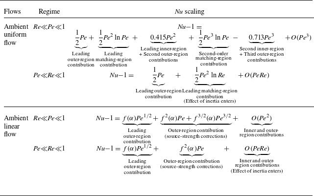
 Pe
 Nu

 ⟨x12⟩
 Sl
 t∼O(Sl−1)
 ⟨x12⟩
 α=0.1
 t∼O(Sl−1)

 (Nu(θ)−Nu(0))/(Nu(π/2)−Nu(0))
 θ
 Pe
 θ=(π/2)
 θ
 Nu
 θPe1/2
 Pe−1/2)
 Nu((π/2);θ)
 Usinθ
 Nu
 O(Pe−1/2)
 Pe

 T
 κ=4
 10
 C=1
 C
 0
 ∞
 t=T/4
 Nu
 α
 Pe=0.1
 O(bPeb−1/2)

 Pe

 ϵ=−1
 ϵ=−1.5
 ϵ=−1.95
 C−τ
 x1−x2
 ϵ→−2
 Nu/Pe1/3
 Nu/Pe~1/2
 Pe~=Pe/(1+λ)
 ϵ
 Pe∗=(E:E)1/2(2a)2/D

 x3=0
 α=0.15
 α^=1.48
 α=0
 α^=2
 α=−0.4;α^=4.67
 x2
 (±[(1+α)/(2α)]1/5,0)
 x1

 Nu−Pe
 α
 Nu
 A(=α^/2)
 α→1
 A→∞
 Pe
 Nu
 5.73

 Re
 Re=1
 Pe=3000
 Nu
 Pe
 Re→0
 Nu
 Pe
 Sc
 Pr
 Sc
 Re
 Nu
 4.5
 Nu

 Nu¯/Pe1/3
 Ep
 κ=4
 α^=26
 θω∈[0,π/2]
 θω=81.82∘
 60.21∘
 45∘
 κ=4)
 κ=0.25

 Pe

 {ϵ,α^}≡{−0.75,0.4}
 {−0.75,1.5}
 λ=1
 1.2
 1.05
 1.01

 Δ′=([−(2+ϵ)2+α^′2][4(1+ϵ−2ϵ2)−α^′2]2/16)
 α^′=α^(1+λ)
 ϵ=−0.75
 α^c′=1.25
 C−τ
 α^′=0.4
 α^′=1.5
 Nu/Pe1/2
 [α^,ϵ]
 λ=1

 Re=0
 λ=λc
 α,λ
 A≡(0.75,0)
 B≡(0.5,2)
 C≡(0.25,8)
 D≡(0.1,1000)
 Nu
 Pe
 λ→λc+
 Nu/Pe1/2
 α
 λ
 Pe→∞
 λ<λc
 λ>λc

 Nu/Pe1/2
 θω=1/2cos−1[−(16+(α^′)2)/(3(α^′)2)];α^′∈[12,∞)
 α^′−θω
 λ=1
 Δ′
 R′
 α^′
 θω=1.05
 α^′≈5.58

 α^=6
 α^=42,ϵ=−2,θω=π/3,ϕω=0
 v3
 Ei(i=1 to 3)

 F
 R
 Pe
 Nu∝Pe1/2
 Pe
 Nu∝Pe1/3
 Nu∝Pe1/2

 292μm s−1
 340μm s−1

 Nu
 Pe
 3/5
 Pe=∞
 Nu
 τ(=tD/a2)
 Pe
 Pe
 −1/2

 Ca=0
 α=1
 λ
 α=0.5
 λ=1
 S0−S4
 Nu−Pe

 θω=36∘
 λ=1
 α^=
 0.1
 0.5
 2
 8
 x1−x3

 Nu/Nu0−1
 Pe
 α^=0.1
 Pe2
 θω=45∘
 63∘
 Nu∝Pe1/2
 Pe≫1
 (1−r)Pe1/2

 Nu−Pe
 Ca
 Ca=0.001
 Nu
 PeCa
 λ=1

 Nu
 PeCa
 α=0
 0.25
 0.5
 0.75
 Nu
 PeCa
 (0,0.5,0.1)
 α=0.5
 λ=1
 Ca=0.005
 Ca


