1 Introduction
Fluid flow past multiple circular cylinders has been studied extensively due to its relevance to many engineering applications. The simplest configuration of multiple cylinders is two cylinders that are parallel to each other in steady flows. Zdravkovich (Reference Zdravkovich1977) and Sumner (Reference Sumner2010) presented detailed reviews of flow past two parallel circular cylinders in different arrangements. The interesting phenomenon for the wake flow of two parallel cylinders in side-by-side arrangement is that, if the gap between the two cylinders is small enough, the flow through the gap biases towards one cylinder, forming a narrow wake behind one cylinder and a wide wake behind the other cylinder (Williamson Reference Williamson1985; Zdravkovich Reference Zdravkovich1987; Zhou, Zhang & Yiu Reference Zhou, Zhang and Yiu2002; Alam, Moriya & Sakamoto Reference Alam, Moriya and Sakamoto2003; Afgan et al. Reference Afgan, Kahil, Benhamadouche and Sagaut2011). Studies of flow past two tandem cylinders have been focused on the effects of the gap on the vortex shedding from the upstream cylinder, which occurs only when the gap between the two cylinders are large enough (Zdravkovich Reference Zdravkovich1987; Carmo, Meneghini & Sherwin Reference Carmo, Meneghini and Sherwin2010a ,Reference Carmo, Meneghini and Sherwin b ; Liu et al. Reference Liu, Lu, Teng, Zhao and Tang2014). The critical gap above which the vortex shedding from the upstream cylinder occurs is dependent on the Reynolds number. If two parallel cylinders are in a staggered arrangement, it was found that the flow is affected by the combination of the gap and the direction of the flow (Gu & Sun Reference Gu and Sun1999; Sumner, Price & Paidoussis Reference Sumner, Price and Paidoussis2000; Sumner, Richards & Akosile Reference Sumner, Richards and Akosile2005; Carmo et al. Reference Carmo, Sherwin, Bearman and Willden2008; Tong, Cheng & Zhao Reference Tong, Cheng and Zhao2015).
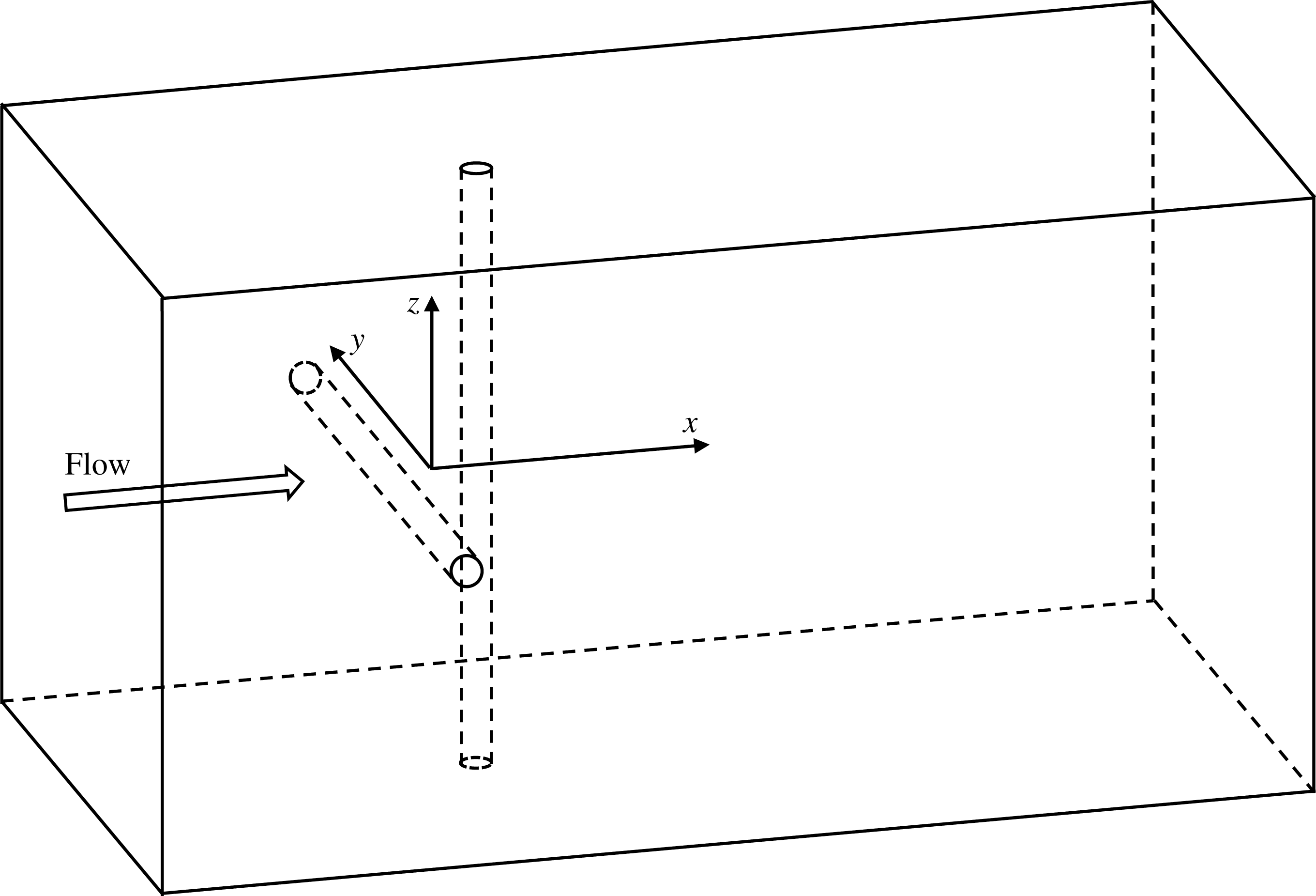
Sketch of flow past two crossing cylinders in cruciform arrangement.

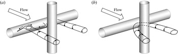
In some engineering applications, two circular cylinders are perpendicular to each other, forming a so-called cruciform arrangement, as shown in figure 1. Examples of two circular cylinders in cruciform arrangement include the pipes in heat exchangers, truss structures in wind or water flows, offshore pipeline crossing, etc. The number of studies of flow past two cylinders in a cruciform arrangement with a gap between them is far less than that of flow past two parallel cylinders. Zdravkovich (Reference Zdravkovich1983) conducted an experimental study of flow past two cylinders in cruciform arrangement and found longitudinal vortices were formed by strong secondary flow along the rear side of the upstream cylinder. Through flow visualization in experiments, Shirakashi et al. (Reference Shirakashi, Bae, Sano and Takahashi1994) reported that the flow near the crossing region between the two cylinders is in the form of trailing vortices (TV) if the gap-to-diameter ratio (defined as
 $G$
) is between 0 and 0.25 and in the form of necklace vortices (NVs) if
 $G$
is between 0.25 and 0.5 (see figure 2). The NVs were originally defined as horseshoe vortices in the study of flow past two square-section cylinders perpendicular to each other (Fox Reference Fox1992). The NV forms periodically around the downstream cylinder and causes the low frequency oscillation of the fluid velocity. Since then, the TV and NV have been the focus of several studies of flow past two cylinders in cruciform arrangement (Nguyen et al.
Reference Nguyen, Koide, Takahashi and Shirakashi2010, Reference Nguyen, Koide, Yamada, Takahashi and Shirakashi2012).
Kato et al. (Reference Kato, Koide, Takahashi and Shirakash2012) investigated the vortex-induced vibration (VIV) of an elastically mounted horizontal circular cylinder with a stationary downstream vertical strip plate. It was found that whether the VIV response is enhanced or suppressed by the plate depends on the gap between the cylinder and the plate. Nguyen et al. (Reference Nguyen, Koide, Yamada, Takahashi and Shirakashi2012) carried out similar experiments with the downstream strip plated replaced by a circular cylinder. Deng, Ren & Shao (Reference Deng, Ren and Shao2007) numerically simulated the VIV of the downstream cylinder with a stationary upstream cylinder in cruciform arrangement. It was found that the peak amplitude is smaller than that of an isolated cylinder but the resonant region is wider.
All the existing studies of flow past two cylinders in cruciform arrangement have been focused on the flow patterns near the crossing between the two cylinders. No attention has been paid to the global vortex shedding flow pattern in the wake of the two cylinders or the effect of the crossing on the fluid force. In this study, steady flow past two circular cylinders in cruciform arrangement is studied using three-dimensional numerical simulations. The study is aimed at finding out the effect of the crossing on the Kármán vortex streets in the wake of the two cylinders and the force distribution along each cylinder. The Navier–Stokes equations are solved using the upwind finite element method. The length of each cylinder is 42 diameters in the numerical simulations. Simulations are performed for Reynolds numbers ranging from 100 to 500 and gap to diameter ratios of 0.5, 1, 2 and 4.
(a) Sketch of the trailing vortex (TV) and (b) necklace vortex (NV) reproduced based on Nguyen et al. (Reference Nguyen, Koide, Takahashi and Shirakashi2010).

2 Numerical method
For the purpose of convenience, the upstream and downstream cylinders are defined as UC and DC, respectively. In figure 1, a Cartesian coordinate system is defined with its origin located at the centre of the gap between the two cylinders, the
 $x$
-axis pointing the flow direction and the
 $y$
- and
 $z$
-axes parallel to the UC and DC, respectively. The flow direction is perpendicular to both cylinders.
The governing equations for simulating the incompressible viscous fluid flow are the three-dimensional (3-D) Navier–Stokes (NS) equations. The velocity, the length, the time and the pressure are non-dimensionalized by the free-stream velocity (
 $U$
), the diameter of the cylinder (
 $D$
),
 $D/U$
and
 $\unicode[STIX]{x1D70C}U^{2}$
, respectively, where
 $\unicode[STIX]{x1D70C}$
is the fluid density. The dimensionless NS equations are
 $$\begin{eqnarray}\displaystyle & \displaystyle \frac{\unicode[STIX]{x2202}u_{i}}{\unicode[STIX]{x2202}x_{i}}=0, & \displaystyle\end{eqnarray}$$
 $$\begin{eqnarray}\displaystyle & \displaystyle \frac{\unicode[STIX]{x2202}u_{i}}{\unicode[STIX]{x2202}t}+u_{j}\frac{\unicode[STIX]{x2202}u_{i}}{\unicode[STIX]{x2202}x_{j}}=-\frac{\unicode[STIX]{x2202}p}{\unicode[STIX]{x2202}x_{i}}+\frac{1}{Re}\frac{\unicode[STIX]{x2202}^{2}u_{i}}{\unicode[STIX]{x2202}x_{j}\unicode[STIX]{x2202}x_{j}}, & \displaystyle\end{eqnarray}$$
where
 $x_{i}$
(
 $x_{1}=x$
,
 $x_{2}=y$
and
 $x_{3}=z$
) represents the Cartesian coordinates,
 $u_{i}$
is the fluid velocity in the
 $x_{i}$
-direction,
 $t$
is time and
 $p$
is pressure. The Reynolds number
 $Re$
is defined as
 $Re=UD/\unicode[STIX]{x1D708}$
, where
 $\unicode[STIX]{x1D708}$
is the kinematic viscosity of the fluid.
The non-dimensional gap between the two cylinders (i.e. the gap distance to diameter ratio) is defined as
 $G$
. A rectangular computational domain with a length of
 $45+G$
in the
 $x$
-direction, a width of 42 in both the
 $y$
- and
 $z$
-directions is used. To minimize the end effects, the results within one diameter of the end of each cylinder are not considered when analysing the results. The distance between the upstream cylinder and the inlet boundary is 15.
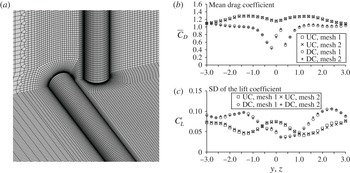
The boundary conditions are specified as follows. On the left boundary, a uniform velocity is given and the pressure gradient in the streamwise direction is zero. On the right boundary, the gradient of the velocity in the streamwise direction and the pressure are zero. On the four side boundaries, the velocity component and the gradient of the pressure in the normal direction of the boundary are zero. On the cylinder surfaces, no-slip boundary condition is applied, i.e. the velocity and the pressure gradient normal to the cylinder surface is zero. Figure 3(a) shows the computational mesh for
 $G=0.5$
. The computational domain is divided into 11.5 million and 14.0 million hexahedral finite elements for
 $G=0.5$
and 4, respectively. The mesh in the wake of the whole span of each cylinder is consistently dense to ensure a good resolution of wake flow. Parallel calculations based on message passing interface (MPI) are conducted on the supercomputer facilities provided by Intersect Ltd., NSW, Australia.
(a) Computational mesh for
 $G=0.5$
and (b) comparison between the force coefficients from the two meshes.

The numerical model used in the present study is the same as the one developed in our previous publications. Zhao et al. (Reference Zhao, Thapa, Cheng and Zhou2013) demonstrated the validity of the numerical model in simulating three-dimensional steady flows over a circular cylinder for Reynolds numbers ranging from 100 to 1000. Based on the present model, Thapa et al. (Reference Thapa, Zhao, Cheng and Zhou2015a
) successfully predicted the biased wake flow behind two side-by-side parallel cylinders at
 $Re=500$
and obtained excellent agreements between the computed force coefficients and the experimental data. The validation of the numerical model in the simulation of flow past two circular cylinders of different diameters at
 $Re=500$
was conducted by Thapa et al. (Reference Thapa, Zhao, Cheng and Zhou2015b
). The density of the computational mesh used in this study is the same as the one used in Thapa et al. (Reference Thapa, Zhao, Cheng and Zhou2015b
), where detailed mesh dependency studies have been provided for
 $Re=500$
. A mesh dependency study is conducted by performing an extra simulation for
 $G=0.5$
and
 $Re=500$
with a denser mesh (referred to as mesh 2). The density of the denser mesh is approximately twice that of the normal mesh in the region of
 $|y|\leqslant 5$
and
 $|z|\leqslant 5$
. The sectional drag and lift coefficients are defined as
 $C_{D}=2F_{D}/(\unicode[STIX]{x1D70C}DU^{2})$
and
 $C_{L}=2F_{L}/(\unicode[STIX]{x1D70C}DU^{2})$
, where
 $F_{D}$
and
 $F_{L}$
are the sectional drag and lift forces, respectively, which are obtained by integrating the pressure and shear stress along the circumference of the section. Figure 3(b) shows the comparison between the statistic values of the force coefficients from the two meshes, where
 $\bar{C}_{D}$
and
 $C_{L}^{\prime }$
stand for the mean drag coefficient and the standard deviation of the lift coefficient, respectively. Mesh 1 refers to the mesh that is used for all the simulations for
 $G=0.5$
in this study. It can be seen that the force coefficients obtained from the two meshes are very close to each other. Because the interaction between the two cylinders,
 $C_{L}^{\prime }$
of both cylinders are smaller than that of an isolated single cylinder.
3 Numerical results
3.1 Vortex types near the crossing
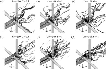
To compare the simulated flow modes with the experimental flow visualization, three-dimensional streamlines are used to identify the flow modes near the gap. Figure 4 shows the streamlines for some typical cases. The streamlines start from positions two diameters upstream of the UC in the
 $x{-}z$
plane. The majority of the existing experimental studies of flow over two cylinders in a cruciform arrangement paid attention to the local flow near the gap between the two cylinders with small gap ratios (
 $G<0.5$
). The previous studies show that the TV mode only occurs when the gap is very small, where vortices do not form immediately behind the centre of the UC. In the NV mode, vortices form between the two cylinders but there is not vortex shedding.
In figure 4(a), where the gap between the two cylinders is 0.5 and
 $Re=100$
, the streamlines diverge from the centre of the gap and point towards the two ends of the UC. They form vortices at a distance from the gap, forming TV vortices at two sides of the DC. As the Reynolds number increases to 500 and the gap remains at
 $G=0.5$
, it can be seen in figure 4(d) that a vortex in the shape of a necklace is generated between the two cylinder centres, forming a NV vortex. When the gap is increased up to 2 with the same
 $Re=500$
, vortex shedding occurs behind the centre of the UC.
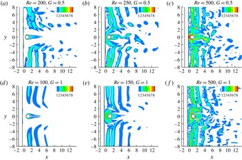
To further assist the identification of the TV and NV, the contours of the magnitude of the vorticity in the
 $x{-}y$
plane for several representative cases are shown in figure 5. The vorticity
 $\unicode[STIX]{x1D714}$
is defined as
 $\unicode[STIX]{x1D714}=(\unicode[STIX]{x1D714}_{x}^{2}+\unicode[STIX]{x1D714}_{y}^{2}+\unicode[STIX]{x1D714}_{z}^{2})^{1/2}$
, where
 $\unicode[STIX]{x1D714}_{x}$
,
 $\unicode[STIX]{x1D714}_{y}$
and
 $\unicode[STIX]{x1D714}_{z}$
are the vorticity components in the
 $x$
-,
 $y$
- and
 $z$
-directions, respectively. When
 $(Re,G)=(200,0.5)$
, TV can be seen at the two sides of the DC in figure 5(a) and the vortices between the two cylinders are too weak to be observed. When
 $(Re,G)=(250,0.5)$
and (150, 1), a NV forms and surrounds the upstream part of the DC. The TV flow pattern is very similar to the TV reported in the previous experimental studies (Shirakashi et al.
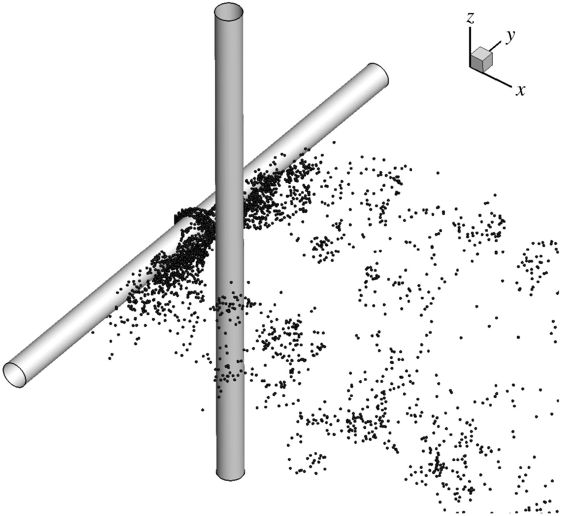
Reference Shirakashi, Bae, Sano and Takahashi1994). Figure 6 shows an example of the flow visualization of the NV using streaklines for
 $Re=500$
and
 $G=0.5$
. The NV observed in figure 6 is in a similar pattern as the flow visualization in the physical test (i.e. the figure 4 in Kato et al.
Reference Kato, Koide, Takahashi and Shirakash2012).
Streamlines near the crossing between the two cylinders.

Contours of the magnitude of the vorticity on the
 $x{-}y$
-plane.

Streaklines near the crossing for
 $Re=500$
and
 $G=0.5$
.

The formation mechanism of the NV around the DC is the same as that of the horseshoe vortex around the base of a vertical cylinder mounted on a horizontal plane boundary, for example bridge piers in hydraulic engineering (Dargahi Reference Dargahi1989). In the study of flow past two crossing square cylinders, Fox (Reference Fox1992) defined the NV as the horseshoe vortex. While the horseshoe vortex near the base of a bridge pier originates from the shear layer developed on the bottom boundary, the NV for two crossing cylinders is generated by the free shear layers from the two sides of the upstream cylinder. When the shear layers approach the front surface of the DC, a pressure gradient towards the centre of the front surface of the DC makes the streamlines converge in front of the DC. The downward flow from the top part of the DC and upward flow from the bottom part of the DC meet and form two vortices surrounding the upstream half of the DC, as shown in figure 4(d,e).
In the previous experimental studies, the flow near the gap was found to be in the trailing vortex (TV) mode when
 $G=0.08$
and necklace vortex (NV) mode when
 $G=0.28$
(Kato et al.
Reference Kato, Koide, Takahashi and Shirakash2012; Koide et al.
Reference Koide, Takahashi, Shirakashi and Salim2017). The identified gaps for the TV and NV modes in this work are different from those observed in the previous experimental data. This is mainly because that the experimental studies were conducted at much higher Reynolds numbers. For example, the Reynolds number used in Kato et al. (Reference Kato, Koide, Takahashi and Shirakash2012) ranges from
 $3\times 10^{3}$
to
 $2.2\times 10^{4}$
. The effect of the Reynolds number on the flow pattern near the gap can be seen in figure 5. Taking
 $G=0.5$
as an example, the flow near the gap is in the TV mode at
 $Re=200$
(figure 5
a) and NV mode at
 $Re=250$
and 500 (figure 5
b,c). The effect of the Reynolds number can also been seen in figure 4. As the gap ratio is increased to 2 with larger
 $Re=500$
, vortex shedding from the centre of the UC occurs and neither TV nor NV exists, as shown in figure 4
f). However, the vortex in the gap between the two cylinder is still a NV at
 $Re=100$
and
 $G=2$
(figure 4
c).
In this study, the flow mode developed in the gap is named the mode of vortex shedding in the gap (SG) if the vortices are shed from the centre of the UC. Table 1 lists types of the vortices near the gap for all the simulated cases. It can be seen that if the Reynolds number is constant, TV occurs at a very small gap ratio, NV occurs at an intermediate gap ratio and SG occurs when the gap is large enough. The boundary gaps between different vortex types decrease with increasing Reynolds number. All the three vortex types are observed at
 $Re\leqslant 200$
, but no TV is observed for
 $G\geqslant 0.5$
at
 $Re\leqslant 250$
. It is expected that the range of the gap ratio for TV is less than 0.5 as
 $Re\geqslant 250$
. The flow in the gap between the two cylinders is dependent on the recirculation length in the wake of the UC, which is a function of the Reynolds number. The non-dimensional recirculation length was found to decreases from 3 to 1 as the Reynolds number increases from 50 to 200 and does not change between
 $Re=200$
and 300 (Lima E Silva, Silva-Neto & Damasceno Reference Lima E Silva, Silva-Neto and Damasceno2003). It can be seen that the variations of the boundary
 $Re$
between TV and NV and that between NV and SG follow the same trend as the variation of the recirculation length with
 $Re$
.
Classification of the vortices near the crossing between the two cylinders.

3.2 Wake vortex shedding
Vortex shedding from the cylinder occurs outside the centre part of each cylinder if the Reynolds number falls into the vortex shedding regime (for a single cylinder), regardless of the vortex pattern in the gap. However, it is expected that the flow near the crossing point affects the vortex shedding flow pattern. The 3-D vortex shedding flow structure is firstly presented by the iso-surface of the second eigenvalue
 $\unicode[STIX]{x1D706}_{2}$
of the tensor
 $\unicode[STIX]{x1D733}^{2}+\unicode[STIX]{x1D734}^{2}$
, where
 $\unicode[STIX]{x1D733}$
and
 $\unicode[STIX]{x1D734}$
are the symmetric and the anti-symmetric parts of the velocity-gradient tensor, respectively. The detailed method for determining
 $\unicode[STIX]{x1D706}_{2}$
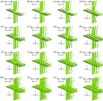
can be found in Jeong & Hussain (Reference Jeong and Hussain1995). Figure 7 shows the iso-surfaces of
 $\unicode[STIX]{x1D706}_{2}=-0.2$
for different gap ratios and Reynolds numbers. The vortex flow structure at a low Reynolds number of 150 is very similar to those observed by Deng et al. (Reference Deng, Ren and Shao2007), who conducted numerical simulations of flow past two cylinders with a length of 12 diameters at
 $Re=150$
. In the following discussion it can be seen that a length of 40 diameters is necessary to ensure that the effects of the crossing can be accurately predicted.
Small scale vortices can be clearly seen near the gap between the two cylinders when
 $Re=150$
, indicating that the wake flow is transitioning from laminar to turbulent flow. The transition of wake flow from laminar to turbulent for a single cylinder occurs at approximately
 $Re=180{-}200$
. When
 $Re=150$
, the flow is weakly turbulent only near the gap, except at
 $G=2$
, where the flow in the wake of the top part of the DC is weakly turbulent. The turbulent flow region extends from the cylinder centres towards the cylinder ends with increasing Reynolds number. When the Reynolds number is increased to 200, the flow in the whole wake zone becomes turbulent. Based on the size of small scale vortices, it can be seen that the turbulent length scale decreases significantly as the Reynolds number is increased from 200 to 500.
Iso-surfaces of
 $\unicode[STIX]{x1D706}_{2}=-0.2$
for different Reynolds numbers and gap ratios.

An interesting phenomenon observed in figure 7 is that the vortices in the wake of either the UC or the DC are inclined relative to the cylinder in some cases. For example, at
 $Re=100$
,
 $G=2$
and 4 (figure 7
c,d), the vortex shedding near the centre part of each cylinder lags the vortex shedding near the two ends of the cylinder, forming a vortex street in a K-shape. This inclined vortex shedding mode is called K mode in this study. In the cases of
 $Re=100$
,
 $G=0.5$
and 1 (figure 7
a,b), the vortex shedding mode is defined as a parallel vortex shedding mode, or P mode, because the vortices are parallel to the cylinders except near the crossing point. Near the crossing, where the spanwise vortices are very weak, the streamwise vortices in the forms of TV and NV can be observed for
 $Re=100$
and 150 in figure 7, but not as clearly as those in figures 4 and 5. When the Reynolds number is greater than 200, the streamwise TV and NV cannot be seen clearly in figure 7 because they are overwhelmed by the streamwise vortices due to the three-dimensionality. The streamwise vortices in the wake of a cylinder form when the Reynolds number is in the transition regime (
 $Re=200$
and 250) due to the three-dimensionality, and dominate the wake flow when the Reynolds number is in the turbulent regime (
 $Re=300$
and 500) (Williamson Reference Williamson1989). Some K mode vortex shedding can be seen when
 $Re=200$
and 250, for example when
 $Re=250$
and
 $G=2$
. As for
 $Re=300$
and 500, it is difficult to identify the K mode because of the strong influence of the streamwise vortices.
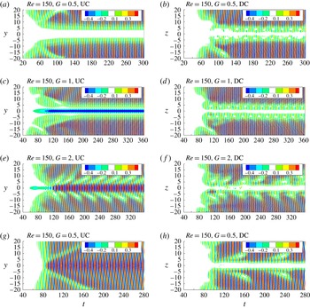
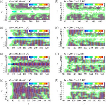
Contours of the sectional lift coefficient in the
 $y$
–
 $t$
plane for UC and
 $z$
–
 $t$
plane for DC for
 $Re=150$
and different gap ratios.

Contours of the sectional lift coefficient in the
 $y$
–
 $t$
plane for UC and
 $z$
–
 $t$
plane for DC for
 $Re=200$
and different gap ratios.

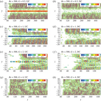
Contours of the sectional lift coefficient in the
 $y$
–
 $t$
plane for UC and
 $z$
–
 $t$
plane for DC for
 $Re=500$
and different gap ratios.

An alternative way of identifying the pattern of vortex shedding is to analyse the distribution of the force coefficient along the cylinder spans, since the fluid forces are highly correlated to the vortex shedding. To help in identifying the vortex shedding mode and understanding the time histories of the flow, the contours of the sectional lift coefficient in the
 $y$
–
 $t$
plane for UC and
 $z$
–
 $t$
plane for DC for
 $Re=150$
, 200 and 500 are presented in figures 8–10, respectively. The three Reynolds numbers in figures 8–10 correspond to the laminar, transition and turbulent flow regimes, respectively.
If the vortex shedding from a cylinder is in P mode, for example,
 $Re=150$
,
 $G=0.5$
and 1 (figure 8
a), the contours of the sectional lift coefficient of a cylinder are generally parallel to the axis of the cylinder except near the centre of the cylinder. If the vortex shedding is in a K mode, for example,
 $Re=150$
and
 $G=2$
(figure 8
e), the contours are inclined with respect to the axis of a cylinder (
 $y$
-axis for UC and or
 $z$
-axis for DC). The disconnection of the contours near the centre of the both cylinders in figure 8(d–f) is caused by the dislocation of the vortices.
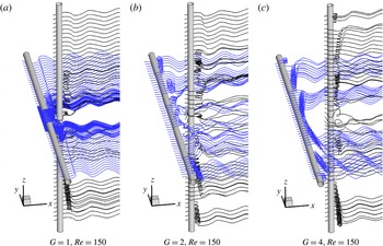
Three-dimensional streamlines for
 $Re=150$
.

The correlation between the disconnection of the contours in figure 8 and the vortex dislocation can be further evidenced by comparing the contours of the lift coefficients in figure 8 and the 3-D streamlines shown in figure 11. The dislocation of vortices that can be clearly seen in the wake of both cylinders in figure 11(b) corresponds to the disconnection in the contours of the lift coefficient in figure 8(c). In figure 8(c) the disconnection is found to start at the two sides of the cylinder in an alternating fashion. The dislocation of the vortices is found for all the cases where the SG mode occurs and the wake vortex is in K mode. The K mode wake vortices are not parallel to the cylinders and disconnection locations of the vortices start from the crossing points between a cylinder and a streamwise vortex, and progress towards the ends of the cylinder. When
 $Re=150$
and
 $G=2$
, the dislocation disappears after it progresses for a short distance. When the Reynolds number is increased to 200, the dislocation of the vortices can progress further towards the ends of a cylinder, as shown in figure 8(c). It should be noted that the occurrence of the dislocation of the vortices for
 $Re=200$
is because of not only the K mode vortex shedding but also the transition of the wake flow from two to three dimensions. Wake vortex dislocation is a typical phenomenon of wake flow in the 2-D–3-D transition flow regime (Williamson Reference Williamson1989).
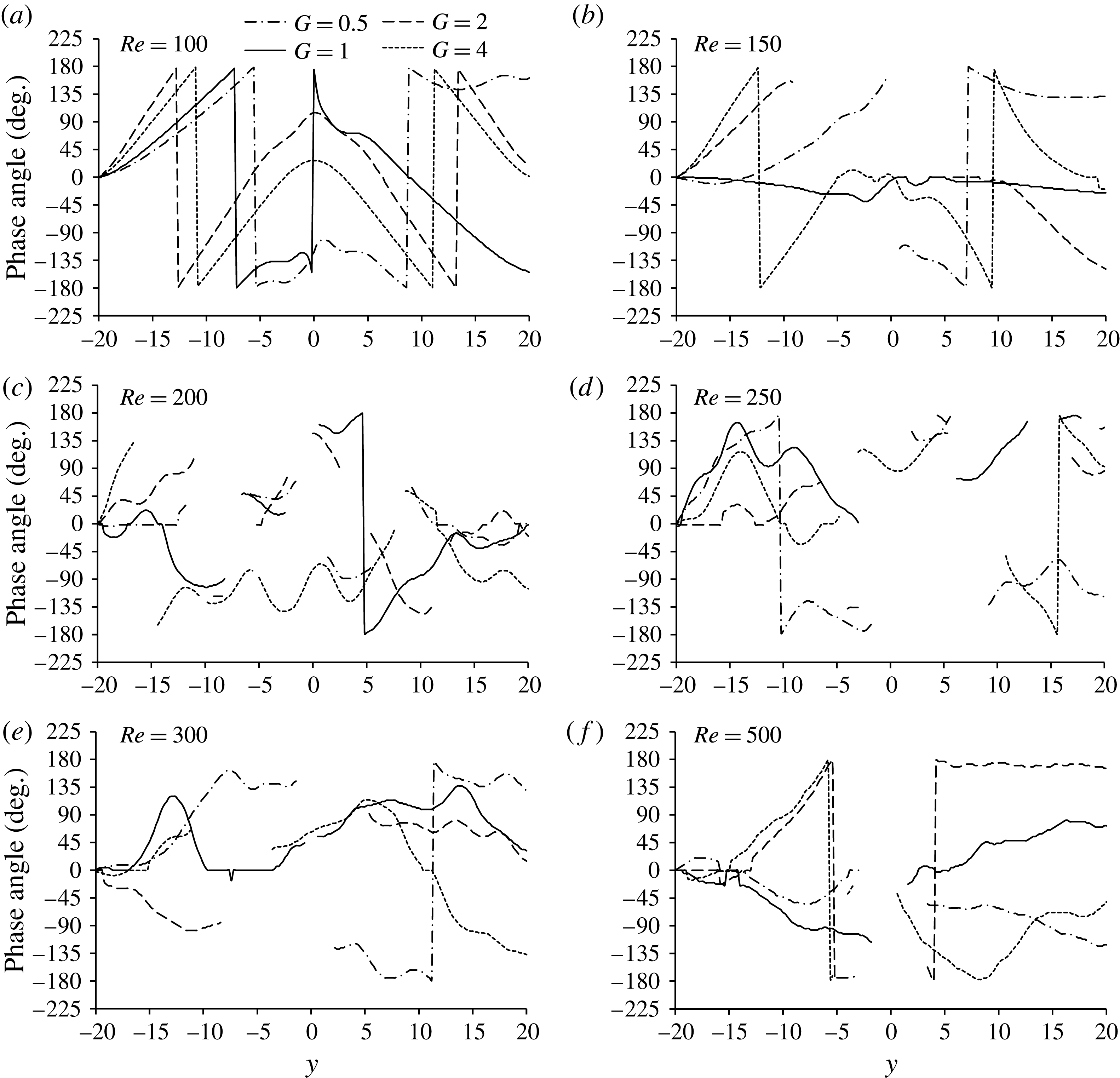
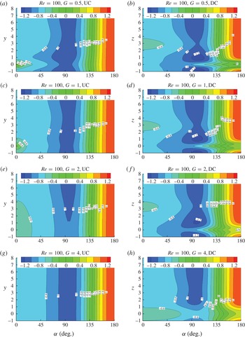
The inclination of the K mode wake vortex street makes the phase angle of the oscillatory lift coefficient vary along the cylinder span. To quantify this phenomenon, the phase angle of the sectional lift coefficient is calculated, and its distribution along the UC is presented in figure 12. The method for determining the phase difference between the lift coefficients at two sections is the same as the one used by Zhao et al. (Reference Zhao, Kaja, Xiang and Cheng2016). Firstly, the cross-correlation coefficient between two oscillatory lift coefficients at two sections of the cylinder, denoted by
 $C_{L1}$
(
 $t$
) and
 $C_{L2}$
(
 $t$
), respectively, is calculated using
 $n$
periods of data by
 $C_{12}(\unicode[STIX]{x1D70F})=1/nT\int _{0}^{nT}[C_{L1}(t)-\bar{C}_{L1}]\cdot [C_{L2}(t+\unicode[STIX]{x1D70F})-\bar{C}_{L2}]\,\text{d}t/(C_{L1}^{\prime }C_{L2}^{\prime })$
, where
 $T$
is the oscillation period of the lift coefficient and
 $\unicode[STIX]{x1D70F}$
is the time lag. The oscillation period of the cross-correlation coefficient is the same as the period of the lift coefficient, and the maximum value of the correlation coefficient
 $C_{12,max}$
is nearly 1 if both
 $C_{L1}$
and
 $C_{L2}$
oscillate nearly sinusoidally with a same frequency. If the time lag corresponding to
 $C_{12,max}$
is defined as
 $\unicode[STIX]{x1D70F}_{m}$
, the time lag can be converted to the phase difference by
 $\unicode[STIX]{x1D719}=2\unicode[STIX]{x03C0}\unicode[STIX]{x1D70F}_{m}/T$
in radians and
 $\unicode[STIX]{x1D719}=360\unicode[STIX]{x1D70F}_{m}/T$
in degrees. The reference point is
 $y=-20$
when the phase angles of UC are calculated, i.e. all the phase angles are relative to the phase at
 $y=-20$
. The reference point for the phase angles of DC is
 $z=-20$
. Ten periods of numerical data are used to calculate the phase of the lift coefficient. If the lift forces at two sections are not correlated well (
 $C_{12,max}<0.8$
), the phase angle is meaningless and is not calculated. Poor correlation occurs at locations where dislocation of the vortices occurs or near the gap if the vortex shedding does not exist. It should be noted that the jump of the phase angle between
 $-180^{\circ }$
and
 $180^{\circ }$
is not a discontinuation.
If the Reynolds number is in the laminar regime (
 $Re=100$
and 150), the wake vortices are continuous and the phase angle has good continuity except at the centre of the cylinder.
 $Re=200$
and 250 are in the transition regime from two to three dimensional flows. It is well known that the dislocation of wake vortices is one of the key characteristics of wake flow in the transition regime. Because of the severe dislocation of the wake vortices at
 $Re=200$
and 250, the correlation of the lift coefficient along the UC is very poor and the phase angle cannot be calculated at many sections, as shown in figure 12(c,d). When the Reynolds number is increased to 300, the continuity of the phase angle along the cylinder span recovers, but the phase angle oscillates along the cylinder span. When
 $Re=500$
, the oscillation of the phase angle along the cylinder span becomes weak.
Variation of the phase angle of the lift coefficient along the UC.

The inclination of the wake vortices is quantified by calculating the non-dimensional change rate of the phase angle in the spanwise direction of a cylinder, namely,
 $\text{d}\unicode[STIX]{x1D703}/\text{d}y$
and
 $\text{d}\unicode[STIX]{x1D703}/\text{d}z$
for the UC and DC, respectively, which represent the change of
 $\unicode[STIX]{x1D703}$
in unit length of cylinder. The change rates of the phase angle for
 $Re=100$
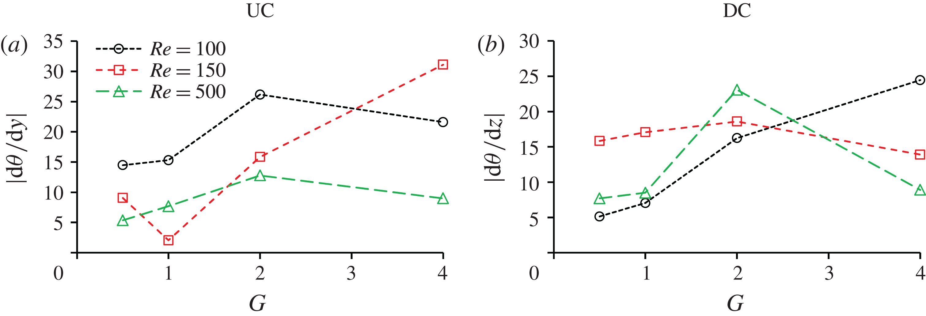
, 150 and 500 for both cylinders are shown in figure 13. The change rate of
 $\unicode[STIX]{x1D703}$
in the spanwise direction is calculated based on linear curve fitting by using the data of
 $\unicode[STIX]{x1D703}$
between
 $5\leqslant |y|\leqslant 20$
for UC and 5
 ${\leqslant}|z|\leqslant$
20 for DC. The results for
 $Re=200$
and 250 are not included in the figure because the phase angle
 $\unicode[STIX]{x1D703}$
is severely discontinuous in the spanwise direction. Considering that the values of
 $\text{d}\unicode[STIX]{x1D703}/\text{d}y$
(or
 $\text{d}\unicode[STIX]{x1D703}/\text{d}z$
) on the two sides of the cylinder have opposite signs, the absolute value is shown in figure 13. In the cases where
 $|\text{d}\unicode[STIX]{x1D703}/\text{d}y|$
or
 $|\text{d}\unicode[STIX]{x1D703}/\text{d}z|$
on one side is very different from that on the other side of a cylinder (for example,
 $G=4$
and
 $Re=150$
in figure 12
b), the maximum absolute value of the two sides is shown in figure 13.
Variation of the change rate of the phase angle of the lift coefficient along the cylinders.

List of wake vortex shedding modes.

In general the change rates of the phase angle for
 $G/D=0.5$
and 1 are smaller than those for
 $G/D=2$
and 4. Although the phase angle always varies along the cylinder span for all the simulated cases, the inclination of the wake vortices can be identified in the flow visualization either from the 3-D iso-surface of
 $\unicode[STIX]{x1D706}_{2}$
in figure 7 or the signal of the sectional lift coefficients in figures 8–10 only if the change rate of the phase angle is greater than
 $10^{\circ }$
per cylinder diameter length. In this paper, the vortex shedding mode is defined as the K mode only if the inclination angle can be clearly identified in the flow visualization, i.e.
 $\text{d}\unicode[STIX]{x1D703}/\text{d}y$
or
 $\text{d}\unicode[STIX]{x1D703}/\text{d}z>10^{\circ }$
.
Table 2 lists all the identified vortex shedding modes. The vortex shedding of each case is represented by two modes connected by a hyphen, which are the vortex shedding modes of the UC and DC, respectively. For example, K–P means that the vortex shedding behind the UC is in a K mode while that of the DC is in a parallel mode (P mode). It is found that the flow is always in K mode if
 $G=2$
for all the examined Reynolds numbers. At
 $Re=100$
, the flow is in K mode either behind both cylinders or just behind the UC, depending on the gap ratio. Table 2 shows that the K mode is likely to occur in two conditions: (i) a small Reynolds number and (ii) a gap ratio slightly greater than the critical gap ratio between NV and SG, i.e.
 $G=2$
.
That the K mode is likely to occur at
 $G=2$
can be explained by the influence of vortex flow in the gap on the global vortex shedding. The K mode is found only when the spanwise vortices generated from the UC (in the
 $y$
-direction) are continuous. When the gap is smaller than
 $G=2$
, vortices disconnect in the gap, because vortex shedding does not occur at the centre of the UC (see figure 14) but occurs at the two sides of the centre. When the
 $G=2$
, vortex shedding from the centre of the UC occurs. However, the vortex shedding from the centre of the UC lags that at the two sides of the centre because the front surface of the DC delays the vortex shedding from the UC. The delay of the vortex shedding at the centre of the UC results in a K mode vortex shedding pattern. When the gap is large, the effect of DC on the vortex shedding from the UC becomes weak and the K mode vortex shedding flow disappears. As mentioned above,
 $\text{d}\unicode[STIX]{x1D703}/\text{d}y$
and
 $\text{d}\unicode[STIX]{x1D703}/\text{d}z$
are correlated to the degree of the inclination of the vortices. They are small when
 $G$
is small because the vortex shedding is in the parallel shedding mode. Because of the strong inclination of the wake vortices in the K mode vortex shedding,
 $\text{d}\unicode[STIX]{x1D703}/\text{d}y$
for
 $G=2$
is significantly greater than those for
 $G=0.5$
and 1 for all the Reynolds numbers. When the K mode vortex shedding disappears as the result of increasing
 $G$
,
 $\text{d}\unicode[STIX]{x1D703}/\text{d}y$
decreases accordingly.
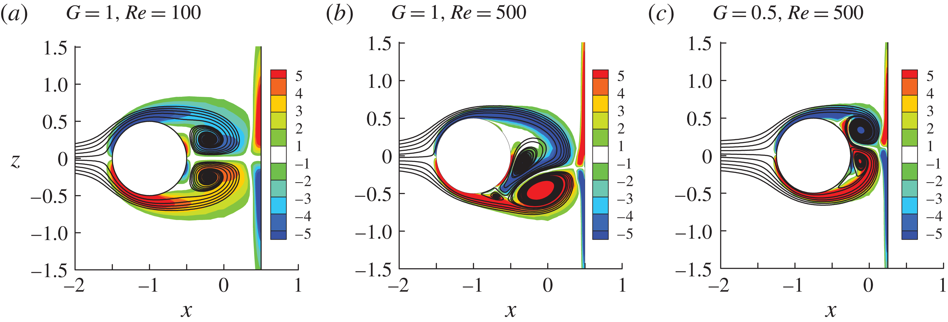
Another interesting phenomenon observed in figures 8–10 is that the average lift coefficient at the centre of the UC is non-zero. This happens when the gap ratio
 $G=1$
for
 $Re\in [150,500]$
, and
 $G=0.5$
with
 $Re=500$
.
 $G=1$
is slightly smaller than the critical value between NV and SG. The occurrence of non-zero lift coefficient is due to the asymmetric flow in the gap between the two cylinders, as shown in figure 14, where the contours of the vorticity
 $\unicode[STIX]{x1D714}_{y}$
near the gap on the x–z plane are shown. Vortex shedding from the centre of the UC does not occur in the cases shown in figure 14, and the flow within the gap is nearly static. It can be seen in figure 14(b,c) that the two vortices behind the UC are of different sizes. The stronger top vortex and bottom vortex in figure 14(b,c) result in a positive and negative lift force, respectively.
Contours of the vorticity
 $\unicode[STIX]{x1D714}_{y}$
and streamlines in the gap in the
 $x{-}z$
plane.

The non-zero mean lift coefficient at the centre of the UC can be explained by the formation of the vortex shedding. It is well known that as the Reynolds number exceeds 40, vortex shedding in the wake of an isolated cylinder occurs because the two vortices formed by the free shear layers from the two sides of the cylinder are unstable. Vortex shedding occurs only when one vortex grows larger enough to shed from the cylinder (Gerrard Reference Gerrard1966; Sumer & Fredsøe Reference Sumer and Fredsøe1997). In figure 14(b,c), because the front boundary of the DC constrains the growth of the vortices, vortex shedding from the UC centre does not occur, although one vortex behind the UC has become larger than the other. Similar asymmetric wake flow was also observed when two parallel cylinders are placed in a tandem arrangement in a steady flow with a gap slightly smaller than the critical value, above which vortex shedding from the UC occurs. Igarashi (Reference Igarashi1981) named this asymmetric gap flow regime D. While the asymmetric gap flow found in this study is steady, the vortex shedding from the UC of two parallel tandem cylinders is detected intermittently in regime D.
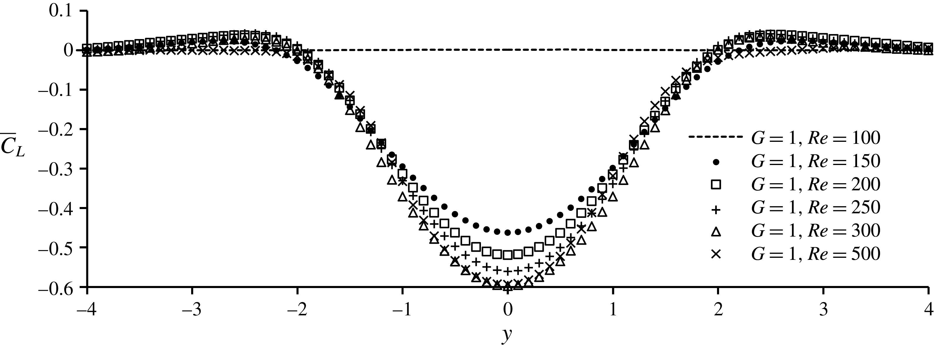
Figure 15 shows the variation of the mean sectional lift coefficient of the UC for all the cases with
 $G=1$
. The affected length of the lift coefficient of the UC by the asymmetry of the gap flow is approximately 4 diameters for all the cases in figure 15. The magnitude of the mean lift coefficient peaks at the centre of the UC and reduces to nearly zero at
 $y=\pm 4$
. The maximum mean lift coefficient at the centre of the UC is between 0.4 and 0.6 for
 $Re\in [150,500]$
. The maximum lift coefficient at the centre of the UC occurs at
 $Re=300$
.
Variation of the mean sectional lift coefficient of the UC for the cases with non-zero mean lift coefficient at the centre part of the UC.

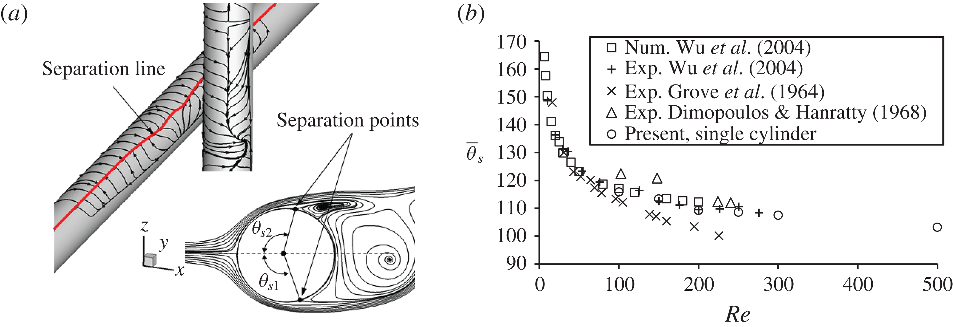
The DC has a significant effect on the separation point on the upstream cylinder. The separation point in a boundary layer is determined as the position on the cylinder wall where the shear stress is zero (Wu et al.
Reference Wu, Wen, Yen, Weng and Wang2004; Abrahamsen Prsic et al.
Reference Abrahamsen Prsic, Ong, Pettersen and Myrhaug2014). The separation angle, denoted as
 $\unicode[STIX]{x1D703}_{s}$
, is measured along the cylinder surface from the front stagnation point to the separation point, as shown in figure 16(a), where the streamlines calculated from the shear stress are plotted on the cylinder surfaces in the three-dimensional view and the streamlines in a cross-section is plotted in the two-dimensional view. Due to the existence of the DC, the positon of the separation point varies along the span of the UC. Connecting all the separation points along either the top or the bottom side of the UC forms a separation line. If the flow is symmetric the two separation angles
 $\unicode[STIX]{x1D703}_{s1}$
and
 $\unicode[STIX]{x1D703}_{s2}$
defined in figure 16(a) are the same. The separation angle oscillates with time if vortex shedding occurs. The mean separation angle (averaged over time) on the bottom and top sides of the UC are defined as
 $\bar{\unicode[STIX]{x1D703}}_{s1}$
and
 $\bar{\unicode[STIX]{x1D703}}_{s2}$
, respectively. Flow past an isolated single cylinder is simulated and the calculated mean separation angle of a single cylinder
 $\bar{\unicode[STIX]{x1D703}}_{s}$
as a function of the Reynolds number is compared with other published data (Grove et al.
Reference Grove, Shair, Petersen and Acrivos1964; Dimopoulos & Hanratty Reference Dimopoulos and Hanratty1968; Wu et al.
Reference Wu, Wen, Yen, Weng and Wang2004) in figure 16(b). The mean separation angle decreases with increasing Reynolds number in all of the studies, especially when the Reynolds number is small. The present numerical results of
 $\bar{\unicode[STIX]{x1D703}}_{s}$
agree well with the most recent experimental data by Wu et al. (Reference Wu, Wen, Yen, Weng and Wang2004).
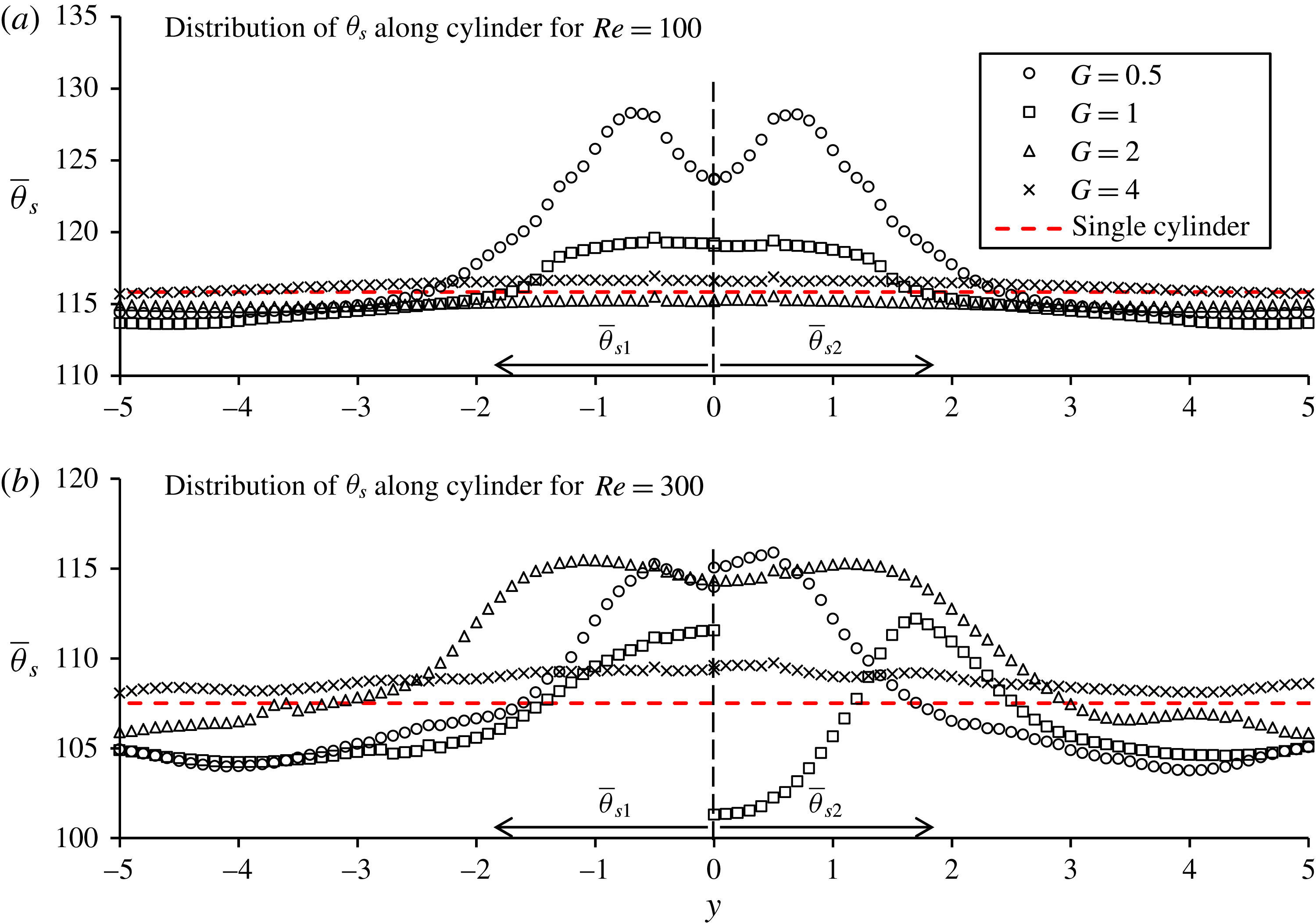
Figure 17(a,b) shows the variation of the separation angle along the UC for
 $Re=100$
and 300, respectively. Because the distribution of the separation angle is symmetric with respect to the
 $y=0$
point, the separation angles on the bottom and top sides of the UC (
 $\bar{\unicode[STIX]{x1D703}}_{s1}$
and
 $\bar{\unicode[STIX]{x1D703}}_{s2}$
) are presented on the
 $y<0$
and
 $y>0$
sides of figure 17, respectively. It has been seen in figure 16 that a reduction of Reynolds number leads to an increase in the separation angle. The separation angle near the centre of the UC is generally increased mainly because the blockage effect of the DC reduced the flow velocity at the side of the UC, resulting in a reduction of the effective Reynolds number locally. It can be clearly seen that the separation angle on the bottom side of the UC (
 $\bar{\unicode[STIX]{x1D703}}_{s1}$
) is very different from that on the top side (
 $\bar{\unicode[STIX]{x1D703}}_{s2}$
) at
 $G=1$
and
 $Re=300$
in figure 17(b). The wake flow behind the centre of the UC for
 $G=1$
and
 $Re=300$
is as asymmetric as that shown in figure 14(b). The asymmetric flow leads to separation angles on the bottom and top side of the centre of the UC greater and smaller than the separations angle of a single cylinder, respectively. When
 $G=1$
and
 $Re=100$
, both separation angles on the two sides of the centre UC are different from each other but they are both greater than that of a single cylinder.
(a) Definition of the separation line and separation points for
 $Re=100$
and
 $G=0.5$
; (b) variation of the angle of separation with the Reynolds number for a single cylinder.

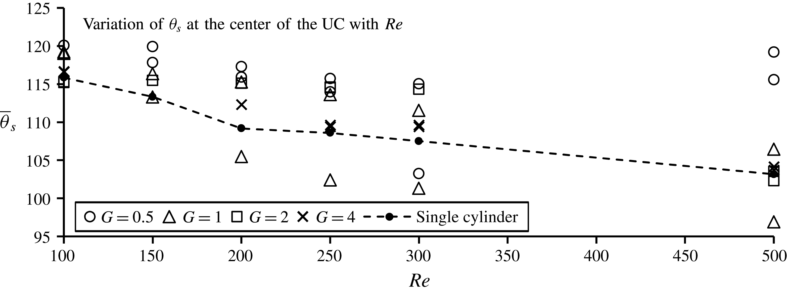
Figure 18 shows the variation of the separation angle at the centre of the UC with the Reynolds number for all the simulated gap ratios. The separation angles on both the bottom and top sides of the centre of the UC are plotted in figure 18. The cases with two separation angles in figure 18 are those cases where
 $\bar{\unicode[STIX]{x1D703}}_{s1}\neq \bar{\unicode[STIX]{x1D703}}_{s2}$
due to the asymmetry of the wake flow. It can be seen that the separation angle is greater than that of a single cylinder whenever the flow is symmetric (
 $\bar{\unicode[STIX]{x1D703}}_{s1}=\bar{\unicode[STIX]{x1D703}}_{s2}$
). One separation angle on one side (bottom or top) of the centre of the UC can be smaller than that of a single cylinder only when the flow is asymmetric with
 $\bar{\unicode[STIX]{x1D703}}_{s1}\neq \bar{\unicode[STIX]{x1D703}}_{s2}$
. Both the increase of the separation angle and the decrease of the local velocity at the centre of the UC due to the blockage effect of the DC lead to a significant reduction of the drag coefficient locally, which will be discussed in § 3.3.
Variation of the separation angle along the UC.

Variation of the separation angle at the centre of the UC with the Reynolds number.

3.3 Force coefficient
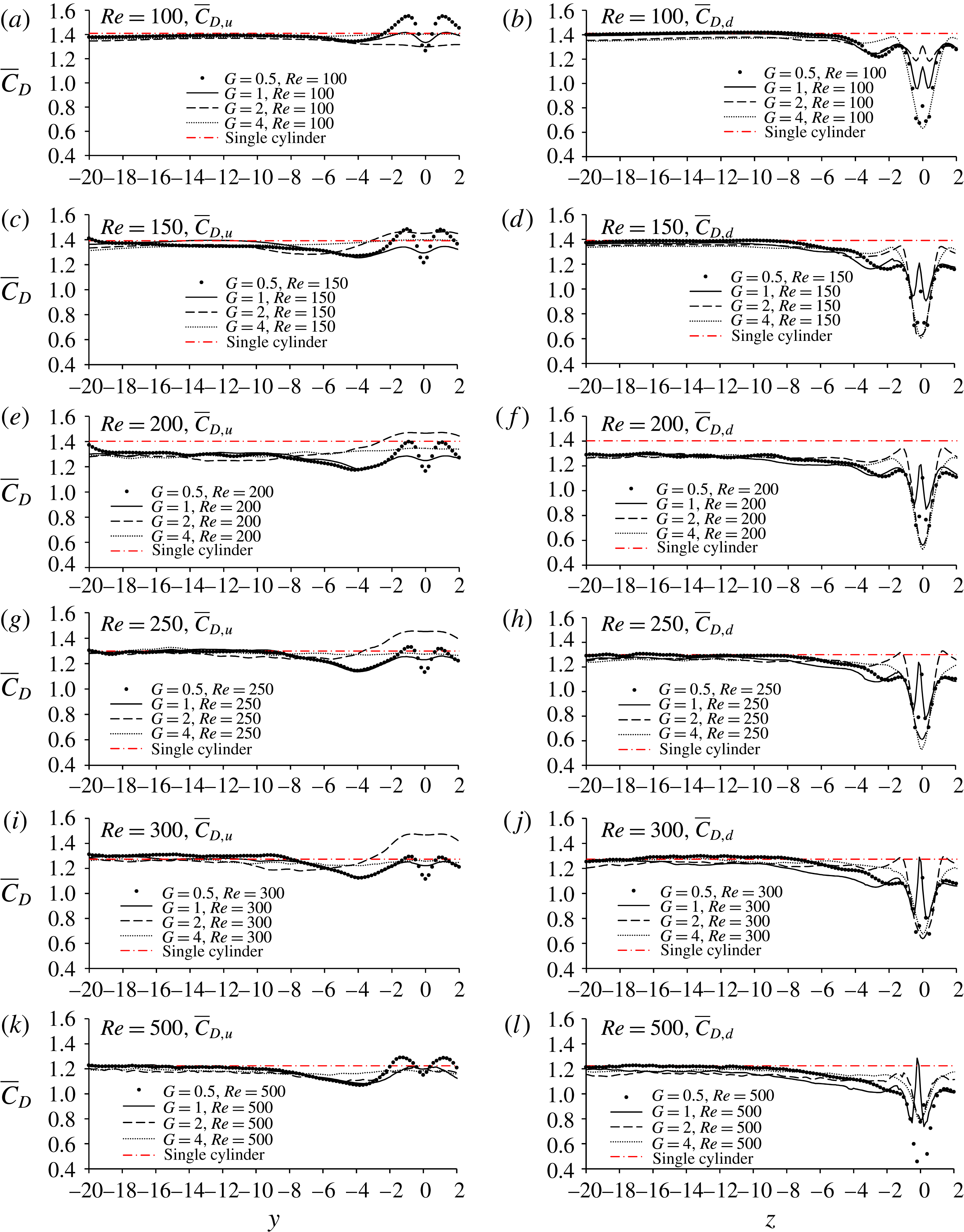
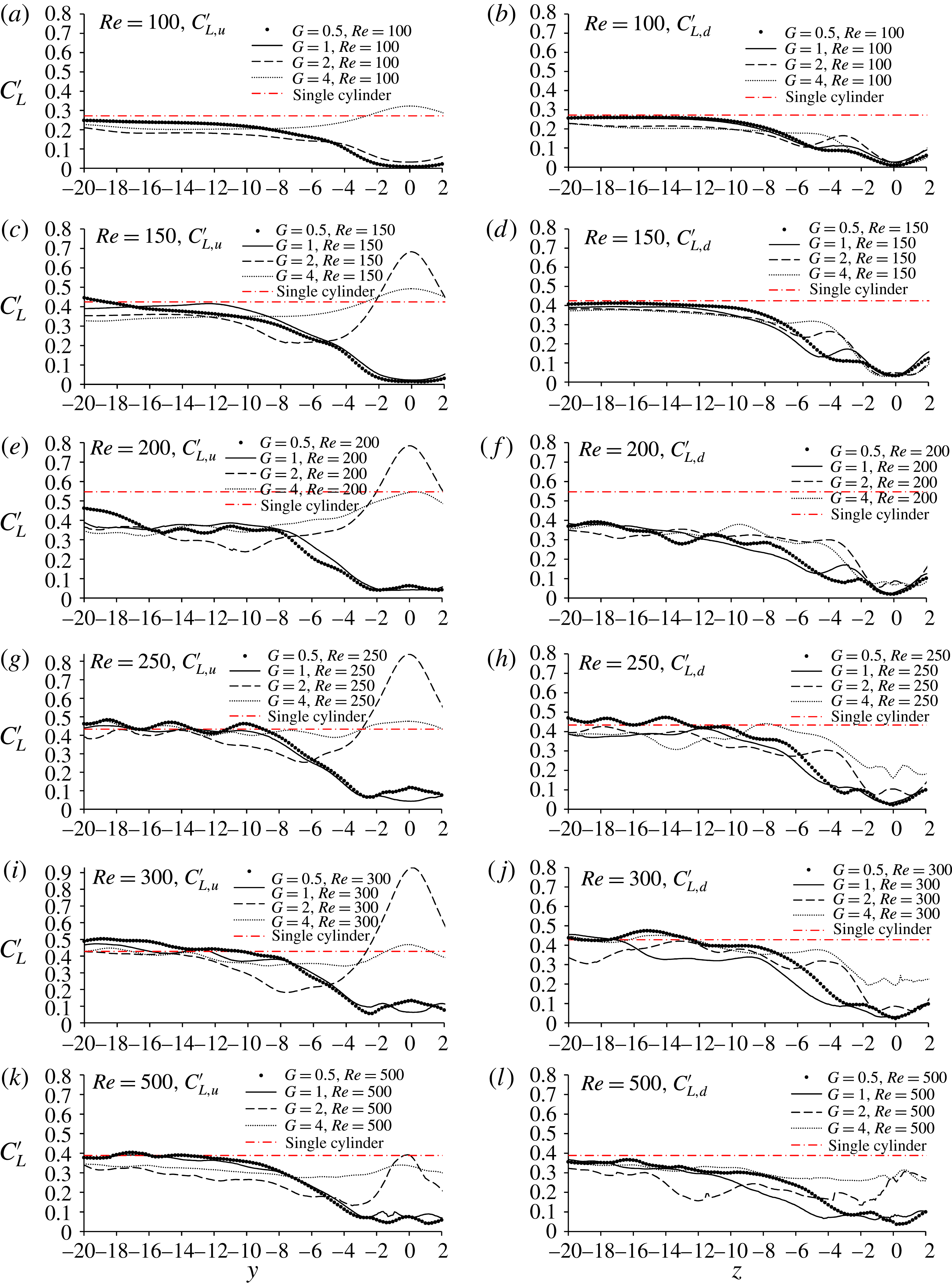
Figures 19 and 20 show the distributions of the mean drag coefficient and the standard deviation (SD) of the lift coefficient along half of the cylinder span, respectively. The prime and overbar on a variable represent the standard deviation and mean value, respectively. The subscripts ‘
 $d$
’ and ‘
 $u$
’ are used to denote the downstream and upstream cylinders, respectively. The distribution of the force coefficient on half of each cylinder is presented because the statistical values of the force coefficients on one half are almost the same as those on the other half. The corresponding force coefficients of an isolated cylinder are also shown in the figures for comparison. The effect length of the gap on the mean drag coefficient on both cylinders is approximately 8 from the cylinder centres. The mean drag coefficient of the centre of the DC significantly decreases compared with that of a single cylinder.
Distribution of the sectional force coefficient along half of the cylinder span.

Distribution of the standard deviation of the lift coefficient along half of the cylinder span.

From figure 20 it can be seen that the interference between the two cylinders affects the lift coefficient for at least 12-diameter long cylinder spans from the cylinder centre, which justifies the necessity of using an at least 24-diameter wide computational domain in the numerical simulations. It appears that the influence length of the gap on the mean drag coefficient is slightly shorter than that on the SD lift coefficient. The mean drag coefficient and the standard deviation of the lift coefficient near the ends of the cylinders are very close to those of an isolated cylinder except when
 $Re=200$
, i.e. the critical Reynolds number between the 3-D and 2-D wake flows. The difference between the force coefficient at
 $Re=200$
of the two cylinders and that of an isolated cylinder can be explained by the flow transition. After the wake transits to three dimensions, the lift coefficient reduces significantly because the energy of the spanwise vortices transfers to the energy of the streamwise vortices. When numerically simulating the flow past an isolated cylinder at
 $Re=200$
, the flow was found to be two-dimensional because there was not any end effects (Zhao et al.
Reference Zhao, Thapa, Cheng and Zhou2013). However, the strong centre effect of the two cylinders in cruciform arrangement makes the flow easily transit to three dimensions at
 $Re=200$
. The SD lift coefficient outside the central area of the cylinders is still significantly smaller than that of an isolated cylinder at the same
 $Re=200$
, which is mainly because the flow is three-dimensional in the present two cylinder system and two-dimensional for an isolated single cylinder.
When the gap ratio is
 $G=0.5$
,
 $\bar{C}_{D,u}$
reaches its minimum value at the centre of the upstream cylinder and has two maximum values near
 $y=\pm 1$
. To explain the variation of the mean drag coefficient near the middle span of the cylinder, the contours of the mean pressure coefficient on the cylinder surfaces are presented in figure 21, where the pressure coefficient is defined as
 $C_{p}=(p-p_{\infty })/(\unicode[STIX]{x1D70C}U^{2}/2)$
, with
 $p_{\infty }$
the pressure of the free stream and the position angles
 $\unicode[STIX]{x1D6FC}=0^{\circ }$
and
 $180^{\circ }$
represent the downstream and upstream edges of a cylinder, respectively. The occurrence of the minimum
 $\bar{C}_{D,u}$
at approximately
 $y=0$
can be explained by the pressure distribution and the vortex flow pattern. It can be seen from the vortex flow patterns in figure 14(a) that the flow in front of the DC converges towards the centre on the x–z plane and reverses. Without vortex shedding, the downstream point of UC is an stagnation point, where the pressure is locally high, resulting in a local reduction in
 $\bar{C}_{D,u}$
. A local increase in the pressure near
 $y=0$
and
 $\unicode[STIX]{x1D703}=0^{\circ }$
can be seen in the pressure contours in figure 21(a).
Generally,
 $\bar{C}_{D,d}$
is small near the centre of the downstream cylinder because of the shadowing effects of the UC. Whenever the vortex shedding from the centre of the upstream cylinder does not occur, the centre point of the front surface of the DC is also a stagnation point with high pressure (see
 $Re=100$
,
 $G=1$
in figures 14
b and 21
d), resulting in a local maximum value of
 $\bar{C}_{D,d}$
at
 $z=0$
.
Contours of the pressure coefficient along the cylinder surfaces.

The standard deviation of the lift coefficient is correlated to the unsteady vortex shedding. If vortex shedding from the centre of the upstream cylinder does not occur, the SD lift coefficient near the centre of the upstream cylinder is significantly smaller than that of an isolated cylinder. It is interesting to see that when
 $G=2$
, the SD lift coefficient at the centre of the UC is significantly greater than those near the two ends of the cylinder. The reason for the increase of
 $C_{L,u}^{\prime }$
at the centre of the upstream cylinder is due to the K mode vortex shedding mode. If the vortex shedding is in K mode, the vortex shedding from the centre of the UC is enhanced because the vortices from the UC converge towards the centre line as shown in figure 11(b,c). The convergence of the vortices towards the centre increases the strength of the vorticity behind the centre of the UC and consequently increases
 $C_{L,u}^{\prime }$
locally. In addition, the flow on the x–z plane also converges towards the centre of the front face of DC as shown in figure 14. This also enhances the vortices behind the centre of the DC and
 $C_{L,u}^{\prime }$
.
Once the vortex shedding from the DC centre occurs (as the result of increasing
 $G$
), the behaviour of
 $C_{L,d}^{\prime }$
is different from that of two parallel cylinders in a tandem arrangement. If two parallel cylinders are in tandem in a fluid flow with gap ratio slightly greater than the critical value for vortex shedding from the UC, the SD lift coefficient of the downstream cylinder increases significantly (Sumner Reference Sumner2010). In contrast to that in the case of two parallel cylinders, the SD lift coefficient at the centre of the DC is generally reduced compared with that of a single cylinder, even when the vortex shedding from the centre of the UC occurs. The reason why the SD lift coefficient at the centre of the downstream cylinder reduces significantly can be explained as follows. Firstly, the shear layers generated from the UC do not contribute to
 $C_{L,d}^{\prime }$
because their vorticity are perpendicular to the DC. Secondly, the shear layers from the two sides of the centre part of the DC are not likely to form strong vortices in the
 $z$
-direction because of their interaction with the vortices from the upstream cylinder. It can be seen in figure 7 that the vortices behind the middle of the DC are not aligned in the axial direction of the DC at
 $G=2$
and 4 and they are very weak. Thirdly, the shadowing effect of the UC reduces the fluid velocity that approaches the DC.
Near the two ends of each cylinder, the SD lift coefficient for
 $G=2$
and 4 is found to be slightly smaller than that of a single cylinder. The slight reduction of the lift coefficient is mainly because of the inclination of the wake vortices in the K mode vortex shedding. The oscillation of the lift coefficient is mainly the result of the vortices developed in the axial direction of a cylinder. If the wake vortices are inclined, their component in the axial direction becomes weak, leading to a reduction in the lift coefficient. The degree of the inclination of the wake vortices in the K mode vortex shedding is correlated with the reduction the lift coefficient. The largest inclination of the vortices at
 $G=2$
corresponds to the most significant reduction in the lift coefficient.
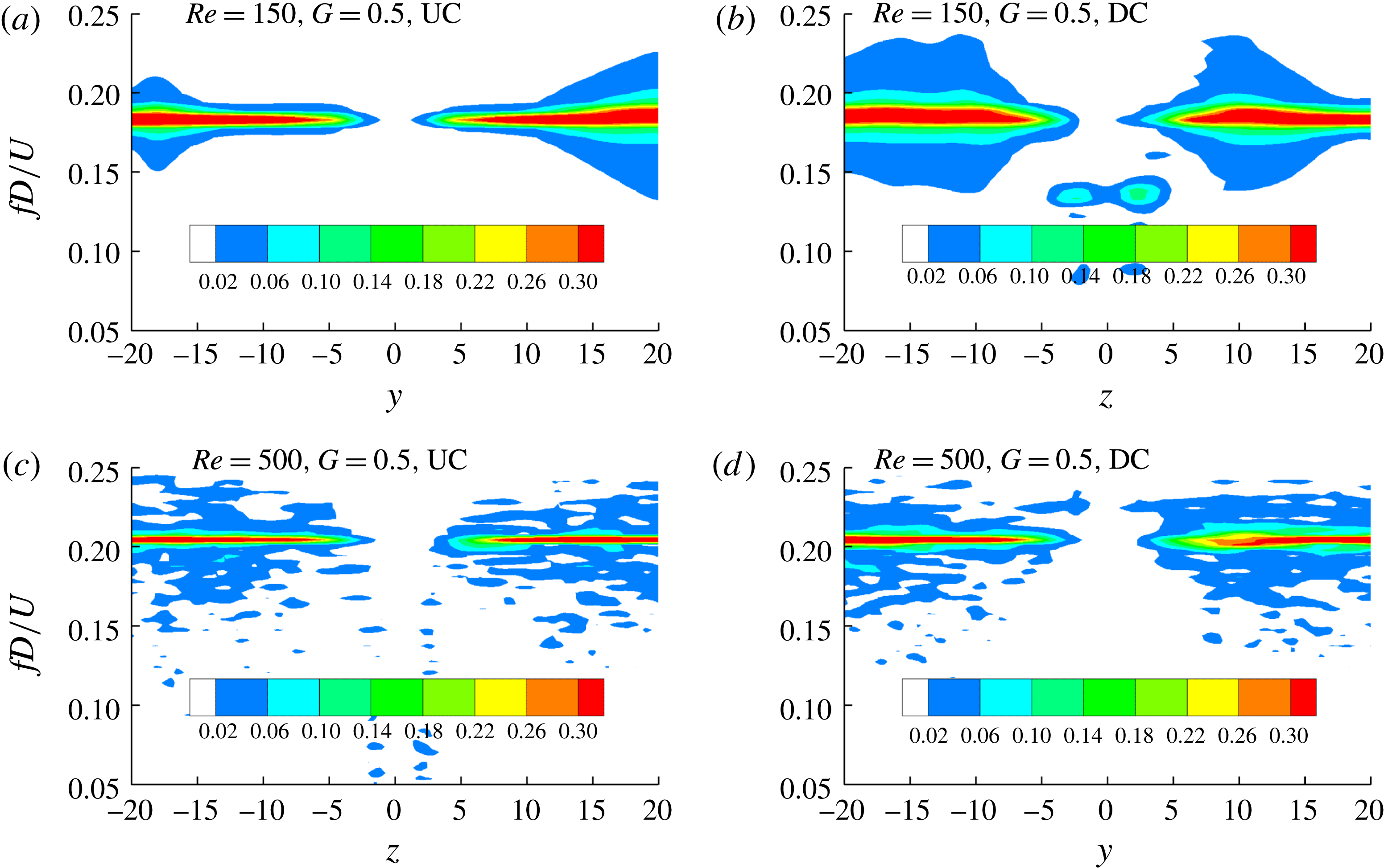
The vortex shedding frequency is the same as the frequency of the lift fluctuation for a circular cylinder in steady flow. The frequency of the sectional lift coefficient for each of the two crossing cylinders is found to remain unchanged along the cylinder span. This can be evidenced by the contour of the lift coefficient amplitude on the length–frequency plane shown in figure 22. To produce figure 22, a fast Fourier transform (FFT) of the sectional lift coefficient at all the sections with an interval of 0.2 along the cylinder span is conducted. It can be seen in figure 22 that the frequency varies little along the cylinder span except at the centre part of DC at
 $Re=150$
and
 $G=0.5$
, where the lift coefficient is extremely small. The decrease in the lift coefficient is due to the disconnection of the lift coefficient contours shown in figure 8.
Contour of the amplitude of
 $C_{L}$
on the
 $z$
–
 $f$
plane based on FFT transform.

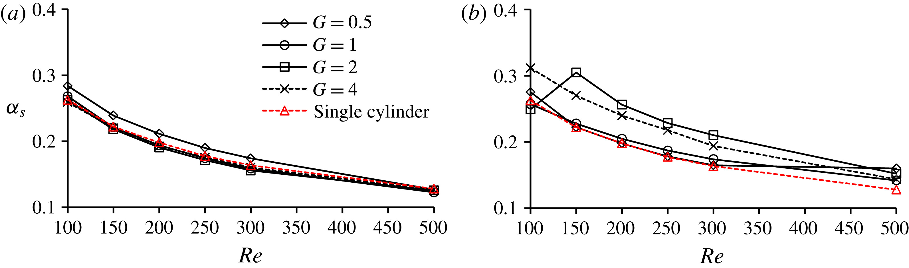
The contribution of the drag force due to the shear stress to the total drag force is evaluated by the ratio of the drag force due to the shear stress to the total drag force on the cylinders, which is denoted as
 $\unicode[STIX]{x1D6FC}_{s}=\bar{C}_{D,shear}/\bar{C}_{D}$
, where
 $\bar{C}_{D,shear}$
is the component of the mean drag coefficient due to shear stress. Figure 23 shows the variation of the coefficient
 $\unicode[STIX]{x1D6FC}_{s}$
at the centres of the UC and DC with the Reynolds number for all the simulated gap ratios. It can be seen in figure 23(a) that
 $\unicode[STIX]{x1D6FC}_{s}$
at the centre of the UC is very close to that of a single cylinder except when
 $G=0.5$
. The variation of
 $\unicode[STIX]{x1D6FC}_{s}$
of the DC with the Reynolds number is found to be correlated with the gap flow mode listed in table 1. Whenever the gap flow is in TV or NV mode, the contribution of the shear drag coefficient increases, i.e.
 $\unicode[STIX]{x1D6FC}_{s}$
increases significantly. Once vortex shedding in the gap is in the SG mode, i.e. the vortex shedding from the centre of the UC occurs,
 $\unicode[STIX]{x1D6FC}_{s}$
at the centre of the DC is very close to that of a single cylinder. The increase in
 $\unicode[STIX]{x1D6FC}_{s}$
of the DC in the TV and NV gap flow mode is mainly because of the decrease in the pressure drag coefficient. In the TV and NV mode, the low pressure in the gap caused by the vortex behind the UC leads to a small drag force of the DC. This makes the weight of the friction drag coefficient of the DC increase, i.e.
 $\unicode[STIX]{x1D6FC}_{s}$
increase.
Variation of the shear to total drag force ratio (
 $\unicode[STIX]{x1D6FC}_{s}$
) at the centres of the UC and DC with the Reynolds number.

4 Conclusions
Numerical simulations of fluid flow past two circular cylinders in cruciform arrangement are conducted for gap ratios of
 $G=0.5$
, 1, 2 and 4 and Reynolds numbers between 150 and 500 with an interval of 50. The effects of the gap ratio between the two cylinders on the vortex shedding pattern and the force coefficients are analysed. Both the local flow pattern near the gap and the global flow pattern in the wake of the two cylinders are discussed. The conclusions are summarized as follows.
(i) The flow pattern near the gap can be classified into three categories: TV, NV and SG, depending on the Reynolds number and the gap ratio. The boundaries of the gap ratio between TV and NV and that between NV and SG decrease with the increase of the Reynolds number.
(ii) The global vortex shedding in the wake of the two cylinders can be classified into two modes: K mode and P mode. K mode occurs in two scenarios. (a) The gap is slightly greater than the boundary gap ratio between NV and SG, i.e.
 $G=2$
; (b) If the Reynolds number is very small, the K mode can occur when the gap flow is in the SG pattern. Asymmetric wake flow behind the centre of the UC develops when the gap is slightly smaller than the critical value between NV and SG, resulting in non-zero sectional lift coefficients near the centre of the UC.
(iii) The flow pattern affects the force coefficient significantly. If local flow near the gap is in the TV or NV pattern, maximum values of
$\bar{C}_{D,u}$
and
$\bar{C}_{D,d}$
are found at the centres of the UC and DC, respectively.
$C_{L,u}^{\prime }$
at the centre of the UC is greater than that of an isolated cylinder if the gap ratio is slightly greater than the critical value between NV and SG. This is because of the convergence of the vortices towards the centre in the K mode.
$C_{L,u}^{\prime }$
is smaller than that of a single cylinder if the flow near the gap is TV or NV because there is no vortex shedding from the centre of the UC.
$C_{L,d}^{\prime }$
near the centre of the DC is smaller than that of an isolated cylinder, mainly because of the shadowing effect from the UC.(iv) The force coefficients of both cylinders at
$Re=200$
are significantly smaller than that of an isolated cylinder, because
$Re=200$
is the critical Reynolds number for the flow transitioning from two to three dimensions. In the numerical simulation at
$Re=200$
, the flow in the wake of an isolated cylinder is two-dimensional because there is no end effect and the flow in the wake of two circular cylinders in a cruciform arrangement is three-dimensional because of strong effect from the gap.(v) The gap affects the force coefficients on 24 diameter long span of each cylinder, making it necessary to choose at least 24 diameter long cylinders for simulating flow past two cylinders in a cruciform arrangement.


Acknowledgements
The authors would like to acknowledge the support from the National Natural Science Foundation of China (NSFC), grant numbers 51628901 and 51490673; and the support from the National Key R&D Program of China, grant number 2016YFE0200100.