Statement Of The Problem

In duration modeling, monotone likelihood occurs when ‘at each failure time, the covariate value of the failed individual is the largest of all covariate values in the risk set at that time or when it is always the smallest’ (Heinze and Schemper Reference Heinze and Schemper2001, 144; also see Tsiatis Reference Tsiatis1981). Put differently, monotone likelihood is a property of samples where covariate values are monotonic when ordered according to failure time. Table 1 provides a stylized example. Here, X ₁ and X ₂ are monotonic continuous covariates: they take on values that are always the largest (X ₂) or always the smallest (X ₁) of all covariate values in the risk sets R(t _f) = {t ₁, t ₂, t ₃, t ₄, t ₅}.Footnote ¹ X ₃ provides another example of monotonicity, this time in a binary predictor variable, where the values X ₃ = 1 for the failed individuals at R(t _f) = t ₁, t ₂, t ₃ are the largest values of X ₃ in the ordered risk set. X ₄ and X ₅ then represent non-monotonic ordering of failure times for continuous and binary covariates, respectively.

Table 1.

Monotonicity in continuous and dichotomous predictors

Because the predictors X ₁, X ₂ and X ₃ are monotonic, the (partial) likelihood of one's estimated duration model will be monotone for the coefficient estimates associated with these predictors. Consequently, while the likelihood function will converge to a finite value, estimates of ${{\beta _1}}$, ${{\beta _2}}$, and ${{\beta _3}}$ will diverge to positive or negative infinity. For an estimator that does not account for this sample property, the net result will be biased, model-dependent estimates with arbitrarily large (or small) parameter values.Footnote ²

In practice, monotone likelihood most often occurs when a value of a covariate, or a linear combination of covariates, uniquely correspond(s) to all termination events – a phenomenon akin to ‘separation’ in other binary response models. In their pioneering work on this issue, Albert and Anderson (Reference Albert and Anderson1984) distinguish between two types of separation: ‘complete’ and ‘quasi-complete’.Footnote ³ Translated into a duration modeling framework, complete separation refers to instances in which the values of one or more covariates uniquely correspond to all termination and survival events;Footnote ⁴ quasi-complete separation refers to instances in which one value of a covariate uniquely corresponds to all termination events, but not to all survival events.Footnote ⁵ In either case, monotone likelihood arises due to the absence of overlap of failure times between two or more groups. To see this intuitively, consider the case of a quasi-completely separating dichotomous predictor X _D, where all values X _D = 0 correspond to the full set of termination events. In such cases, there is no overlap of failure times in the two groups X _D = 0 and X _D = 1, as there are no termination events associated with the value X _D = 1. Were a researcher to order X _D's values according to failure time, the resulting vector would be monotonic (in this case, never increasing, as X _D never varies from 0 when a termination event occurs).

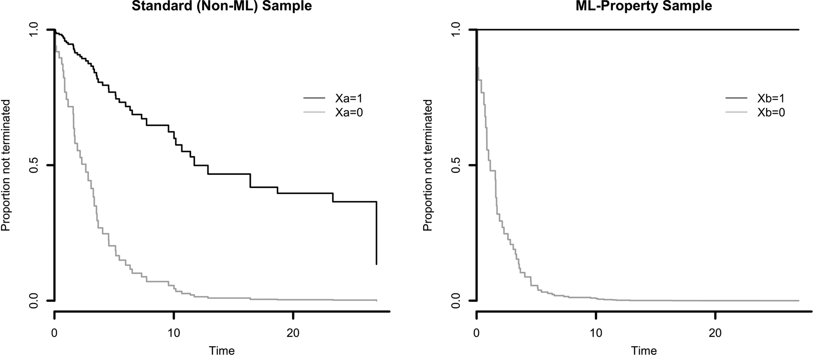
Figure 1 provides a visual representation of the problem using simulated duration data. In the left panel, we plot predicted survival curves from a Cox model that incorporates a single dichotomous covariate, X _a, that is non-monotonic (that is, there is overlap of failure times in the groups X _a = 1 and X _a = 0). In this panel, the predicted proportion of cases that have not yet terminated gradually declines as a function of X _a and time. In the right panel, we plot predicted survival curves from a Cox model that incorporates a single dichotomous covariate, X _b, that is quasi-completely separating (and thus, monotonic). In this case, all X _b = 0 correspond to the full set of termination events, meaning that there are no termination events associated with the value X _b = 1, and thus there is no overlap of failure times in the two groups X _b = 0 and X _b = 1. This causes the survival curve for X _b = 1 to become horizontal in orientation. The corresponding Cox model estimate for X _b will diverge to negative infinity.

Figure 1.

Survival curves for simulated Cox regressions

Importantly, the absence of a quasi-completely separating covariate does not eliminate the risk of monotone likelihood, for two reasons. First, covariates do not need to be quasi-completely separating to be monotonic when ordered according to failure time. Secondly, even when no single covariate is monotonic, a linear combination of covariates can be. As above, this leads to a flattening of the likelihood function and an inflation of parameter values towards infinity.

At its root, then, monotone likelihood is the result of highly imbalanced and thus highly predictive covariates. This problem can be decomposed into a number of contributing factors (Bryson and Johnson Reference Bryson and Johnson1981; Heinze and Schemper Reference Heinze and Schemper2001; Johnson et al. Reference Johnson1982; Loughin Reference Loughin1998):

• • Dichotomous predictors. Models that rely on a large number of dichotomous predictors are more likely to be afflicted by monotone likelihood. The categorical nature of these variables restricts their range to just two values, thereby rendering monotonicity more likely. While monotone likelihood may occur with any type of data, it is less common in the case of continuous independent variables.

• • Number of covariates. As the number of included covariates increases, the probability that the likelihood function will be monotone in at least one of the regression parameters increases for two reasons. First, there are more opportunities for at least one covariate to be monotonic when ordered according to failure time. Secondly, even where no single covariate is monotone, a function of the covariates can be.

• • Small sample sizes. As sample size decreases, the probability that at least one covariate is monotonic when ordered according to failure time increases as a function of small sample bias.

• • Proportion of censored observations. Increased censoring generates imbalance by increasing the number of zeros (censored observations) to ones (terminations) on the termination indicator variable. Datasets that incorporate time-varying variables are especially susceptible to this concern owing to their counting process data structure, which breaks up individual cases into multiple observation periods.

The various statistical programs and packages commonly used in the political science literature differ in how they deal with monotone likelihood. Some packages will detect nonconvergence, warn the user and fail to estimate parameter values;Footnote ⁶ others will detect nonconvergence and issue a warning, yet will still estimate parameter values even for those variables afflicted by monotone likelihood;Footnote ⁷ and still others will fail to detect nonconvergence and estimate all parameter values in the model.Footnote ⁸ The parameter estimates returned in these instances will typically correspond to the set of extreme, but finite, values for which changes in a model's log-likelihood fall below a given tolerance threshold, which itself is variable across software and estimation routines.Footnote ⁹ Consequently, in cases of monotone likelihood, a researcher's results will vary as a function of the software program and packages employed.

Faced with estimates that imply fitted probabilities that converge to extreme positive or negative values, researchers are often forced to choose among a range of distasteful remedies. Heinze and Schemper (Reference Heinze and Schemper2001, 114–115), for instance, review some of these issues. First, some researchers simply drop the offending variable from their analysis, introducing omitted variable bias. Secondly, researchers may choose to change their modeling strategy, risking model misspecification in light of censored or truncated data. Thirdly, researchers may stratify on the offending variable, allowing the hazard to vary by each category of the problematic variable, but consequently forgoing estimating its own effect on duration. Fourthly, biased estimates can result in misinterpretation of substantive effects, or indeed in a decision to avoid interpreting the results altogether. Fifthly, and perhaps most insidious of all, a failure to understand the underlying causes of monotone likelihood can contribute to the file drawer problem, where researchers simply do not publish or report models that seem otherwise incorrect, hard to understand, or that fail to support a theory's proposed hypotheses.

Notwithstanding these distasteful remedies, monotone likelihood remains a common problem in political science research. To evaluate the extent to which it affects the existing literature, we conducted a survey of all articles that employed a duration model between the years 2008–2018 and that appeared in one of three leading political science journals: the American Political Science Review, the American Journal of Political Science and the Journal of Politics.Footnote ¹⁰ Of the fifty-seven articles we identified, 14 per cent contained strong evidence of monotone likelihood. This represents a substantial share of contemporary duration model research across three of the discipline's top journals over the past decade. What is more, we found that monotone likelihood can be identified across the empirical subfields of political science – from American politics to comparative politics to international relations – and affects cross-national studies and subnational analyses alike. And importantly, this estimate is likely a conservative one in light of the file drawer problem noted above, whereby many studies afflicted by monotone likelihood are never published. Thus, our survey suggests that monotone likelihood regularly confronts researchers employing duration models in their empirical research. In what follows, we introduce a corrective for this methodological challenge and illustrate its advantages using a combination of mathematical exposition, Monte Carlo simulations and empirical applications.

A SOLUTION TO MONOTONE LIKELIHOOD

In recent years correctives have been developed for monotone likelihood – namely, the application of penalized maximum-likelihood estimation approaches to Cox regression models. In particular, a procedure developed by Firth (Reference Firth1993) to reduce the bias of maximum-likelihood estimates under monotone-likelihood conditions has been shown to solve the problem in a range of Cox regression applications (Heinze and Dunkler Reference Heinze and Dunkler2008; Heinze and Schemper Reference Heinze and Schemper2001), as well as for estimators designed for other limited dependent variables (Cook, Niehaus and Zuhlke Reference Cook, Niehaus and Zuhlke2018; Rainey Reference Rainey2016; Zorn Reference Zorn2005). With the application of penalized maximum-likelihood estimation, finite parameter estimates of constant and time-dependent effects can be obtained even in the presence of monotone likelihood.

In formal terms, monotone likelihood can generate bias in any estimated parameters (denoted generally as $\hskip3pt{\hat {\hskip-3pt\theta} }\hskip.5pt$) when the score function at the true $\hskip3pt{\hat {\hskip-3pt\theta} }\hskip.5pt$ is unbiased (that is, E[U(θ)] = 0) but its curvature is not linear in θ (that is, the rate of change of the function U(θ)^′′ ≠ 0). Given that E[U(θ)] = 0, any corresponding duration model's estimation functionFootnote ¹¹ that is linear in θ will converge to a finite value; this is precisely what the researcher wants when estimating a (generalized) linear model. However, because the function's curvature is not linear in θ, some parameter values will be severely biased upward (if U(θ)^′′ > 0) or downward (if U(θ)^′′ < 0).

Consequently, when estimating θ under conditions of monotone likelihood, the researcher introduces positive or negative bias into the score function. This arises even if the function is otherwise unbiased with respect to identification. And notably, because the rate of change of the score function's curvature is itself not linear, such bias will be increasing to infinity. This, in turn, can lead to at least one parameter estimate converging to −∞/ + ∞ and a model that arbitrarily over- or under-estimates the true covariate effects (Firth Reference Firth1993, 28; Heinze and Schemper Reference Heinze and Schemper2001, 114).

To ameliorate the impact of monotone likelihood in affected samples, one can introduce suitable corrective bias into the biased (partial) likelihood estimate $\hskip3pt{\hat {\hskip-3pt\theta} }\hskip.5pt$ (Firth Reference Firth1993). In contrast to other plausible correctives – such as removing the offending variable or arbitrarily trimming down the coefficient size – this approach involves using the function's (that is, U(θ)) own estimates to identify an informed correction that is proportional to the size of the uncorrected estimator's bias under monotone-likelihood conditions. Mathematically, this correction is expressed as follows. First, assume a standard Cox partial log-likelihood function:

(1)$$\ln L( \beta ) = \sum\limits_{i = 1}^m {\left\{{X_i\beta -\ln \left[{\sum\limits_{h\in R_j} {\exp ( X_h\beta ) } } \right]} \right\}} $$

where R _j denotes all observations at risk at time t _j, i denotes the N distinct event times, X_i denotes the covariates for observations that experienced a termination event at t _j, X_h denotes the covariates for all observations at risk, and β encompasses the associated coefficients (see Box-Steffensmeier and Jones Reference Box-Steffensmeier and Jones2004, 52). Now, recall that under monotone-likelihood conditions, our partial-likelihood estimate $\hskip3pt{\hat {\hskip-3pt\theta} }\hskip.5pt$ – or more specifically, our β parameters for the offending variable(s) therein, which we denote as β _r – is biased. The purpose of the corrective bias approach is to provide an informed correction that is proportional to the size of the bias in the estimator caused under monotone-likelihood conditions. Following Firth (Reference Firth1993), we term the new corrective function U(β _r)*, and express it as:

(2)$$U( {\beta_r} ) {\hbox{\ast}}{\equiv} U( {\beta_r} ) + \alpha _r = 0$$

where U(β _r) is the uncorrected partial likelihood-estimated covariate, and α _r is:

(3)$$\alpha _r = 0.5\ {trace}\left\{{{\bf I}{( \beta ) }^{{-}1}\left[{\displaystyle{{\partial {\bf I}( \beta ) } \over {\partial \beta_r}}} \right]} \right\}$$

In Equation 3, ${\bf I}( \beta ) ^{{-}1}$ is the inverse information matrix evaluated at each β, or the variance–covariance matrix for $\hat{\beta }$. The term in brackets [ ⋅ ] is the derivative of the information matrix with respect to β _r: (∂/∂β _r){0.5 log|i(β)|}. Accordingly, α _r can be estimated using the Newton–Raphson algorithm or other standard (partial) likelihood optimization routines, where each step is based on the current value of $\hat{\beta }$.Footnote ¹² In simple terms, this correction ‘pushes against’ the original (uncorrected estimator) bias. Thus, if U(β _r) has a positive bias, the score function will be shifted downward by α _r at each point; if U(β _r) has a negative bias, the score function will be shifted upward.

Modification of the score function in this manner directly addresses the aforementioned challenge of arbitrarily large (or small) parameter values in monotone-likelihood contexts through its assurance of finite parameter estimates (Heinze and Schemper Reference Heinze and Schemper2001, 115). To see the latter point, note that because this informed correction builds on the uncorrected function's own variance–covariance matrix, it is proportional to the size of the bias in the uncorrected estimator. This quality provides an important advantage over uninformed corrections, which are likely to over- or under-estimate the bias in the estimation results under monotone-likelihood conditions. Specifically, as β _r → ±∞, the highest/lowest observed value of a covariate x _k in each risk set gets weighted more heavily compared with other covariates, as long as there are at least k distinct failure times. This helps to ensure that even if the (log) likelihood L is monotone, the determinant of ${\bf I}( \beta ) $ still approaches zero, which in turn means that the penalized maximum likelihood L* is guaranteed to attain a finite, bias-corrected value of $\hskip3pt{\hat {\hskip-3pt\beta} }\hskip.5pt$. Indeed, as first illustrated by Firth (Reference Firth1993) in a general context and by Heinze and Schemper (Reference Heinze and Schemper2001) in a duration model context, L* is asymptotically consistent and is otherwise resistant to the small-sample biases and arbitrary parameter estimates that arise in (partial) likelihood estimation. In that regard, Firth's (Reference Firth1993) correction lowers estimation bias empirically, regardless of issues of substance (for example, ‘what is an intervention?’) or thresholds of ‘plausibility/implausibility’, which are inherently subjective to a particular application.

For the remainder of this article, we accordingly assess the benefits of penalized maximum likelihood in Cox regression applications – hereafter referred to as the ‘Firth Cox’ (Heinze and Dunkler Reference Heinze and Dunkler2008; Heinze and Schemper Reference Heinze and Schemper2001). The Cox model is generally viewed as the default choice among contemporary political scientists for applied duration modeling (Box-Steffensmeier and Jones Reference Box-Steffensmeier and Jones2004; Ruhe Reference Ruhe2018, 91), and can be reformulated and interpreted as an exponential family model (Heinze and Schemper Reference Heinze and Schemper2001; McCullagh and Nelder Reference McCullagh and Nelder1989, 429). The latter is appealing in this case in that it ensures that the bias-reducing properties of the Firth correction – as originally established for generalized linear models (Firth Reference Firth1993) – will carry over to the Cox context (Heinze and Schemper Reference Heinze and Schemper2001, 115). This property has been empirically confirmed for the Firth Cox model by both Heinze and Schemper (Reference Heinze and Schemper2001, 117) and Heinze and Dunkler (Reference Heinze and Dunkler2008, 6464), and thus serves as an additional justification for using the Firth Cox model in these contexts.

That being said, we note that monotone-likelihood issues can equally impact parametric duration models, such as the Weibull. Accordingly, in the ensuing sections we report empirical models based not only upon the standard Cox model and the Firth Cox model, but also upon the Weibull model. The latter application illustrates that the biases in non-corrected estimators under conditions of monotone likelihood in duration analysis are relevant to parametric and semi-parametric models alike.

Monte Carlo Simulations

To evaluate the causes of monotone likelihood – and to assess the potential for penalized maximum-likelihood estimation to address monotone-likelihood issues – we conducted a large number of Monte Carlo (MC) experiments. These experiments compare the performance of a standard Cox proportional hazard model to that of a Cox proportional hazard model with Firth's penalized maximum-likelihood correction (Firth Cox). We expand upon and improve past simulation studies of monotone likelihood in three ways.

First, we examine the problem under a wider range of conditions: five varying levels of censoring,Footnote ¹³ at six different sample sizes,Footnote ¹⁴ across three different specification scenarios.Footnote ¹⁵ Importantly, our MC experiments are designed to ensure we do not directly modify the severity of monotone likelihood, but rather allow the severity of this problem to arise organically as a function of (imbalanced) independent variables that are themselves a product of varying sample sizes, changing levels of censoring and different rates of omitted variables.

Secondly, unlike previous studies, we simulate duration data to match the (nonparametric) Cox model's assumed data-generating process via the methods recently developed by Harden and Kropko (Reference Harden and Kropko2019), including a mixture of continuous and imbalanced binary predictors.

Finally, we assess the performance of the Cox and Firth Cox models across our resulting ninety distinct combinations of varying conditions in terms of (1) the proportion of relevant simulations that saw nonconvergence due to infinite or near-infinite parameter estimates and (2) our parameter estimates' root mean squared errors (RMSEs), averaged across all simulations. When doing so, we maintain consistent iteration limits on the Cox and Firth Cox models during each simulation run, which provides us with conservative estimates of the latter model's abilities to overcome monotone-likelihood issues. Together, these MC experiments provide to our knowledge the most comprehensive assessment of the performance of Firth's correction to duration modeling to date.

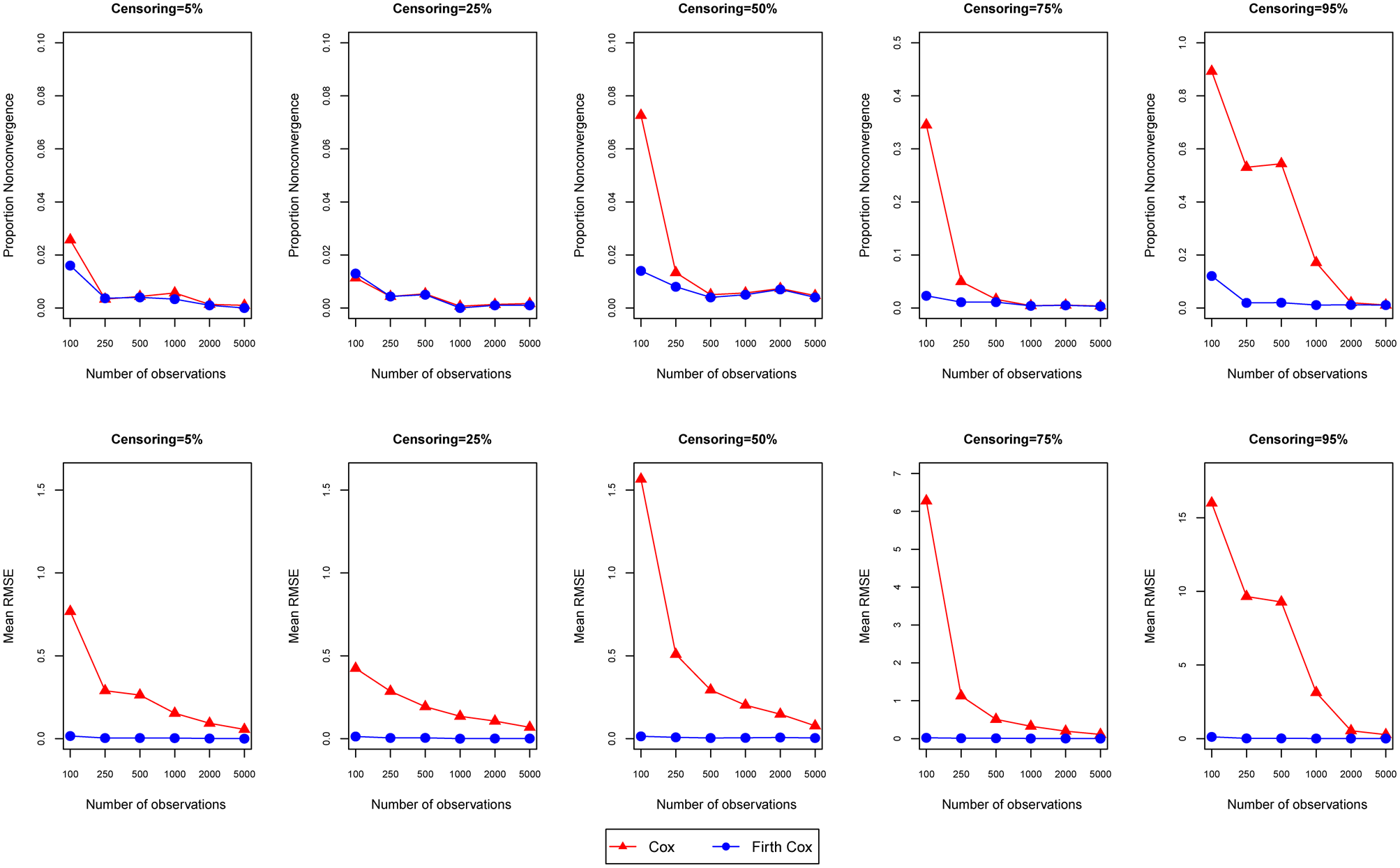
Figure 2 summarizes the results of our MC experiments, reporting nonconvergence rates and RMSEs for the estimates associated with a simulated binary independent variable of interest, X ₁.Footnote ¹⁶ Each column of subfigures depicts a different level of censoring; the x-axes vary the N evaluated; and the y-axes depict either the proportion of nonconvergence obtained across all relevant simulations (subfigure row 1) or the RMSEs for $\widehat{{\beta _1}}$ (subfigure row 2). We plot the relevant values obtained for our Cox (triangles) and Firth Cox (circles) models within each subfigure after averaging over the distinct levels of omitted variable bias evaluated. The latter condition was collapsed in Figure 2 for summary purposes; it is presented in disaggregated fashion in the Appendix. Note that the scale of nonconvergence and RMSEs across these different specifications increases markedly as the level of censoring increases, as denoted by the differing y-axis values on these plots.

Figure 2.

Nonconvergence and RMSEs for X ₁ across all Monte Carlo experiments

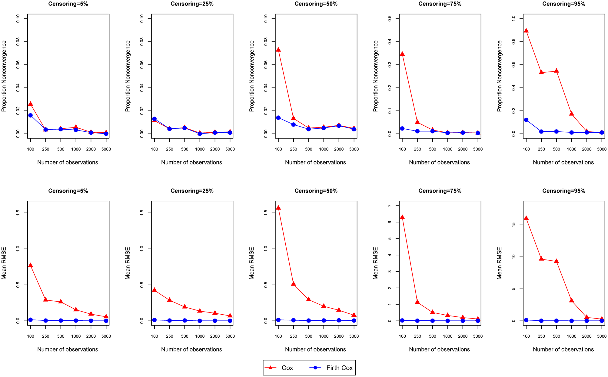
We find that analyses afflicted by monotone likelihood will frequently encounter nonconvergence and inaccurate parameter estimates when using a standard Cox model, but not when using the Firth Cox model. This is especially the case for samples of 100–500 observations, regardless of the level of censoring. However, for levels of censoring at or greater than 75 per cent – common in duration model applications with time-varying covariates – the aforementioned threats to accuracy and convergence with the standard Cox model increase substantially, and can persist in samples as large as 1,000–2,000 observations. For instance, Figure 2's subfigure columns 4 and 5 (75–95 per cent censoring) demonstrate that, using samples of 100–500 observations, researchers will on average encounter nonconvergence rates of 40 per cent for the standard Cox model, compared to nonconvergence rates of 3 per cent for the Firth Cox model. Under these same conditions, the Cox model $\widehat{{\beta _1}}$ RMSEs are on average 250 times larger than those obtained using the Firth Cox model. At samples of 1,000–2,000 and 95 per cent censoring, the Firth Cox model continues to recover $\widehat{{\beta _1}}$s that are 165 times more accurate than those of the Cox model, with nonconvergence rates that are 8.4 percentage points lower than the Cox model. Our additional MC assessments (reported in the Appendix) reaffirm each of these findings.

In short, monotone likelihood arising from imbalanced predictors leads to inaccuracy and nonconvergence in parameter estimates for the Cox model when the number of observations is lower than 1,000. At levels of 75–95 per cent censoring, the Cox model becomes practically unusable for small-to-moderate sample sizes, exhibiting nonconvergence due to (near-)infinite parameter estimates in a substantial share of all such simulations. By contrast, the Firth Cox model is much less sensitive to these monotone-likelihood challenges, and in most instances recovers parameter estimates that are several orders of magnitude more accurate than those of the Cox model. Indeed, even in those cases where the Cox and Firth Cox models exhibit similar nonconvergence rates, we find that the latter always obtain lower RMSEs across all parameters and experimental conditions evaluated, and further confirm these findings for mean squared errors in the Appendix. In line with recent logit-based findings (Rainey and McKaskey Reference Rainey and McKaskeyForthcoming), these results suggest that penalized maximum-likelihood corrections may be preferable to standard Cox estimation frameworks in regards to the accuracy of parameter estimates when using low-to-moderate sample sizes, irrespective of the level of censoring or the degree of imbalance in one's binary predictors.

Empirical Applications

In this section we demonstrate the empirical implications of monotone likelihood – and the ameliorative properties of Firth Cox models – with applications drawn from the existing literature.

Application 1: External Intervention and Conflict Duration

In a widely cited article, Regan (Reference Regan2002) examines the effect of external intervention on the duration of civil war. He develops a theory that highlights interveners' manipulation of domestic combatants' costs of fighting and expectations of victory, and hypothesizes that opposing interventions prolong the expected duration of a conflict. To test this proposition, he compiles a novel dataset of external intervention in intrastate conflicts fought between 1944 and 1999. The dataset includes 150 conflicts, of which 119 terminated during the period of observation.Footnote ¹⁷ Each conflict is measured at a monthly resolution and coded across a range of variables recording various characteristics of the conflict. A set of dichotomous indicators capture whether the conflict received military and/or economic interventions, and if so, whether those interventions supported opposing domestic combatant forces.Footnote ¹⁸ The resulting cross-national, time-series dataset contains monthly observations recorded for all time-varying variables (n = 13,048).

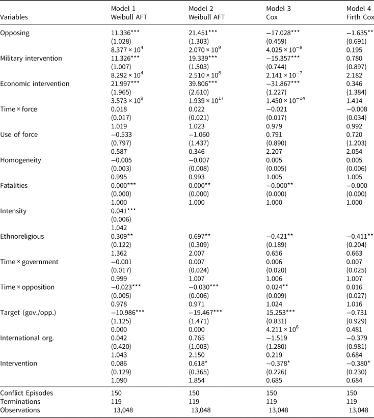
Table 2 reproduces the main findings of the article. Model 1 replicates the corresponding model from the study, which employs a Weibull duration model with an accelerated failure time (AFT) parameterization. Model 2 reports a modified version of the original specification, dropping a conflict intensity control. Model 3 employs a standard Cox model, and Model 4 adopts a Firth Cox approach.

Table 2.

Replication and extensions of Model 1, Table 1 as reported in Regan (Reference Regan2002, 69)

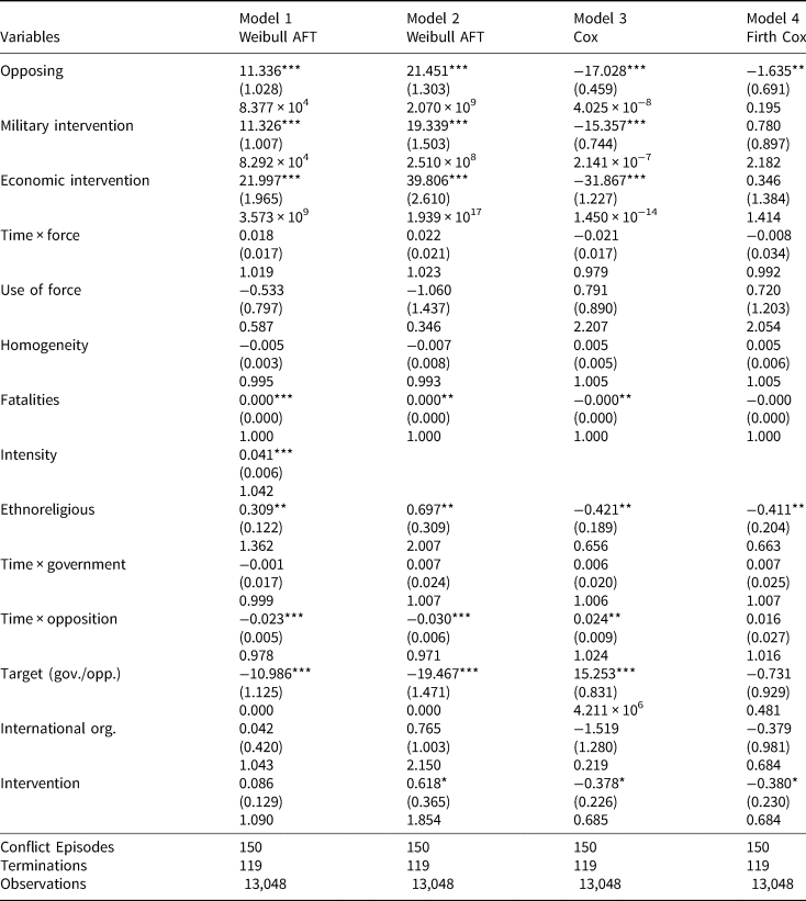
Note: Models 1–3 report variable coefficients, with robust standard errors clustered on conflict in parentheses, followed by exponentiated coefficients. Model 4 reports Firth Cox penalized maximum-likelihood estimates, with bootstrapped standard errors in parentheses, followed by exponentiated coefficients. *p ≤ 0.10; **p ≤ 0.05; ***p ≤ 0.01. All significance tests are two-tailed.

We successfully replicate the original study.Footnote ¹⁹ However, our results suggest that substantial nonconvergence issues afflict the estimated parameter values under both the Weibull AFT and standard Cox specifications. Indeed, Models 1–3 estimate extreme coefficient values for the variables recording opposing interventions, military interventions, economic interventions and biased interventions on the side of rebel forces (represented in the original study as the ‘target’ variable). The magnitude of the substantive effect of each of these variables is untenably large.

Consider first the Weibull AFT model estimates. Given the model's accelerated failure time parameterization, a positively signed coefficient implies longer expected durations. Substantive interpretation is facilitated by exponentiating the raw coefficients, which provides relative expected durations given a one-unit increase in x _i. Thus Model 1 estimates that conflicts that experience opposing interventions are over 83,000 times longer than those that do not. Likewise, conflicts that are subject to military interventions are estimated to be over 82,000 times longer, and those that experience economic interventions are estimated to be over 3,500,000,000 times longer. However, the expected duration of conflicts that receive biased interventions on the side of rebel forces is less than 0.0001 per cent that of conflicts that do not (that is, e ^−10.986). All four variables are statistically significant at conventional levels (p ≤ 0.01), but the magnitude of the substantive effects estimated by the Weibull AFT model strain credulity.

Similar results are identified in Model 2, which drops a conflict intensity control.Footnote ²⁰ The magnitude of the substantive effects for opposing interventions, military interventions, economic interventions and biased interventions on the side of rebel forces are estimated to grow even larger in this model, with time ratios converging towards infinite values. These estimates suggest considerable bias owing to monotone-likelihood conditions, with parameter values that are more a function of mathematical complications than empirical evidence.

Model 3 demonstrates that the extreme estimates we identify are not unique to duration models that adopt a Weibull AFT specification. This model re-runs the previous analysis, employing a standard Cox model. Note that because Cox models are expressed in terms of a hazard rate, interpretation of estimated coefficients is opposite that of Weibull AFT models (that is, a positively signed coefficient implies shorter expected duration). Substantive interpretation is again facilitated by exponentiating the raw coefficients, which can then be interpreted as hazard ratios. To calculate the effect of a one-unit change in x _i, one subtracts 1 from the reported hazard ratio and multiplies by 100 to recover the percent change in the hazard of conflict termination. Thus, Model 3 estimates that opposing interventions, military interventions and economic interventions all decrease the hazard of conflict termination by over 99.999 per cent. That is, these variables are estimated to virtually eliminate the likelihood of conflict termination. Biased interventions on the side of rebel forces, however, are estimated to increase the hazard of conflict termination by over 4,000,000 per cent – that is, they are estimated to virtually guarantee the end of fighting. All four variables are again statistically significant at conventional levels (p ≤ 0.01), but the size of the estimated substantive effects is impossibly large.

To explore the extent to which monotone likelihood is responsible for these extreme results, Table 3 provides an overview of imbalance on the problematic variables discussed above. We find that while 297 observations record the occurrence of opposing interventions, no observations record a conflict termination during a month when one of these opposing interventions took place. Notably, this is powerful evidence in support of Regan's hypothesis that opposing interventions prolong a conflict's expected duration. But from a methodological perspective, this means there is no overlap of failure times between conflicts that experience an opposing intervention and those that do not. Indeed, the variable is quasi-completely separating: all values opposing = 0 correspond to all termination events. Consequently, it is monotonic when ordered according to failure time, resulting in the inflated coefficient estimates reported in Table 2. This not only impedes meaningful interpretation of the effect of opposing interventions; it also induces considerable instability in parameter estimates of the model's other covariates.

Table 3.

Imbalance of problematic variables of interest

The same problem that afflicts the opposing interventions indicator can be identified for the other variables with extreme coefficient estimates. For example, while 132 observations record economic interventions, no observations record an economic intervention in the final month of a war. Here again, there is no overlap of failure times between conflicts that experience an economic intervention and those that do not;Footnote ²¹ inflated parameter values are the inevitable result. The values of the variables recording military interventions and biased interventions do not uniquely correspond to all termination events, but here too significant imbalance introduces convergence issues. Thus, while a total of 906 observations record military interventions, only nine observations saw a conflict end during one of the conflict-months experiencing these military interventions. Similarly, while a total of 986 observations record biased interventions on the side of rebel forces taking place during ongoing fighting, only nine observations record biased interventions on the side of rebel forces during the final month of a war. Given the degree of imbalance on both predictor variables, their linear combination with other covariates in the model induces monotone likelihood. The net result is extreme parameter values in the Weibull AFT and standard Cox models.

More generally, while the dataset contains a large number of observations (n = 13,048), it is also characterized by a high level of censoring. Both conditions are a function of its conflict-month data structure, which records covariate values for individual conflicts for every 1-month period.Footnote ²² This high-resolution data structure has some important strengths; for example, it enables fine-grained measurement of relevant variables over time and provides increased statistical power by increasing the number of observations included in the dataset. Yet this data structure risks introducing covariate imbalance, especially for dichotomous variables, by increasing the number of censored observations recorded on the conflict termination indicator variable. To see this, consider that of the 150 conflicts recorded in the dataset, only 119 terminated during the period of observation. In practice, this means that of the 13,048 total observations in the dataset, only 119 are coded as a conflict termination event (that is, where 0 = censored and 1 = terminated). The net result is a censoring level in excess of 99 per cent. Notably, such a high level of censoring is not uncommon: especially in duration models with time-varying covariates, higher-resolution coding procedures and data structures go hand in hand with higher levels of censoring.

To ameliorate the problem of monotone likelihood, Model 4 re-runs the analysis using a Firth Cox model, which implements penalized maximum likelihood. With this correction, the model's estimated coefficients for the imbalanced predictors are both plausible and in line with other studies. Consider the results identified for opposing interventions – the variable of interest that serves to test Regan's hypothesis that countervailing interventions are associated with longer conflict durations. The model estimates these interventions to be associated with an 80.5 per cent decrease in the hazard of conflict termination relative to conflicts that did not experience opposing interventions – a statistically significant result (p ≤ 0.01). While this estimate remains substantively large, it is in line with studies that report similar effect sizes when troops are simultaneously provided to both government and rebel forces in a conflict (Balch-Lindsay and Enterline Reference Balch-Lindsay and Enterline2000), or when civil wars become afflicted by competitive intervention (Anderson Reference Anderson2019).

The indicator variables recording military interventions, economic interventions and biased interventions on the side of rebels flip signs and are no longer statistically significant, but the estimated coefficients for all three measures no longer take on extreme values. The application of penalized maximum-likelihood estimation eliminates the convergence issues associated with these variables, providing finite parameter estimates even when confronted by the problems of monotone likelihood identified above.

In sum, we find support for Regan's hypothesis that opposing interventions generate longer civil wars. While Weibull AFT and standard Cox models estimate unrealistically large effect sizes, we correct for the problem of monotone likelihood and identify estimates that are both plausible and in line with other studies. Our application of the Firth Cox approach highlights the value of penalized maximum-likelihood estimation, which we find offers significant advantages for scholars encountering nonconvergence issues and inaccurate parameter estimates when employing duration models with imbalanced predictors.

Application 2: Partition and Peace Duration

In an important article on the prospects for peace following state partition, Tir (Reference Tir2005) examines the conditions under which countries avoid domestic conflict following their division into rump and secessionist states. Developing an argument that links partition-related factors to post-partition outcomes, he hypotheses that conflict is more likely in partitioned countries that emerge from a violent partition process (for example, Bosnia/Serbia), whereas peace is more likely in partitioned countries that emerge from a peaceful partition process (for example, Czech Republic/Slovakia). To test this proposition, he compiles a dataset of all cases of state partition that occurred during the twentieth century. Adopting a country-year format, the dataset records observations for both rump and secessionist states for each year following their partition through to 1996. A binary variable records whether the partition process was peaceful or violent; additional variables record whether the partition was ethnically based and whether the post-partition state was the secessionist (as opposed to the rump) country. Finally, a battery of controls captures the state's level of ethnic heterogeneity, its level of economic development, the coherence of its political regime and its population size.Footnote ²³

As Tir's research question seeks to identify the determinants of post-partition peace duration, the dataset records as a case of ‘failure’ those country-years that experience the termination of a peace episode (that is, the onset of domestic conflict). While the original study employs two measures of domestic conflict – the occurrence of armed conflict and the onset of civil war – we focus on the latter dependent variable, which draws on data compiled by the Correlates of War project (Sarkees Reference Sarkees2000; Small and Singer Reference Small and Singer1982).Footnote ²⁴ In total, there are 1,532 years of observation that capture forty-nine peace episodes, of which eighteen experienced peace terminations during the period of observation.

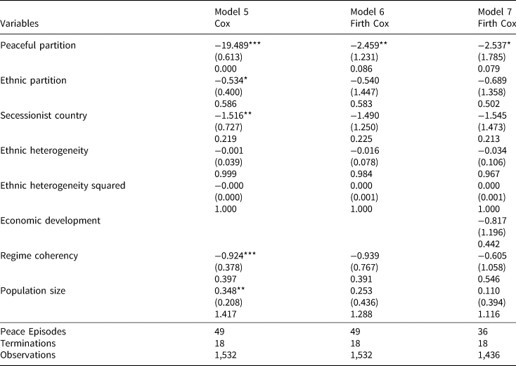
Table 4 reproduces and extends the findings of the article. Model 5 reports the original specification, which employs a standard Cox model. The results suggest that considerable nonconvergence issues afflict the parameter estimates of the independent variable of interest – the indicator for a peaceful partition process. In particular, the model estimates that peaceful partitions decrease the hazard of peace termination by over 99.999 per cent; that is, peaceful partition processes are found to virtually guarantee the continuation of peace in rump and secessionist states. These results are strongly statistically significant (p ≤ 0.01) and represent powerful evidence in support of Tir's hypothesis. However, the estimated effect sizes, which converge toward negative infinity, undermine substantive interpretation of the results.

Table 4.

Replication and extensions of Model 4, Table 1 as reported in Tir (Reference Tir2005, 556)

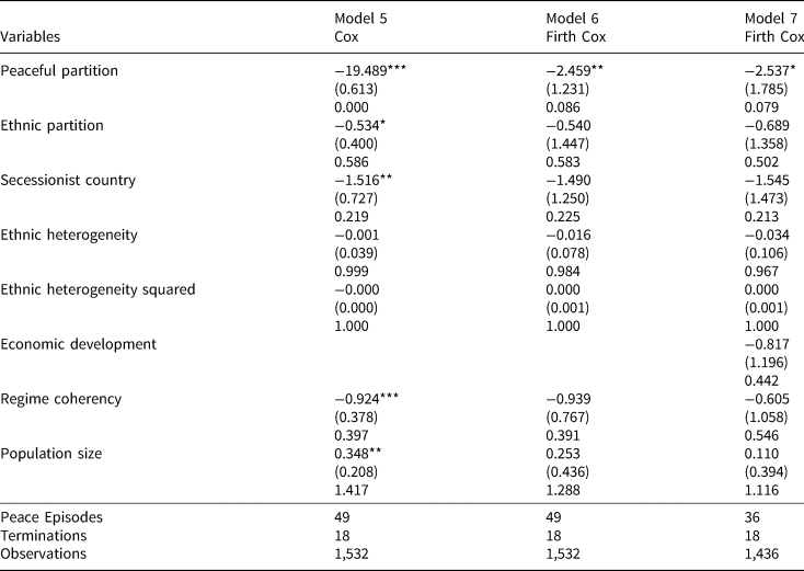
Note: Model 5 reports variable coefficients, with robust standard errors clustered on conflict in parentheses, followed by exponentiated coefficients. Models 6 and 7 report Firth Cox penalized maximum likelihood estimates, with bootstrapped standard errors in parentheses, followed by exponentiated coefficients. *p ≤ 0.10; **p ≤ 0.05; ***p ≤ 0.01. In keeping with the original study, all significance tests are one-tailed.

Is monotone likelihood to blame for the extreme effect sizes? Table 5 provides a descriptive overview of the peaceful partition indicator's degree of imbalance. We find that while a total of 485 observations record country-years that followed a peaceful partition, none of these observations saw the onset of a civil war.Footnote ²⁵ In other words, there is no overlap in failure times between cases that did and did not experience a peaceful partition, as there are no termination events associated with the value peaceful partition = 1. Consequently, the indicator variable is monotonic when ordered according to failure time. This accounts for the extreme parameter values estimated by the model.

Table 5.

Imbalance of problematic variable of interest

To solve the problem of monotone likelihood in this case, Model 6 re-runs the analysis employing a Firth Cox model. The penalized maximum-likelihood estimation ameliorates convergence issues. This model estimates that peaceful partitions are associated with a 91.4 per cent decrease in the hazard of peace termination (p ≤ 0.05). To be sure, this remains a large effect size. However, it is now both more reasonable and substantively meaningful. While monotone likelihood resulted in almost infinite effect size estimates when employing a standard Cox model, the use of penalized maximum likelihood corrects for this problem and enables the estimation of finite parameter values even in the face of highly imbalanced covariates.

Model 7 extends the analysis further, incorporating a measure of the partitioned state's level of economic development. This variable was excluded in the original article's estimated model owing to the rarity of peace terminations and missing data issues, which left insufficient variance for the joint estimation of the peaceful partition indicator and the economic development variable.Footnote ²⁶ As noted above, dropping problematic variables is one of a number of distasteful remedies scholars have in the past been forced to use when encountering monotone likelihood in their empirical research. We demonstrate the advantages of penalized maximum-likelihood estimation by (re)incorporating the economic development indicator into a fully specified model.

Our Model 7 results show that convergence issues need not force researchers to risk omitted variable bias when encountering monotone likelihood: Firth's corrective ensures finite parameter estimates can be obtained even when insufficient variance undermines the joint estimation of covariates under a standard maximum-likelihood approach. We find that the estimate of the peaceful partition indicator is robust to the incorporation of the economic development indicator, though there is greater uncertainty around this estimate in the fully specified model.

In sum, we find evidence in support of Tir's hypothesis that sustained peace is more likely in partitioned countries that emerge from a peaceful partition process. While standard Cox model estimates suffer from monotone-likelihood problems that complicate substantive interpretation of the results, we show that Firth Cox models can ameliorate this issue to render parameter estimates both meaningful and plausible. Further, while Cox models require that some variables be omitted owing to insufficient variance, we demonstrate that Firth Cox models enable researchers to avoid this distasteful remedy and estimate fully saturated models even under low-variance conditions. Here again, our results underscore the value of penalized maximum-likelihood estimation when encountering monotone likelihood in duration modeling of political events.