


1 INTRODUCTION
Suppose
$\mathbf {z}_1,\dots ,\mathbf {z}_n$
 is a random sample from the distribution of a random vector
$\mathbf {z}$
 . This article studies the large-sample properties of the following convex pairwise difference estimator:

where
$\Theta \subseteq \mathbb {R}^k$
 is a parameter space,
$\sum _{i<j}$
 denotes
$\sum _{j=2}^n \sum _{i=1}^{j-1}$
 ,
$(\mathbf {z},\bar {\mathbf {z}}) \mapsto m(\mathbf {z},\bar {\mathbf {z}};\boldsymbol {\theta })$
 is a permutation symmetric function, K is a symmetric, nonnegative kernel,
$h_n$
 is a positive bandwidth (or localization) parameter sequence,
$\mathbf {w}$
 is a continuously distributed d-dimensional subvector of
$\mathbf {z}$
 , and
$\boldsymbol {\theta } \mapsto m(\mathbf {z}_i, \mathbf {z}_j; \boldsymbol {\theta })$
 is a convex function. Pairwise difference estimation, which relies on local comparisons between observation pairs, has been used to address heterogeneity in nonlinear models. See Powell (Reference Powell, Engle and McFadden1994), Honoré and Powell (Reference Honoré, Powell, Andrews and Stock2005), and Aradillas-Lopez, Honoré, and Powell (Reference Aradillas-Lopez, Honoré and Powell2007) for overviews, and Section 2 for three motivating examples.
In contrast to classical extremum estimators,
$\widehat {\boldsymbol {\theta }}_n$
 is a local M-estimator that employs observation pairs
$(i, j)$
 for which
$\mathbf {w}_i$
 and
$\mathbf {w}_j$
 are similar. The bandwidth
$h_n$
 governs the degree of similarity: When
$h_n \to 0$
 (as
$n \to \infty $
 ), the estimator increasingly focuses on nearly-identical-in-
$\mathbf {w}$
 pairs. In turn, focusing on such pairs is natural in settings where identification can be based on the condition
$\mathbf {w}_i \approx \mathbf {w}_j$
 (combined with smoothness assumptions). The localization introduces a familiar trade-off for estimation and inference: A smaller
$h_n$
 reduces bias from dissimilarity between
$\mathbf {w}_i$
 and
$\mathbf {w}_j$
 , but increases variance due to fewer usable pairs. As a consequence, the large-sample behavior of
$\widehat {\boldsymbol {\theta }}_n$
 depends critically on a delicate bias–variance trade-off determined by
$h_n$
 . This article develops novel inference methods for convex pairwise difference estimators that are demonstrably more robust to bandwidth choice than existing methods.
Under regularity conditions and assuming that

the pairwise difference estimator
$\widehat {\boldsymbol {\theta }}_n$
 is known to be asymptotically linear:

where
$\boldsymbol {\theta }_0$
 is the estimand,
$\boldsymbol {\psi }_0(\cdot )$
 is an influence function (whose exact form is given below), and
$\rightsquigarrow $
 denotes weak convergence. Moreover, the nonparametric bootstrap approximation to the distribution in (1.3) is consistent in the sense that

where
$\widehat {\boldsymbol {\theta }}_n^{\hspace{0.5pt}*}$
 is the bootstrap analog of
$\widehat {\boldsymbol {\theta }}_n$
 and
$\rightsquigarrow _{\mathbb {P}}$
 denotes weak convergence in probability.
The main results of this article generalize (1.2)–(1.4) by combining three ideas:
-
1. Small-Bandwidth Asymptotics: Utilizing the framework introduced by Cattaneo, Crump, and Jansson (Reference Cattaneo, Crump and Jansson2014a), we obtain a Gaussian distributional approximation for the pairwise difference estimator without imposing the condition $nh_n^d \to \infty $
 , thereby allowing for higher levels of localization. This generalized distributional approximation shows in particular that, while the localization restriction
$nh_n^d \to \infty $
is necessary for establishing asymptotic linearity, a valid Gaussian approximation can be obtained under the substantially weaker condition
$n^2h_n^d\to \infty $
, albeit with a convergence rate (and approximate variance) that depends explicitly on the level of localization used.
-
2. Debiasing: Following Honoré and Powell (Reference Honoré, Powell, Andrews and Stock2005), we debias the pairwise difference estimator using the method of generalized jackknifing introduced by Schucany and Sommers (Reference Schucany and Sommers1977). Doing so allows for (larger) bandwidths that violate the bias condition $nh_n^4 \to 0$
. The same goal could be achieved by replacing the (second-order) kernel K with a higher-order kernel, but a higher-order kernel annihilates the convexity of the objective function because higher-order kernels take negative values. In contrast, generalized jackknifing retains the convexity of objective functions, which in turn is attractive for both theoretical (weaker regularity conditions) and practical (faster computation) reasons. -
3. Bootstrapping: Building on insights from Cattaneo, Crump, and Jansson (Reference Cattaneo, Crump and Jansson2014b), we develop a valid bootstrap-based distributional approximation for the debiased pairwise difference estimator by rescaling the localization parameter. The nonparametric bootstrap distributional approximation exhibits a mismatch in its asymptotic variance under small-bandwidth asymptotics. The mismatch is characterized by a known multiplicative factor involving the localization parameter $h_n$
. As a result, bootstrapping the (debiased) pairwise difference estimator with a different localization parameter (namely,
$3^{1/d}h_n$
rather than
$h_n$
) leads to a valid bootstrap-based inference procedure also under small-bandwidth asymptotics.


In combination, these three ideas enable us to offer a novel resampling-based inference method for (convex) pairwise difference estimators that is demonstrably more robust to the choice of the localization parameter
$h_n$
 than methods based on (1.2)–(1.4).
Our theoretical work is carefully developed to retain and leverage convexity of the objective function defining the pairwise difference estimator. This feature not only allows for fast implementation of the estimator and resampling-based methods, but also enables us to proceed under relatively weak conditions when obtaining theoretical results. When developing our theoretical results, we rely heavily on the foundational work of Hjort and Pollard (Reference Hjort and Pollard1993) and Pollard (Reference Pollard1991), which we apply to the case of U-processes.
This article is connected to several strands of the literature. Contributions to the pairwise difference estimation literature include Ahn et al. (Reference Ahn, Ichimura, Powell and Ruud2018), Ahn and Powell (Reference Ahn and Powell1993), Aradillas-Lopez (Reference Aradillas-Lopez2012), Blundell and Powell (Reference Blundell and Powell2004), Hong and Shum (Reference Hong and Shum2010), Honoré (Reference Honoré1992), Honoré, Kyriazidou, and Udry (Reference Honoré, Kyriazidou and Udry1997), Honoré and Powell (Reference Honoré and Powell1994), Jochmans (Reference Jochmans2013), Kyriazidou (Reference Kyriazidou1997), and Powell (Reference Powell, Hsiao, Morimune and Powell2001). The theoretical and practical features of small-bandwidth asymptotics, and their connection with resampling methods for inference, are discussed in Cattaneo, Crump, and Jansson (Reference Cattaneo, Crump and Jansson2010); Cattaneo et al. (Reference Cattaneo, Crump and Jansson2014a, Reference Cattaneo, Crump and Jansson2014b), Cattaneo et al. (Reference Cattaneo, Farrell, Jansson and Masini2025), Cattaneo and Jansson (Reference Cattaneo and Jansson2018, Reference Cattaneo and Jansson2022), Cattaneo, Jansson, and Newey (Reference Cattaneo, Jansson and Newey2018), Matsushita and Otsu (Reference Matsushita and Otsu2021), and references therein. The generalized jackknife has been successfully used for debiasing in density weighted average derivative estimation (Powell, Stock, and Stoker, Reference Powell, Stock and Stoker1989), asymptotically linear pairwise difference estimation (Honoré and Powell, Reference Honoré, Powell, Andrews and Stock2005), nonlinear semiparametric estimation (Cattaneo, Crump, and Jansson, Reference Cattaneo, Crump and Jansson2013), monotone estimation (Cattaneo, Jansson, and Nagasawa, Reference Cattaneo, Jansson and Nagasawa2024), and random forest estimation (Cattaneo, Klusowski, and Underwood, Reference Cattaneo, Klusowski and Underwood2026), among other settings. Shao and Tu (Reference Shao and Tu2012) give a textbook introduction to jackknifing, bootstrapping, and other resampling methods.
The rest of the article proceeds as follows. Section 2 introduces the three examples that are used throughout the article to motivate our work and to illustrate the verification of the high-level assumptions imposed. Section 3 presents our main results. The proofs of these results are given in Section 4. Section 5 revisits the three motivating examples and gives primitive conditions under which these examples are covered by our general theory. Simulation evidence is reported in Section 6. Section 7 gives final remarks.
2 MOTIVATING EXAMPLES
We use three examples to motivate and illustrate our work. The first example involves an estimator that can be written in closed form (because it has a quadratic-in-
$\boldsymbol {\theta }$
 function
$m(\mathbf {z}_i, \mathbf {z}_j; \boldsymbol {\theta })$
 ), while the other two examples do not. The second example has a smooth-in-
$\boldsymbol {\theta }$
 function
$m(\mathbf {z}_i, \mathbf {z}_j; \boldsymbol {\theta })$
 , while the third example does not. All three examples have convex-in-
$\boldsymbol {\theta }$
 functions
$m(\mathbf {z}_i, \mathbf {z}_j; \boldsymbol {\theta })$
 and employ the following notation:
$\mathbf {z}_i = (y_i, \mathbf {x}_i', \mathbf {w}_i')'$
 , with
$y_i$
 a scalar outcome variable,
$\mathbf {x}_i$
 a k-dimensional covariate, and
$\mathbf {w}_i$
 a d-dimensional covariate. For more details on the examples, see Powell (Reference Powell, Engle and McFadden1994), Honoré and Powell (Reference Honoré, Powell, Andrews and Stock2005), and Aradillas-Lopez et al. (Reference Aradillas-Lopez, Honoré and Powell2007).
2.1 Partially Linear Regression Model
The partially linear regression model is of the form

where
$\boldsymbol {\theta }_0$
 is the parameter of interest,
$\gamma _0(\cdot )$
 is an unknown function, and where
$\mathbb {E}[\varepsilon _i|\mathbf {x}_i,\mathbf {w}_i]=0$
 . Defining
$\dot {y}_{i,j}=y_i-y_j$
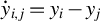 and
$\dot {\mathbf {x}}_{i,j}=\mathbf {x}_i-\mathbf {x}_j$
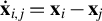 , a pairwise difference estimator of
$\boldsymbol {\theta }_0$
 can be based on

Setting
$\Theta =\mathbb {R}^k$
 , the minimization problem in (1.1) admits a closed-form solution (provided that a nonnegative kernel function is used), namely,

2.2 Partially Linear Logit Model
The partially linear logit model studied here is of the form

where
$\boldsymbol {\theta }_0$
 is the parameter of interest,
$\gamma _0(\cdot )$
 is an unknown function, and

The parameter
$\boldsymbol {\theta }_0$
 can be estimated using a pairwise difference estimator with
$\Theta =\mathbb {R}^k$
 and

The minimization problem in (1.1) does not admit a closed-form solution, but it is convex (provided that a nonnegative kernel function is used) because
$u\mapsto -\ln \Lambda (u)$
 is.
2.3 Partially Linear Tobit Model
The partially linear censored regression model studied here is of the form

where
$\boldsymbol {\theta }_0$
 is the parameter of interest,
$\gamma _0(\cdot )$
 is an unknown function,
$x_i \perp\!\!\perp \varepsilon_i \mid w_i$
 , and the conditional distribution of
$\varepsilon _i$
 given
$\mathbf {w}_i$
 admits a Lebesgue density. A pairwise difference estimator of
$\boldsymbol {\theta }_0$
 can be obtained by setting
$\Theta =\mathbb {R}^k$
 and employing

where

Because
$\tilde {m}_{\mathtt {PLT}}(\mathbf {z}_i,\mathbf {z}_j;\boldsymbol 0)$
 does not depend on
$\boldsymbol {\theta }$
 , its presence in
$m_{\mathtt {PLT}}(\mathbf {z}_i,\mathbf {z}_j;\boldsymbol {\theta })$
 does not affect the minimization problem defining the estimator. Nevertheless, it is theoretically attractive to work with
$m_{\mathtt {PLT}}$
 rather than
$\tilde {m}_{\mathtt {PLT}}$
 , as doing so allows for weaker regularity conditions for the existence of the expectation of the objective function.
For future reference, we note that
$m_{\mathtt {PLT}}$
 admits the alternative representation

The function
$\boldsymbol {\theta }\mapsto m_{\mathtt {PLT}}(\mathbf {z}_1,\mathbf {z}_2;\boldsymbol {\theta })$
 is convex and therefore so is the minimization problem in (1.1) (provided that a nonnegative kernel function is used).
3 DISTRIBUTIONAL APPROXIMATION AND BOOTSTRAP INFERENCE
As is standard in the literature, we generalize (1.1) slightly and define our estimator
$\widehat {\boldsymbol {\theta }}_n=\widehat {\boldsymbol {\theta }}_n(h_n)$
 to be any approximate minimizer of
$\widehat {M}_n(\boldsymbol {\theta };h_n)$
 , where

To be specific, we require

The objective function
$\widehat {M}_n$
 is a sample counterpart of the function M given by

Under regularity conditions, this function approximates, as
$h\downarrow 0$
 , a function
$M_0$
 , which (does not depend on K and) admits a unique minimizer, namely, the parameter of interest
$\boldsymbol {\theta }_0$
 .
For the purposes of analyzing
$\widehat {\boldsymbol {\theta }}_n$
 , it is convenient to define
$\boldsymbol {\theta }_n = \boldsymbol {\theta }(h_n)$
 , where

is interpretable as a (fixed-h) “pseudo” parameter. With the help of
$\boldsymbol {\theta }_n$
 , we can decompose the estimation error
$\widehat {\boldsymbol {\theta }}_n-\boldsymbol {\theta }_0$
 into a (non-stochastic) “bias” component
$\boldsymbol {\theta }_n-\boldsymbol {\theta }_0$
 and a “noise” component
$\widehat {\boldsymbol {\theta }}_n-\boldsymbol {\theta }_n$
 . Each component can be analyzed separately, and in both cases, the analysis will leverage convexity.
3.1 Regularity Conditions
The following assumption guarantees, among other things, that
$\boldsymbol {\theta }_n$
 is well defined for large n and that the bias component
$\boldsymbol {\theta }_n-\boldsymbol {\theta }_0$
 vanishes asymptotically; for details, see Lemma 1 of Section 4.1.
Assumption 1.
-
(i) The kernel function K is a symmetric, bounded probability density.
-
(ii) $\Theta \subseteq \mathbb {R}^k$
is convex,
$(\mathbf {z},\bar {\mathbf {z}}) \mapsto m(\mathbf {z},\bar {\mathbf {z}};\boldsymbol {\theta })$
is permutation symmetric, and
$\boldsymbol {\theta } \mapsto m(\mathbf {z}_1,\mathbf {z}_2;\boldsymbol {\theta })$
is convex with probability one. -
(iii) The distribution of $\mathbf {w}$
admits a Lebesgue density
$f_{\mathbf {w}}$
, which is bounded and continuous on its support
$\mathcal {W}$
. -
(iv) For each $\boldsymbol {\theta }\in \Theta $
, $$ \begin{align*} \mathbb{E}\left[\sup_{\mathbf{w}_2\in\mathcal{W}}|\mathbb{E}[m(\mathbf{z}_1,\mathbf{z}_2;\boldsymbol{\theta})|\mathbf{w}_1,\mathbf{w}_2]|f_{\mathbf{w}}(\mathbf{w}_2)\right]<\infty \end{align*} $$and (with probability one)
$$ \begin{align*} \lim_{\mathbf{u}\to \mathbf{0}} \mathbb{E}[m(\mathbf{z}_1,\mathbf{z}_2;\boldsymbol{\theta})|\mathbf{w}_1=\mathbf{w},\mathbf{w}_2=\mathbf{w}+\mathbf{u}] = \mathbb{E}[m(\mathbf{z}_1,\mathbf{z}_2;\boldsymbol{\theta})|\mathbf{w}_1=\mathbf{w},\mathbf{w}_2=\mathbf{w}]. \end{align*} $$
-
(v) On $\Theta $
, the function
$M_0$
given by $$ \begin{align*} M_0(\boldsymbol{\theta}) = \int_{\mathcal{W}} \mathbb{E}[m(\mathbf{z}_1,\mathbf{z}_2;\boldsymbol{\theta})|\mathbf{w}_1=\mathbf{w},\mathbf{w}_2=\mathbf{w}]f_{\mathbf{w}}(\mathbf{w})^2d\mathbf{w} \end{align*} $$is uniquely minimized at an interior point $\boldsymbol {\theta }_0$
.





The next assumption enables us to analyze the asymptotic properties of the noise component
$\widehat {\boldsymbol {\theta }}_n-\boldsymbol {\theta }_n$
 . To accommodate examples (such as the partially linear Tobit model) where
$\boldsymbol {\theta } \mapsto m(\mathbf {z}_i,\mathbf {z}_j;\boldsymbol {\theta })$
 is not fully differentiable, we assume the existence of derivative-like functions
$\mathbf {s}(\mathbf {z}_i,\mathbf {z}_j;\boldsymbol {\theta })\in \mathbb {R}^k$
 and
$\mathbf {H}(\mathbf {w}_i,\mathbf {w}_j;\boldsymbol {\theta },\mathbf {t})\in \mathbb {R}^{k\times k}$
 such that, for any direction
$\mathbf {t} \in \mathbb {R}^k$
 , the (remainder) terms

and

are suitably small for
$\boldsymbol {\theta }$
 near
$\boldsymbol {\theta }_0$
 ,
$\tau>0$
 near zero, and
$\mathbf {w}_1 \approx \mathbf {w}_2$
 . As further discussed below, functions
$\mathbf {s}$
 and
$\mathbf {H}$
 satisfying the following assumption exist (and are relatively easy to find) in each of our motivating examples.
Assumption 2.
-
(i) For each $\mathbf {t} \in \mathbb {R}^k$
, there is some
$\delta>0$
such that $$ \begin{align*} & \mathbb{E}\left[\sup_{ \tau\in (0,\delta),\|\boldsymbol{\theta}-\boldsymbol{\theta}_0\|<\delta, \mathbf{w}_2 \in\mathcal{W}} \left|\mathbb{E}[ r_{\mathbf{t}}(\boldsymbol{\theta},\tau) | \mathbf{z}_1,\mathbf{w}_2 ] \right|f_{\mathbf{w}}(\mathbf{w}_2)^2 \right]< \infty,\\ & \mathbb{E}\left[\sup_{ \tau\in (0,\delta),\|\boldsymbol{\theta}-\boldsymbol{\theta}_0\|<\delta, \mathbf{w}_2 \in\mathcal{W}} \mathbb{E}[r_{\mathbf{t}}(\boldsymbol{\theta},\tau)^2 | \mathbf{w}_1,\mathbf{w}_2 ] f_{\mathbf{w}}(\mathbf{w}_2) \right] < \infty,\\ &\mathbb{E}\left[\sup_{\tau\in (0,\delta),\|\boldsymbol{\theta}-\boldsymbol{\theta}_0\|<\delta, \mathbf{w}_2 \in\mathcal{W}} \left|R_{\mathbf{t}}(\boldsymbol{\theta},\tau)\right| f_{\mathbf{w}}(\mathbf{w}_2) \right]<\infty, \end{align*} $$and (with probability one)
$$ \begin{align*} & \lim_{\tau\downarrow0,(\boldsymbol{\theta},\mathbf{u})\to(\boldsymbol{\theta}_0,\mathbf{0})} \mathbb{E}[ r_{\mathbf{t}}(\boldsymbol{\theta},\tau) | \mathbf{z}_1=\mathbf{z},\mathbf{w}_2 =\mathbf{w}+\mathbf{u} ] = 0, \\ & \lim_{\tau\downarrow0,(\boldsymbol{\theta},\mathbf{u})\to(\boldsymbol{\theta}_0,\mathbf{0})} \mathbb{E}[ r_{\mathbf{t}}(\boldsymbol{\theta},\tau)^2 | \mathbf{w}_1=\mathbf{w},\mathbf{w}_2=\mathbf{w}+\mathbf{u} ] = 0, \\ & \lim_{\tau\downarrow0,(\boldsymbol{\theta},\mathbf{u})\to(\boldsymbol{\theta}_0,\mathbf{0})} \mathbb{E}[ R_{\mathbf{t}}(\boldsymbol{\theta},\tau) | \mathbf{w}_1=\mathbf{w},\mathbf{w}_2 =\mathbf{w}+\mathbf{u} ] = 0. \end{align*} $$
-
(ii) There is some $\delta>0$
and some function b with $$ \begin{align*} \sup_{\|\boldsymbol{\theta}-\boldsymbol{\theta}_0\|<\delta} \|\mathbf{s}(\mathbf{z}_1,\mathbf{z}_2;\boldsymbol{\theta})\|\leq b(\mathbf{z}_1)b(\mathbf{z}_2), \end{align*} $$such that
$$ \begin{align*} \mathbb{E}[b(\mathbf{z})^4] + \sup_{\mathbf{w}\in\mathcal{W}}\mathbb{E}[b(\mathbf{z})^4|\mathbf{w}]f_{\mathbf{w}}(\mathbf{w})<\infty \end{align*} $$and
$$ \begin{align*} \mathbb{E}\left[\sup_{\|\boldsymbol{\theta}-\boldsymbol{\theta}_0\|<\delta, \mathbf{w}_2\in\mathcal{W}} \|\mathbf{H}(\mathbf{w}_1,\mathbf{w}_2;\boldsymbol{\theta},\mathbf{t})\| f_{\mathbf{w}}(\mathbf{w}_2) \right] < \infty \qquad \text{for each } \mathbf{t} \in \mathbb{R}^k. \end{align*} $$
-
(iii) There exist functions $\mathbf {G}_0,\boldsymbol {\xi }_0$
, and
$\boldsymbol {\Xi }_0$
such that, for each
$\mathbf {t}\in \mathbb {R}^k$
(and with probability one), $$ \begin{align*} \lim_{(\boldsymbol{\theta},\mathbf{u})\to(\boldsymbol{\theta}_0,\mathbf{0})} \mathbf{H}(\mathbf{w},\mathbf{w}+\mathbf{u};\boldsymbol{\theta},\mathbf{t}) f_{\mathbf{w}}(\mathbf{w}) = \mathbf{G}_0(\mathbf{w}), \end{align*} $$
$$ \begin{align*} \lim_{(\boldsymbol{\theta},\mathbf{u})\to(\boldsymbol{\theta}_0,\mathbf{0})} -2\mathbb{E}[\mathbf{s}(\mathbf{z}_1,\mathbf{z}_2;\boldsymbol{\theta})|\mathbf{z}_1=\mathbf{z},\mathbf{w}_2=\mathbf{w}+\mathbf{u} ] f_{\mathbf{w}}(\mathbf{w}) = \boldsymbol{\xi}_0(\mathbf{z}), \end{align*} $$and
$$ \begin{align*} \lim_{(\boldsymbol{\theta},\bar{\boldsymbol{\theta}},\mathbf{u})\to (\boldsymbol{\theta}_0,\boldsymbol{\theta}_0,\mathbf{0}) } \mathbb{E}[\mathbf{s}(\mathbf{z}_1,\mathbf{z}_2;\boldsymbol{\theta})\mathbf{s}(\mathbf{z}_1,\mathbf{z}_2;\bar{\boldsymbol{\theta}})'|\mathbf{w}_1=\mathbf{w},\mathbf{w}_2=\mathbf{w}+\mathbf{u} ] f_{\mathbf{w}}(\mathbf{w})= \boldsymbol{\Xi}_0(\mathbf{w}). \end{align*} $$
-
(iv) $\boldsymbol {\Gamma }_0 = \mathbb {E}[\mathbf {G}_0(\mathbf {w})], \boldsymbol {\Sigma }_0 = \mathbb {E}[\boldsymbol {\xi }_0(\mathbf {z})\boldsymbol {\xi }_0(\mathbf {z})']$
, and
$\mathbb {E}[\boldsymbol {\Xi }_0(\mathbf {w})]$
are positive definite.




3.2 Small-Bandwidth Asymptotics
Defining

and letting
$\Phi _k$
 denote the distribution function of a k-dimensional standard Gaussian random vector, we have the following result.
Theorem 1. Suppose Assumptions 1 and 2 hold. If
$n^2h_n^d\to \infty $
 and if
$h_n\to 0$
 , then

Under the assumptions of Theorem 1, the convergence rate of
$\widehat {\boldsymbol {\theta }}_n-\boldsymbol {\theta }_n$
 is given by the magnitude of
$\mathbf {V}_n^{-1/2}$
 , namely,

Provided that the bias is “small” in the sense that
$\rho _n\|\boldsymbol {\theta }_n-\boldsymbol {\theta }_0\|\to 0$
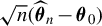
 , Theorem 1 therefore encompasses the following three distinct large-sample regimes:
-
• Asymptotic Linearity: If $nh_n^d\to \infty $
, then
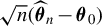
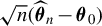
$\sqrt {n}(\widehat {\boldsymbol {\theta }}_n-\boldsymbol {\theta }_0)$
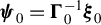
satisfies (1.3) with
$\boldsymbol {\psi }_0 = \boldsymbol {\Gamma }_0^{-1}\boldsymbol {\xi }_0$
. In particular,
$\sqrt {n}(\widehat {\boldsymbol {\theta }}_n-\boldsymbol {\theta }_0)$
converges in law to a centered Gaussian distribution with variance $$ \begin{align*} \lim_{n\to\infty} n \mathbf{V}_n(h_n) = \boldsymbol{\Gamma}_0^{-1} \boldsymbol{\Sigma}_0 \boldsymbol{\Gamma}_0^{-1}. \end{align*} $$
-
• Root-n Consistency without Asymptotic Linearity: If $nh_n^d\to 2c \in (0,\infty )$
, then
$\widehat {\boldsymbol {\theta }}_n$
is not asymptotically linear, but it is
$\sqrt {n}$
-consistent,
$\sqrt {n}(\widehat {\boldsymbol {\theta }}_n-\boldsymbol {\theta }_0)$
converging in law to a centered Gaussian distribution with variance $$ \begin{align*} \lim_{n\to\infty} n \mathbf{V}_n(h_n) = \boldsymbol{\Gamma}_0^{-1}\left[ \boldsymbol{\Sigma}_0 + \frac{1}{c} \boldsymbol{\Delta}_0(K)\right]\boldsymbol{\Gamma}_0^{-1}. \end{align*} $$
-
• Slower than Root-n Consistency: If $nh_n^d\to 0$
(but
$n^2h_n^d\to \infty $
), then
$\widehat {\boldsymbol {\theta }}_n$
is neither asymptotically linear nor
$\sqrt {n}$
-consistent, but
$\sqrt {n^2h_n^d/2}(\widehat {\boldsymbol {\theta }}_n-\boldsymbol {\theta }_0)$
converges in law to a centered Gaussian distribution with variance $$ \begin{align*} \lim_{n\to\infty} \binom{n}{2}h_n^d \mathbf{V}_n(h_n) = \boldsymbol{\Gamma}_0^{-1}\boldsymbol{\Delta}_0(K)\boldsymbol{\Gamma}_0^{-1}. \end{align*} $$









The small-bandwidth component (i.e., the term involving
$\boldsymbol {\Delta }_0(K)$
 ) in
$\mathbf {V}_n$
 captures the additional estimation uncertainty generated from increasing the localization of the observation pairs. Incorporating this component in the approximate variance is key to enabling us to replace the condition
$nh_n^d\to \infty $
 by the weaker condition
$n^2h_n^d\to \infty $
 when obtaining a Gaussian approximation. As demonstrated by Cattaneo et al. (Reference Cattaneo, Farrell, Jansson and Masini2025) in a related context, incorporating the small-bandwidth component can furthermore lead to a more accurate distributional approximation (in a higher-order asymptotic sense) even under asymptotic linearity.
3.3 Debiasing
In Theorem 1, we centered the estimator
$\widehat {\boldsymbol {\theta }}_n=\widehat {\boldsymbol {\theta }}_n(h_n)$
 at
$\boldsymbol {\theta }_n=\boldsymbol {\theta }(h_n)$
 to circumvent bias issues. This section focuses on the bias term
$\boldsymbol {\theta }_n-\boldsymbol {\theta }_0$
 and introduces an automatic debiasing approach under the assumption that
$\boldsymbol {\theta }_n-\boldsymbol {\theta }_0$
 can be expanded in even powers of
$h_n$
 . To be specific, we follow Honoré and Powell (Reference Honoré, Powell, Andrews and Stock2005, Section 3.3) and discuss debiasing under the following high-level condition.
Assumption 3. For some even
$\mathtt {S} \geq 0$
 ,
$\boldsymbol {\theta }(\cdot )$
 admits
$\mathbf {b}_{2l}\in \mathbb {R}^k$
 (for
$l=1,\dots , \mathtt {S}/2$
 ) such that

The ease with which Assumption 3 can be verified depends on the magnitude of
$\mathtt {S}$
 . For instance, Assumption 1 implies that Assumption 3 holds with
$\mathtt {S}=0$
 . Under additional smoothness conditions and using symmetry of K, the following result gives conditions under which Assumption 3 holds with
$\mathtt {S}=2$
 . When stating the result, we employ the following standard multi-index notation: for
$\boldsymbol {\nu } = (\nu _1,\ldots ,\nu _d)'\in \mathbb {Z}_+^d$
 ,
$\bar {\mathbf {w}} = (\bar {w}_1,\ldots ,\bar {w}_d)'\in \mathbb {R}^d$
 , and a sufficiently smooth-in-
$\bar {\mathbf {w}}$
 function
$f(\mathbf {w},\bar {\mathbf {w}}),$


Proposition 1. Suppose Assumptions 1 and 2 hold and that
-
(i) $\int _{\mathbb {R}^d} \|\mathbf {u}\|^2 K(\mathbf {u})d\mathbf {u}<\infty $
, and -
(ii) with probability one, $\bar {\mathbf {w}} \mapsto \boldsymbol {\varphi }(\mathbf {w},\bar {\mathbf {w}}) = \mathbb {E}[\mathbf {s}(\mathbf {z}_1,\mathbf {z}_2;\boldsymbol {\theta }_0)|\mathbf {w}_1=\mathbf {w},\mathbf {w}_2=\bar {\mathbf {w}}]f_{\mathbf {w}}(\bar {\mathbf {w}})$
is twice continuously differentiable with
$\mathbb {E}[\sup _{\bar {\mathbf {w}}\in \mathcal {W}}\|\partial _{\bar {\mathbf {w}}}^{\boldsymbol {\nu }} \boldsymbol {\varphi }(\mathbf {w},\bar {\mathbf {w}})\|]<\infty $
for all
$\boldsymbol {\nu }\in \mathbb {Z}_+^d$
with
$|\boldsymbol {\nu }|\leq 2$
.





Then
$\boldsymbol {\theta }(\cdot )$
 admits a
$\mathbf {b}_2\in \mathbb {R}^k$
 such that

The proof of Proposition 1 leverages convexity and may therefore be of independent interest. The convexity argument in question can furthermore be adapted to form the basis of a verification by induction of Assumption 3 with
$\mathtt {S}>2$
 . Details are provided in Section 4.4, which describes the induction step for general
$\mathtt {S}$
 and states explicit (smoothness) conditions under which Assumption 3 holds with
$\mathtt {S} =4$
 .
To describe the debiasing procedure based on generalized jackknifing, we maintain Assumption 3, define
$c_0=1$
 , choose a nonnegative integer L, and let
$\mathbf {c}=(c_0,\dots , c_{L})'$
 be a vector of (distinct) positive constants such that the following vector is well defined:

The debiased estimator is

the construction of which involves solving
$L+1$
 convex optimization problems. As defined, the debiased estimator is a generalization of the original pairwise difference estimator because if
$L=0$
 , then
$\mathbf {c}=1=\lambda _0$
 and therefore
$\widetilde {\boldsymbol {\theta }}_n = \widehat {\boldsymbol {\theta }}_n$
 .
The next theorem generalizes Theorem 1 by establishing the small-bandwidth Gaussian approximation for
$\widetilde {\boldsymbol {\theta }}_n$
 . To state the theorem, let

and

As they should, the expressions have the feature that if
$L=0$
 , then
$\bar {\boldsymbol {\theta }}_n = \boldsymbol {\theta }_n$
 and
$\bar {\mathbf {V}}_n=\mathbf {V}_n$
 . Another noteworthy feature of the expressions is that debiasing via generalized jackknifing affects the variance
$\bar {\mathbf {V}}_n$
 only through the kernel shape entering its small-bandwidth component.
Theorem 2. Suppose Assumptions 1 and 2 hold. If
$n^2h_n^d\to \infty $
 and if
$h_n\to 0$
 , then

As a consequence, if Assumption 3 also holds with
$\mathtt {S} \geq 2L+2$
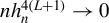
 , and if
$nh_n^{4(L+1)}\to 0$
 , then

The magnitude of
$\bar {\mathbf {V}}_n^{-1/2}$
 is the same as that of
$\mathbf {V}_n^{-1/2}$
 . With obvious modifications, the discussion of
$\widehat {\boldsymbol {\theta }}_n$
 following Theorem 1 therefore applies to
$\widetilde {\boldsymbol {\theta }}_n$
 , the only noteworthy difference being that (by design) the relevant “small bias” condition is different (and typically milder) in the case of
$\widetilde {\boldsymbol {\theta }}_n$
 .
When
$L=0$
 (i.e., one uses the original pairwise difference estimator), the second part of Theorem 2 imposes
$nh_n^4\to 0$
 , which coincides with the standard small bias condition in (1.2), while the first part of the theorem still accommodates the small-bandwidth distributional approximation.
It is worth noting that for
$L\geq 1$
 , the equivalent kernel
$\bar {K}$
 is of higher order, even though the debiased estimator
$\widetilde {\boldsymbol {\theta }}_n$
 only employs estimators constructed using second-order kernels, thereby retaining the desired convexity for implementation. To be specific, if
$\int _{\mathbb {R}^d} \|\mathbf {u}\|^{2L+2} K(\mathbf {u})d\mathbf {u} < \infty $
 , then
$\bar {K}$
 is of order
$2L+2$
 because

and, for
$\boldsymbol {\nu }=(\nu _1,\dots ,\nu _d)'\in \mathbb {Z}^d_+$
 with
$0<|\boldsymbol {\nu }|\leq 2L+1$
 ,

where the last equality uses the defining property of
$\{\lambda _l(\mathbf {c})\}$
 and symmetry of K, and
$\mathbf {u}^{\boldsymbol {\nu }}$
 denotes
$\prod _{j=1}^d u_j^{\nu _j}$
 for
$\mathbf {u}=(u_1,\dots ,u_d)'\in \mathbb {R}^d$
 .
3.4 Bootstrapping
To develop feasible inference procedures that do not require (explicit) estimation of
$\bar {\mathbf {V}}_n$
 , we consider nonparametric bootstrap-based approximations to the distribution of
$\widetilde {\boldsymbol {\theta }}_n$
 . (Since
$\widetilde {\boldsymbol {\theta }}_n=\widehat {\boldsymbol {\theta }}_n$
 when
$L=0$
 , results for
$\widehat {\boldsymbol {\theta }}_n$
 can be extracted by setting
$L=0$
 in what follows.)
Letting
$\mathbf {z}^{\hspace{0.5pt}*}_{1,n},\dots ,\mathbf {z}^{\hspace{0.5pt}*}_{n,n}$
 denote a random sample from the empirical distribution of
$\mathbf {z}_1,\dots ,\mathbf {z}_n$
 , the defining property of
$\widehat {\boldsymbol {\theta }}_n^{\hspace{0.5pt}*}(h)$
 , the nonparametric bootstrap analog of
$\widehat {\boldsymbol {\theta }}_n(h)$
 , is the following:

where

Similarly, the nonparametric bootstrap analog of
$\widetilde {\boldsymbol {\theta }}_n$
 is

The following theorem characterizes the large sample properties of
$\widetilde {\boldsymbol {\theta }}_n^{\hspace{0.5pt}*}-\widetilde {\boldsymbol {\theta }}_n$
 , the bootstrap counterpart of
$\widetilde {\boldsymbol {\theta }}_n-\bar {\boldsymbol {\theta }}_n$
 . In perfect analogy with the results in Cattaneo et al. (Reference Cattaneo, Crump and Jansson2014b), we find that the bootstrap distribution estimator is consistent only when
$nh_n^d\to \infty $
 , but otherwise exhibits a variance inflation making the distributional approximation inconsistent. To state the result, let
$\mathbb {P}_n^{\hspace{0.5pt}*}[\cdot ]$
 denote
$\mathbb {P}[\cdot | \mathbf {z}_1,\ldots ,\mathbf {z}_n]$
 , let
$\to _{\mathbb {P}}$
 denote convergence in probability, and define

Theorem 3. Suppose Assumptions 1 and 2 hold and that, for
$\boldsymbol {\theta }$
 near
$\boldsymbol {\theta }_0$
 (and with probability one),
$m(\mathbf {z},\mathbf {z};\boldsymbol {\theta })=0$
 and
$\mathbf {s}(\mathbf {z},\mathbf {z};\boldsymbol {\theta })=\mathbf {0}$
 . If
$n^2h_n^d\to \infty $
 and if
$h_n\to 0$
 , then

Because
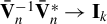
$\bar {\mathbf {V}}_n^{-1}\bar {\mathbf {V}}_n^{\hspace{0.5pt}*}\to \mathbf {I}_k$
 if and only if
$nh_n^d\to \infty $
 (where
$\mathbf {I}_k$
 denotes the k-dimensional identity matrix), under the assumptions of Theorem 3,

if and only if
$nh_n^d\to \infty $
 . In particular, if
$\liminf _{n\to \infty } nh_n^d<\infty $
 , then the nonparametric bootstrap is inconsistent, albeit conservative in the sense that the (approximate) variance under the bootstrap distribution is larger than the (approximate) variance of the asymptotic distribution:
$\bar {\mathbf {V}}_n^{\hspace{0.5pt}*}> \bar {\mathbf {V}}_n$
 in a positive-definite sense.
The variance inflation problem associated with the nonparametric bootstrap under the small-bandwidth regime can be easily fixed by appropriately rescaling the bandwidth used for the bootstrap implementation of the pairwise difference estimator. Employing

and centering its distribution at

automatically adjusts the bootstrap variance, leading to a consistent distributional approximation. Indeed, the following result is an immediate consequence of Theorems 2 and 3.
Corollary 1. If the assumptions of Theorem 3 hold, then

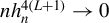
As a consequence, if Assumption 3 also holds with
$\mathtt {S} \geq 2L+2$
 , and if
$nh_n^{4(L+1)}\to 0$
 , then

The statement of Corollary 1 emphasizes the rate-adaptive nature of the consistency property enjoyed by the bootstrap distributional approximation.
3.5 Discussion
Our results provide a simple practical message: bootstrap-based inference for convex pairwise difference estimators is highly sensitive to bandwidth choice under conventional implementations, but this sensitivity can be substantially reduced by combining debiasing with a bandwidth rescaling. In particular, the classical bootstrap is valid only over a relatively narrow range of bandwidth sequences, whereas generalized jackknifing enlarges the set of admissible large bandwidths, small-bandwidth asymptotics justifies an implementation enlarging the set of admissible small bandwidths, and the combination of the two yields the broadest range of valid inference.
To summarize these conclusions, suppose
$\mathtt {S}\geq 2L+2$
 , let
$\alpha \in (0,1)$
 and
$\mathbf {a}\in \mathbb {R}^k$
 be fixed, and consider the following family of percentile bootstrap confidence intervals (in the terminology of van der Vaart, Reference van der Vaart1998) for
$\mathbf {a}'\boldsymbol {\theta }_0$
 :

where

The notation highlights the two tuning parameters that vary across the different inference procedures: given a choice of bandwidth h used in the point estimator, the scaling constant B used in the bootstrap approximation, and the debiasing order
$L=\dim (\mathbf {c})-1$
 , which together with
$\mathbf {c}$
 determines the generalized jackknife weights.
To sharpen the practical interpretation of these conclusions, it is useful to view each procedure through its coverage function

Our theory implies that the main differences across procedures can be understood in terms of how
$\mathsf {CF}_{n,1-\alpha }(B,L)$
 behaves as the bandwidth sequence moves from the small-bandwidth region to the large-bandwidth region. In particular, the classical bootstrap tends to become conservative when the bandwidth is too small, because the bootstrap variance is no longer correctly matched under small-bandwidth asymptotics, and it tends to undercover when the bandwidth is too large, because smoothing bias becomes non-negligible. Debiasing mitigates the latter problem by shifting the onset of bias-driven undercoverage toward larger bandwidths, whereas bootstrap rescaling mitigates the former problem by restoring correct variance matching in the small-bandwidth region. Combining the two therefore produces the flattest coverage profile, in the sense that the coverage function remains close to its nominal level over the widest range of bandwidth sequences.
We formally compare the four implementations, ordered from the conventional procedure to our recommended method.
-
• Classical Method: This corresponds to $(B,L)=(1,0)$
. If Assumptions 1–3 hold and $$ \begin{align*} n h_n^d\to\infty \qquad\text{and}\qquad n h_n^{4} \to 0, \end{align*} $$then
$$ \begin{align*} \lim_{n \to \infty} \mathbb{P}\left[\mathbf{a}'\boldsymbol{\theta}_0 \in \mathsf{CI}_{n,1-\alpha}^{\hspace{0.5pt}*}(1,0) \right] = 1 - \alpha. \end{align*} $$
The admissible range of bandwidth sequences is narrow and requires $d<4$
. In terms of the coverage function, the classical percentile bootstrap has two distinct failure modes. When the bandwidth is too small, so that
$n h_n^d$
is no longer large while
$n^2 h_n^d\to \infty $
still holds, the procedure becomes conservative:
$\mathsf {CF}_{n,1-\alpha }(1,0)$
rises above its nominal level because the bootstrap variance is too large relative to the sampling variance. When the bandwidth is too large, so that the bias condition fails,
$\mathsf {CF}_{n,1-\alpha }(1,0)$
falls below its nominal level because smoothing bias is no longer negligible. Thus, the classical method delivers accurate coverage only over a narrow range of bandwidth choices. -
• Classical Debiased Method: This corresponds to $(B,L)=(1,L)$
for some
$L\geq 1$
. If Assumptions 1–3 hold and $$ \begin{align*} n h_n^d\to\infty \qquad\text{and}\qquad n h_n^{4(L+1)} \to 0, \end{align*} $$then
$$ \begin{align*} \lim_{n \to \infty} \mathbb{P}\left[\mathbf{a}'\boldsymbol{\theta}_0 \in \mathsf{CI}_{n,1-\alpha}^{\hspace{0.5pt}*}(1,L) \right] = 1 - \alpha. \end{align*} $$
The range of allowable bandwidth sequences is wider on the large-bandwidth side than for the classical method and requires $d<4(L+1)$
. Relative to the classical method, debiasing leaves the small-bandwidth behavior essentially unchanged: if the bandwidth is too small, the procedure may still be conservative because the bootstrap variance mismatch remains. Its gain is instead on the large-bandwidth side, where the onset of bias-driven undercoverage is pushed outward from the
$n h_n^4$
scale to the weaker
$n h_n^{4(L+1)}$
scale. Consequently,
$\mathsf {CF}_{n,1-\alpha }(1,L)$
stays close to nominal coverage over a wider range of large-bandwidth sequences than
$\mathsf {CF}_{n,1-\alpha }(1,0)$
. -
• Small-Bandwidth Method: This corresponds to $(B,L)=(3^{1/d},0)$
. If Assumptions 1–3 hold and $$ \begin{align*} n^2 h_n^d\to\infty \qquad\text{and}\qquad n h_n^{4} \to0, \end{align*} $$then
$$ \begin{align*} \lim_{n \to \infty} \mathbb{P}\left[\mathbf{a}'\boldsymbol{\theta}_0 \in \mathsf{CI}_{n,1-\alpha}^{\hspace{0.5pt}*}(3^{1/d},0) \right] = 1 - \alpha. \end{align*} $$
The range of allowable bandwidth sequences is wider on the small-bandwidth side than for the classical approach and requires $d<8$
. Relative to the classical method, bootstrap rescaling corrects the variance mismatch responsible for small-bandwidth conservativeness. As a result,
$\mathsf {CF}_{n,1-\alpha }(3^{1/d},0)$
remains close to its nominal level throughout the admissible small-bandwidth region. Its limitation is on the large-bandwidth side: because the procedure is not debiased, coverage still deteriorates once the bias condition
$n h_n^4\to 0$
fails. -
• Small-Bandwidth Debiased Method: This corresponds to $(B,L)=(3^{1/d},L)$
for some
$L\geq 1$
. If Assumptions 1–3 hold and $$ \begin{align*} n^2 h_n^d\to\infty \qquad\text{and}\qquad n h_n^{4(L+1)} \to 0, \end{align*} $$then
$$ \begin{align*} \lim_{n \to \infty} \mathbb{P}\left[\mathbf{a}'\boldsymbol{\theta}_0 \in \mathsf{CI}_{n,1-\alpha}^{\hspace{0.5pt}*}(3^{1/d},L) \right] = 1 - \alpha. \end{align*} $$
The range of allowable bandwidth sequences is the widest among the four procedures and requires $d<8(L+1)$
. This method combines the two improvements described above. On the small-bandwidth side, bootstrap rescaling removes the variance mismatch that would otherwise induce conservativeness. On the large-bandwidth side, debiasing delays the onset of bias-driven undercoverage. Accordingly,
$\mathsf {CF}_{n,1-\alpha }(3^{1/d},L)$
remains close to its nominal level over the broadest range of bandwidth sequences considered in this article.























Figure 1 presents a schematic plot summarizing the main theoretical conclusions. Overall, the comparison suggests a clear practical recommendation: bootstrap inference based on small bandwidth and debiasing corrections provides the most robust coverage accuracy as a function of bandwidth choice. Thus, for empirical settings where bandwidth choice is uncertain or data-driven, this method provides the most reliable default.
Schematic coverage functions for four bootstrap confidence interval procedures.

Figure 1 Long description
A line graph with a vertical y-axis labeled Coverage and a horizontal x-axis labeled h sub n. The y-axis has two marked points: 1 at the top and 1 minus alpha lower down. A horizontal dashed line extends from 1 minus alpha across the plot. Four vertical dashed lines divide the x-axis into regions, labeled from left to right as: n squared h sub n super d approaches infinity, n h sub n super d approaches infinity, n h sub n super 4 approaches 0, and n h sub n super 8 approaches 0.
Four data series are plotted:
* C F sub n, 1 minus alpha (1, 0): An orange dash-dot line that starts near 1 on the far left, curves down to meet the 1 minus alpha line at the second vertical threshold, and then follows it until dropping sharply after the third threshold.
* C F sub n, 1 minus alpha (1, 1): A teal dashed line that follows the same path as the orange line, starting near 1 and converging to 1 minus alpha.
* C F sub n, 1 minus alpha (3 super 1/d, 0): A red dotted line that stays consistently at the 1 minus alpha level from the start until it drops sharply after the third vertical threshold.
* C F sub n, 1 minus alpha (3 super 1/d, 1): A solid blue line that stays at the 1 minus alpha level until the fourth vertical threshold, where it begins a steep decline.
All four curves eventually trend downward toward zero as h sub n increases to the right.
4 PROOFS AND OTHER TECHNICAL RESULTS
4.1 A Useful Lemma
The following lemma is used in the proofs of Theorems 1–3.
Lemma 1. Suppose that Assumption 1 holds. Then
$\operatorname *{\mbox {arg min}}_{\boldsymbol {\theta }\in \Theta }M(\boldsymbol {\theta };h)$
 is non-empty for
$h>0$
 near zero and

If Assumption 2 also holds, then
$\mathbb {E}[\mathbf {s}(\mathbf {z}_1,\mathbf {z}_2;\boldsymbol {\theta }(h) ) K_h(\mathbf {w}_1-\mathbf {w}_2)]=\mathbf {0}$
 for
$h>0$
 near zero.
Proof. For every
$\boldsymbol {\theta } \in \Theta $
 ,

the convergence being uniform on compact subsets of
$\Theta $
 because
$\boldsymbol {\theta } \mapsto M(\boldsymbol {\theta };h)$
 is convex (e.g., Hjort and Pollard, Reference Hjort and Pollard1993, Lemma 1).
Take any
$\epsilon> 0$
 with
$\Theta ^\epsilon _0 = \{\boldsymbol {\theta } \in \mathbb {R}^k: \|\boldsymbol {\theta }-\boldsymbol {\theta }_0\| \leq \epsilon \} \subseteq \Theta $
 . By the preceding paragraph,

for
$h>0$
 near zero. For any such h and any
$\boldsymbol {\theta } \in \Theta \setminus \Theta ^\epsilon _0$
 , we have

and therefore, by convexity of
$\boldsymbol {\theta } \mapsto M(\boldsymbol {\theta };h)$
 ,

which rearranges as

As a consequence,

where the last equality uses continuity of
$\boldsymbol {\theta } \mapsto M(\boldsymbol {\theta };h)$
 and compactness of
$\Theta ^\epsilon _0$
 .
The above argument shows in particular that
$\boldsymbol {\theta }(h) \in \Theta ^\epsilon _0$
 for
$h>0$
 near zero.
If Assumption 2 also holds, then, for
$\boldsymbol {\theta }$
 near
$\boldsymbol {\theta }_0$
 ,
$h>0$
 near zero, and for any
$\mathbf {t} \in \mathbb {R}^k$
 ,

implying that for
$h>0$
 near zero,
$\boldsymbol {\theta } \mapsto M(\boldsymbol {\theta };h)$
 is (directionally) differentiable near
$\boldsymbol {\theta }_0$
 , the directional derivative
$\mathbb {E}[\mathbf {s}(\mathbf {z}_1,\mathbf {z}_2;\boldsymbol {\theta }) K_h(\mathbf {w}_1-\mathbf {w}_2)]' \mathbf {t}$
 being zero when
$\boldsymbol {\theta } = \boldsymbol {\theta }(h)$
 because
$\boldsymbol {\theta }(h)$
 minimizes
$M(\boldsymbol {\theta };h).$

4.2 Proof of Theorems 1 and 2
Theorem 1 can be obtained from Theorem 2 by setting
$L=0$
 in the latter, so it suffices to prove Theorem 2. To do so, for
$l \in \{0,\dots ,L\}$
 , let
$\widehat {\boldsymbol {\theta }}_{n,l}=\widehat {\boldsymbol {\theta }}_n(h_{n,l}),\boldsymbol {\theta }_{n,l}=\boldsymbol {\theta }(h_{n,l}),$
 and

where

By Lemma 1,
$\lim _{n \to \infty }\boldsymbol {\theta }_{n,l}=\boldsymbol {\theta }_0$
 and
$\mathbb {E}[\mathbf {s}_{n,l}(\mathbf {z}_i,\mathbf {z}_j)]=0$
 for large n.
Suppose that

Then

where

satisfies

because, letting
$\sum _i$
 denote
$\sum _{i=1}^n$
 ,

where

and

satisfy

as can be shown by means of the Cramér–Wold device and the central limit theorem of Heyde and Brown (Reference Heyde and Brown1970), the latter being applicable because it follows from routine calculations that for every
$\boldsymbol {\mu }_1,\boldsymbol {\mu }_2 \in \mathbb {R}^k$
 , we have


and

where

The proof of Theorem 2 can therefore be completed by verifying (4.1).
To do so, we leverage convexity. For any
$l \in \{0,\dots ,L\}$
 and any
$\mathbf {t} \in \mathbb {R}^k$
 , it can be shown that

and

and it therefore follows from a Hoeffding decomposition that

Moreover,

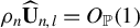
and proceeding as in the proof of (4.2), it can be shown that
$\rho _n\widehat {\mathbf {U}}_{n,l} = O_{\mathbb {P}}(1)$
 . Because
$\boldsymbol {\Gamma }_0$
 is positive definite and because
$\mathbf {t} \mapsto \widehat {M}_n(\boldsymbol {\theta }_{n,l}+\mathbf {t} \rho _n^{-1};h_{n,l})$
 is convex (almost surely), the corollary following Hjort and Pollard (Reference Hjort and Pollard1993, Lemma 2) implies that (4.1) holds.
4.3 Proof of Theorem 3
The proof of Theorem 3 is a natural bootstrap analog of the proof of Theorem 2.
For
$l \in \{0,\dots ,L\}$
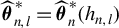
 , let
$\widehat {\boldsymbol {\theta }}^{\hspace{0.5pt}*}_{n,l}=\widehat {\boldsymbol {\theta }}^{\hspace{0.5pt}*}_n(h_{n,l})$
 and

where
$\mathbb {E}^{\hspace{0.5pt}*}_n[\cdot ]$
 denotes
$\mathbb {E}[\cdot |\mathbf {z}_1,\dots ,\mathbf {z}_n]$
 .
It suffices to show that

and that

where

For every
$\mathbf {t} \in \mathbb {R}^k$
 , using a Hoeffding decomposition and the fact that
$m(\mathbf {z},\mathbf {z};\boldsymbol {\theta }_{n,l})=0$
 and
$\mathbf {s}(\mathbf {z},\mathbf {z};\boldsymbol {\theta }_{n,l})=\mathbf {0}$
 for large n, we have

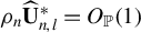
where it can be shown that
$\rho _n\widehat {\mathbf {U}}^{\hspace{0.5pt}*}_{n,l}=O_{\mathbb {P}}(1)$
 and where it follows from the proof of (4.1) that

where
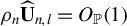
$\rho _n\widehat {\mathbf {U}}_{n,l}=O_{\mathbb {P}}(1)$
 . In other words,

Because
$\boldsymbol {\Gamma }_0$
 is positive definite and because
$\mathbf {t} \mapsto \widehat {M}^{\hspace{0.5pt}*}_n(\boldsymbol {\theta }_{n,l}+\mathbf {t} \rho _n^{-1};h_{n,l})$
 is convex (almost surely), the corollary following Hjort and Pollard (Reference Hjort and Pollard1993, Lemma 2) implies that (4.3) holds.
To prove (4.4), we begin by decomposing
$\widetilde {\mathbf {U}}^{\hspace{0.5pt}*}_n$
 as

where

and

Defining

routine calculations can be used to show that for every
$\boldsymbol {\mu }_1,\boldsymbol {\mu }_2 \in \mathbb {R}^k$
 , we have


and

where
$\mathbb {V}^{\hspace{0.5pt}*}_n[\cdot ]$
 denotes
$\mathbb {V}[\cdot |\mathbf {z}_1,\dots ,\mathbf {z}_n]$
 and

The Cramér–Wold device and the central limit theorem of Heyde and Brown (Reference Heyde and Brown1970) therefore imply that if
$\pi _n \to \pi _0 \in [0,1]$
 , then

Whether or not
$\pi _n$
 is convergent, the result (4.4) can be obtained from the preceding display by arguing along subsequences (if necessary).
4.4 Verifying Assumption 3
It follows from Lemma 1 that if Assumption 1 holds, then so does Assumption 3 with
$\mathtt {S}=0$
 . This observation provides the base case for an induction argument. To describe the induction step, suppose that for some even
$S \geq 0$
 , we have

Suppose also that, for every
$\mathbf {t} \in \mathbb {R}^k$
 and some
$\boldsymbol {\beta }_{S+2} \in \mathbb {R}^k$
 , we have

Then, the corollary following Hjort and Pollard (Reference Hjort and Pollard1993, Lemma 2) implies that

that is, defining
$\mathbf {b}_{S+2} = - \boldsymbol {\Gamma }_0^{-1} \boldsymbol {\beta }_{S+2}$
 , we have

To complete the proof of Proposition 1, it therefore suffices to note that (for every
$\mathbf {t} \in \mathbb {R}^k$
 and) under the assumptions of the proposition, we have

where

Similarly, if, in addition to the assumptions of Proposition 1, it is assumed that for every
$\mathbf {t} \in \mathbb {R}^k$
 and for some
$\boldsymbol {\beta }_4 \in \mathbb {R}^k$
 , we have

then Assumption 3 holds with
$\mathtt {S}=4$
 . One set of sufficient conditions for this to occur is that Assumptions 1 and 2 hold and that, for every
$\mathbf {t} \in \mathbb {R}^k$
 , the following are satisfied (with probability one):
-
(i) $\int _{\mathbb {R}^d} \|\mathbf {u}\|^4 K(\mathbf {u})d\mathbf {u}<\infty $
. -
(ii) $\bar {\mathbf {w}} \mapsto \boldsymbol {\varphi }(\mathbf {w},\bar {\mathbf {w}}) = \mathbb {E}[\mathbf {s}(\mathbf {z}_1,\mathbf {z}_2;\boldsymbol {\theta }_0)|\mathbf {w}_1=\mathbf {w},\mathbf {w}_2=\bar {\mathbf {w}}]f_{\mathbf {w}}(\bar {\mathbf {w}})$
is four times continuously differentiable with
$\mathbb {E}[\sup _{\bar {\mathbf {w}}\in \mathcal {W}}\|\partial _{\bar {\mathbf {w}}}^{\boldsymbol {\nu }} \boldsymbol {\varphi }(\mathbf {w},\bar {\mathbf {w}})\|]<\infty $
for all
$\boldsymbol {\nu }\in \mathbb {Z}_+^d$
with
$|\boldsymbol {\nu }|\leq 4$
. -
(iii) $f_{\mathbf {w}}$
is twice continuously differentiable and
$\bar {\mathbf {w}} \mapsto \mathbf {H}(\mathbf {w},\bar {\mathbf {w}};\boldsymbol {\theta }_0,\mathbf {t})$
is twice continuously differentiable with
$\mathbb {E}[\sup _{\bar {\mathbf {w}}\in \mathcal {W}}\|\partial _{\bar {\mathbf {w}}}^{\boldsymbol {\nu }} \mathbf {H}(\mathbf {w},\bar {\mathbf {w}};\boldsymbol {\theta }_0,\mathbf {t})f_{\mathbf {w}}(\bar {\mathbf {w}})\|]<\infty $
for all
$\boldsymbol {\nu }\in \mathbb {Z}_+^d$
with
$|\boldsymbol {\nu }|\leq 2$
. -
(iv) For some function $\dot {\mathbf {H}}(\mathbf {w},\bar {\mathbf {w}};\boldsymbol {\theta },\mathbf {t})\in \mathbb {R}^{k\times k}$
,
$\bar {\mathbf {w}} \mapsto \dot {\mathbf {H}}(\mathbf {w},\bar {\mathbf {w}};\boldsymbol {\theta }_0,\mathbf {t})$
is continuous, $$ \begin{align*} \mathbb{E}\left[\sup_{\bar{\mathbf{w}}\in\mathcal{W}}\|\dot{\mathbf{H}}(\mathbf{w},\bar{\mathbf{w}};\boldsymbol{\theta}_0,\mathbf{t})f_{\mathbf{w}}(\bar{\mathbf{w}})\|\right]<\infty, \end{align*} $$
$$ \begin{align*} \lim_{\tau\downarrow 0,(\boldsymbol{\theta},\mathbf{u})\to(\boldsymbol{\theta}_0,\mathbf{0})} \left\| \frac{\mathbf{H}(\mathbf{w},\mathbf{w}+\mathbf{u};\boldsymbol{\theta}+\tau\mathbf{t},\mathbf{t})-\mathbf{H}(\mathbf{w},\mathbf{w}+\mathbf{u};\boldsymbol{\theta},\mathbf{t})}{\tau}-\dot{\mathbf{H}}(\mathbf{w},\mathbf{w}+\mathbf{u};\boldsymbol{\theta},\mathbf{t}) \right\| = 0, \end{align*} $$and, for some $\delta>0$
, $$ \begin{align*} & \mathbb{E} \!\left[\! \sup_{ \tau\in (0,\delta),\|\boldsymbol{\theta}-\boldsymbol{\theta}_0\|<\delta, \mathbf{w}_2 \in\mathcal{W}} \!\left\| \!\frac{\mathbf{H}(\mathbf{w}_1,\mathbf{w}_2;\boldsymbol{\theta}+\tau\mathbf{t},\mathbf{t})-\mathbf{H}(\mathbf{w}_1,\mathbf{w}_2;\boldsymbol{\theta},\mathbf{t})}{\tau}-\dot{\mathbf{H}}(\mathbf{w}_1,\mathbf{w}_2;\boldsymbol{\theta},\mathbf{t}) \!\right\| \!\right]\\ & < \infty. \end{align*} $$













5 SUFFICIENT CONDITIONS FOR MOTIVATING EXAMPLES
To demonstrate the plausibility of Assumptions 1 and 2, we revisit the examples of Section 2. In each example, Assumption 1(ii) holds and Assumption 1(iii) is fairly primitive, so we focus on giving primitive sufficient conditions for Assumptions 1(iv), 1(v), and 2.
5.1 Partially Linear Regression Model
We take
$\mathbf {s}=\mathbf {s}_{\mathtt {PLR}}$
 and
$\mathbf {H}=\mathbf {H}_{\mathtt {PLR}}$
 , where

and

the latter depending on neither
$\boldsymbol {\theta }$
 nor
$\mathbf {t}$
 (because
$m_{\mathtt {PLR}}(\mathbf {z}_i,\mathbf {z}_j;\boldsymbol {\theta })$
 is quadratic in
$\boldsymbol {\theta }$
 ).
Under mild conditions, Assumptions 1(iv), 1(v), and 2 hold with


and

For instance, it suffices to set
$b(\mathbf {z}) = (1+\|\mathbf {x}\|) (1+\|\mathbf {x}\|+|\gamma _0(\mathbf {w})|+|\varepsilon |)$
 and to assume that
-
(i) The functions $\mathbf {w}\mapsto \gamma _0(\mathbf {w})$
,
$\mathbf {w}\mapsto \mathbb {E}[\mathbf {x}|\mathbf {w}]$
,
$\mathbf {w}\mapsto \mathbb {E}[\mathbf {x}\mathbf {x}'|\mathbf {w}]$
,
$\mathbf {w}\mapsto \mathbb {E}[\varepsilon ^2|\mathbf {w}]$
,
$\mathbf {w}\mapsto \mathbb {E}[\mathbf {x}\varepsilon ^2|\mathbf {w}]$
, and
$\mathbf {w}\mapsto \mathbb {E}[\mathbf {x}\mathbf {x}'\varepsilon ^2|\mathbf {w}]$
are continuous on
$\mathcal {W}$
. -
(ii) $\mathbb {E}[(1+\|\mathbf {x}\|^4)\varepsilon ^4] + \sup _{\mathbf {w}\in \mathcal {W}}\mathbb {E}[(1+\|\mathbf {x}\|^4)\varepsilon ^4 |\mathbf {w} ] f_{\mathbf {w}}(\mathbf {w})<\infty $
and $$ \begin{align*} \mathbb{E}[(1 \!+\! \|\mathbf{x}\|^4)\gamma_0(\mathbf{w})^4 \!+\! \|\mathbf{x}\|^8] \!+\! \sup_{\mathbf{w}\in\mathcal{W}}\mathbb{E}[(1+\|\mathbf{x}\|^4)\gamma_0(\mathbf{w})^4 \!+\! \|\mathbf{x}\|^8|\mathbf{w}]f_{\mathbf{w}}(\mathbf{w})\! < \!\infty. \end{align*} $$
-
(iii) With probability one, $\mathbb {V}[\mathbf {x}|\mathbf {w}]$
is positive definite and
$\mathbb {V}[\varepsilon |\mathbf {x},\mathbf {w}]>0$
.











Under the additional assumptions of Theorem 1 and if
$nh_n^d \to \infty $
 , the pairwise difference estimator is asymptotically linear with influence function

Unless the distribution of
$\mathbf {w}$
 is uniform on
$\mathcal {W}$
 , the pairwise difference estimator is therefore asymptotically distinct from the estimators studied by Robinson (Reference Robinson1988) and Donald and Newey (Reference Donald and Newey1994), the influence function of these estimators being given by

When
$nh_n^d \to 2c<\infty $
 , the pairwise difference estimator is still
$\sqrt {n}$
 -normal, but it ceases to be asymptotically linear. Similarly, the estimator of Donald and Newey (Reference Donald and Newey1994) is
$\sqrt {n}$
 -normal, but not asymptotically linear, when the associated tuning parameter is chosen appropriately (Cattaneo et al., Reference Cattaneo, Jansson and Newey2018), and in light of Linton (Reference Linton1995), it stands to reason that the same is true for the estimator of Robinson (Reference Robinson1988). Another
$\sqrt {n}$
 -normal estimator that is not asymptotically linear was proposed by Yatchew (Reference Yatchew1997). However, even under simplifying assumptions (e.g., uniformity of the distribution of
$\mathbf {w}$
 and/or conditional homoskedasticity of
$\varepsilon $
 ), it appears difficult to make insightful comparisons between the various estimators just mentioned.
5.2 Partially Linear Logit Model
We take
$\mathbf {s}=\mathbf {s}_{\mathtt {PLL}}$
 and
$\mathbf {H}=\mathbf {H}_{\mathtt {PLL}}$
 , where

and, defining
$\lambda (u) = \partial \Lambda (u)/\partial u = \exp (u)/[1+\exp (u)]^2$
 ,

where the latter does not depend on
$\mathbf {t}$
 (because
$m_{\mathtt {PLL}}(\mathbf {z}_i,\mathbf {z}_j;\boldsymbol {\theta })$
 is twice differentiable in
$\boldsymbol {\theta }$
 ).
Under mild conditions, Assumptions 1(iv), 1(v), and 2 hold with


and

For instance, it suffices to set
$b(\mathbf {z}) = 1+\|\mathbf {x}\|$
 and to assume that, for some
$\delta>0$
 ,
-
(i) The function $\mathbf {w}\mapsto \gamma _0(\mathbf {w})$
is continuous on
$\mathcal {W}$
. Also, the conditional distribution of
$\mathbf {x}$
given
$\mathbf {w}$
admits a density
$f_{\mathbf {x}|\mathbf {w}}$
with respect to some measure
$\rho $
such that
$\mathbf {w}\mapsto f_{\mathbf {x}|\mathbf {w}}(\mathbf {x}|\mathbf {w})$
is continuous on
$\mathcal {W}$
(with probability one) and $$ \begin{align*} \int_{\mathbb{R}^k} (1+ \|\mathbf{x}\|^2) \sup_{\|\mathbf{u}\|\leq\delta} f_{\mathbf{x}|\mathbf{w}}(\mathbf{x}| \mathbf{w} + \mathbf{u})d\rho(\mathbf{x})<\infty \qquad \text{for every } \mathbf{w}\in\mathcal{W}. \end{align*} $$
-
(ii) $\mathbb {E}[\|\mathbf {x}\|^4] + \sup _{\mathbf {w}\in \mathcal {W}}\mathbb {E}[\|\mathbf {x}\|^4 |\mathbf {w}]f_{\mathbf {w}}(\mathbf {w})<\infty .$
-
(iii) With probability one, $\mathbb {V}[\mathbf {x}|\mathbf {w}]$
is positive definite.







5.3 Partially Linear Tobit Model
We take
$\mathbf {s}=\mathbf {s}_{\mathtt {PLT}}$
 and
$\mathbf {H}=\mathbf {H}_{\mathtt {PLT}}$
 , where

and

with

Under mild conditions, Assumptions 1(iv), 1(v), and 2 hold with


and

For instance, it suffices to set
$b(\mathbf {z}) = 1+\|\mathbf {x}\|$
 and to assume that, for some
$\delta>0$
 ,
-
(i) The function $\mathbf {w}\mapsto \gamma _0(\mathbf {w})$
is continuous on
$\mathcal {W}$
. Also, the conditional distribution of
$\mathbf {x}$
given
$\mathbf {w}$
admits a density
$f_{\mathbf {x}|\mathbf {w}}$
with respect to some measure
$\rho $
such that
$\mathbf {w}\mapsto f_{\mathbf {x}|\mathbf {w}}(\mathbf {x}|\mathbf {w})$
is continuous on
$\mathcal {W}$
(with probability one) and $$ \begin{align*} \int_{\mathbb{R}^k} (1+ \|\mathbf{x}\|^2) \sup_{\|\mathbf{u}\|\leq\delta} f_{\mathbf{x}|\mathbf{w}}(\mathbf{x}| \mathbf{w} + \mathbf{u})d\rho(\mathbf{x})<\infty \qquad \text{for every } \mathbf{w}\in\mathcal{W}. \end{align*} $$
In addition, the function $(\varepsilon ,\mathbf {w})\mapsto f_{\varepsilon |\mathbf {w}}(\varepsilon |\mathbf {w})$
is continuous and bounded and the function $$ \begin{align*} (\mathbf{x},\mathbf{w})\mapsto \int_{\mathbb{R}} \sup_{|u|+\|\mathbf{u}\|\leq\delta}f_{\varepsilon|\mathbf{w}}(\varepsilon-\mathbf{x}'\boldsymbol{\theta}_0-\gamma_0(\mathbf{w})+u|\mathbf{w}+\mathbf{u})d\varepsilon \end{align*} $$is bounded.
-
(ii) $\mathbb {E}[\|\mathbf {x}\|^4] + \sup _{\mathbf {w}\in \mathcal {W}}(1+\mathbb {E}[\|\mathbf {x}\|^4 |\mathbf {w}])f_{\mathbf {w}}(\mathbf {w})<\infty .$
-
(iii) With probability one, $\mathbb {V}[\mathbf {x}|\mathbf {w}]$
is positive definite.









6 SIMULATION EVIDENCE
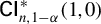
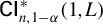
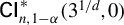
We present simulation evidence for the partially linear regression and partially linear logit models. We compare the four bootstrap-based confidence intervals discussed in Section 3.5:
$\mathsf {CI}_{n,1-\alpha }^{\hspace{0.5pt}*}(1,0)$
 ,
$\mathsf {CI}_{n,1-\alpha }^{\hspace{0.5pt}*}(1,L)$
 ,
$\mathsf {CI}_{n,1-\alpha }^{\hspace{0.5pt}*}(3^{1/d},0)$
 , and
$\mathsf {CI}_{n,1-\alpha }^{\hspace{0.5pt}*}(3^{1/d},L)$
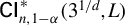 . We set
$\alpha =0.05$
 , and for the debiasing procedure, we use
$L=1$
 and
$\mathbf {c}=(1,2)'$
 .
6.1 Simulation Design: Partially Linear Regression Model
We base the partially linear regression designs on equations (6.1) and (6.2) of Robinson (Reference Robinson1988). We consider

The three designs are as follows. In Model 1,
$x_i=2v_i$
 ,
$v_i\sim \mathsf {N}(0,1)$
 ,
$w_i=v_i+u_i$
 ,
$u_i\sim \mathrm {N}(0,2)$
 ,
$\gamma _0(w)=w^2+1$
 ,
$\varepsilon _i\sim \mathsf {N}(0,1)$
 , and
$\{v_i,u_i,\varepsilon _i\}$
 are jointly independent. In Model 2,
$d=\dim (\mathbf {w})=2$
 ,
$\gamma _0(\mathbf {w})=\mathbf {w}'\mathbf {w}+1$
 ,
$(x_i,\mathbf {w}_i')'$
 is normal with each component having mean
$1$
 and variance
$3$
 , and any pair in
$(x_i,\mathbf {w}_i')'$
 has correlation
$2/3$
 . Model 3 uses the same joint normal specification for
$(x_i,\mathbf {w}_i')'$
 as Model 2, but with
$d=\dim (\mathbf {w})=3$
 . In all models,
$\theta _0=1$
 . The regressor of interest
$x_i$
 is correlated with
$\mathbf {w}_i$
 , and thus, ignoring the
$\gamma _0(\mathbf {w}_i)$
 term will induce bias in the estimator of
$\theta _0$
 .
6.2 Simulation Design: Partially Linear Logit Model
We base the partially linear logit designs on those of Honoré and Powell (Reference Honoré, Powell, Andrews and Stock2005). As in the partially linear regression simulations, the three designs differ mainly in the dimension of
$\mathbf {w}$
 . We consider

where the CDF of
$\varepsilon _i$
 is
$\Lambda , x_{2i}$
 has a discrete distribution with
$\mathbb {P}[x_{2i}=1]=1/2=\mathbb {P}[x_{2i}=-1]$
 ,
$x_{1i}=v_i + \mathbf {w}_i'\mathbf {w}_i$
 with
$v_i\sim \mathsf {N}(0,1)$
 , and
$\{\varepsilon _i,\mathbf {w}_i,x_{2i},v_i\}$
 are jointly independent. For Model d (
$d\in \{1,2,3\}$
 ),
$\dim (\mathbf {w})=d$
 , and
$\mathbf {w}_i$
 has a normal distribution with each element having mean zero and variance one, equicorrelated with correlation
$0.2$
 . In all models,
$\boldsymbol {\theta }_0=(1, 1)'$
 .
As noted by Honoré and Powell (Reference Honoré, Powell, Andrews and Stock2005), ignoring the presence of
$\gamma _0(\mathbf {w}_i)$
 induces bias in the estimator of
$\boldsymbol {\theta }_0$
 , although the bias for the second element tends to be negligible relative to the standard error. We focus on constructing
$95\%$
 confidence intervals for the first element of
$\boldsymbol {\theta }_0$
 .
6.3 Simulation Results
Tables 1–3 display the coverage probabilities and average lengths of the four confidence intervals for the partially linear regression model, and Tables 4–6 for the partially linear logit model. Figure 2 complements the tables by plotting coverage probability as a function of bandwidth h for all six DGPs. For each data-generating process, the sample size was
$n=2{,}000$
 , we conducted
$2{,}000$
 simulation replications, and for each replication, we drew
$2{,}000$
 bootstrap samples to compute bootstrap quantiles.
Bootstrap 95% confidence intervals for partially linear regression model: DGP 1 (
$d=1$
 ).

Table 1 Long description
The table is structured with a primary header row dividing the data into two main groups: B equals 1 and B equals 3 super 1 all over d. Under each of these, a secondary header divides the data by L equals 0 and L equals 1. Each of these four sub-sections contains two columns: Coverage and Length.
The first column, h, lists bandwidth values from 0.35 to 1.50.
Key data trends:
* For B equals 1, Coverage remains stable near 0.95 across all h values for both L equals 0 and L equals 1, with Length staying constant at approximately 0.058 to 0.060.
* For B equals 3 super 1 all over d, Coverage and Length increase significantly as h increases. For L equals 0, Coverage starts at 0.956 at h equals 0.35 and reaches 1.000 by h equals 1.10, while Length grows from 0.058 to 0.119.
* For L equals 1 in the second group, Coverage starts at 0.956 and reaches 1.000 at h equals 1.30, with Length growing from 0.058 to 0.108.
Specific rows are highlighted: h equals 0.70 is highlighted in yellow, and h equals 1.00 is highlighted in orange, representing M S E-optimal bandwidths for L equals 0 and L equals 1 respectively.
Note: The table shows coverage probability and average length of confidence intervals over
$2{,}000$
 simulation replications. The sample size is
$n=2{,}000$
 and the number of bootstrap draws is
$2{,}000$
 . The rows highlighted in yellow and orange correspond to the estimated MSE-optimal bandwidths for the point estimators with
$L=0$
 and
$L=1$
 , respectively.
Bootstrap 95% confidence intervals for partially linear regression model: DGP 2 (
$d=2$
 ).
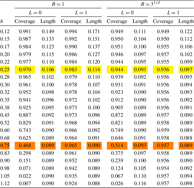
Table 2 Long description
The table is structured with a primary column for bandwidth h and two main super-columns for B = 1 and B = 3 super 1/d. Each super-column is subdivided into L = 0 and L = 1, which are further split into Coverage and Length metrics.
* Headers: The first column is h. The next four columns fall under B = 1 (subdivided into L = 0 and L = 1). The final four columns fall under B = 3 super 1/d (subdivided into L = 0 and L = 1).
* Data Trends: As h increases from 0.12 to 1.12:
* For B = 1, L = 0: Coverage drops significantly from 0.991 to 0.007, while Length decreases from 0.149 to 0.090.
* For B = 1, L = 1: Coverage remains relatively stable, starting at 0.994 and ending at 0.924, with Length decreasing from 0.171 to 0.088.
* For B = 3 super 1/d, L = 0: Coverage drops from 0.949 to 0.026, while Length stays relatively flat around 0.090 to 0.116.
* For B = 3 super 1/d, L = 1: Coverage remains very stable between 0.949 and 0.957, with Length decreasing from 0.122 to 0.098.
* Specific Values: At h = 0.30, Coverage for B = 1, L = 0 is 0.961 and for L = 1 is 0.978. For B = 3 super 1/d, L = 0 is 0.931 and L = 1 is 0.956.
Note: The table shows coverage probability and average length of confidence intervals over
$2{,}000$
 simulation replications. The sample size is
$n=2{,}000$
 and the number of bootstrap draws is
$2{,}000$
 . The rows highlighted in yellow and orange correspond to the estimated MSE-optimal bandwidths for the point estimators with
$L=0$
 and
$L=1$
 , respectively.
Bootstrap 95% confidence intervals for partially linear regression model: DGP 3 (
$d=3$
 ).
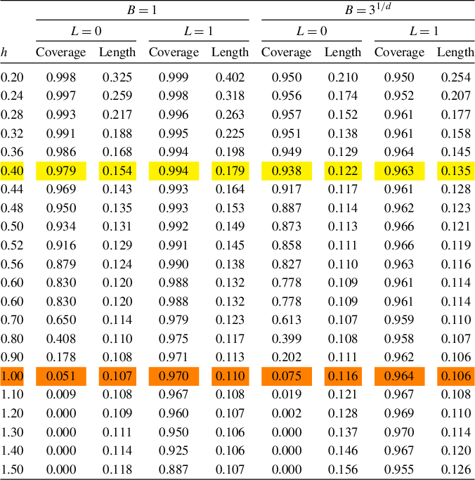
Table 3 Long description
The table displays Coverage and Length metrics for two primary groups: B = 1 and B = 3 super 1/d. Each group is further subdivided into L = 0 and L = 1.
* Header Structure: The first column is h (bandwidth). The subsequent columns are paired as Coverage and Length for the following four conditions:
1. B = 1, L = 0
2. B = 1, L = 1
3. B = 3 super 1/d, L = 0
4. B = 3 super 1/d, L = 1
* Data Trends:
As h increases from 0.20 to 1.50:
- For B = 1, L = 0: Coverage drops sharply from 0.998 to 0.000, while Length decreases from 0.325 to 0.118.
- For B = 1, L = 1: Coverage remains high (above 0.950) until h = 1.40, where it begins to decline to 0.887.
- For B = 3 super 1/d, L = 0: Coverage drops from 0.950 to 0.000, with Length decreasing from 0.210 to 0.156.
- For B = 3 super 1/d, L = 1: Coverage remains stable and high, ranging between 0.950 and 0.970 across all values of h, while Length decreases from 0.254 to 0.126.
Row h = 0.40 is highlighted in yellow, and row h = 1.00 is highlighted in orange, representing M S E-optimal bandwidths for L = 0 and L = 1 respectively.
Note: The table shows coverage probability and average length of confidence intervals over
$2{,}000$
 simulation replications. The sample size is
$n=2{,}000$
 and the number of bootstrap draws is
$2{,}000$
 . The rows highlighted in yellow and orange correspond to the estimated MSE-optimal bandwidths for the point estimators with
$L=0$
 and
$L=1$
 , respectively.
Bootstrap 95% confidence intervals for partially linear logit model: DGP 1 (
$d=1$
 ).
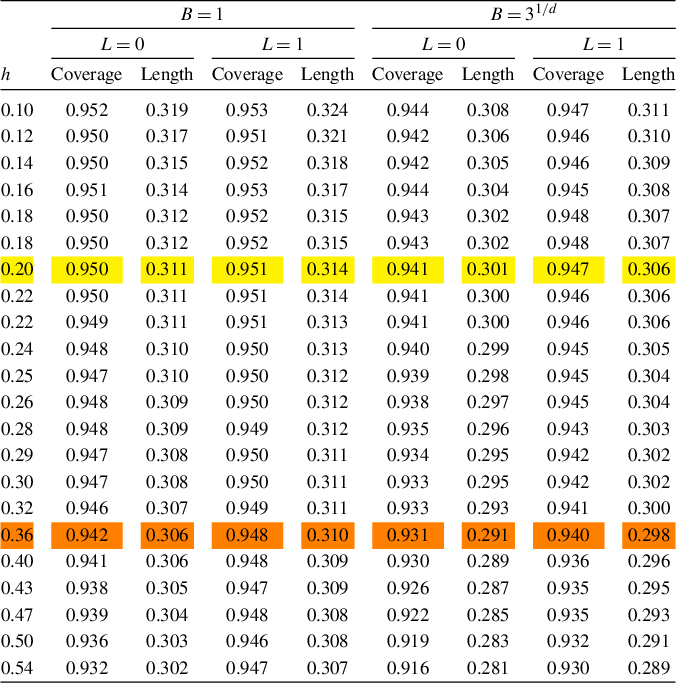
Table 4 Long description
The table presents Coverage and Length metrics for two main scenarios: B equals 1 and B equals 3 super 1/d. Each scenario is further divided into L equals 0 and L equals 1.
* Column Structure: The first column is h (bandwidth). The subsequent columns are paired as Coverage and Length for each combination of B and L.
* Data Trends: As h increases from 0.10 to 0.54, the Length of the confidence intervals generally decreases across all categories. For example, at B equals 1 and L equals 0, Length drops from 0.319 to 0.302. Coverage remains relatively stable near 0.95 for lower h values but shows a slight decline as h increases, particularly in the B equals 3 super 1/d and L equals 0 category, which drops to 0.916 at h equals 0.54.
* Specific Highlights:
- Row h equals 0.20 is highlighted in yellow, representing the M S E-optimal bandwidth for L equals 0, with coverage values of 0.950 and 0.943.
- Row h equals 0.36 is highlighted in orange, representing the M S E-optimal bandwidth for L equals 1, with coverage values of 0.951 and 0.946.
* Simulation Parameters: Based on 2,000 replications with a sample size n equals 2,000 and 2,000 bootstrap draws.
Note: The table shows coverage probability and average length of confidence intervals over
$2{,}000$
 simulation replications. The sample size is
$n=2{,}000$
 and the number of bootstrap draws is
$2{,}000$
 . The rows highlighted in yellow and orange correspond to the estimated MSE-optimal bandwidths for the point estimators with
$L=0$
 and
$L=1$
 , respectively.
Bootstrap 95% confidence intervals for partially linear logit model: DGP 2 (
$d=2$
 ).
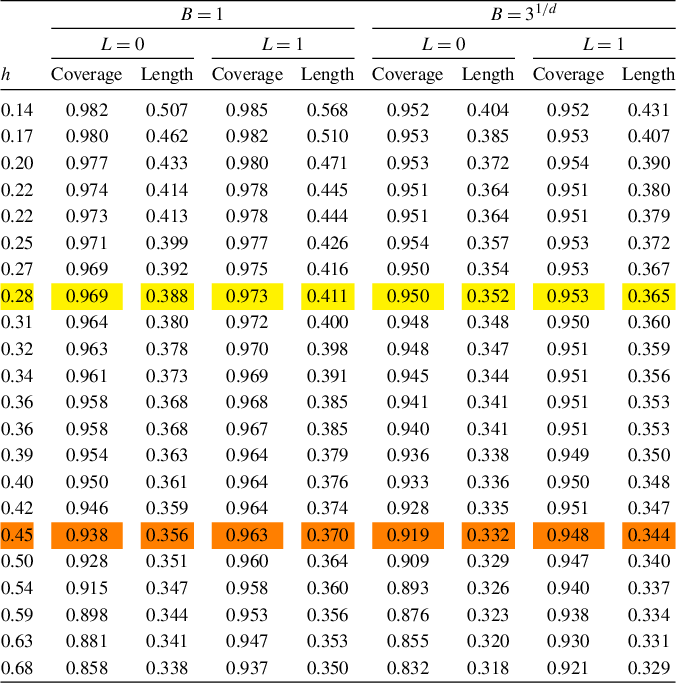
Table 5 Long description
The table is structured with a primary header row dividing the data into two main groups: B = 1 and B = 3 super 1/d. Below these, a secondary header divides each group by L = 0 and L = 1. Each of these four sub-sections contains two columns: Coverage and Length.
The leftmost column is h, representing bandwidth, with 22 rows ranging from 0.14 to 0.68.
Key data trends:
* For B = 1 and L = 0: As h increases from 0.14 to 0.68, Coverage decreases from 0.982 to 0.858, and Length decreases from 0.507 to 0.338.
* For B = 1 and L = 1: Coverage decreases from 0.985 to 0.937, and Length decreases from 0.568 to 0.350.
* For B = 3 super 1/d and L = 0: Coverage decreases from 0.952 to 0.832, and Length decreases from 0.404 to 0.318.
* For B = 3 super 1/d and L = 1: Coverage remains relatively stable, starting at 0.952 and ending at 0.921, while Length decreases from 0.431 to 0.329.
Specific rows are highlighted: h = 0.22 and h = 0.36 are highlighted in yellow (corresponding to M S E-optimal bandwidths for L = 0), and h = 0.28 and h = 0.45 are highlighted in orange (corresponding to M S E-optimal bandwidths for L = 1).
Note: The table shows coverage probability and average length of confidence intervals over
$2{,}000$
 simulation replications. The sample size is
$n=2{,}000$
 and the number of bootstrap draws is
$2{,}000$
 . The rows highlighted in yellow and orange correspond to the estimated MSE-optimal bandwidths for the point estimators with
$L=0$
 and
$L=1$
 , respectively.
Bootstrap 95% confidence intervals for partially linear logit model: DGP 3 (
$d=3$
 ).
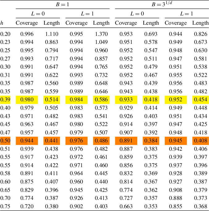
Table 6 Long description
The table is structured with a primary header row for B = 1 and B = 3 super 1 all over d. Under each B value, there are sub-headers for L = 0 and L = 1. Each of these four categories contains two columns: Coverage and Length. The leftmost column is the bandwidth h, ranging from 0.20 to 0.75.
Key data trends include:
* For B = 1, L = 0: Coverage starts at 0.996 at h = 0.20 and decreases to 0.720 at h = 0.75. Length decreases from 1.110 to 0.380.
* For B = 1, L = 1: Coverage starts at 0.995 and decreases to 0.902. Length decreases from 1.370 to 0.403.
* For B = 3 super 1 all over d, L = 0: Coverage starts at 0.953 and decreases to 0.663. Length decreases from 0.693 to 0.353.
* For B = 3 super 1 all over d, L = 1: Coverage starts at 0.944 and decreases to 0.855. Length decreases from 0.826 to 0.368.
Specific rows are highlighted: h = 0.39 is highlighted in yellow for L = 0 M S E-optimal bandwidths, and h = 0.50 is highlighted in orange for L = 1 M S E-optimal bandwidths.
Note: The table shows coverage probability and average length of confidence intervals over
$2{,}000$
 simulation replications. The sample size is
$n=2{,}000$
 and the number of bootstrap draws is
$2{,}000$
 . The rows highlighted in yellow and orange correspond to the estimated MSE-optimal bandwidths for the point estimators with
$L=0$
 and
$L=1$
 , respectively.
Coverage probabilities as a function of bandwidth h.
Note: Each panel plots the empirical coverage probability of
$\mathsf {CI}_{n,0.95}^{\hspace{0.5pt}*}(B,L)$
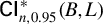 against bandwidth h for the four procedures
$(B,L)\in \{(1,0),(1,1),(3^{1/d},0),(3^{1/d},1)\}$
 . “PLR” stands for the partially linear regression model, and “PLL” stands for the partially linear logit model. d denotes the dimension of
$\mathbf {w}$
 . The horizontal dotted line marks the
$95\%$
 nominal level. The two vertical lines mark the estimated MSE-optimal bandwidths
$h_{L=0}$
 and
$h_{L=1}$
 for the point estimators
$\widehat {\boldsymbol {\theta }}_n$
 (
$L=0$
 ) and
$\widetilde {\boldsymbol {\theta }}_n$
 (
$L=1$
 ), respectively. The sample size is
$n=2{,}000$
 and results are based on
$2{,}000$
 simulation replications with
$2{,}000$
 bootstrap samples.
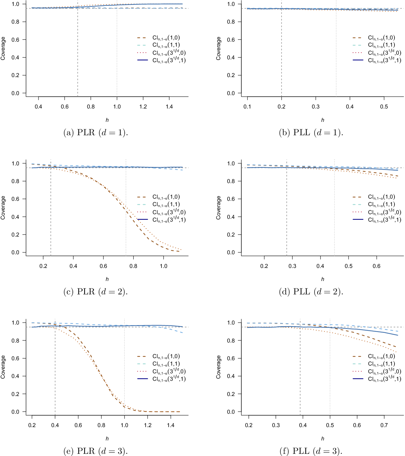
Figure 2 Long description
A multi-panel figure with six line graphs labeled a through f. Each graph plots Coverage on the y-axis from 0.0 to 1.0 against bandwidth h on the x-axis. A horizontal dotted line at 0.95 represents the nominal level. Two vertical dashed lines mark M S E-optimal bandwidths h sub L equals 0 and h sub L equals 1.
* Panel a, P L R d equals 1: All four lines remain stable near the 0.95 level across h from 0.4 to 1.4.
* Panel b, P L L d equals 1: All four lines are tightly clustered at the 0.95 level across h from 0.1 to 0.5.
* Panel c, P L R d equals 2: The lines for C I sub n, 1 minus alpha (1, 0) and (3 to the 1 over d power, 0) show a sharp sigmoidal decline from 0.95 toward 0.0 as h increases beyond 0.4. The other two lines remain stable.
* Panel d, P L L d equals 2: Similar to panel c, but the decline is much more gradual, staying above 0.8.
* Panel e, P L R d equals 3: The decline for the two sensitive lines is even steeper than in d equals 2, reaching 0.0 by h equals 1.2.
* Panel f, P L L d equals 3: The decline for the two sensitive lines is more pronounced than in d equals 2 but remains significantly higher than the P L R counterpart, ending near 0.7.
In all panels, the legend identifies four procedures: C I sub n, 1 minus alpha (1, 0) as a brown dashed line, (1, 1) as a light blue dashed line, (3 to the 1 over d power, 0) as a brown dotted line, and (3 to the 1 over d power, 1) as a solid dark blue line.
The panel headed “
$B=1$
 ” refers to
$\mathsf {CI}_{n,0.95}^{\hspace{0.5pt}*}(1,L)$
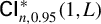 , in which the bandwidth used to compute bootstrapped quantiles equals the bandwidth used for estimation. The panel headed “
$B=3^{1/d}$
 ” refers to our proposed methods
$\mathsf {CI}_{n,0.95}^{\hspace{0.5pt}*}(3^{1/d},L)$
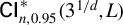 , in which the bandwidth for bootstrap estimation is rescaled by the factor
$3^{1/d}$
 . Within each panel,
$L=0$
 is based on the estimator
$\widehat {\boldsymbol {\theta }}_n$
 and
$L=1$
 is based on the debiased estimator
$\widetilde {\boldsymbol {\theta }}_n$
 with
$\mathbf {c}=(1, 2)'$
 .
To form the bandwidth grid, we first estimate
$h_{L=0}$
 and
$h_{L=1}$
 by auxiliary simulations. These are the MSE-minimizing bandwidths for
$\widehat {\boldsymbol {\theta }}_n$
 and
$\widetilde {\boldsymbol {\theta }}_n$
 , respectively. The grid is then taken as the union of
$h_{L=0}\times \{0.5,\dots ,1.5\}$
 and
$h_{L=1}\times \{0.5,\dots ,1.5\}$
 (increments of
$0.1$
 ). Rows highlighted in yellow and orange in the tables mark
$h_{L=0}$
 and
$h_{L=1}$
 , respectively.
The results are broadly consistent with our theoretical predictions. We focus on two forces of particular interest: small-bandwidth regions, where the standard bootstrap variance may be inflated, and large-bandwidth regions, where smoothing bias may become non-negligible. The simulations also include one instructive qualification: in the partially linear regression model with
$d=1$
 , the conventional procedures are already very well calibrated, while our proposed procedure
$\mathsf {CI}_{n,0.95}^{\hspace{0.5pt}*}(3^{1/d},1)$
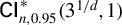 is conservative. This is a specialized design in which the smoothing bias targeted by jackknife debiasing is negligible, so bandwidth rescaling and debiasing mostly widen the intervals without offsetting a meaningful bias. This qualification is specific to the partially linear regression
$d=1$
 design and does not describe the partially linear logit model with
$d=1$
 , where uncorrected intervals exhibit undercoverage as the bandwidth grows and bias correction is beneficial.
6.3.1 Small-Bandwidth Overcoverage
For small bandwidths, the confidence intervals
$\mathsf {CI}_{n,0.95}^{\hspace{0.5pt}*}(1,L)$
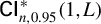 tend to overcover the nominal
$95\%$
 level, whereas our proposed methods
$\mathsf {CI}_{n,0.95}^{\hspace{0.5pt}*}(3^{1/d},L)$
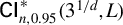 achieve coverage close to the nominal probability. This observation is predicted by our small-bandwidth asymptotics: using the same
$h_n$
 for both estimation and the bootstrap quantile computation causes the bootstrap to overestimate the sampling dispersion of
$\widehat {\boldsymbol {\theta }}_n$
 . The average interval lengths in the tables are in line with this prediction. At small bandwidths,
$\mathsf {CI}_{n,0.95}^{\hspace{0.5pt}*}(1,L)$
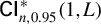 are systematically longer than their
$\mathsf {CI}_{n,0.95}^{\hspace{0.5pt}*}(3^{1/d},L)$
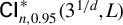 counterparts.
The severity of this distortion grows sharply with
$d=\dim (\mathbf {w})$
 , consistent with our theoretical prediction that the larger d, the wider the small-bandwidth region (based on the condition
$\liminf _{n\to \infty }nh_n^d<\infty $
 ). For the partially linear regression model with
$d=2$
 and
$d=3$
 , the coverage probabilities for
$\mathsf {CI}_{n,0.95}^{\hspace{0.5pt}*}(1,L)$
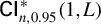 are well above the nominal level for smaller bandwidths, whereas our methods
$\mathsf {CI}_{n,0.95}^{\hspace{0.5pt}*}(3^{1/d},L)$
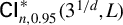 achieve the nominal level (Tables 2 and 3). The same small-bandwidth variance distortion is visible in the logit model. Overcoverage under
$\mathsf {CI}_{n,0.95}^{\hspace{0.5pt}*}(1,0)$
 is modest for
$d=1$
 , rises to
$0.982$
 for
$d=2$
 , and reaches
$0.996$
 for
$d=3$
 at the smallest bandwidth used in the simulation (Tables 4–6), with analogous patterns for
$\mathsf {CI}_{n,0.95}^{\hspace{0.5pt}*}(1,1)$
 . Figure 2 makes this dimension-dependence visually apparent: the coverage curves are well above the nominal level (the horizontal dotted line) for
$d>1$
 .
6.3.2 Large-Bandwidth Undercoverage and Bias Correction
At larger bandwidths, except in the partially linear regression
$d=1$
 design discussed above, the bias may become non-negligible, and
$\mathsf {CI}_{n,0.95}^{\hspace{0.5pt}*}(B,0)$
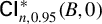 tends to exhibit severe undercoverage. For the partially linear regression model with
$d=2$
 , the coverage of
$\mathsf {CI}_{n,0.95}^{\hspace{0.5pt}*}(1,0)$
 falls to
$0.468$
 at
$h=0.75$
 and to
$0.007$
 at
$h=1.12$
 . For
$d=3$
 , it falls to
$0.051$
 at
$h=1.00$
 and to essentially zero for
$h\geq 1.20$
 . The undercoverage is similarly pronounced in the logit model: for
$d=2$
 , coverage collapses to
$0.858$
 at
$h=0.68$
 , and for
$d=3$
 , it falls to
$0.720$
 at
$h=0.75$
 .
The debiased intervals correct this distortion effectively. At larger bandwidths, the
$(B=1,L=1)$
 procedure is closer to the nominal
$95\%$
 level than the
$(B=1,L=0)$
 procedure: for the partially linear regression model with
$d=2$
 , coverage is
$0.965$
 at
$h_{L=1}=0.75$
 , and for
$d=3,$
 it is
$0.970$
 at
$h_{L=1}=1.00$
 . Similar patterns hold for the logit model, where coverage is
$0.963$
 at
$h_{L=1}=0.45$
 for
$d=2$
 and
$0.976$
 at
$h_{L=1}=0.50$
 for
$d=3$
 .
6.3.3 Combining Bandwidth Rescaling and Bias Correction
Under the procedure that combines bandwidth rescaling and bias correction,
$\mathsf {CI}_{n,0.95}^{\hspace{0.5pt}*}(3^{1/d},1)$
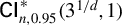 , coverage remains close to the nominal level across a wide bandwidth range. For the partially linear regression model with
$d=2$
 , the coverage probabilities lie between
$0.949$
 and
$0.959$
 across all bandwidths on the grid. For
$d=3$
 , coverage ranges from
$0.950$
 to
$0.970$
 over most of the grid and remains at
$0.955$
 even at
$h=1.50$
 . The cost of bias correction is a modest increase in average interval length relative to the uncorrected
$L=0$
 intervals: comparing the
$(B=3^{1/d},L=0)$
 and
$(B=3^{1/d},L=1)$
 columns at the MSE-optimal bandwidth
$h_{L=0}$
 , the debiased intervals are roughly
$4\%$
 wider for
$d=2$
 and roughly
$11\%$
 wider for
$d=3$
 in the partially linear regression model, a small price given the improvement in coverage reliability for larger bandwidths. For the logit model, the qualitative picture is the same for
$d=2$
 and
$d=3$
 . For
$d=1$
 , the proposed method is not conservative in the same way as in the partially linear regression case; instead, the main issue is the emergence of bias as the bandwidth grows, which bias correction partly offsets. Under the proposed procedure, coverage remains close to the nominal
$95\%$
 across a wide range of bandwidths considered.
Overall, the simulation evidence supports combining bandwidth rescaling (
$B=3^{1/d}$
 ) with jackknife-based bias correction (
$L=1$
 ), especially when smoothing bias is present or when the dimension of the nonparametric component is moderate. The partially linear regression
$d=1$
 design provides a useful reminder that when conventional methods are already well calibrated and the relevant smoothing bias is essentially absent, the robust procedure can be conservative.
7 CONCLUSION
This article develops bandwidth-robust distribution theory and bootstrap-based inference procedures for a broad class of convex pairwise difference estimators. Our theoretical work is based on small-bandwidth asymptotics and carefully leverages convexity. We illustrate the theory with three prominent examples. In addition to expanding the scope of small-bandwidth asymptotics, our results lay the groundwork for several promising avenues of future research. First, our methods could be generalized to develop bandwidth selection based on higher-order stochastic expansions. Second, consistent variance estimators could be developed as an alternative to bootstrap-based inference. Third, it would be of interest to expand our theory to allow for pairwise difference estimators based on generated regressors, a class of estimators that sometimes arises in the context of control function and related econometric methods. Finally, it seems plausible that there exist settings where the objective function is sufficiently non-smooth to result in non-Gaussian distributional approximations. We leave these extensions for future work.
FUNDING STATEMENT
M.D.C. gratefully acknowledges financial support from the National Science Foundation through grants SES-1947805, DMS-2210561, and SES-2241575. M.J. gratefully acknowledges financial support from the National Science Foundation through grant SES-1947662 and from the Aarhus Center for Econometrics (ACE), funded by the Danish National Research Foundation through grant DNRF186. K.N. gratefully acknowledges financial support from the British Academy through grant SRG24∖241614.
COMPETING INTEREST STATEMENT
The authors declare that no competing interests exist.
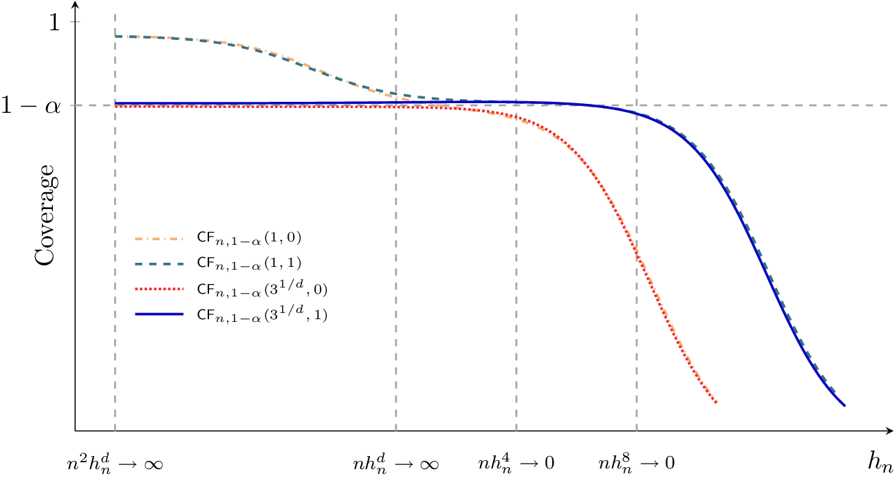
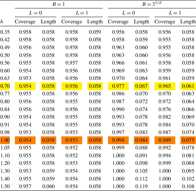

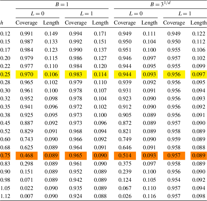

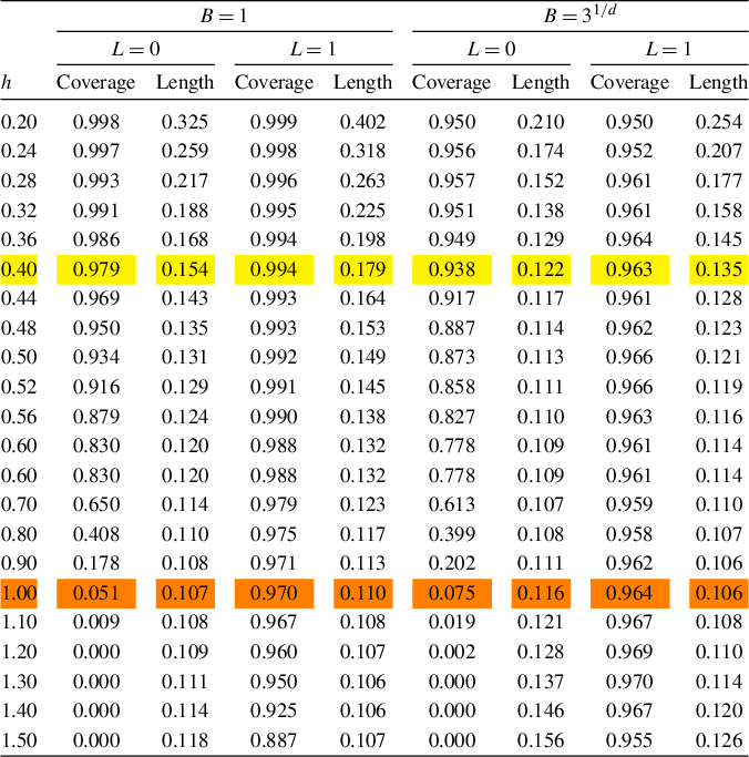

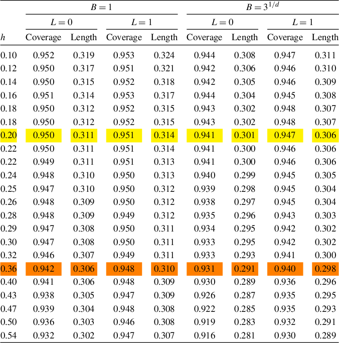

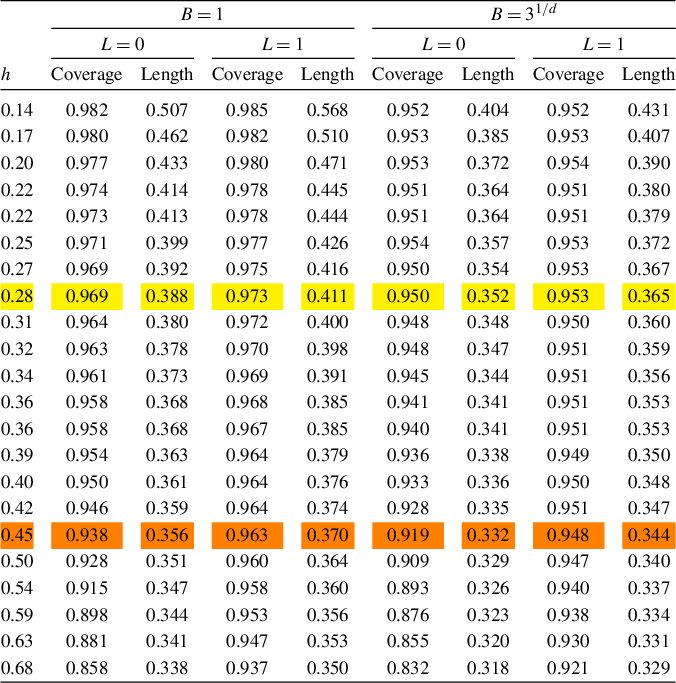

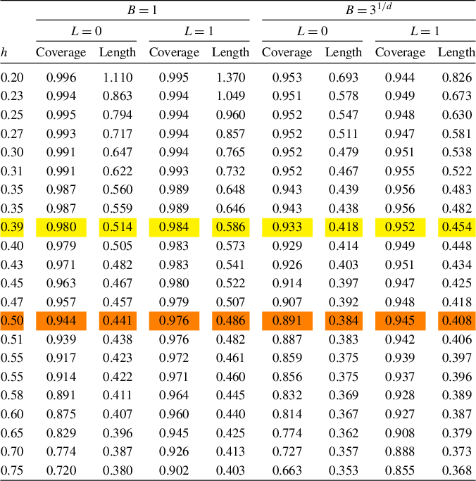

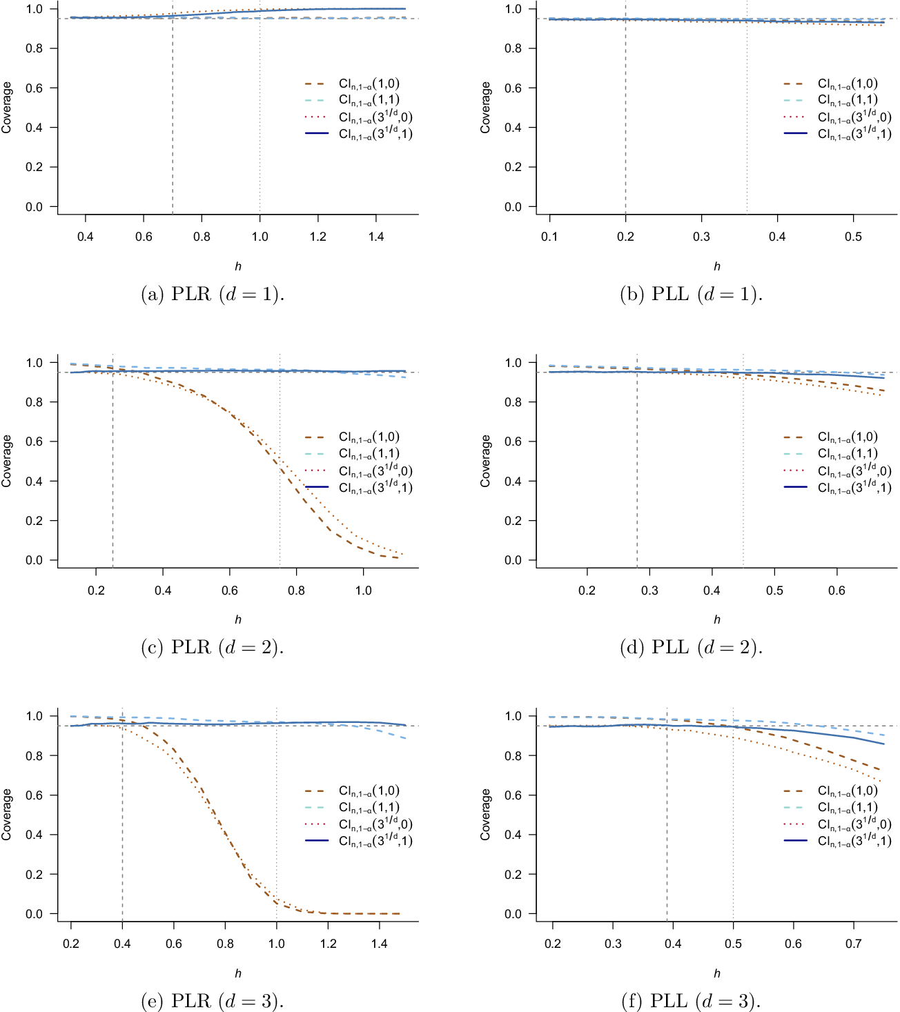


 Open access

