



1. Introduction
The prediction and control of the laminar–turbulent transition on swept wings begin with the characterisation of the attachment-line flow. Turbulent flow on the attachment line will be carried along the upper and lower surfaces of the wing resulting in a ‘fully turbulent’ state. A laminar attachment line enables a zone of laminar flow that reaches downstream from the wing leading edge – the extent of which will depend on subsequent instabilities or bypass mechanisms (e.g. Tollmien–Schlichting waves, cross-flow instabilities). Thus, for laminar flow control applications seeking to reduce drag, it is necessary to establish a laminar attachment line. If turbulent flow is desired for enhanced mixing or to delay separation, it is sufficient to establish a turbulent attachment line.
Surface heating effects can alter the state of the attachment line, potentially impacting the targeted downstream benefits of either laminar or turbulent flow. Recent studies aimed at incorporating hybrid-electric propulsion have demonstrated the need to efficiently offload significant levels of heat (Kellermann et al. Reference Kellermann, Habermann and Hornung2019). One approach to expelling the heat is to exploit convective cooling along the wing surface, but if this degrades laminar flow it can result in increasing drag (Barahona et al. Reference Barahona, van de Weijer, Vidales and Kotsonis2024).
In instances where turbulent flow is desired, attachment-line heating could prove beneficial. Reed & Saric (Reference Reed and Saric2014), for example, considered the use of leading-edge heating to trigger transition on a laminar-flow wing to provide better handling characteristics when needed. Avoiding surface overheating due to wing anti-ice operation during dry-air conditions is another application where turbulent flow is advantageous. These applications can result in large wall temperatures
 $T_w$
relative to the boundary-layer edge temperature
 $T_e$
or the free-stream temperature
 $T_{\infty }$
, with values of
 $T_w / T_e$
greater than 1.5. This motivates the need to better understand and predict the role of surface heating in determining the attachment-line state.
In subsonic flows, the attachment line can be characterised by a Reynolds number based on inviscid-flow quantities,
 $\bar R =W \delta _r / \nu$
, where
 $W$
is the edge velocity along the attachment line,
 $\nu$
is the kinematic viscosity and
 $\delta _r = \sqrt {\nu / ({\rm d}U/{\rm d}s)|_{s=0}}$
is an equilibrium boundary-layer thickness resulting from balancing viscous boundary-layer growth with the suppression of growth due to inviscid strain (where
 $s$
is the surface distance normal to the attachment line). The Reynolds number
 $\bar R$
can be related to the momentum-thickness Reynolds number
 $R_\theta =W \theta /\nu$
through the relationship
 $R_{\theta }^{\textit{Lam}} \approx 0.404 \bar R$
for a laminar attachment-line boundary layer. For a turbulent attachment line, this relationship is
 $R_{\theta }^{\textit{Turb}} \approx 1.64(\bar R-160)$
based on a line through the simulation results of Spalart (Reference Spalart1989) and the experimental results of Cumpsty & Head (Reference Cumpsty and Head1969).
The stability analysis of Hall et al. (Reference Hall, Malik and Poll1984) for an attachment line with an adiabatic wall boundary condition identified a critical
 $\bar R =583$
for onset of instability. This
 $\bar R$
value is consistent with experimental observations for the onset on natural transition near
 $\bar R \approx 600$
(Pfenninger & Bacon Jr Reference Pfenninger and Bacon1969; Poll Reference Poll1979). Direct numerical simulations of Spalart (Reference Spalart1989) and Joslin (Reference Joslin1995) also confirm
 $\bar R \approx 580$
for transition due to instability. Subsequent stability analyses considered other forms of perturbation that can also be unstable, but these occur at higher values of
 $\bar R$
(Lin & Malik Reference Lin and Malik1996; Theofilis et al. Reference Theofilis, Fedorov, Obrist and Dallmann2003). The analyses of Hall & Malik (Reference Hall and Malik1986) and Balakumar & Trivedi (Reference Balakumar and Trivedi1998) show the existence of finite-amplitude equilibrium states at subcritical
 $\bar R$
values down to
 $\bar R=511$
. These equilibrium states are unstable to three-dimensional disturbances, suggesting a path to transition if the attachment line is initialised with sufficiently large perturbations.
Experiments with adiabatic wall conditions also show that for small values of
 $\bar R$
the attachment line is not able to sustain turbulence, even when initialised as turbulent. Flight-test results of Pfenninger (Reference Pfenninger1965) found that an initially turbulent boundary layer became laminar below
 $\bar R \approx 250$
. Using a trip wire to force turbulent flow, Gaster (Reference Gaster1967) first observed turbulent bursts at
 $\bar R \approx 220$
and turbulence above
 $\bar R \approx 255$
. Experiments of Cumpsty & Head (Reference Cumpsty and Head1969) and Poll (Reference Poll1985) indicate a value of
 $\bar R \approx 245$
or greater is required to maintain turbulent fluctuations, and
 $\bar R \approx 280$
for fully turbulent flow. And more recent experiments of Gowree (Reference Gowree2015) show a critical value between
 $\bar R=240$
and
 $\bar R=280$
to sustain turbulence. Direct numerical simulations of Spalart (Reference Spalart1989) show the critical
 $\bar R$
value to maintain turbulence is in the range 250–300.
So for the adiabatic wall attachment-line boundary layer, if
 $\bar R$
is below the range
 $250{-}280$
the flow will be laminar, and if it is above
 $\bar R \approx 580{-}600$
the flow will be turbulent. Between
 $\bar R \approx 250$
and
 $\bar R \approx 600$
the state of the flow is dependent on initialisation or contamination.
Stability analysis for non-adiabatic wall conditions was carried out by Lasseigne et al. (Reference Lasseigne, Jackson and Hu1992) for temperature ratios up to
 $T_w / T_e=1.1$
. Their results show a significant reduction in the critical
 $\bar R$
for instability as a result of surface heating, with
 $\bar R=356$
at
 $T_w / T_e=1.1$
as compared with
 $\bar R=583$
at
 $T_w / T_e \approx 1$
. The analysis of Reed & Saric (Reference Reed and Saric2014) considered a wide range of surface-temperature ratios, extending beyond
 $T_w / T_e=1.7$
. Their analysis included leading-edge sweep angles between
 $20^\circ$
and
 $50^\circ$
, Mach numbers between 0.6 and 0.8, altitudes between 30 000 and 60 000 ft and unit Reynolds numbers between 2 and 7.5 million m
 $^{-1}$
. The results show a large reduction in the critical Reynolds number for instability down to
 $\bar R \approx 250$
for
 $T_w / T_e \approx 1.28$
. For temperature ratios of
 $T_w / T_e \approx 1.42$
the critical Reynolds number is
 $\bar R \approx 200$
, and for
 $T_w / T_e \approx 1.68$
the critical Reynolds number is
 $\bar R \approx 150$
. These higher temperature ratios show instability for
 $\bar R$
values below the relaminarisation threshold for adiabatic wall conditions.
The dramatic reduction in the critical Reynolds number for instability suggests that higher temperature ratios will result in turbulent attachment-line flow. However, it remains to be seen if the relaminarisation boundary also shifts towards lower values of
 $\bar R$
with increasing
 $T_w / T_e$
– and if so, what
 $\bar R$
values are required to relaminarise the flow.
The current effort utilises wall-resolved large-eddy simulations to investigate the attachment-line flow in the presence of elevated surface temperature. The aims are to determine if the onset of instability is sufficient to produce turbulent flow and to determine how the relaminarisation varies with surface heating. Section 2 provides a description of the problem formulation and the numerical techniques. The key results are presented in § 3 and conclusions are given in § 4.
2. Problem formulation
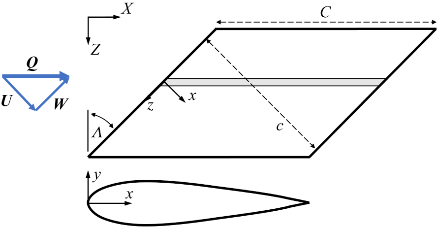
Simulations are conducted on a narrow spanwise strip of a NACA0025 aerofoil section swept at
 $45^\circ$
relative to the free stream – shown in figure 1. The NACA aerofoil section is defined in the local coordinate system aligned with the aerofoil leading edge
 $(x/c, y/c)$
. The Reynolds number is defined as
 $R_c=Qc/\nu$
, where
 $Q$
is the free-stream velocity,
 $c$
is the chord length measured normal to the leading edge and
 $\nu$
is the kinematic viscosity.
Schematic of aerofoil section used in simulations.

Figure 1. Long description
Panel A: A triangular diagram with vertices labeled U, W, and Q, and arrows indicating directions between these points. Panel B: A parallelogram with sides labeled x, z, c, and C. Arrows indicate directions along the axes labeled X, Z, and Λ. Panel C: A curved shape with axes labeled x and y, indicating a cross-sectional view of the aerofoil.
The simulations performed in this work are conducted using a massively parallel, explicit, unstructured, finite-volume, compressible flow large-eddy simulation solver for the Navier–Stokes equations developed by
 $\textrm {Cadence}^{\circledR }$
Design Systems, Inc. Details of the numerical formulation of the solver and validation cases can be found in Bres et al. (Reference Bres, Bose, Emory, Ham, Schmidt, Rigas and Colonius2018), Goc et al. (Reference Goc, Lehmkuhl, Park, Bose and Moin2021), Agrawal et al. (Reference Agrawal, Bose and Moin2024) and Fu et al. (Reference Fu, Karp, Bose, Moin and Urzay2021), among others. Fu et al. (Reference Fu, Karp, Bose, Moin and Urzay2021) in particular focused on direct numerical simulations of transitional wall-bounded turbulent flows (in the hypersonic regime) and highlighted the ‘clear trend of convergence [of WMLES] toward DNS’, building confidence in the simulation techniques used in this paper. Aspects of the formalism, including the governing equations, are highlighted here, with additional details provided in the references.
The code utilises a low dissipation spatial discretisation based on principles of discrete entropy preservation (Tadmor Reference Tadmor2003; Honein & Moin Reference Honein and Moin2004; Chandrashekar Reference Chandrashekar2013) where skew-symmetric operators are employed both to conserve kinetic energy in the inviscid zero-Mach-number limit and to conserve entropy in the inviscid adiabatic limit. These types of schemes are referred to as kinetic energy and entropy preserving. The discretisation is suitable for arbitrary unstructured, polyhedral meshes, and the solutions performed herein are computed on unstructured grids based on Voronoi diagrams. The use of Voronoi-diagram-based meshes allows for the rapid generation of high-quality grids with properties conducive to low-dissipation simulations (for instance, the vector between two adjacent Voronoi seed sites perpendicularly bisects the normal of the face that they share). Time advancement is performed using a three-stage explicit Runge–Kutta scheme (Gottlieb et al. Reference Gottlieb, Shu and Tadmor2001), and the spatial discretisation is formally second-order accurate.
The governing equations for the low-pass-filtered, compressible Navier–Stokes for mass (2.1), momentum (2.2) and total energy (2.3) are given by
 \begin{align} \frac {\partial \overline {\rho }}{\partial {t}} + \frac {\partial \overline {\rho } \tilde {u}_{\kern-1pt j}}{\partial {x_{\kern-1pt j}}} &=0 ,\\[-28pt] \nonumber \end{align}
 \begin{align} \frac {\partial \overline {\rho }\tilde {u}_i}{\partial {t}} + \frac {\partial \overline {\rho } \tilde {u}_i \tilde {u}_{\kern-1pt j}}{\partial {x_{\kern-1pt j}}} + \frac {\partial \overline {P }}{\partial {x_i}} &= \frac {\partial \tilde {\sigma }_{\textit{ij}}}{\partial {x_{\kern-1pt j}}} - \frac {\partial {\tau }^{\textit{sgs}}_{\textit{ij}}}{\partial {x_{\kern-1pt j}}}, \\[-28pt] \nonumber \end{align}
 \begin{align} \frac {\partial \overline {E}}{\partial {t}} + \frac {\partial \big[(\overline {E} + \overline {P})\tilde {u}_{\kern-1pt j} \big]}{\partial {x_{\kern-1pt j}}} &= \frac {\partial }{\partial x_{\kern-1pt j}}\left({k}\frac {\partial \overline {T}}{\partial x_{\kern-1pt j}}\right) + \frac {\partial (\tilde {u}_i \tilde {\sigma }_{\textit{ij}})}{\partial x_{\kern-1pt j}} - \frac {\partial\kern-1pt Q^{\textit{sgs}}_{j}}{\partial x_{\kern-1pt j}} - \frac {\partial \big(\tilde {u}_i \tau ^{\textit{sgs}}_{\textit{ij}} \big)}{\partial x_{\kern-1pt j}}, \\[0pt] \nonumber \end{align}
where
 $\rho$
,
 $P$
,
 $T$
and
 $u_i$
refer to the fluid density, pressure, temperature and velocity vector, respectively, and
 $i=x,y,z$
(note that the governing equations are expressed in the global Cartesian coordinate system, rather than in the sweep-aligned coordinate system defined in figure 1). The total energy, or the sum of the resolved internal and kinetic energies, is defined as
 $E = \overline {\rho }\tilde {e} + \overline {\rho }\tilde {u}_k\tilde {u}_k/2$
, with
 $k(T)$
being the thermal conductivity in (2.3). The term
 $\tilde {\sigma }_{\textit{ij}} = \mu (\tilde {T})(\tilde {S}_{\textit{ij}} - 1/3 \tilde {S}_{kk}\delta _{\textit{ij}})$
is the deviatoric part of the resolved strain-rate tensor, and
 $\tilde {S}_{\textit{ij}} = 1/2(\partial \tilde {u}_i/\partial x_{\kern-1pt j} + \partial \tilde {u}_{\kern-1pt j}/\partial x_i)$
is the resolved strain-rate tensor. The
 $(\overline {\boldsymbol{\cdot }})$
and
 $(\tilde {\boldsymbol{\cdot }})$
symbols refer to the Reynolds and Favre averaging operators, respectively. The subgrid-scale terms, indicated by the superscript ‘
 $sgs$
’, account for the stress (2.4) and heat flux (2.5) of unresolved eddies on the scales resolved by the grid and are defined respectively as
 \begin{align} \tau ^{\textit{sgs}}_{\textit{ij}} &= \overline {\rho }(\widetilde {u_i u_{\kern-1pt j}} - \tilde {u_i} \tilde {u_{\kern-1pt j}}), \\[-12pt] \nonumber \end{align}
 \begin{align} Q^{\textit{sgs}}_{j} &= \overline {\rho }(\widetilde {e u_{\kern-1pt j}} - \tilde {e} \tilde {u_{\kern-1pt j}}). \\[10pt] \nonumber \end{align}
The isotropic part of the subgrid stress is absorbed into pressure, leading to a pseudo-pressure field. The subgrid heat flux is modelled using the constant turbulent Prandtl number approximation (
 $ \textit{Pr}_t = 0.9$
) applied to the dissipative component of the subgrid stress tensor. The Mach number is low throughout this study (
 $M=0.20$
) and, at these conditions, a calorically perfect gas equation of state is adopted for air (
 $ \textit{Pr} = 0.70, \gamma = 1.4$
), while the molecular viscosity is assumed to follow a power law of temperature with an exponent of
 $0.75$
.
An equilibrium wall model is applied at the wall, but is generally inactive due to the highly refined nature of the grids in the wall-normal direction, with
 $|y^+|\lt 1$
over the entirety of the aerofoil at all combinations of Reynolds number and wall heating conditions that are considered. Note that the equilibrium wall model (Kawai & Larsson Reference Kawai and Larsson2012) is still set as the wall boundary condition despite the highly resolved nature of the mesh as a fail-safe in case
 $y^+$
ever exceeds 1 (even if only instantaneously), but the Van Driest damping function (Van Driest Reference Van Driest1956) ensures that the contribution of the wall model to the stress at the wall smoothly vanishes in the wall-resolved limit. The exact expression for the wall model used in this study can be found in Appendix A of Goc (Reference Goc2023), but is excluded here for brevity. Periodic boundary conditions are imposed in the spanwise direction,
 $z$
. In the far field, uniform inflow and non-reflecting characteristic boundary conditions are imposed on the upstream and downstream boundaries, respectively.
Regarding the subgrid-scale terms of (2.4) and (2.5), the dynamic Smagorinsky model (Germano et al. Reference Germano, Piomelli, Moin and Cabot1991; Moin et al. Reference Moin, Squires, Cabot and Lee1991) is employed. The choice of this model is suitable for the current flow regime for two reasons: (1) in wall-bounded flows, the model recovers the proper asymptotic decay of
 $\tau _{xy}^{\textit{sgs}} \sim y^3$
without the use of ad hoc corrections due to its use of the Germano identity with a dynamic test filtering procedure; and, for the same reason, (2) in laminar flows, the subgrid-scale stresses vanish. This behaviour was rigorously verified in a posteriori transitional channel flows in the original work of Germano et al. (Reference Germano, Piomelli, Moin and Cabot1991). In this paper, the influence of the subgrid-scale model on the quantities of interest is assessed via an evaluation of the activity of the model viscosity (
 $\nu _{\textit{sgs}}$
). In many turbulent flows
 $\nu _{\textit{sgs}}/\nu _{\textit{lam}}$
is often
 $\mathcal{O}(1)$
in energetic regions, with local peaks even higher. The local peaks in the transitional cases studied herein were verified a posteriori to be
 $\nu _{\textit{sgs}}/\nu _{\textit{lam}} \sim \mathcal{O}(0.01)$
, indicating a very low level of subgrid model activity. The largest peak in local viscosity ratio for any case considered herein occurred when the attachment-line boundary layer was fully turbulent at flow conditions of
 $ \textit{Re} = 3.6 {\times} 10^6, T_w / T_e = 1.4$
, where
 $\nu _{\textit{sgs}}/\nu _{\textit{lam}}$
featured a local peak value of
 $ \approx 0.15$
. Note that the viscosity ratio only serves as a surrogate for the more telling direct calculation of the dissipation ratio. Still, the peak values for subgrid-scale viscosity obtained in the present simulation are small enough to avoid modelling-error impacts, providing a low-order direct numerical simulation, as verified by comparisons with earlier simulations in all identified limiting conditions.
The grid at the aerofoil surface has a 4 : 1 aspect ratio transitioning to hexagonal close-packed polyhedral over 20 cells, using a stretching ratio of
 ${\sim }1.08$
. With the first point off the surface below
 $y^+$
= 1, this results in a wall-nominal grid with 5–6 points within
 $y^+$
= 10 for the highest-Reynolds-number case and 8–10 points for cases closer to the relaminarisation boundary. For all cases considered, there are roughly 30 points within the
 $w/W\lt 0.99$
attachment-line boundary layer. The chordwise surface distance, s, and spanwise, z, grid spacings are both fixed to four times the normal-grid spacing at the wall. The grid stretches over a height of 20 cells back to an isotropic topology. The domain width is set to
 $\Delta Z=c/32$
in the spanwise direction (corresponding to roughly
 $250 \delta _r$
) and the far field is a cylinder with radius of
 $20c$
. Results from a wider domain of
 $c/16$
show there are no confinement effects due to the
 $c/32$
domain width. The resulting grid contains roughly 140 cells in the wall-normal direction (preferentially clustered in the boundary layer),
 $2^{14} = 16\,384$
cells uniformly distributed in the chordwise direction and
 $2^{14}/32 = 512$
cells uniformly distributed in the spanwise direction, for a total of
 ${\sim }1.2\times 10^9$
cells. Limited calculations on an extremely refined grid (
 $y^+ \lt 0.5$
) showed negligible grid effects both on the relaminarisation boundary and on the temperature effects on instabilities, indicating a grid-converged solution.
3. Results
Simulations are conducted to assess the state of the boundary layer over a range of Reynolds numbers and surface-temperature ratios. The simulations can be initialised unperturbed, having only low-level numerical disturbances, or perturbed, using an instantaneous flow field from a turbulent solution at
 $\bar R =286$
,
 $T_w / T_e = 1.4$
. Results focus on the long-term asymptotic behaviour, which depends on the initial disturbances, but is not overly sensitive to the exact levels.
3.1. Laminar and turbulent profile characteristics
We first investigate the adiabatic attachment line to establish a
 $T_w / T_e \approx 1$
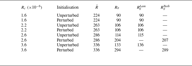
baseline and to compare to existing results in the literature. Table 1 shows the calculated
 $R_\theta$
for four different Reynolds numbers along with
 $\bar R$
calculated from the surface pressure distribution (Crouch et al. Reference Crouch, Crouch and Ng2002), and the expected laminar and turbulent
 $R_\theta$
for the given
 $\bar R$
. The results show good agreement with earlier findings for both laminar and turbulent attachment lines. Conditions leading to laminar flow, following a perturbed start, indicate relaminarisation. These
 $R_\theta$
results provide confidence in the current formulation, and indicate a relaminarisation threshold in the range
 $\bar R \approx 260{-}270$
, consistent with earlier findings discussed in § 1.
Matrix of adiabatic simulations showing comparison of
 $R_\theta$
with
 $R_{\theta }^{\textit{Lam}}$
and
 $R_{\theta }^{\textit{Turb}}$
calculated using
 $\bar R$
and the laminar and turbulent relationships given in § 1.

Table 1. Long description
A table comparing adiabatic simulation results for different Reynolds numbers and initial conditions. The table has 6 rows and 6 columns. Column headers are R subscript c (times 10 to the power of negative 6), Initialisation, R bar, R subscript theta, R subscript theta superscript Lam, and R subscript theta superscript Turb. Row 1: R subscript c, 1.6; Initialisation, Unperturbed; R bar, 224; R subscript theta, 90; R subscript theta superscript Lam, 90; R subscript theta superscript Turb, 90. Row 2: R subscript c, 1.6; Initialisation, Perturbed; R bar, 224; R subscript theta, 90; R subscript theta superscript Lam, 90; R subscript theta superscript Turb, 90. Row 3: R subscript c, 2.2; Initialisation, Unperturbed; R bar, 263; R subscript theta, 106; R subscript theta superscript Lam, 106; R subscript theta superscript Turb, 106. Row 4: R subscript c, 2.2; Initialisation, Perturbed; R bar, 263; R subscript theta, 106; R subscript theta superscript Lam, 106; R subscript theta superscript Turb, 106. Row 5: R subscript c, 2.6; Initialisation, Unperturbed; R bar, 286; R subscript theta, 114; R subscript theta superscript Lam, 115; R subscript theta superscript Turb, 207. Row 6: R subscript c, 3.6; Initialisation, Unperturbed; R bar, 336; R subscript theta, 133; R subscript theta superscript Lam, 136; R subscript theta superscript Turb, 289. Row 7: R subscript c, 3.6; Initialisation, Perturbed; R bar, 336; R subscript theta, 294; R subscript theta superscript Lam, 289; R subscript theta superscript Turb, 289.
To assess the heated wall simulations we examine the behaviour of the near-wall velocity profile. Specifically, diabatic (with heat transfer at the wall) turbulent boundary-layer velocity profiles at sufficiently high Reynolds numbers (
 $ \textit{Re}_{\tau } \gt 200$
), when appropriately non-dimensionalised, should collapse back to an adiabatic reference value. In this case, the total-stress-based velocity transformation method of Griffin et al. (Reference Griffin, Fu and Moin2021) is used, which invokes a hybrid approach where the contribution of the viscous stress to the total stress dominates in the viscous sublayer, while in the logarithmic region appeal is made to the near-balance of turbulent production and dissipation. The highest-Reynolds-number turbulent cases from the present study (
 $R_c = 3.6 {\times} 10^6$
, adiabatic) had a friction Reynolds number of
 $ \textit{Re}_{\tau } \approx 240$
, which is within the range of applicability for this transformation (
 $ \textit{Re}_{\tau } = 200 {-} 2000$
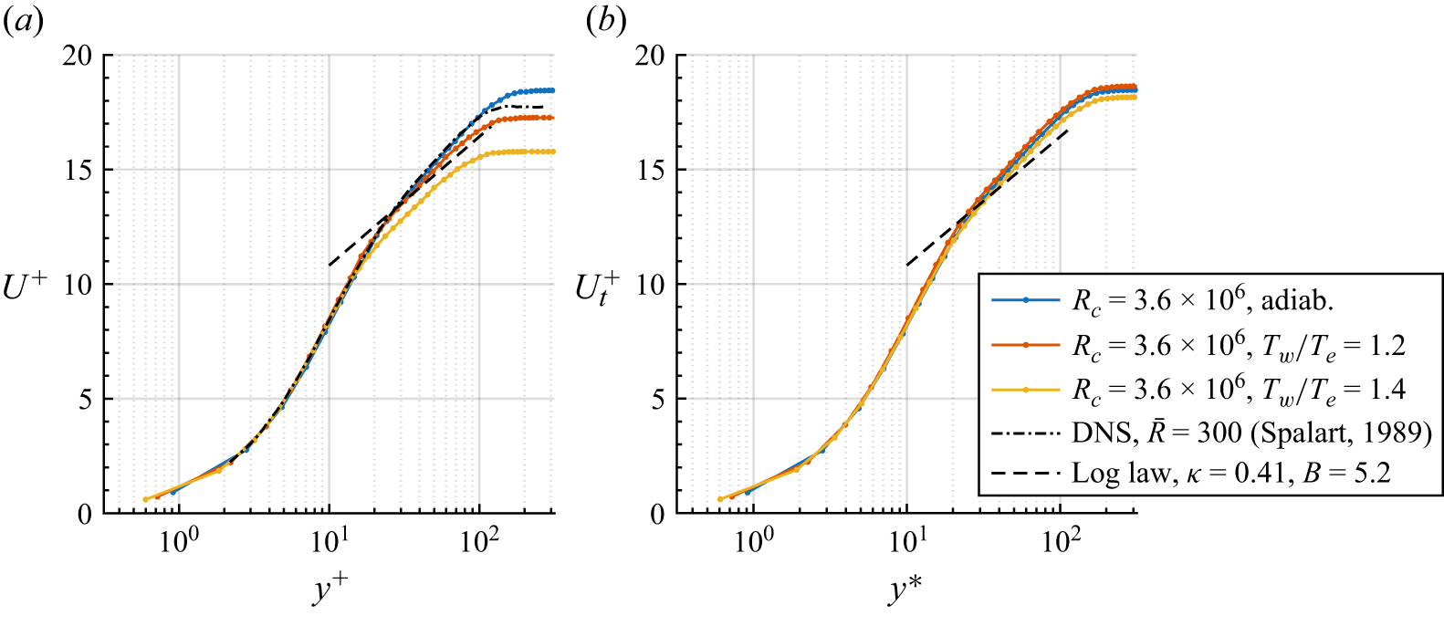
). Figure 2 shows the result of applying the total-stress-based method in Griffin et al. (Reference Griffin, Fu and Moin2021) to three velocity profiles from the present study, all at
 $R_c=3.6 {\times} 10^6$
, but with varying wall heating levels. In particular, equation (5) of that paper was used to compute the non-dimensional stress, then integrated in the wall-normal direction to find
 $U_t^+$
, or the total-stress-based viscous velocity. Results in figure 2(b) show a good collapse of the velocity profiles, on a par with reported collapses for a wide range of diabatic pipe, channel and boundary flows (Griffin et al. Reference Griffin, Fu and Moin2021). This result demonstrates that the effects of wall heating are appropriately captured (at least in the fully turbulent limit) within the current simulation campaign. In addition, figure 2(a) also includes the adiabatic result from Spalart (Reference Spalart1989) for
 $\bar R=300$
. This shows very good agreement with the current adiabatic case, with only small differences at the edge of the boundary layer due to slightly different Reynolds numbers (i.e. current value
 $\bar R=336$
).
Application of the compressible velocity transformation of Griffin et al. (Reference Griffin, Fu and Moin2021) to three high-
 $ \textit{Re}$
attachment-line profiles from the present study, with wall heating varying from adiabatic to a ratio of
 $1.2{-}1.4$
. (a) The raw profiles plotted in traditional ‘plus’ coordinates with direct numerical simulation (DNS) data at
 $\bar {R}=300$
of Spalart (Reference Spalart1989) overlaid. (b) The collapsed profiles plotted for the total-stress-based viscous velocity
 $U_t^+$
against the semi-local coordinate
 $y^*$
.

Figure 2. Long description
Two line graphs compare velocity profiles under different heating conditions. Panel A: A line graph plots the raw profiles in traditional plus coordinates. The x-axis is labeled y+ and the y-axis is labeled U+. The graph includes data series for three different heating conditions: adiabatic, Tw/Te = 1.2, and Tw/Te = 1.4, represented by blue, orange, and yellow lines respectively. Direct numerical simulation (DNS) data at Reθ = 300 from Spalart (1989) is overlaid as a dashed black line. Panel B: Another line graph plots the collapsed profiles for the total-stress-based viscous velocity against the semi-local coordinate y*. The x-axis is labeled y* and the y-axis is labeled U+_t. The same data series for the three heating conditions are represented by blue, orange, and yellow lines respectively. A log law line with κ = 0.41 and B = 5.2 is also included as a dashed black line.
3.2. Attachment-line state
As the surface temperature is increased, there are changes in the flow characteristics, which also depend on the Reynolds number. Plots of the instantaneous skin friction along the attachment line at four different flow conditions are shown in figure 3. Figure 3(a–c) corresponds to the same Reynolds number
 $\bar R=263$
, but with temperature ratio increasing from 1.2 to 1.4, and figure 3(d) shows an increase in Reynolds number to
 $\bar R=286$
at
 $T_w / T_e=1.4$
. The lines on figure 3(a) are overlaid inviscid streamlines. These images show four different flow states: laminar steady; laminar with finite-amplitude instabilities; laminar with finite-amplitude instabilities and bursting (which is intermittent in space and time); and turbulent. These qualitative assessments along with quantitative boundary-layer information (e.g.
 $R_\theta$
, as in table 1) are used to assess the flow over a range of surface temperatures.
Instantaneous skin friction magnitude contours on the attachment line (image centred at
 $y=0$
) showing the following cases: (a) laminar flow at
 $\bar R=263, T_w / T_e = 1.2$
, (b) unstable laminar flow at
 $\bar R=263, T_w / T_e = 1.3$
, (c) unstable flow with turbulent bursting at
 $\bar R=263, T_w / T_e = 1.4$
and (d) a fully turbulent flow at
 $\bar R=286, T_w / T_e = 1.4$
. Flow is into the page, and the aerofoil is swept so that the right-hand side of the image is closer to the camera than the left-hand side. The full spanwise extent of the domain is shown.

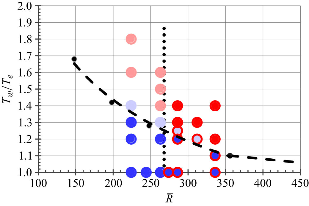
Figure 4 shows the observed boundary-layer state for a wide range of conditions simulated using both unperturbed and perturbed initialisations. The core of the symbols shows the unperturbed-start result and the outer ring shows the perturbed-start result. Thus, completely blue and completely red symbols correspond the laminar and turbulent conditions, respectively, which are not sensitive to the starting condition. Symbols with a blue core and a red ring are stable to small perturbations, but sustain turbulence when initialised as turbulent. The faded bluish and reddish symbols show laminar finite-amplitude states, without and with bursting, respectively.
Attachment-line boundary-layer state observed in simulations initialised with an unperturbed start ( ) or a perturbed start (
 ). Colour indicates the state of the boundary layer: blue (
 or
 ) = steady laminar; red (
 or
 ) = turbulent; bluish-purple (
 or
 ) = finite-amplitude instability; reddish-purple (
 or
 ) = finite-amplitude instability with bursting. Dashed lines (
 ) show a stability boundary constructed from Hall et al. (Reference Hall, Malik and Poll1984), Lasseigne et al. (Reference Lasseigne, Jackson and Hu1992) and Reed & Saric (Reference Reed and Saric2014) (
 ). Vertical dotted line (
 ) shows relaminarisation threshold.

The dashed lines in figure 4 indicate the boundary of instability constructed from earlier analyses. The curve for
 $\bar R \gt 350$
is based on the results of Hall et al. (Reference Hall, Malik and Poll1984) and Lasseigne et al. (Reference Lasseigne, Jackson and Hu1992). The curve for
 $\bar R\lt 350$
is a fit through points taken from Lasseigne et al. (Reference Lasseigne, Jackson and Hu1992) and Reed & Saric (Reference Reed and Saric2014). All unperturbed-start simulations for conditions with
 $T_w / T_e$
below the stability boundary are shown to be stable (symbols with blue core), while conditions above the stability boundary are shown unstable (symbols without blue core) – in good agreement with the earlier stability analyses.
The perturbed-start simulations indicate the propensity for sustaining turbulence. These results show an insensitivity to surface temperature, with a relaminarisation boundary that is independent of
 $T_w / T_e$
(dotted line in figure 4). For
 $\bar R$
above the relaminarisation threshold, instability is a good indicator of turbulence – below the relaminarisation threshold it is not.
3.3. Transitional flow states
An interrogation of the instability results for
 $\bar R=263$
and
 $T_w / T_e=1.3$
shows a frequency of
 $f\delta _r/W=0.0168$
and a wavelength of
 $\lambda _z/\delta _r=20.1$
. These are in reasonable agreement with unstable adiabatic results occurring at higher Reynolds numbers; for example, Joslin (Reference Joslin1996) observed a frequency of 0.0162 and wavelength of 22.9 at
 $\bar R=700$
. The heated-surface stability results of Lasseigne et al. (Reference Lasseigne, Jackson and Hu1992) show a critical wavelength of
 $\lambda _z/\delta _r \approx 20$
at
 $\bar R=356$
and
 $T_w / T_e = 1.1$
, in very good agreement with the current findings.
Below the
 $\bar R$
threshold for relaminarisation, instability leads to a finite-amplitude equilibrium state, as shown in figure 3(b). As
 $T_w / T_e$
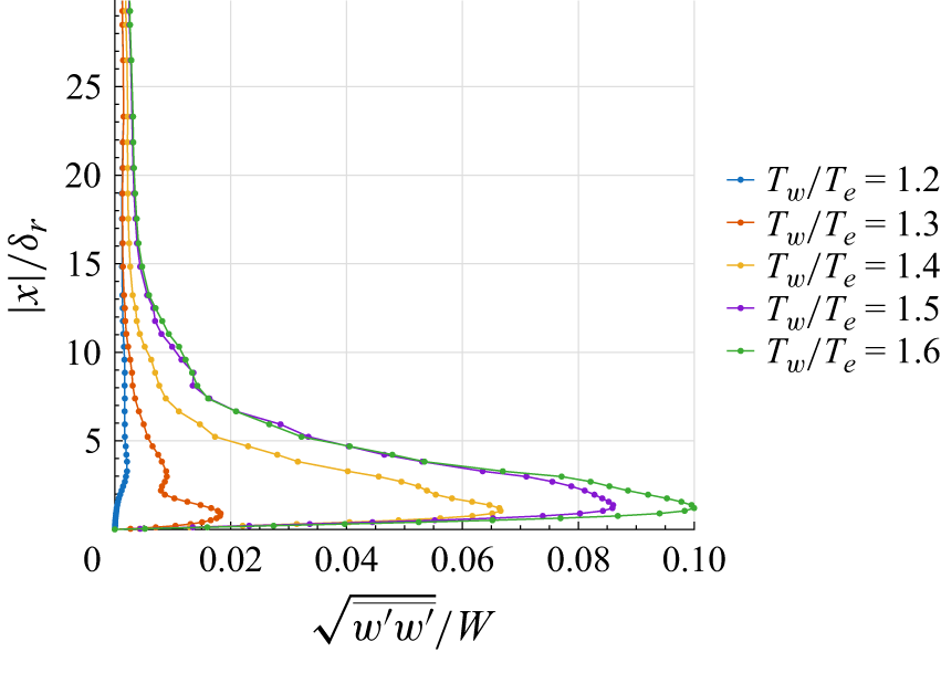
is increased above the critical value for instability, the equilibrium amplitude increases – consistent with a supercritical bifurcation. Figure 5 shows the magnitude of the fluctuating velocity profile on the attachment line corresponding to
 $T_w / T_e=1.2, 1.3, 1.4, 1.5, 1.6$
. As shown in figure 3,
 $T_w / T_e = 1.2$
is stable and
 $T_w / T_e = 1.3$
is unstable resulting in a finite-amplitude equilibrium state. For
 $T_w / T_e \geq 1.4$
, the fluctuation amplitude is significantly larger, and turbulent bursts are observed. Along with the increase in the equilibrium amplitude, the average skin friction increases 20 % between
 $T_w / T_e=1.3$
and
 $T_w / T_e=1.6$
.
Root mean square of the streamwise velocity fluctuations on the attachment line normalised by the spanwise component of the free-stream velocity, plotted against the wall-normal coordinate (
 $|x|/\delta _r$
) at
 $\bar R=263$
(
 $R_c = 2.2 {\times} 10^6$
) for varying wall-temperature ratios from
 $1.2\text{ to }1.6$
.

4. Conclusions
The simulations of this study support earlier stability analyses for attachment-line flow on a heated leading edge, which show a reduction in the critical Reynolds number as the surface-temperature ratio is increased. The results also show that the relaminarisation boundary is insensitive to surface heating. For surface-temperature ratios just above the critical value for instability, finite-amplitude equilibrium states are observed. Above the critical Reynolds number for relaminarisation, instability leads to turbulence as the surface-temperature ratio increases. Below the critical Reynolds number for relaminariation, instability leads to turbulent bursting as the surface-temperature ratio increases, but not fully turbulent flow. The bursting appears to be linked to the amplitude of the velocity fluctuations, consistent with a secondary instability, but no detailed stability assessments were conducted.
Even though the attachment line remains laminar at large surface-temperature ratios, the laminar flow is not likely to persist off the attachment line for significant distances. Earlier studies of Bertolotti (Reference Bertolotti1999) and Mack et al. (Reference Mack, Schmid and Sesterhenn2008) show that attachment-line instabilities can potentially link to downstream cross-flow instabilities. Thus, the presence of large finite-amplitude disturbances on the attachment line suggests an efficient receptivity mechanism for travelling cross-flow instabilities – with receptivity amplitudes increasing with surface-temperature ratio. Furthermore, recent results of Barahona et al. (Reference Barahona, van de Weijer, Vidales and Kotsonis2024) show that surface temperature is highly destabilising for travelling cross-flow instability. This combination of effects can be expected to lead to a fairly rapid transition off the attachment line for higher surface-temperature ratios, even for lower attachment-line Reynolds numbers.
Acknowledgements
This research used resources from the Oak Ridge Leadership Computing Facility, which is a DOE Office of Science User Facility supported under Contract DE-AC05-00OR22725 and an additional dedicated DD allocation. The authors acknowledge helpful discussions with Kevin Griffin of NREL, especially in application of the velocity transformation for variable-property flows.
Declaration of interests
The authors report no conflict of interest.
 Rθ
 RθLam
 RθTurb
 R¯
 Re
 1.2−1.4
 R¯=300
 Ut+
 y∗

 y=0
 R¯=263,Tw/Te=1.2
 R¯=263,Tw/Te=1.3
 R¯=263,Tw/Te=1.4
 R¯=286,Tw/Te=1.4
 |x|/δr
 R¯=263
 Rc=2.2×10⁶
 1.2 to 1.6


