2.1. The Malthusian state

I first introduce the model of an optimal lifecycle of individuals living in small communities and being isolated from any external cultural influence. In such an environment, natural selection favors cultural traits which maximize the rate of community growth.

Consider a model set-up in continuous time with infinite horizon. There are many isolated communities of humans, each community having its own unique cultural identity. The economy consists of a single consumption good, which, following Robson and Kaplan (Reference Robson and Kaplan2003), we interpret as energy needed to live and reproduce. Human life is divided into two stages, detailed below.

At birth, a cultural identity is formed by copying a role model, selected randomly from the same community. Since all potential role models share the same culture, the cultural transmission process is trivial as all newborn individuals simply join that culture.

In the first stage of life, humans are young and can produce two outputs: (i) the consumption good, with exogenous productivity $y$ per unit of time, and (ii) newborn children, detailed below. Young individuals also pose as role models for the newborns forming their cultural identity.

In the second stage of life, humans are old and produce neither the consumption good nor children. But they can still pose as cultural role models for the newborns.

Transition from the young to the old stage is a Poisson process with the rate of $\mu _1( c_1)$, where $c_1$ is the consumption level of young individuals. One can view $\mu _1$ as the rate of aging, that can be reduced by higher consumption.

Similarly, death of old individuals is a Poisson process with rate $\mu _2( c_2)$, where $c_2$ is the consumption of the old. Both aging rate $\mu _1({\cdot})$ and death rate $\mu _2({\cdot})$ satisfy the following conditions: $\mu _i( c)$ is continuous and finite for every $c> 0$, $\mu '_i( 0) = -\infty$, $\mu _i'({\cdot}) < 0$, and $\mu _i^{\prime \prime }({\cdot}) > 0$.

Denote the rate of population growth by $r$ and assume the measure of newborns at time $t = 0$ is normalized to unity. Then, the measure of young individuals at $t = 0$ born $x$ units of time earlier is $\exp (\! -( r + \mu ( c_1) ) x)$, and the total population of young individuals at $t = 0$ is

$$p_1( c_1,\; 0) = \int_0^\infty \exp(\! -( r + \mu_1( c_1) ) x) {dx} = {1 \over r + \mu_1( c_1) }.$$

Due to constant population growth, young population at time $t$ is $p_1( c_1,\; t) = p_1( c_1,\; 0) \exp ( rt) = {\exp ( rt) }/( {r + \mu _1( c_1) })$, and therefore the number of people becoming old at $t$ is $\mu _1( c_1) p_1( c_1,\; t) = {\exp ( rt) \mu _1( c_1) }/( {r + \mu _1( c_1) })$. The population of old individuals alive at $t = 0$ is then equal to

$$p_2( {\bf c},\; 0) = {\mu_1( c_1) \over r + \mu_1( c_1) }\int_0^\infty \exp(\! -( r + \mu_2( c_2) ) x) {dx} = {\mu_1( c_1) \over ( r + \mu_1( c_1) ) ( r + \mu_2( c_2) ) },\;$$

where ${\bf c} = \{ c_1,\; c_2\}$ is the “lifestyle” vector, i.e., the lifetime consumption profile.

A birth of a new human requires $c_0$ units of energy/consumption good. Natural selection leaves only those communities where all members have a common goal of highest population growth rate, and are pooling their resources to achieve that goal. Hence, we can perform our optimization calculations at the community level.

The total amount of energy allocated by the community to births at representative time $0$ is $( y-c_1) p_1( c_1,\; 0) -c_2p_2( {\bf c},\; 0)$ hence the mass of newly born at $t = 0$ is

(1)$$u_0( {\bf c},\; r) \equiv {( y-c_1) \over c_0( r + \mu_1( c_1) ) } - {c_2\mu_1( c_1) \over c_0( r + \mu_1( c_1) ) ( r + \mu_2( c_2) ) }.$$

By earlier assumption we have that such mass is unity, $u_0( {\bf c},\; r) -1\equiv 0$, which defines population growth $r$ as implicit function of $c_1,\; c_2$. We assume that birth requirement $c_0$ is small enough so a positive growth $r$ is feasible.

As a corollary of Proposition 1, maximization of $r$ over $c_1,\; c_2$ is equivalent to maximization of (1) over the same parameters. Because (1) is decreasing with old-age consumption $c_2$, we can conclude that the optimal such consumption is $c_2 = 0$, as old people do not contribute to new births and their consumption would create a drag on the population growth rate. This replicates the empirical conclusion of Kaplan (Reference Kaplan1994), that hunter–gatherers do not support the elderly.

Given this conclusion, (1) becomes $u_0( \{ c_1,\; 0\} ,\; r) = {( y-c_1) }/( {c_0( r + \mu _1( c_1) ) })$; its maximization yields

(2)$$-\mu'_1( c_1) {y-c_1\over r + \mu_1( c_1) } = 1$$

as the first-order condition of optimal $c_1$. Here $( {y-c_1}) /( {r + \mu _1( c_1) })$ can be interpreted as the value of remaining life of a young individual, equal to the generated food surplus $y-c_1$ times expectancy of life discounted by population growth rate, $1/( {r + \mu _1( c_1) })$. The term $-\mu '_1( c_1)$ in (2) is the marginal effect of extra consumption on the chance of remaining young; the right-hand side of (2) is the marginal cost of extra consumption.

This model fits all characteristics of a Malthusian steady state. In particular, the rise in available resources $y$ decreases mortality and increases fertility (as measured by $u_0$ for a given $r$), and therefore increases the population rate of growth.

2.2. Oblique cultural transmission

We now generalize the model of section 2.1 to add cultural transmission across communities. The mathematical concept of cultural transmission is adapted from Zakharenko (Reference Zakharenko2016a, Reference Zakharenko2016b).

Suppose that, due to rising population density and improvements in communication technology, there is probability $q$ that a newborn individual picks up a role model from outside her community. We will refer to $q$ as the cultural openness of the world's communities to each other.Footnote ³ Although previous studies assumed that potential outside role models can increase the chance of being followed by allocating effort and/or resources toward that goal, this paper assumes that the chance of a living individual, young or old, to become a role model is exogenous and does not depend on choice variables. Even this simple setting is sufficient to explain changes in human lifestyles; introducing special effort to become a role model would only reinforce the conclusions of this paper.

To account for the empirical fact that some individuals have many more followers than others, in the discussion of testable predictions we will assume that the idiosyncratic ability to become a role model is heterogenous. At the same time, the distribution of such ability is the same across all communities, hence the rate of attraction of outside new individuals into a community is merely proportional to its population size. Thus, the distribution of ability to become a role model is immaterial for the rate of community growth and therefore does not affect optimal lifestyles.

Since we account individuals by their culture, not their genotype, new individuals who picked external cultural types migrate to the community of their role models. Each community therefore retains only fraction $1-q$ of those born in that community, but it also recruits new individuals via oblique cultural transmission from outside. Denote by followers of a given community newborn individuals who are joining that community, regardless of their community of birth. Assuming each community has a negligible share in the global population, the number of followers at time $t$ attracted from outside is $( {q}/{P}) ( p_{1}( c_1,\; t) + p_{2}( {\bf c},\; t) )$, where $P$ is the ratio of global population to global number of births, so that $1/P$ is the global birth rate.

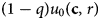
Suppose the number of community followers at a representative time $0$ is normalized to unity. The number of births by parents of that cultural type is still given by (1), hence the number of followers recruited via vertical cultural transmission (i.e., those born in the same community) is $( 1-q) u_0( {\bf c},\; r)$.

Denote

(3)$$p( {\bf c}) \equiv p_1( c_1,\; 0) + p_2( {\bf c},\; 0) = {1 \over r + \mu_1( c_1) } \left(1 + {\mu_1( c_1) \over r + \mu_2( c_2) } \right)$$

the ratio of community population to the number of followers. The total number of followers of the community in question, recruited via both vertical and oblique cultural transmission, is given by

(4)$$\eqalign{u_1( {\bf c},\; r) & \equiv ( 1-q) u_0( {\bf c},\; r) + {q\over P}p( {\bf c}) \cr & = {1 \over r + \mu_1( c_1) } \left({( 1-q) ( y-c_1) \over c_0} + \frac{q}P + \left(\frac{q}P-{( 1-q) c_2\over c_0} \right){\mu_1( c_1) \over ( r + \mu_2( c_2) ) }\right)}$$

By earlier assumption, $u_1( {\bf c},\; r) -1\equiv 0$, which defines the rate of community growth $r$ as implicit function of lifestyle ${\bf c}$. Proposition 1 applies to $u_1({\cdot})$, too, hence maximization of $r$ is equivalent to maximization of (4) over ${\bf c}$. Maximization over old-age consumption $c_2$ yields the following first-order condition:

(5)$$-\mu'_2( c_2) V_2 = 1,\; $$

where $V_2\equiv \left[Q-c_2\right]\ ( 1/( {r + \mu _2( c_2) })$ and where $Q\equiv {qc_0}/( {P( 1-q) })$. Here $Q$ is cultural productivity, i.e., the number of followers that can be attracted from outside by a role model, relative to the number of followers born within the community, per unit of consumption good spent on births. The value of $Q$ is exogenous for a given community. $V_2$ can be interpreted as the value of remaining life of an old individual; in its definition, the term in square brackets is the contribution of such individual to community population growth via attraction of followers from outside, whereas the term $1/( {r + \mu _2( c_2) })$ is the expectancy of remaining life, discounted by population growth rate. The interpretation of (5) is similar to that of (2), that the marginal effect of consumption on mortality, times the value of remaining life of the old, equals the marginal cost of consumption. Note that $c_2$ defined by (5) maximizes not only the overall objective (4), but also $V_2$.

Maximization of (4) over young-age consumption $c_1$ yields

(6)$$-\mu'_1( c_1) ( V_1-V_2) = 1,\; $$

where $V_1\equiv ( {y + Q-c_1 + \mu _1( c_1) V_2}) /( {r + \mu _1( c_1) }$. The latter is the value of remaining life of a young individual, where $y + Q-c_1$ is the contribution to community population growth, via consumption good donation and via posing as role model; $\mu _1( c_1) V_2$ is the rate of transition into the old age times the value of such age. Optimal young-age consumption $c_1$ given by (6) maximizes not only the overall objective, but also the value of $V_1$.

2.3. Cultural openness: community effects

Suppose all communities have initially optimal (and therefore identical) lifestyles. Suppose further that cultural openness $q$ increases. What is the optimal lifestyle of a “pioneer” community in the changed world, assuming that the lifestyles of other communities, and therefore the global birth rate, remain at the initial level?

First, observe from (4) that in the initial symmetric equilibrium, we have that $p = P$, hence equality $u_1\equiv 1$ requires $u_0 = 1$, hence a marginal change in $q$ has no direct effect on $u_1$, hence it also does not directly affect the community growth rate $r$. Intuitively, in the symmetric equilibrium the number of newborns emigrating to other communities equals the number of newborns immigrating from other communities; a greater cultural openness increases both numbers without changing the total. Therefore, a marginal increase in $q$ only affects the changing lifestyle ${\bf c}$.

We can now state the key results of the model.

In words, rising return to “telling tales,”  i.e., to posing as a role model for external followers, makes individuals increase investment into survival as their capability to “tell tales” is less age-sensitive (in this stylized model, completely independent from age) than their capability to generate food surplus. Such increasing interest in own survival makes individuals appear more focused on own consumption, consistently with the observed pattern of demographic transition. Also, the theorem predicts that the old age consumption $c_2$ rises with cultural openness $q$ despite zero amount of consumption good being produced, meaning that old-age support is increasing.

Proof. We have that

$${{d}{V_2}\over {d}{q}} = {\partial{V_2}\over \partial{q}} + {\partial{V_2}\over \partial{r}}{\partial r\over \partial q} + {\partial{V_2}\over \partial{c_2}}{\partial c_2\over \partial q}.$$

But the effect via $r$ is zero because ${\partial r}/{\partial q} = 0$, whereas the effect via $c_2$ is zero due to the envelope theorem, as ${\partial V_2}/{\partial c_2} = 0$. Therefore, the total effect equals partial effect ${\partial {V_2}}/{\partial {q}}$, which is positive: greater cultural openness allows role models to attract more followers from outside, which makes the life of a role model more valuable. Then, from (5) and properties of $\mu _2({\cdot})$, higher value of life $V_2$ must result in higher investment $c_2$ to preserve this life.

The same logic applies to show that ${{d}{V_1}}/{{d}{q}} = {\partial V_1}/{\partial q}$. Next, observe that

$$\eqalign{V_1-V_2 & = {y + Q-c_1\over r + \mu_1( c_1) } - {r\over r + \mu_1( c_1) }V_2 \cr & = {y-c_1\over r + \mu_1( c_1) } + {Q\mu_2( c_2)\over ( r + \mu_1( c_1)) ( r + \mu_2( c_2) )} + {c_2r\over ( r + \mu_1( c_1) ) ( r + \mu_2( c_2) ) },\; }$$

which increases with $\it Q$ which in turn increases with $\it q$. Hence, ${\partial ( V_1-V_2) }/{\partial q}> 0$, that is, the value of young life $V_1$ not only increases, but does so faster than $V_2$, with $q$. But then, according to (6), consumption of the young $c_1$ increases, as well.  □

What is the effect of increasing cultural openness on fertility and birth rates? Define the former as the ratio of newborn to fertile (i.e., young) population, whereas the latter as the ratio of newborn to all community population. Then, fertility rate is formally given by $1/{p_1( c_1,\; 0) } = r + \mu _1( c_1)$, which decreases as higher $q$ causes $c_1$ to rise and $\mu _1$ to fall. The birth rate is $1/{p( {\bf c}) }$; the theorem below studies its change.

Proof. Theorem 1 has shown that rising $q$ causes consumption at all stages of life to increase. From the definition (3) of $p( {\bf c})$, it is unambiguously increased by rising $c_2$. The effect of rising $\it c_1$

$$\quad {\partial p\over \partial c_1} = {-\mu'_1( c_1) \over ( r + \mu_1( c_1) ) ^2}{\mu_2( c_2) \over r + \mu_2( c_2) }$$

is positive, too, hence higher cultural openness causes $p( {\bf c})$ to increase, as well. It also causes the birth rate $1/p$ to decrease.

The problem of maximization of (4) over ${\bf c}$ is the problem of tradeoff between producing new births $u_0$ and posing as role models $p$, where the price of the latter in the currency of the former is given by ${q}/{( 1-q) P}$. As this price increases, the previous paragraph shows that $p$ must increase; but then, $u_0$ must decrease: increasing $p$ without decreasing $u_0$ would mean that the value of (4) under the initial value of $q$ could have been improved too and therefore was not optimal.  □

As $p$ rises from initial value of $P$ while $u_0$ declines from initial value of unity, the term ${p}/{P}$ in (4) becomes greater than $u_0$, meaning that ${\partial u_1}/{\partial q}> 0$. The latter result also means ${{\rm d}{r}}/{{\rm d}{q}}> 0$; the proof is similar to that of Proposition 1. In words, an increase in cultural openness $q$ will eventually cause communities that adapt sooner to grow faster than the rest of the world, despite lower birth rates. Growth occurs because pioneer communities, by having greater longevity, pose as more influential role models and attract many cultural followers from outside. As the adapted communities grow faster than others, their lifestyle eventually spreads while old lifestyles become extinct.

2.4. Cultural openness: aggregate effects

We now analyze how the global population growth is affected by rising cultural openness. As explained at the beginning of section 2.3, when all communities behave equally optimally, the number of births per community $u_0( {\bf c},\; r)$ must be equal to the number of new followers $u_1( {\bf c},\; r)$, which was in turn normalized to unity. Therefore, the global population growth rate $r$ is implicitly defined by identity $u_0( {\bf c},\; r) \equiv 1$ and does not directly depend on cultural openness $q$, only via lifestyle ${\bf c}$.

Theorem 2 has shown that greater cultural openness $q$ causes function $u_0$ to decrease, for given $r$, via rising consumption ${\bf c}$. But then, according to Proposition 1, the global rate of population growth $r$ also decreases with cultural openness, via the same channel. This result explains demographic transition by changing pattern of cultural transmission.

2.5. Notable individuals

This section discusses testable predictions of the model. There are no direct measures of who was influenced by whom; at the same time, there are data on individuals who have arguably influenced many people: individuals with biographical Wikipedia pages translated into multiple languages. We will assume that such pages are created and used by followers who were attracted via oblique cultural transmission, as those attracted by vertical transmission (i.e., biological relatives) are relatively small in numbers and usually use other ways to commemorate their ancestors.

Suppose there are thresholds $z_1,\, \ldots ,\; z_n, \ldots$ such that an individual's biography is translated into $n$ languages on Wikipedia if her number of followers was within $[ z_n,\; z_{n + 1})$. Because the idiosyncratic number of followers can be highly stochastic for any given lifestyle, assume individuals differ in their cultural attractiveness $a\geq 0$, such that the individual number of followers attracted per unit of time from other communities is proportional to $a$. Assume also that individual $a$ is determined at birth and remains the same throughout life, but does not affect the lifestyle ${\bf c}$. The distribution of $a$ is assumed to be the same across communities and birth cohorts, and is such that mean $a$ is unity.

Then, an individual who has lived $t$ years and had cultural attractiveness $a$ must have attracted ${aqt}/P$ followers in expectation. This number depends not only on aggregate parameters $q,\; P$ and idiosyncratic shock $a$, but also on duration of life $t$ which is in turn affected by chosen lifestyle ${\bf c}$. Section 2.3 shows that communities that adapt to rising cultural openness sooner than others should have lower fertility/birth rates and greater life expectancy; they also should attract more followers from other communities. This gives rise to the following two testable hypotheses, relating fame (as measured by the amount of Wikipedia information) and demographic variables.

Furthermore, section 2.3 predicts that, because individuals with many followers tend to have lower fertility and mortality, their presence should eventually reduce fertility and mortality of other people around them. As we do not know where exactly the followers of each notable individual lived, I make an identifying assumption that, in the pre-television era (i.e., before 1950), cultural influence occurred primarily within the national borders. Then, we can formulate two more testable predictions about the effect of notable individuals (i.e., those with a biographical Wikipedia page in at least one language) on the general public:

The next section develops empirical strategies to verify each of the above hypotheses.

3.1. Fertility of notable individuals

This section tests Hypothesis 1. First, I directly compare fertility of notable females (treatment group) to that of the general population (control group). The focus on females is due to more accurate measures of their fertility; most general population surveys do not even ask males about their number of children.

The data on control group fertility are from U.S. National Health Interview Survey [NHIS, Blewett et al. (Reference Blewett, Drew, Griffin, King and Williams2018)], a representative repeated cross-section of U.S. population. I use data from years 2000, 2005, 2010, and 2015, when female respondents were asked about their number of live children ever born. Control group is defined as females who have reached age 45 (i.e., most likely have completed their fertility) by the time of the interview. Control variables that were used include age, education, occupation, income group, and the number of hours worked per week.

The data on treatment group fertility were based on Pantheon 1.0 dataset [Yu et al. (Reference Yu, Ronen, Hu, Lu and Hidalgo2016)]. These data include all individuals whose biographical Wikipedia pages were translated into at least 25 languages as of May 2013, totaling 11,341 individuals. For each individual, the data provides the year and location of birth, gender, occupation, as well as some measures of their popularity on Wikipedia. We also collected some additional information, via both automated queries from Wikidata (a database that standardizes Wikipedia information) and manually. In particular, country of citizenship information of each notable individual was collected from Wikidata. This allows us to identify the treatment group as all Pantheon females born between 1880 and 1970, alive in 2000, who lived 45+ years, with United States listed as their country of citizenship, totaling 267 individuals.

The educational level of each member of the treatment group was first queried from Wikidata (property “academic degree”, P512), with an attempt to map each result to the standardized educational classification used by NHIS. The latter classification has 22 categories ranging from “kindergarten only” to “Doctoral degree.” Finally, a manual biographical search was conducted verify or update all information.

Although Wikidata has the “number of children” entry (P1971), the information is often missing or incorrect. For this reason, we studied the biography of each member of the treatment group and recorded the most credible information on the number of live births.Footnote ⁴ Both education and fertility were recorded in September 2018, when all members of treatment group were 48+ years old.

Table 1 compares the distribution of fertility in control and treatment groups. A sharply lower fertility of notable women is clearly visible. Among the top four women by Wikipedia pageviews (Jennifer Aniston, Whitney Houston, Mariah Carey, and Sandra Bullock), the total number of children is three, two of which are twins.

Table 1.

Distribution of fertility: general population (control) vs. celebrities (treatment)

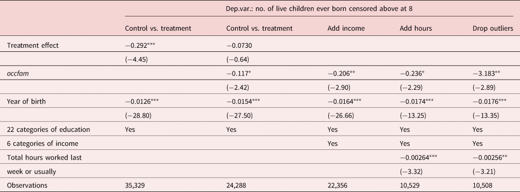
To control for the birth cohort and detailed education, I pool control and treatment samples and run an ordered probit regression with nine categories ($0,\; 1,\; \vskip 2pt\cdots \vskip-2pt,\; 7,\; 8$+) for the number of children as dependent variable, predicted by “treatment effect” (i.e., dummy equal to one for Pantheon observations, zero for NHIS observations), year of birth and detailed educational dummies as explanatory variables. The results are shown in column 1 of Table 2; notable females have significantly lower fertility even after controlling for education and birth cohort.

Table 2.

Notable individuals and fertility, U.S. women aged 45+

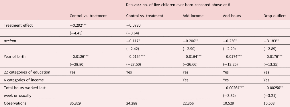
Ordered probit regression results. occfam is occupational fame (notable individuals per 1,000 employees).

t statistics in parentheses.

$^{\ast }$${\rm p}< 0.05$, $^{\ast \ast }$${\rm p}< 0.01$, $^{\ast \ast \ast }$${\rm p}< 0.001$.

This regression does not account for career choices and outcomes of women which may drive the results. For example, women who spend many hours at work may become more notable and have fewer children at the same time. Although work effort can be explained by preference/lifestyle heterogeneity detailed in section 2.3, it can also depend on economic constraints such as unobserved ability. Furthermore, in many cases women become notable after age 45, when all fertility decisions must have already been made, which creates a causality problem with above approach.

To address these problems, I try another approach. Using the data on occupations of notable females, I create a measure of occupational fame, defined as the chance of becoming notable for every given occupation. Then, I use this measure as proxy for a person's effort to become a role model, and study whether occupational fame is related to fertility outcomes within the NHIS sample. To isolate occupational fame from other effects of occupation, I control for income level and the number of hours worked.

Within the time span of NHIS data used in this paper, there were several occupational classifications used; the universe of respondents reporting their occupation has been changing, as well. In this section, I use occupational classification used in 2004–2015, hence year 2000 was dropped in the rest of the section. I match this classification to the one used in the Pantheon dataset. Then, “fame” of each occupation $j$ in 2004–2015 classification was defined as

$$occfam_j = {\sum_{t = 2004}^{2015} n^{Pantheon}_{\,jt}\over \sum_{t = 2004}^{2015} n^{NHIS}_{\,jt}},\;$$

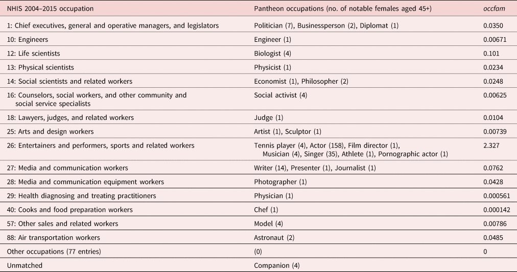
where $n^{Pantheon}_{jt}$ is the number of women in the Pantheon dataset with occupation $j$, U.S. citizenship, alive and aged 45+ in year $t$, whereas $n^{NHIS}_{jt}$ is the total number of U.S. women with the same characteristics, as estimated from the NHIS database. Occupational fame was calculated only for NHIS women who reported being employed; observations of unemployed women (who have higher fertility and who would reinforce our results) were dropped. Table 8 illustrates the matching and the calculated occupational fame.

The second regression in Table 2 repeats the first regression, dropping year 2000, dropping unemployed NHIS respondents, and adding the occupational fame as regressor for both treatment (Pantheon) and control (NHIS) groups. As expected, higher fame potential of the chosen occupation is related to lower fertility, which we interpret as evidence that cultures driving individuals to seek fame also drive them to have fewer children. At the same time, controlling for occupational fame, the treatment effect becomes insignificant (i.e., Pantheon population does not significantly differ from the NHIS sample), which can be explained by the idea that, for a given occupation, the actual fame is highly stochastic and often arrives after fertility choices have been made, regardless of what these choices were.

The observation that occupational fame potential is a better covariate of fertility than actual fame allows us to drop Pantheon individuals, whose income and work effort are unknown, and to add these control variables in a regression with NHIS respondents only. The third and fourth regressions in Table 2 report the results; the effect of occupational fame remains negative and significant after controlling for work effort and income.

Table 8 in Appendix A demonstrates that the vast majority of notable females are actors, which makes the corresponding NHIS occupation a strong outlier in its occupational fame. To make sure that the effect of such fame on fertility is not merely an actor fixed effect, the last regression in Table 2 drops observations with NHIS occupational code 26 that includes actors. The effect of occupational fame on fertility increases tenfold, which implies a convex relationship between the two.

To summarize, we find evidence that the choice of occupations associated with greater fame potential is also associated with significantly lower fertility of females; this effect cannot be explained by differences in education, income, and the number of hours worked. This result is in line with the theory of section 2.3, that there is a tradeoff between biological fitness (number of children) and cultural fitness (number of followers of one's culture).

3.2. Mortality of notable individuals

This section tests Hypothesis 2. Montagu (Reference Montagu1994) studies life expectancy of famous men from antiquity, as listed by the Oxford Classical Dictionary. Dropping those who died from violent deaths, average lifespan of remaining celebrities is 72 years, which is equal with high degree of statistical confidence to that of their counterparts from the same dictionary who died between 1900 and 1950. de la Croix and Licandro (Reference de la Croix and Licandro2015) study a rich dataset of 300,000 notable individuals from the entire human history and conclude that their life expectancy has always been significantly higher than that of the general population and, moreover, started to increase at least a century before that of the general population. These observations confirm the idea that fame has always selected long-lived individuals, and that celebrities pioneered demographic change.

3.2.1. Modern comparisons

The NHIS dataset described above has followed up the survival status of its respondents, which allows one to use these data for mortality studies. This section conducts an analysis similar to that of section 3.1 to investigate mortality difference between modern Pantheon individuals and NHIS respondents.

For the purposes of this section, the control group was defined as all individuals, males and females, observed in NHIS between years 1986 and 1995, aged 45 or older at the time of observation. During this period, classifications of education, income, and occupation were different from those of section 3.1, which required respective control variables to be redefined. In 2015, NHIS followed the survival status of control group members; in case of death prior to 2015, the year of death was recorded.

The treatment (i.e., notable) group was defined as all individuals, males and females, from the Pantheon dataset, born in 1950 or earlier, alive in 1986, who lived 45+ years, with United States listed as their country of citizenship, totaling 976 individuals.

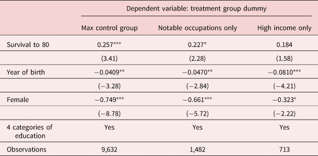
First, I investigate whether survival from age 60 to 80 increases the chance of becoming famous (i.e., of being a member of the treatment group). I pool 9,408 members of the control group aged 60 at the time of observation with 224 members of the treatment group born in years 1926–1935 (i.e., who also turned 60 in 1986–1995). I then run a probit regression with treatment group dummy as the dependent variable and dummy for survival to age 80 as the main explanatory variable. The controls include year of birth, gender, and education.

The results are presented in the first column of Table 3. The second column narrows the control group only to individuals with positive occupational fame, i.e., with occupations observed among the treatment group members. In both regressions, survival plays a positive and significant role in becoming famous. The last column further narrows the control group to individuals with family income of $50,000 and above (the highest category), as members of the treatment group are likely to belong to upper income strata. The effect of survival is positive but insignificant. The latter result may be due to incorrect specification of the control group (since some Pantheon individuals may have family income below $50,000), or due to the fact that fame is associated with income rather than with longevity. Thus, the lack of data about income of Pantheon individuals prevents making a definitive comparison of the two groups.

Table 3.

Effect of survival from 60 to 80 on celebrity status

Probit regression results. t statistics in parentheses.

$^{\ast }$${\rm p}< 0.05$, $^{\ast \ast }$${\rm p}< 0.01$, $^{\ast \ast \ast }$${\rm p}< 0.001$.

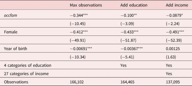
Like in section 3.1, I use an alternative approach of replacing actual fame status by a measure of occupational fame. For every occupation in the 1986–1995 NHIS classification, a measure of occupational fame was constructed, similar to that of section 3.1, separately for males and for females. Like in the 2004–2015 classification (cf. Table 8), the highest fame is expected in show business, namely among “writers, artists, entertainers, and athletes”: the chance of becoming famous is estimated at 1.04 per 1,000 employees for males and 0.357 for females. Because occupation is typically chosen earlier in life, I reverse the chain of causality and investigate the effect of occupational fame on survival of individuals aged 45 and above. Focusing on members of the control group only (i.e., on NHIS data) allows to include detailed income information into the regression.

The econometric method used is the Cox proportional hazards model. Individuals enter the model at age 45 or in year 1986, whichever occurred later. They exit the model at death or in year 2015, whichever occurred earlier. Table 4 reports estimated factors of mortality; the effect of occupational fame is negative and significant. This finding can be interpreted as evidence that cultures driving individuals to seek fame also drive them to invest more into longevity.

Table 4.

Factors of mortality

Cox proportional hazards model. occfam is occupational fame (notable individuals per 1,000 employees). t statistics in parentheses.

$^{\ast }$${\rm p}< 0.05$, $^{\ast \ast }$${\rm p}< 0.01$, $^{\ast \ast \ast }$${\rm p}< 0.001$.

3.2.2. Historical comparisons

The previous section studies modern United States, i.e., a society which experienced demographic transition for a long time, and in which lifestyles of the general population could have already converged to those of celebrities. A potentially more interesting setting is a pre-transition society, where most people still followed the Malthusian/Darwinian culture of maximizing population growth.

Historical general-population surveys are ill-suited for the purpose, as they do not track survival of individuals over time. For this reason, I study correlation between longevity and fame on a group of individuals who share the same occupation: high-ranked catholic priests. Specifically, I study all representatives, recorded in Wikidata, of three ranks below the Pope: cardinals (Wikidata item Q45722), archbishops (Q48629921), and bishops (Q611644). This choice is driven by two considerations. First, catholic priests are probably the best-recorded profession in the world, with Wikidata records spanning from birth year 1 A.D. (Apostle Peter) until modern times. In the vast majority of cases, the year of appointment, location of service, and the year of death are known; the year of birth is known in 78% of cases. Second, because catholic church is a centrally managed hierarchical institution, priests of the same rank are likely to have similar backgrounds and living standards, which makes heterogeneity in unobserved control variables much smaller than that of, say, painters or mercenaries.

A total of 32,565 individuals of the above three ranks were observed; of them, we focus on 20,105 who were born in the 19th century or earlier (so their lifespan is completed) and for whom a meaningful longevity (0 to 120) could be inferred from birth and death years. The level of fame of priests is measured by the number of language versions of their Wikipedia biographical pages, denoted numlang henceforth, ranging from zero (when an individual was cataloged in Wikidata, but no biographical text was created) to 193 (Augustine of Hippo). The popes were not studied separately due to very low variation in the number of biographical pages, with 95% of popes having numlang between 60 and 90.

The mean (standard deviation) number of languages is 3.10 (7.15). Not surprisingly, it varies with priest rank: 11.86 (13.30) among 1,931 observed cardinals, 3.26 (6.31) among 3,780 individuals with highest observed rank of archbishop, and 1.89 (5.04) among remaining 14,394 individuals with highest observed rank of bishop.

To control for time trends, a century variable was created, equal to the century of birth.

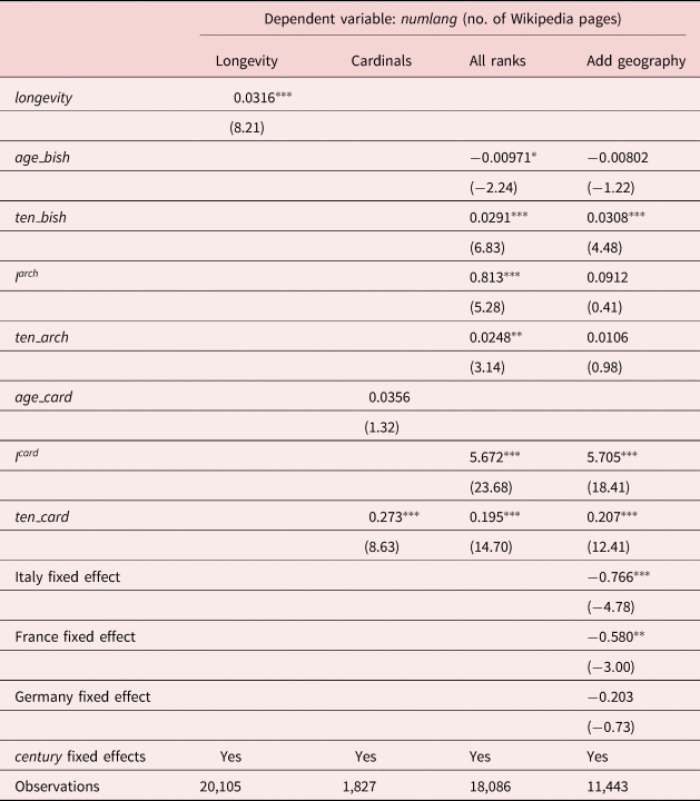
The regression results are presented in Table 5. The first column shows that longevity, i.e., age at death, is indeed positively associated with fame, controlling for century fixed effects: a Wikipedia biography in one extra language is associated with about 30 extra years of longevity.

Table 5.

Effects of longevity and tenure of Catholic priests on fame

t statistics in parentheses.

$^{\ast }$${\rm p}< 0.05$, $^{\ast \ast }$${\rm p}< 0.01$, $^{\ast \ast \ast }$${\rm p}< 0.001$.

To illustrate the effect of longevity for a given priest rank, the second regression in Table 5 focuses on cardinals only. The regression equation is

$$numlang_i = \alpha_0 + \alpha_{card} age\_card_i + \gamma_{card} ten\_card_i + \sum_t \delta_tI( century_i = t) + \epsilon_i,\;$$

where $age\_card_i$ is age at the moment of appointment as cardinal, whereas $ten\_card_i$ is tenure as cardinal, i.e., time span from appointment until death. The regression shows that tenure as cardinal indeed strongly affects fame, with biography translated into an extra language after every $1/{0.273} = 3.7$ years of tenure. The age at appointment, on the contrary, is insignificant for fame, which indicates that tenure as cardinal affects fame via its terminal margin (i.e., living longer) rather than opening margin (i.e., becoming a cardinal at younger age).

The third regression investigates the effect of tenure in each rank on fame. The regression equation is

(7)$$\eqalign{ numlang_i & = \alpha_0 + \alpha_{bish} age\_bish_i + \gamma_{ten\_bish} ten\_bish_i + \beta_{arch} I^{arch}_i + \gamma_{arch} ten\_arch_i \cr & \hskip1pc + \beta_{card} I^{card}_i + \gamma_{card} ten\_card'_i + \sum_t \delta_tI(century_i=t) + \epsilon_i.} $$

Here $ten\_card'_i$ is the same as $ten\_card_i$, with missing values (if the person has never been a cardinal, or if the date of appointment is unknown) replaced by zeros. $ten\_arch_i$ is tenure in the rank of archbishop or higher, i.e., number of years since appointed archbishop until death. In some observations, the rank of archbishop was not recorded but implied by a higher recorded rank of cardinal; in this case I assumed $ten\_arch_i = ten\_card'_i$. In all remaining cases (person never became an archbishop, or date of appointment was not recorded and could not be imputed), I assumed $ten\_arch_i = 0$.

Similarly, $ten\_bish_i$ is tenure in the rank of bishop and higher, i.e., number of years since appointed bishop until death. If the rank of bishop was not recorded but implied by higher recorded rank, I assumed $ten\_bish_i = ten\_arch_i$. If $ten\_bish_i$ was still unknown, the observation was dropped.

To control for the possibility that a mere fact of higher-rank appointment, regardless of tenure, makes the individual more famous, I add a fixed effect for archbishop rank $I^{arch}_i$ (as observed or imputed by higher rank of cardinal) and for cardinal rank $I^{card}_i$. Finally, age at appointment as bishop was defined as $age\_bish_i = longevity_i - ten\_bish_i$.

Note that tenure effects are cumulative, e.g., one extra year as cardinal increases fame by $\gamma _{bish} + \gamma _{arch} + \gamma _{card}$. Therefore, $\gamma _{arch}$ should be viewed as the additional effect of archbishop status, relative to that of bishop, whereas $\gamma _{card}$ is the additional effect of cardinal status, relative to that of archbishop.

The fourth regression repeats the third regression (cf. (7)), with added geographical controls, namely dummies for priests associated with modern Italy (3,822 out of 11,443 observations), France (1797), and Germany (741). The associated country was determined from the following information, ranked from highest to lowest priority: location of death of a cardinal, diocese of an archbishop, location of death of archbishop or bishop, location of birth.

The results of the third and fourth regressions indicate that tenure has a positive and robust effect on fame of a priest, although the difference between bishops and archbishops is not always significant. There is no robust effect of age at appointment as bishop, meaning, again, that tenure affects fame primarily via its terminal margin—longer life.

This finding confirms Hypothesis 2, that people who live longer tend to become better known and may have a stronger effect on preferences of future generations. Although the church has always encouraged high fertility, its very existence could have contributed to the emergence of preference for long life, as its most notable representatives were long-lived. The emergence of preference for longevity, in turn, has eventually led to demographic transition.

3.3. Notable individuals are influential

Hypotheses 3 and 4 predict that a larger initial number of notable individuals per capita should lead to a faster spread of their values to the general population, thus should be associated with lower birth and death rates, respectively, at some later point in time. This section tests these hypotheses empirically. Because it is not known exactly who was influenced by which role model,Footnote ⁵ our analysis is based on very loose assumptions about such influence and is therefore subject to large measurement error in the main explanatory variable.

I assume that influence has certain geographic and time limits; then, within these limits I create measures of per-capita density of notable individuals, and study whether the variation in this influence measure can explain variation in birth and death rates.

The geography of influence is assumed to be limited to national borders. This assumption is justified by the idea that country borders often separate different ethnicities whose cultural contact with each other is restricted by linguistic barriers. Geographic limits of influence were especially tight before the advent of television which dramatically reduced the cost of cultural influence; we therefore focus on data before 1950, when television arrived.

For the purposes of this section, a notable individual is defined as any individual with a Wikipedia page in at least one language; information about a total of 624,657 individuals, born between 1600 and 1920, with known year and location of death, was downloaded.Footnote ⁶ Information about location of birth and citizenship, if available, was downloaded too. Every individual was associated with a modern country, using the following information in order of decreasing priority: country of citizenship, location of death, location of birth.

Every notable individual is assumed to be influential in her country from age 30 until the moment of death. Due to such loose assumption about the timing of influence, we cannot identify the effects of influence from within-country time variation alone, and therefore cannot use country fixed effects in the regressions. Random-effects models were used instead.

For a per capita measure of influence, population data was primarily taken from the Maddison dataset [Bolt et al. (Reference Bolt, Inklaar, de Jong and van Zanden2018)], complemented by census data from Iceland, Luxembourg, and Russia.

Two per-capita measures of influence were constructed, separately for each gender. Variable pcF is the number of living notable females aged 30+ per thousand of population; the measure for males is analogous. Both variables are for 111 modern countries of the world, coinciding with those from the Barro–Lee dataset introduced below, with the time span from 1750 until 1950. In 1750, 28 of 111 countries had a positive measure of female influence pcF; by 1950, this number had increased to 96.

In our regressions, we control for aggregate levels of education and income. The education is measured by total years of schooling, population aged 15–64, as provided by Barro and Lee (Reference Barro and Lee2013). This is a balanced panel of 111 countries, with gender-specific observations every 5 years from 1870 to 2010. Educational levels inside the 5-year intervals were linearly interpolated. For birth rate studies, I use educational level of women only (variable tyrF), as it is regarded as stronger predictor of fertility. In death rate studies, education of both genders were used. Income is GDP per capita as measured by the Maddison dataset [Bolt et al. (Reference Bolt, Inklaar, de Jong and van Zanden2018)], denoted as gdp.

3.3.1. Birth rate

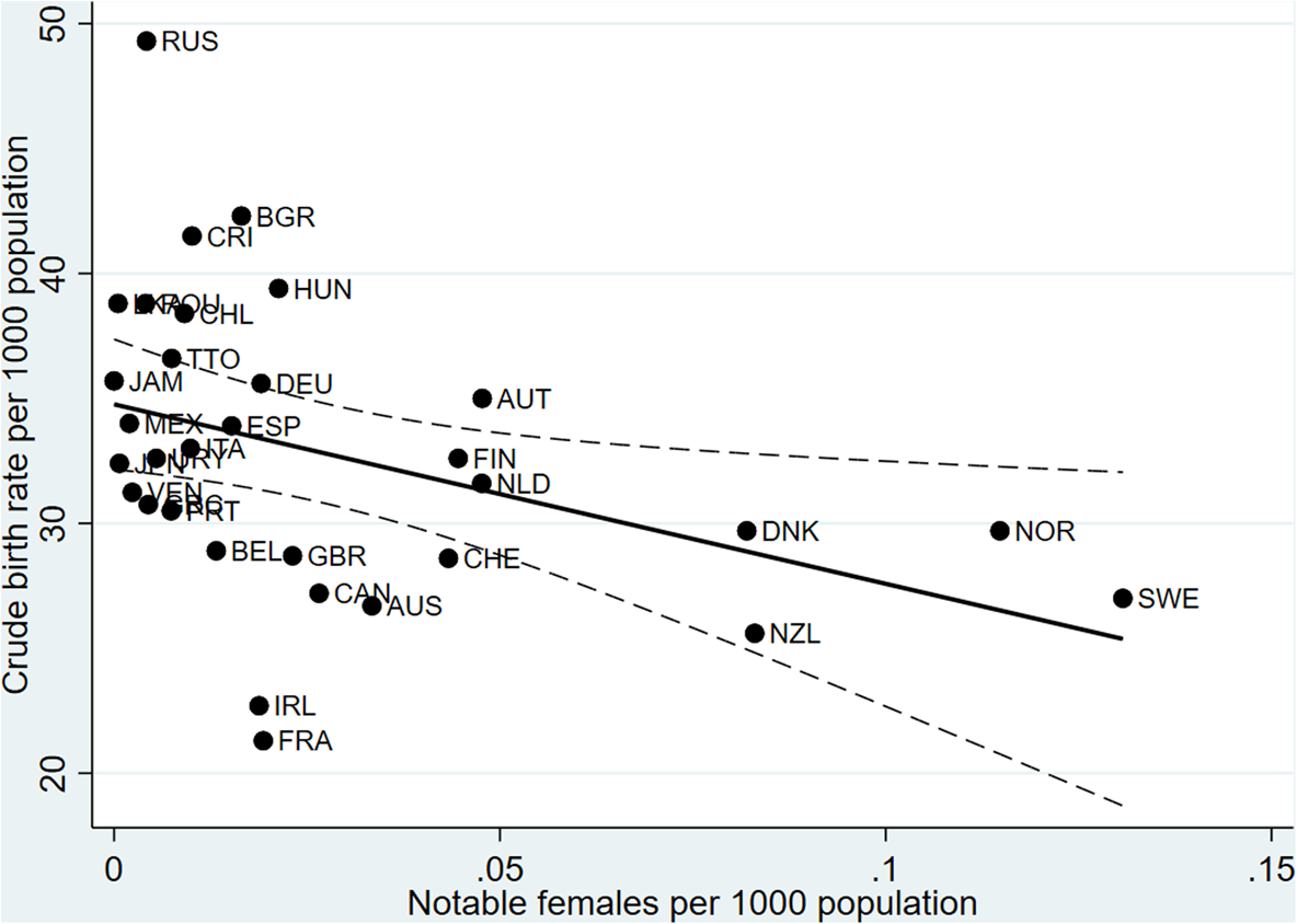
To study whether notable people impact fertility, we use crude birth rate per 1,000 population (variable br henceforth) as the dependent variable. We use the National Center for Health Statistics for the US birth rates, and Mitchell (Reference Mitchell2013)Footnote ⁷ for other countries. Finally, we end up with 3,769 non-missing birthrate observations, with data availability increasing from two countries (Norway and Sweden) in 1750, to 21 countries in 1870 when educational data become available, to 54 countries in 1950. Figure 1 correlates the number of notable women per capita and the birth rate in year 1900; a negative correlation is evident.

Figure 1.

Number of notable females per 1,000 population ($pcF$) and birth rate ($br$), year 1900. Dashed: 95% confidence interval.

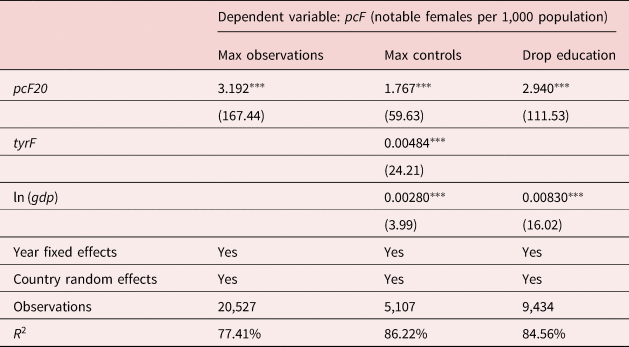
To account for possible endogeneity, that women with fewer children have more free time to study experiences of notable individuals and thus contribute to their fame, I instrument the influence variable $pcF_{it}$ in country $i$ and year $t$, by variable $pcF20_{it}$, defined as the number of notable females associated with country $i$, alive and aged 30+ in year $t-20$ but deceased by year $t$, per 1,000 population in year $t$. The identifying assumption is that a person in year $t$ cannot directly learn about a role model deceased by that year, only via a living intermediary role model.

Table 6 reports the results of the first stage of 2SLS, with varying sets of controls described above, with least controls corresponding to most time coverage. Three different regressions result in three versions of predicted values, labeled pc1, pc2, and pc3 respectively.

Table 6.

Influence on birthrate: first stage of 2SLS

t statistics in parentheses.

$^{\ast }$${\rm p}< 0.05$, $^{\ast \ast }$${\rm p}< 0.01$, $^{\ast \ast \ast }$${\rm p}< 0.001$.

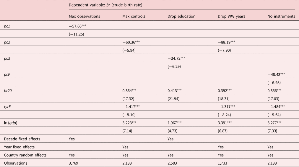
Besides the control variables described above, in the second stage of 2SLS I also include the birth rate 20 years earlier, $br20_{i, t} = br_{i, t-20}$, which may absorb many omitted controls. In the regressions excluding educational control tyrF, observations date back to 1750 when birth rate was measured for only two countries, hence year fixed effects cannot be used. In such regressions, I control for decade fixed effects instead.

Table 7 reports the results for various regression specifications. The fourth regression differs from the second by excluding World War years: although the global change in the birth rate during this period is captured by year fixed effects, World Wars could have affected different countries differently. The last regression shows the effect of non-instrumented measure of female influence. The influence of notable individuals, instrumented or not, has a strong and robust negative effect on birthrate. For example, the fourth regression estimates that each notable woman reduced the number of births in her country by 88.2 in every year from her age 30 until death. All control variables have expected sign, which reinforces credibility of the results.

Table 7.

Influence on birthrate: second stage of 2SLS

t statistics in parentheses.

$^{\ast }$${\rm p}< 0.05$, $^{\ast \ast }$${\rm p}< 0.01$, $^{\ast \ast \ast }$${\rm p}< 0.001.$

Table 8.

Concordance of Pantheon to NHIS 2004–2015 occupations

occfam is occupational fame (notable individuals per 1,000 employees).

This result confirms Hypothesis 3, that the presence of notable individuals reduces aggregate birth rate.