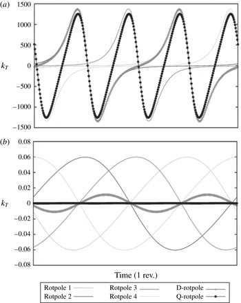
1 Introduction
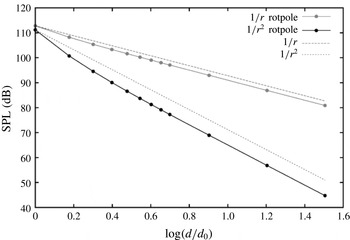
For a long time, the acoustic analysis of propulsion systems based on rotating blades has been the subject of many research activities all over the world. Nevertheless, since the publication of the Ffowcs Williams & Hawkings (Reference Ffowcs Williams and Hawkings1969) equation (FWH) and the first solving formulations developed by Farassat (Reference Farassat, Pegg and Hilton1975, Reference Farassat1981), attention has been exclusively paid to aeronautical devices. Both experimental data and numerical calculations soon demonstrated how in air, up to a blade tip Mach number approximately equal to
 $0.8$
, the acoustic field was dominated by noise generating mechanisms strictly related to the body surface. These mechanisms correspond to the surface terms of the governing equation and are known as thickness and loading noise components: the first is due to the fluid displacement caused by the body motion and depends on its shape, while the second is related to the loads occurring on the body surface. The computation of these terms is straightforward and hence turned out to be a very effective way to achieve a reliable assessment of the aeroacoustic field. Thus, while research moved on to the many complex problems related to the transonic and supersonic regimes, concerning the noise generated by shock waves and the possible multiple emissivity from supersonic sources (see, for example, Ianniello Reference Ianniello2007), the noise prediction from a subsonically rotating blade was considered to be a solved and closed matter, easily worked out with the computation of the surface integrals only. This historical excursus explains rather well why when researchers, in recent years, started to adopt the acoustic analogy for the hydroacoustic analysis of marine propellers, they felt empowered not to be worried at all about the volume quadrupole term (Seol et al.
Reference Seol, Jung, Suh and Lee2002, Reference Seol, Suh and Lee2005; Salvatore & Ianniello Reference Salvatore and Ianniello2003; Ye et al.
Reference Ye, Xiong, Xiao and Bi2010; Pan & Zhang Reference Pan and Zhang2013; Bagheri et al.
Reference Bagheri, Seif and Mehdigholi2014). On the other hand, to claim the rotational rate of such a device to be subsonic, sounds, more or less, like a euphemism. The sound speed underwater is approximately five times higher than in air and the body moves in a fluid a thousand times denser; consequently, the blades rotate very slowly and the same Mach number appears to be, at best, an irrelevant parameter. Not by chance, most of the few papers dealing with FWH-based underwater noise prediction use the Farassat linear formulae or, at best, the porous formulation (Di Francescantonio Reference Di Francescantonio1997; Brentner & Farassat Reference Brentner and Farassat1998), paying no particular attention to the contribution of nonlinear sources.
In addition to such ‘unquestionable’ dominance of the surface terms at subsonic speed, a rather popular tendency exists to associate the thickness and loading contributions to the well-known elemental sources, insomuch as the same components are more and more frequently labelled as some (not well-specified) monopole and dipole terms respectively. As is well known by aeroacousticians, these terms can actually be described by a suitable distribution of monopoles and dipoles, and some similarities immediately catch the eye: in the plane of rotation, for example, the acoustic field generated by a rotating body always exhibits a uniform (radial) directivity, very similar to the omnidirectional (spherical) directivity of a monopole, and the standard solution provides both the thickness and the loading noise in terms of two integral (far- and near-field) components, characterized by the well-known inverse and inverse-squared dependence on the source-observer distance. This is just the typical behaviour of monopoles and dipoles. Nevertheless, such a characterization of the FWH surface terms is more theoretical than practical, and it somehow masks the fundamental role played by the rotational speed; moreover, due to the known higher acoustic efficiency of monopoles and dipoles with respect to quadrupoles, it even reinforces the conviction about the dominance (at subsonic speed) of these two-dimensional (2D) terms with respect to the three-dimensional (3D) nonlinear one.
Unfortunately, the way the things are is very different. The usual subsonic operating conditions for an aeronautical device are very far from analogous configurations working underwater. In air, the rotational Mach number
 $M_{R}={\it\omega}R/c_{0}$
(where
 ${\it\omega}$
is the rotational rate,
 $R$
is the blade radius and
 $c_{0}$
is the sound speed in the undisturbed medium) varies from
 $0.3/0.5$
to values higher than unity; on the contrary, the same parameter for a marine propeller can easily approach
 $0.02$
or
 $0.01$
, then one or even two orders of magnitude lower than an aeronautical propeller or a helicopter rotor. At such low values of
 $M_{R}$
, the literature does not offer any stimulus for reflection and (to the best of the author’s knowledge) a detailed investigation on the behaviour of the FWH source terms has never been carried out. Within this context, many numerical simulations concerning different configurations (isolated propeller in a uniform flow, installed propeller operating in a hull wake and even some raw comparison with available full-scale ship data) and different FWH-based solving approaches (Farassat linear formulae, direct assessment of the quadrupole volume integrals, porous formulation) (Ianniello, Muscari & Di Mascio Reference Ianniello, Muscari and Di Mascio2011; Ianniello et al.
Reference Ianniello, Muscari and Di Mascio2013, Reference Ianniello, Muscari and Di Mascio2014a
,Reference Ianniello, Muscari and Di Mascio
b
; Ianniello Reference Ianniello2012; Ianniello & De Bernardis Reference Ianniello and De Bernardis2015) provide the precisely the same result: underwater, the thickness and loading noise components generated by a propeller vanish in a very limited region surrounding the body, so that, in spite of the low rotational speed, the hydroacoustic field ends up being dominated by the flow nonlinearities. At a first glance, the reasons for such an unexpected result, completely opposite to the behaviour of aeronautical devices, seemed to be ascribable to the structural and geometrical features of the blade and to the relevant nonlinear phenomena occurring underwater (Ianniello Reference Ianniello2014). A marine propeller has to move a huge mass of water: the blade has a very compact planform compared, for example, with a helicopter rotor, and is characterized by a low aspect ratio, a remarkable twist and a notable variation of chord and thickness along the span. The blades usually work in the highly turbulent flow generated by the hull and may give rise to different cavitation phenomena; nevertheless, even by accounting for a uniform inflow and non-cavitating conditions, the tip generates a vortical persisting wake, which develops downstream and inevitably suffers a breaking phase. All of these phenomena are nonlinear and accountable for noise. On the other hand, neither the geometrical features of the body nor the relevant nonlinear effects characterizing the underwater flow can explain the impressive and rapid annihilation of the surface terms. For this reason, the author decided to put aside any ‘consolidated knowledge’ coming from aeroacoustics and to refocus the attention on a basic fundamental problem: the acoustic behaviour of a rotating source. The result of this effort is quite interesting: it suggests an out-and-out role reversal between the surface and volume terms in the aeroacoustic and hydroacoustic analysis of rotating blades, ruled by the huge diversity of rotational speed of aeronautical and marine devices. In essence, this result has always been plain to see: it does not require any mathematical reformulation of the problem and can be explained in a very simple way, by analysing the behaviour of the thickness and loading integral kernels at operating conditions on which, by mere chance, attention has never been focused adequately.
The structure of the paper is as follows. Section 2 basically reviews the FWH equation and the integral linear formulation used throughout the paper, while § 3 proposes some food for thought concerning monopole, dipole and rotating sources, pointing out some relevant differences of the corresponding theoretical models. Section 4 introduces the rotpole and starts a long detailed analysis of the behaviour of a rotating source, through the definition of suitable kernel functions (§ 4.1), the discussion of the very-near-field effects (§ 4.2), the assessment of noise decay with the source-observer distance (§ 4.3) and the evaluation of noise directivity through the kernel function maps (§ 4.4). The significant effects of the interferences occurring for multiple rotating sources are discussed in § 5. In § 6, the analysis on kernel functions and a single source is applied to the FWH equation and a real blade, dealing with an instructive comparison between the thickness noise generated by a helicopter rotor and a marine propeller. The main results of the paper and their consequences for the hydroacoustic analysis of rotating blades are discussed in § 7. Finally, the conclusions are summarized in § 8.
2 The FWH equation and the standard solving formulations
The FWH equation represents a rearrangement of the fundamental conservation laws of mass and momentum into an inhomogeneous wave equation, written in terms of generalized functions
 $$\begin{eqnarray}\displaystyle \bar{\Box }^{2}p^{\prime }(\boldsymbol{x},t) & = & \displaystyle \frac{\bar{\partial }}{\partial t}\{[{\it\rho}_{0}v_{n}+{\it\rho}(u_{n}-v_{n})]{\it\delta}(f)\}-\frac{\bar{\partial }}{\partial x_{i}}\{[{\rm\Delta}\unicode[STIX]{x1D617}_{ij}\hat{n}_{j}+{\it\rho}u_{i}(u_{n}-v_{n})t]{\it\delta}(f)\}\nonumber\\ \displaystyle & & \displaystyle +\,\frac{\bar{\partial }^{2}}{\partial x_{i}\partial x_{j}}\{\unicode[STIX]{x1D61B}_{ij}H(f)\},\end{eqnarray}$$
where
 $p^{\prime }=c_{0}^{2}\tilde{{\it\rho}}$
,
 $\tilde{{\it\rho}}={\it\rho}-{\it\rho}_{0}$
being the density perturbation and
 ${\it\rho}_{0}$
,
 $c_{0}$
the density and sound speed respectively in the undisturbed medium; under the assumption of small perturbations (
 $\tilde{{\it\rho}}/{\it\rho}_{0}\ll 1$
),
 $p^{\prime }$
represents the acoustic pressure. The equation
 $f=0$
(where
 $f$
is the support of the Dirac
 ${\it\delta}(f)$
and the Heaviside
 $H(f)$
functions) indicates an arbitrary surface, whose choice heavily affects the physical meaning of the different terms. The D’Alembert operator is given by
 $\bar{\Box }^{2}=[1/c_{0}^{2}\bar{\partial }^{2}/\partial t^{2}]-\bar{{\rm\nabla}}^{2}$
, the Lighthill tensor is
 $\unicode[STIX]{x1D61B}_{ij}={\it\rho}u_{i}u_{j}+\unicode[STIX]{x1D617}_{ij}-c_{0}^{2}\tilde{{\it\rho}}{\it\delta}_{ij}$
and
 $\unicode[STIX]{x1D617}_{ij}$
represents the compressive stress tensor. The fluid and surface velocity components are indicated by
 $u_{i}$
and
 $v_{i}$
respectively, while
 $n$
denotes the projection along the outward normal to the surface. The presence of the Dirac and Heaviside functions points out the different nature of the source terms: two surface terms directly related to the effects of the discontinuity at
 $f=0$
in the flow field and a volume term accounting for all sources acting outside it. When
 $f=0$
coincides with the body surface
 $S$
, the impermeability condition
 $u_{n}=v_{n}$
simplifies (2.1), and the use of the Green function approach results in several different integral formulations, suitable for numerical implementation. Among these and for a long time, the formulation 1A developed by Farassat (Reference Farassat1981), has been the standard approach in most computer codes devoted to the aeroacoustic (linear) analysis of rotating blades. By accounting for an inertial frame of reference and under the assumptions of (i) fluid at rest, (ii) inviscid flow (which reduces the stress tensor to the scalar pressure field on the blade surface,
 $\unicode[STIX]{x1D617}_{ij}=(p-p_{0}){\it\delta}_{ij}=\tilde{p}{\it\delta}_{ij}$
) and (iii) isentropic transformations (for which the pressure–density relationship can be approximated by the linear term of its series expansion, i.e.
 $p^{\prime }=c_{0}^{2}\tilde{{\it\rho}}$
), the surface terms of (2.1) can be written in the following form:
 $$\begin{eqnarray}\displaystyle 4{\rm\pi}p_{T}(\boldsymbol{x},t) & = & \displaystyle \int _{S}\left[\frac{{\it\rho}_{0}\dot{(v_{n})}}{r|1-M_{r}|^{2}}+\frac{{\it\rho}_{0}v_{n}(\dot{M_{i}}\hat{r}_{i})}{r|1-M_{r}|^{3}}\right]_{{\it\tau}}\,\text{d}S\nonumber\\ \displaystyle & & \displaystyle +\,\int _{S}\left[\frac{{\it\rho}_{0}v_{n}c_{0}(M_{r}-M^{2})}{r^{2}|1-M_{r}|^{3}}\right]_{{\it\tau}}\,\text{d}S,\end{eqnarray}$$
 $$\begin{eqnarray}\displaystyle 4{\rm\pi}p_{L}(\boldsymbol{x},t) & = & \displaystyle \int _{S}\left[\frac{\dot{\tilde{p}}\cos {\it\theta}+\tilde{p}\dot{\hat{n}}_{i}\hat{r}_{i}}{c_{0}r|1-M_{r}|^{2}}+\frac{\tilde{p}\cos {\it\theta}(\dot{M_{i}}\hat{r}_{i})}{c_{0}r|1-M_{r}|^{3}}\right]_{{\it\tau}}\text{d}S\nonumber\\ \displaystyle & & \displaystyle +\,\int _{S}\left[\frac{\tilde{p}\cos {\it\theta}-\tilde{p}M_{n}}{r^{2}|1-M_{r}|^{2}}+\frac{\tilde{p}\cos {\it\theta}\left(M_{r}-M^{2}\right)}{r^{2}|1-M_{r}|^{3}}\right]_{{\it\tau}}\,\text{d}S,\end{eqnarray}$$
where, as already said,
 $S$
represents the surface of the body. In this case (and only in this case), the surface terms can be identified as the thickness and loading noise components, with their physical meaning related to the fluid displacement and surface loads due to the body motion, and are usually labelled as the ‘linear’ terms of the FWH equation. Here,
 $\tilde{p}$
is the gauge pressure on
 $S$
,
 $\hat{n}_{i}$
and
 $\hat{r}_{i}$
represent the components of the unit vectors along the outward normal (with respect to
 $S$
) and the radiation directions respectively,
 $\cos {\it\theta}=\hat{\boldsymbol{n}}\boldsymbol{\cdot }\hat{\boldsymbol{r}}$
, the subscript
 $r$
indicates the projection along
 $\boldsymbol{r}$
,
 $M=|\boldsymbol{v}|/c_{0}$
is the source Mach number and the dot over symbols indicates the time derivative. It is very important to note that all of the kernels are computed at the emission (retarded) time
 ${\it\tau}=t-r/c_{0}$
. The difference between
 ${\it\tau}$
and the corresponding observer time
 $t$
is called the compressibility delay: it represents a essential feature of the propagation mechanisms and points out that sound propagates in the medium at a finite speed. For our purposes, it is also important to note that each of the integral kernels exhibits a far-field and a near-field component, formally depending on the inverse and the inverse-squared of the source-observer distance
 $r=|\boldsymbol{x}(t)-\boldsymbol{y}({\it\tau})|$
. Henceforth, the phrase ‘FWH surface terms’ (unless otherwise specified) will explicitly refer to the two terms given by (2.2) and (2.3).
3 Thinking about monopoles, dipoles and rotating sources
As already said, the FWH thickness and loading noise components are often associated with some distribution of monopoles and dipoles respectively. Although theoretically correct, however, this correlation is certainly not the best way to describe the behaviour of the surface terms (2.2) and (2.3) when the body motion is rotational, and a different, likewise simple and more appropriate model could be used. As is well known, a monopole is a source radiating sound equally in all directions. It is often represented by a sphere pulsating at a fixed frequency
 $f_{0}$
, whose radius alternatively expands and contracts, thus generating a mass/volume flux and a spherical omnidirectional wave. Close to the sphere surface (in the near field), the fluid is accelerated from rest and its velocity is in phase quadrature with the pressure wave; very soon, however, this shift disappears and all around (in the far field) the noise decreases following the
 $1/r$
law (
 $r$
being the source-observer distance). This means a
 $6$
dB reduction at any doubling of the distance. A dipole is usually represented by two close-set monopoles of equal strength but with opposite sign, or, alternatively, a sphere oscillating along a prescribed axis. While one source expands, the other contracts, so that the net flux of mass is zero and the sound is generated by the net force on the fluid, that is a momentum flux. In this case, the sound field has a well-defined directionality (along the dipole axis), but the mutual interactions of the monopoles make the noise decay more pronounced in the proximity of the source; thus, in the near field the sound propagates according to the inverse-squared law
 $1/r^{2}$
, while maintaining the
 $1/r$
dependence in the far field. In other words, we can think of the near field like a sort of transition region where the different pressure disturbances progressively mix together, to achieve a single stabilized front radiating thereafter (in the far field) as a ‘plane’ wave. Qualitatively speaking, the near-field spatial dimension is estimated by the wavelength
 ${\it\lambda}$
of the resulting noise,
 $$\begin{eqnarray}O_{L_{nf}}=O({\it\lambda})=O(c_{0}T),\end{eqnarray}$$
where
 $T$
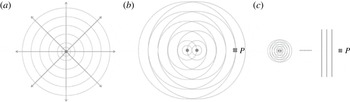
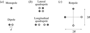
is the signal period. A sketch of these models is shown in figure 1. Figure 1(a) points out the omnidirectionality of the monopole source, while figure 1(b) and figure 1(c) give a schematic representation of the dipole near and far field respectively, as perceived at a fixed measurement point
 $P$
.
Schematic representation of the monopole and dipole elemental sources: (a) monopole, (b) dipole near field, (c) dipole far field.

Despite the usual and ideal modelling of the FWH surface terms through these elemental sources, the generating and propagating noise mechanisms concerning a rotating body can be, indeed, very different. The underlying problem is that the theoretical structure of the aforementioned monopole and dipole models is not sufficient to provide an immediate exhaustive description of the acoustic behaviour of a rotating source, and the missing, although essential, elements are the kinematic variables characterizing the rotational motion. First of all, it is interesting to note that even by accounting for a single rotating source, a sort of auto-interaction of kinematic nature occurs and gives rise to a transition region (that is, a near field) in the proximity of the source. In fact, at each position along the circular trajectory, the source induces a pressure disturbance in the surrounding fluid, but while the whole revolution is completed these disturbances interact with each other in a way strictly dependent on the rotational speed
 ${\it\omega}$
. Intuitively, the interaction is more pronounced at smaller values of
 ${\it\omega}$
, since the shift between the subsequent disturbances increases. The period appearing in the qualitative assessment of near-field size now corresponds to the revolution period
 $T=2{\rm\pi}/{\it\omega}$
, and (3.1) can be written as
 $$\begin{eqnarray}O_{L_{nf}}=O\left(\frac{2{\rm\pi}c_{0}}{{\it\omega}}\right)=O\left(\frac{2{\rm\pi}R}{M_{R}}\right).\end{eqnarray}$$
This relation states that, for a fixed value
 $R$
of the radius of motion, a source rotating at
 $M_{R}=0.01$
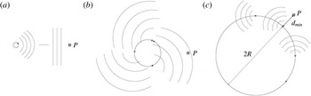
can give rise to a near field 100 times larger than the near field of the same source rotating at sonic speed. How does the noise behave in this (eventually very large) region? Some suggestions are provided in figure 2, depicting an observer at different distances from the source. The far field (figure 2
a) can be still recognized as the region where the noise decreases according to the
 $1/r$
law and the observer perceives the rotating source as a point (compact) source. The distance
 $d$
between this observer and the rotation axis is larger than
 $2R$
(the size of the circular trajectory), but the far-field size strongly depends on
 ${\it\omega}$
: the higher the rotational speed, the more compact the source and, consequently, the closer to the source the far field is. When
 $d$
has a value comparable to
 $2R$
(figure 2
b), the observer is in a region characterized by the interactions between the pressure disturbances induced by the motion; then, it is reasonable to identify this region as the near field and, like a dipole, to expect a noise decay governed by the inverse-squared law
 $1/r^{2}$
. Nevertheless, a further reduction of the distance
 $d$
(figure 2
c) gives rise to a rather anomalous situation.
Noise propagation mechanisms related to a rotating source: (a)
 $d\gg 2R$
, far field, (b)
 $d\approx O(2R)$
, near field, (c)
 $d_{min}<2R$
, very near field.

Within a revolution period, in fact, the observer experiences both
 $d_{min}<2R$
and
 $d_{max}=d_{min}+2R>2R$
, thus very close to the source (which, moreover, corresponds to the numerical singularity
 $r=0$
) and in a position previously identified as a near field. Still, the way in which the sound reaches the observer in such a very near field is strictly related to the rotational motion and, as for the near field of a dipole, we could expect this region to widen with decreasing rate. This configuration, however, points out very well that the ‘structure’ of a rotating source is deeply different with respect to the simple monopole and dipole models depicted in figure 1, and suggests that the whole aforementioned transition region may extend much further out. Furthermore, according to our description of the near field, it is quite hard to believe that, approaching the blade, the noise could always decrease following the
 $1/r^{2}$
law for any value of
 ${\it\omega}$
. Thus, the question is how the noise actually behaves in the near field and how this behaviour is affected by the rotational speed. Unfortunately, in the past, research was always focused on the effects of an aeronautical high
 $M_{R}$
in the far field, while it substantially ignored the effects of a marine low
 $M_{R}$
in the near field. The literature offers many papers concerning possible analytic solutions for a rotating source, in both the time and frequency domains (Morfey & Tanna Reference Morfey and Tanna1971; Tanna & Morfey Reference Tanna and Morfey1971; Poletti Reference Poletti2010; Poletti & Teal Reference Poletti and Teal2011; Tang et al.
Reference Tang, Qi and Mao2013). Most of them, however, refer to a monopole source (equipped with an auto-pulsating frequency
 $f_{0}$
), are focused on high values of the rotational speed and, above all, are based on rather complex mathematical manipulations, which make the physics of the underlying phenomena difficult to understand. For this reason, our investigations will be carried out through a practical approach, by directly investigating the behaviour of the FWH surface terms for a single rotating source.
4 The rotpole
In order to characterize the acoustic behaviour of a rotating source and to analyse its own features through the Farassat formulation 1A, it is useful to think of a new elemental source: the rotpole. Like the well-known models concerning the elemental sources, the rotpole (
 $\mathscr{R}$
) can be represented by a small sphere of radius
 $a$
, located at a distance
 $R\gg a$
from the
 $z$
axis of a Cartesian frame of reference
 $O(xyz)$
and rotating counterclockwise around it (that is, in the
 $xy$
disk plane) at a fixed rotational speed
 ${\it\omega}$
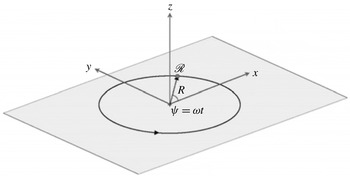
. The rotpole, however, is rigid: it has no pulsating motion and thus is able to generate sound only by virtue of its own rotation (then through the displacement of the surrounding fluid) and/or an associated force rotating with it. A sketch of this simple model is shown in figure 3. The main aim of our analysis is to understand how the kinematics of the source affects the sound propagation and, then, the acoustic integrals of (2.2) and (2.3). In particular, the interest is here focused on noise decay (moving far from the source) as a function of the rotational speed.
The rotpole
 $\mathscr{R}$
.

It is worth mentioning that this kind of analysis could be performed by modelling the rotpole by a spherical mesh and computing, at different points, the thickness and (with
 $\tilde{p}$
available) loading noise components. Nevertheless, in order to get to the heart of the problem, we identify the rotpole with a point source and, for each surface term, analyse the behaviour of a kernel function accounting for the only dependence of the corresponding integral on kinematic parameters. It is fundamental to stress that, in this way, the calculations are carried out analytically: they do not require any numerical validation and are free from any link to the shape of the body source or the corresponding aero/hydrodynamic loads. In the following, unless otherwise specified, the calculations will refer to water; thus, the sound speed
 $c_{0}$
is set to
 $1500~\text{m}~\text{s}^{-1}$
and the reference pressure for the computation of the sound pressure level (SPL) in dB is
 $p_{ref}=10^{-6}$
Pa (the usual reference value underwater).
4.1 The rotpole kernel functions
The rotpole kernel functions, indicated by
 $k(\cdot )$
, may be considered as a practical way to describe the acoustic behaviour of a rotating source and, at the same time, to achieve a deep understanding of the general behaviour of the FWH surface terms. First of all, as we refer to a point source, the coordinates of the rotpole and their subsequent time derivatives (see figure 3) can be simply written in the following form:
 $$\begin{eqnarray}\displaystyle & \displaystyle \mathscr{R}\equiv (R\cos {\it\omega}t,R\sin {\it\omega}t,0), & \displaystyle\end{eqnarray}$$
 $$\begin{eqnarray}\displaystyle & \displaystyle \boldsymbol{v}\equiv (-{\it\omega}R\sin {\it\omega}t,+{\it\omega}R\cos {\it\omega}t,0), & \displaystyle\end{eqnarray}$$
 $$\begin{eqnarray}\displaystyle & \displaystyle \dot{\boldsymbol{v}}\equiv (-{\it\omega}^{2}R\cos {\it\omega}t,-{\it\omega}^{2}R\sin {\it\omega}t,0). & \displaystyle\end{eqnarray}$$
 $k(\cdot )$
with the corresponding integral kernels, rid of all terms not directly accounting for the kinematic variables of interest. In particular, we assume here that the strength of the source terms (expressed by
 $({\it\rho}_{0}\dot{v_{n}})$
,
 ${\it\rho}_{0}v_{n}$
for thickness and
 $\dot{\tilde{p}}$
,
 $\tilde{p}$
for loading components) is responsible of the SPL value at any point, but it does not affect the relationship between the source kinematics and noise propagation at all. Thus, in our definition of the kernel functions, the abovementioned strength is simply ignored (or, in other words, is set to 1). The author is well aware of the poor mathematical strictness of this approach, but its practical advantages will soon be clear. On the other hand, the attention here is not focused on the prediction of noise (it would be quite bizarre to compute a thickness noise from a point source), but rather on the numerical trend of the acoustic integrals, as ruled by the rotational motion. In any case, it will be shown later that the analytical results provided by such a practical approach exactly match the numerical solutions provided by formulation 1A. With this explanation and the previously mentioned assumption concerning
 $({\it\rho}_{0}\dot{v_{n}})$
,
 ${\it\rho}_{0}v_{n},\dot{\tilde{p}}$
and
 $\tilde{p}$
, the rotpole kernel functions can be written in the following form:
 $$\begin{eqnarray}k_{T}({\it\omega},r,c_{0})=k_{T}^{F}+k_{T}^{N}=\left\{\frac{1}{r}\left[\frac{{\dot{M}}_{i}\hat{r}_{i}}{|1-M_{r}|^{3}}\right]\right\}^{F}+\left\{\frac{1}{r^{2}}\left[\frac{c_{0}\left(M_{r}-M^{2}\right)}{|1-M_{r}|^{3}}\right]\right\}^{N},\end{eqnarray}$$
 $$\begin{eqnarray}\displaystyle k_{L}({\it\omega},r,c_{0},\hat{\boldsymbol{n}}) & = & \displaystyle k_{L}^{F}+k_{L}^{N}=\left\{\frac{1}{r}\left[\frac{\cos {\it\theta}}{c_{0}|1-M_{r}|^{2}}+\frac{\dot{\hat{n}}_{i}\hat{r}_{i}}{c_{0}|1-M_{r}|^{2}}+\frac{{\dot{M}}_{i}\hat{r}_{i}\cos {\it\theta}}{c_{0}|1-M_{r}|^{3}}\right]\right\}^{F}\nonumber\\ \displaystyle & & \displaystyle +\left\{\frac{1}{r^{2}}\left[\frac{\cos {\it\theta}-M_{n}}{|1-M_{r}|^{2}}+\frac{\cos {\it\theta}\left(M_{r}-M^{2}\right)}{|1-M_{r}|^{3}}\right]\right\}^{N},\end{eqnarray}$$
where the superscripts
 $F$
and
 $N$
emphasize the distinction between the far- and near-field components, depending on
 $1/r$
and
 $1/r^{2}$
respectively. First of all, note the absence of the term
 $\dot{(v_{n})}$
of (2.2) in the definition (4.2) of
 $k_{T}^{F}$
. Actually, many of the integral kernels exhibit the unit vector
 $\hat{\boldsymbol{n}}$
, locally defining the outward normal direction with respect to the integration domain and rigidly attached to it. By assuming a generic triad of components in a frame of reference in-built with the point source
 $\hat{\boldsymbol{n}}|^{{\it\eta}}=(n_{1},n_{2},n_{3})$
, satisfying the condition
 $(n_{1}^{2}+n_{2}^{2}+n_{3}^{3})^{1/2}=1$
, the quantities
 $\hat{n}_{i}$
appearing in the kernel functions may be obtained by the simple relation
 $$\begin{eqnarray}\hat{\boldsymbol{n}}=\left[\begin{array}{@{}c@{}}n_{x}\\ n_{y}\\ n_{z}\end{array}\right]=\unicode[STIX]{x1D64F}\;\hat{\boldsymbol{n}}|^{{\it\eta}}=\left[\begin{array}{@{}ccc@{}}\cos {\it\omega}t & -\sin {\it\omega}t & 0\\ \sin {\it\omega}t & \cos {\it\omega}t & 0\\ 0 & 0 & 1\end{array}\right]\left[\begin{array}{@{}c@{}}n_{1}\\ n_{2}\\ n_{3}\end{array}\right],\end{eqnarray}$$
that is
 $$\begin{eqnarray}\hat{\boldsymbol{n}}=\left(n_{1}\cos {\it\omega}t-n_{2}\sin {\it\omega}t,n_{1}\sin {\it\omega}t+n_{2}\cos {\it\omega}t,n_{3}\right),\end{eqnarray}$$
where
 $\unicode[STIX]{x1D64F}$
is the counterclockwise rotation matrix. In our analysis concerning a point source, as well as in the case of a rigid body for which the only time dependence of the unit vector
 $\hat{\boldsymbol{n}}$
is related to the rotational motion, (4.5) gives
 $$\begin{eqnarray}\dot{\hat{\boldsymbol{n}}}=\left[-{\it\omega}\left(n_{1}\sin {\it\omega}t+n_{2}\cos {\it\omega}t\right),{\it\omega}\left(n_{1}\cos {\it\omega}t-n_{2}\sin {\it\omega}t\right),0\right],\end{eqnarray}$$
and it is easy to verify (by (4.1b
), (4.1c
), (4.5) and (4.6)) that
 $\dot{(v_{n})}=\dot{v}_{i}\hat{n}_{i}+v_{i}\dot{\hat{n}}_{i}$
is equal to zero. In other words, the local shape of a (rigid) body characterizes the strength of the thickness component, but it does not affect how the thickness noise propagates in the field at all. On the contrary, the presence of
 $\cos {\it\theta}$
,
 $\dot{\hat{n}}_{i}\hat{r}_{i}$
and
 $M_{n}$
forces inclusion of the unit normal vector in the list of the independent variables for
 $k_{L}$
and suggests an actual dependence of the loading noise propagation on the local shape of the body. The effects of
 $\hat{\boldsymbol{n}}$
on the rotpole loading kernel function will be discussed in § 4.3.2. Other interesting features of
 $k_{L}$
lie in the presence of the
 $1/c_{0}$
shrinking factor affecting all terms of
 $k_{L}^{F}$
and, above all, the nature of the first two ratios, exhibiting the same denominator, but intentionally written in a separate way. The first term (with
 $\cos {\it\theta}$
in the numerator), in fact, is the only one corresponding to a different source strength (
 $\dot{\tilde{p}}$
, as opposed to
 $\tilde{p}$
); then, this term does not scale as all the other ones and can significantly alter the weight of the far-field component in the assessment of the overall behaviour of
 $k_{L}$
. This unsteady part of the loading kernel function could be simply removed by assuming a steady-state condition for the rotpole (like a point of a helicopter rotor in hover or a marine propeller in a uniform flow, for which
 $\dot{\tilde{p}}=0$
), but it is important to take it into account since it is known (at least in aeroacoustics) that its contribution can be dominant just at low blade rotational velocities. Then, for completeness, we preserve it in the definition of (4.3) and will deal with its possible effects in the following. At this point, it is fundamental to note that, for fixed
 $c_{0}$
,
 ${\it\omega}$
and a measurement point
 $P(x_{P},y_{P},z_{P})$
, the expressions
 $$\begin{eqnarray}\displaystyle & \displaystyle r=|\boldsymbol{r}|=\sqrt{\left(x_{P}-R\cos {\it\omega}t\right)^{2}+\left(y_{P}-R\sin {\it\omega}t\right)^{2}+z_{P}^{2}}, & \displaystyle\end{eqnarray}$$
 $$\begin{eqnarray}\displaystyle & \displaystyle M_{r}=M_{i}\hat{r}_{i}=\frac{v_{i}r_{i}}{c_{0}r}=\frac{{\it\omega}R}{c_{0}r}\left[-x_{P}\sin {\it\omega}t+y_{P}\cos {\it\omega}t\right], & \displaystyle\end{eqnarray}$$
 $$\begin{eqnarray}\displaystyle & \displaystyle {\dot{M}}_{i}\hat{r}_{i}=\frac{\dot{v}_{i}r_{i}}{c_{0}r}=\frac{1}{c_{0}r}\left[{\it\omega}^{2}R^{2}-{\it\omega}^{2}R\left(x_{P}\cos {\it\omega}t+y_{P}\sin {\it\omega}t\right)\right], & \displaystyle\end{eqnarray}$$
 $$\begin{eqnarray}\displaystyle & \displaystyle M_{n}=\left(\frac{{\it\omega}R}{c_{0}}n_{2}\right), & \displaystyle\end{eqnarray}$$
 $$\begin{eqnarray}\displaystyle & \displaystyle M^{2}=\left(\frac{{\it\omega}R}{c_{0}}\right)^{2}, & \displaystyle\end{eqnarray}$$
 $$\begin{eqnarray}\displaystyle & \displaystyle \cos {\it\theta}=\hat{n}_{i}\hat{r}_{i}=\frac{1}{r}\left[\left(x_{P}n_{1}+y_{P}n_{2}\right)\cos {\it\omega}t+\left(x_{P}n_{2}-y_{P}n_{1}\right)\sin {\it\omega}t-Rn_{1}+z_{P}n_{3}\right], & \displaystyle\end{eqnarray}$$
 $$\begin{eqnarray}\displaystyle & \displaystyle \dot{\hat{n}}_{i}\hat{r}_{i}=\frac{1}{r}\left[-{\it\omega}\left(x_{P}n_{1}+y_{P}n_{2}\right)\sin {\it\omega}t-{\it\omega}\left(x_{P}n_{2}-y_{P}n_{1}\right)\cos {\it\omega}t-{\it\omega}Rn_{2}\right] & \displaystyle\end{eqnarray}$$
 $T=2{\rm\pi}/{\it\omega}$
and turned into the frequency domain by a discrete Fourier transform (DFT) to evaluate the corresponding SPL at
 $P$
. Then, by changing the measurement point, the SPL decay for
 $k_{T}$
and
 $k_{L}$
can be determined as a function of
 $r$
. In the following, the decay curves will always be compared with the
 $1/r^{n}$
‘reference laws’, expressed by the geometric relationship
 $$\begin{eqnarray}\text{SPL}=\text{SPL}_{0}-20\log \left(\frac{d}{d_{0}}\right)^{n},\end{eqnarray}$$
where SPL and
 $\text{SPL}_{0}$
represent the pressure levels at two (aligned) points located at distances
 $d$
and
 $d_{0}$
respectively from the rotation axis. In particular,
 $n=1$
and
 $n=2$
define the well-known inverse (
 $1/r$
) and inverse-squared (
 $1/r^{2}$
) laws, corresponding to an SPL decrease of
 $6$
dB and
 $12$
dB at doubled (
 $d=2d_{0}$
) distances.
4.2 Very-near-field effects
Before starting the analysis of noise decay, it is interesting to show how the behaviour of the acoustic integrals may strictly depend on the rotational motion and, hence, require a good deal of caution. As already mentioned in the previous section, a measurement point close to the rotpole (in a region we called the very near field) experiences a remarkable variation of
 $r$
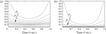
within the revolution period. Figure 4 shows the rotpole
 $1/r$
(a) and
 $1/r^{2}$
(b) curves, computed by (4.7a
) in one revolution period, at 13 subsequent points
 $P_{i}$
located along the
 $x$
axis (see figure 3);
 $R$
is set to
 $1~\text{m}$
and the distance from the rotation axis starts from
 $x_{P_{1}}=2~\text{m}$
, increases by
 $1~\text{m}$
up to the tenth point (
 $x_{P_{i}}=x_{P_{i-1}}+1,i=2,3\ldots 10$
) and then is set to 16, 32 and 64 m. The greater the distance, the more pressed towards the
 $x$
axis the curves are, especially, of course, for
 $n=2$
.
The rotpole (a)
 $1/r$
and (b)
 $(1/r^{2})$
functions within a revolution period, at 13 points along the
 $x$
axis. The point
 $P_{1}$
is located at only 2 m from the origin.

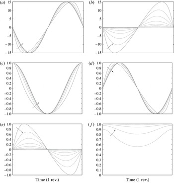
However, at points closer to the source, the functions exhibit a notable variation during the revolution; in particular,
 $P_{1}$
experiences a minimum distance from the rotpole
 $r_{min}=1~\text{m}$
and a maximum one
 $r_{max}=3~\text{m}$
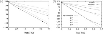
. The question is: what is, in this case, the behaviour (in dB) of the
 $1/r$
and
 $1/r^{2}$
functions? As is well known, the inverse law
 $1/r$
provides a decrease of
 $6$
dB at each doubling of the distance. Nevertheless, this is true for a fixed distance, while, in our case,
 $r$
is a function of time, and the more the point approaches the source, the more it ‘suffers’ this time dependence. Figure 5 shows the
 $1/r$
and
 $1/r^{2}$
functions of the rotpole, as computed in dB at the prescribed measurement points (with
 $z_{P}=0$
). Both of the curves exhibit an evident discrepancy with respect to the reference decay laws, and in the region between points
 $P_{1}$
and
 $P_{2}$
the SPL drop appears to be steeper. From a numerical point of view, the reason for this behaviour is clear: when
 $O(x_{P},y_{P})\approx O(R)$
, the two terms in brackets of (4.7a
) give rise to a non-negligible fluctuation of
 $r$
and the curves do not follow the standard decay. By increasing the distance (and then
 $O(x_{P},y_{P})$
), the weight of the oscillating terms
 $R\cos {\it\omega}t$
and
 $R\sin {\it\omega}t$
in (4.7a
) reduces and the curves soon align to the reference laws. At a first glance, the very-near-field effects can appear to not be so relevant: the gap between the
 $1/r$
curves soon settles on approximately
 $1.8$
dB and even reduces by moving out of the disk plane, where the fluctuating terms are also contrasted by the coordinate
 $z_{P}\neq 0$
; nevertheless, the gap rises up to
 $6.2$
dB for
 $1/r^{2}$
and can become significant (as will be shown later) for higher values of
 $n$
. In any case, these results reveal in advance how the behaviour of the acoustic kernels may be intimately related to the kinematics of the rotational motion.


4.3 Noise decay
At this stage, let us start our analysis on the relationship between the rotpole rotational speed and the kernel function decay in the field. To this aim, two measurement lines will be taken into account throughout this section: line
 $A$
corresponds to the
 $x$
axis, so as to assess the noise propagation in the plane of motion, while line
 $B$
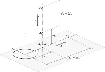
is orthogonal to the disk plane and allows us to evaluate the behaviour of the numerical solution in a very important direction (downstream of the propeller, where the blade tip vortex spreads underwater). The rotpole is always located at a distance
 $R=1~\text{m}$
from the rotation axis, corresponding to the
 $z$
axis of the reference. Each line includes 10 ordered points, starting from the disk plane points
 $A_{1}\equiv B_{1}\equiv (2,0,0)$
; along line
 $A$
, the distance of each point from the origin is doubled, while along line
 $B$
, the doubling refers to the distance from the disk plane. The coordinates of all measurement points are listed in table 1, for clarity, with
 $y_{A_{i}}=z_{A_{i}}=y_{B_{i}}=0$
and
 $x_{B_{i}}=2$
for
 $i=1,2\ldots 10$
, and a sketch of the measurement lines is depicted in figure 6.
Coordinates of measurement points along lines
 $A$
and
 $B$
.

Sketch of the measurement lines
 $A$
and
 $B$
.

4.3.1 Thickness kernel function
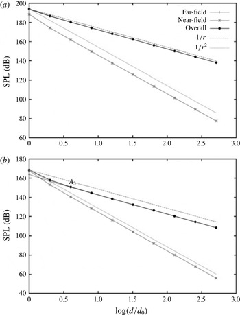
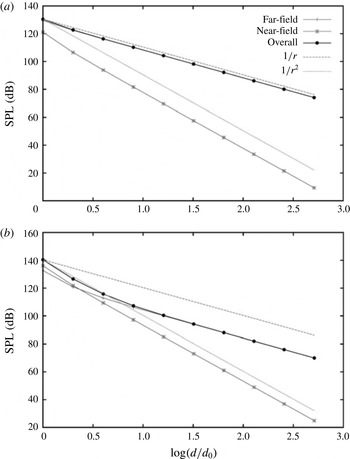
The thickness kernel functions in dB at points
 $A_{i}$
for a rotpole at rotational Mach numbers of
 $M_{R}=0.8$
and
 $M_{R}=0.4$
are shown in figure 7. Each panel shows the far- and near-field components separately, the overall SPL for
 $k_{T}$
and the reference decay laws of interest. At
 $M_{R}=0.8$
(figure 7
a), the far-field component is dominant: it fully overlaps the overall SPL and is very close to the
 $1/r$
reference law, although exhibiting a small gap due to the very-near-field effects, here affecting the region between points
 $A_{1}$
and
 $A_{2}$
. In practice, at this value of the rotational speed, the near-field component follows, as expected, the
 $1/r^{2}$
law, but it does not contribute at all to the resulting SPL, and the noise level decays according to
 $1/r$
everywhere in the field. By halving the rotational speed (
 $M_{R}=0.4$
, figure 7
b), the near-field component becomes significant in the proximity of the source. There, in fact, the overall SPL at
 $A_{1}$
is dictated by the
 $k_{T}^{N}$
component and the resulting decay curve clearly appears as the envelope of the two contributions. Nevertheless, the far-field component soon gets the upper hand, and at point
 $A_{3}$
(at only
 $8~\text{m}$
from the origin) the overall decay is already realigned to the
 $1/r$
reference line. Then, in spite of a notable drop of the noise level due to the lower rotational speed (compared with
 $M_{R}=0.8$
, at
 $A_{1}$
the overall SPL reduces from 194 to 168 dB), there is no remarkable qualitative change of the acoustic field, which remains deeply characterized by the
 $1/r$
law. It is worth pointing out that the rotational Mach numbers taken into account here represent two standard values for aeronautical devices, and our analysis of noise propagation in the field, based on the kernel functions, does not add any new information on the well-known behaviour of the thickness noise component: as expected, within this range of the rotational velocity and in the plane of motion, this surface term behaves in a way very similar to a monopole. Nevertheless, by decreasing the blade rate, the general trend of the decay curves progressively changes.
Rotpole thickness kernel function decay in the disk plane (measurement line
 $A$
) at
 $M_{R}=0.8$
(a) and
 $M_{R}=0.4$
(b).

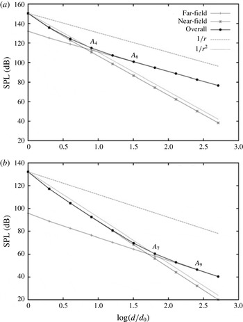
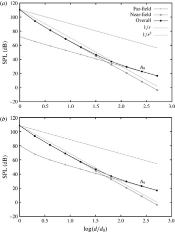
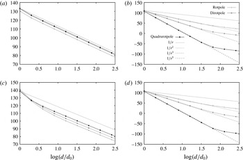
Figure 8(a) shows the rotpole
 $k_{T}$
function at
 $M_{R}=0.08$
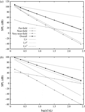
, that is ten times slower with respect to the first test case. At this value of the velocity, as suggested by relation (3.2), the near field is more extended and the
 $k_{T}^{N}$
component dominates up to point
 $A_{4}$
, while the overall level starts to follow the inverse law only at point
 $A_{6}$
, at a distance of 64 m from the origin. This situation corresponds to a more considerable change of the acoustic field, with a constant gap of approximately
 $20$
dB between the reference curve
 $1/r$
and the thickness kernel function in the far field. However, at
 $M_{R}=0.01$
, finally representing a more realistic value for a marine propeller, the SPL drop becomes really significant. The results are shown in figure 8(b). Here, the dominance of the near-field component covers a distance from the origin up to 128 m (point
 $A_{7}$
), and the governing
 $1/r^{2}$
decay law postpones the alignment of the overall SPL to the
 $1/r$
law at point
 $A_{9}$
, located half a kilometre from the rotpole. Furthermore, at such a long distance from the source, the noise level has already experienced a drop of approximately
 $40$
dB with respect to the value dictated by (4.8) with
 $n=1$
.
Rotpole thickness kernel function decay in the disk plane (measurement line
 $A$
) at
 $M_{R}=0.08$
(a) and
 $M_{R}=0.01$
(b).

Due to the way in which we have defined the kernel functions, this fall of the SPL represents an intrinsic feature of the rotpole behaviour, just ruled by the kinematics of the rotational motion and, in particular, the low value of
 $M_{R}$
. Moving out of the disk plane (
 $z_{P}\neq 0$
), the behaviour of the kernel function becomes more interesting.
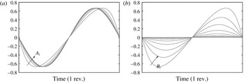
Plot of
 $M_{r}$
at points
 $A_{i}$
(disk plane, (a)) and
 $B_{i}$
(out of the disk plane, (b)).

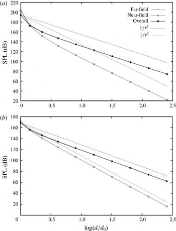
Rotpole thickness kernel function decay out of the disk plane (measurement line
 $B$
) at
 $M_{R}=0.8$
(a) and
 $M_{R}=0.4$
(b).

The far- and near-field components of (4.2) include the terms
 ${\dot{M}}_{i}\hat{r}_{i}$
and
 $M_{r}$
(expressions (4.7b
) and (4.7c
)). Within the disk plane, these terms exhibit a dependence on
 $r$
strictly related to the rotational motion, and the
 $r$
appearing in the denominator of (4.7a
) (where now
 $z_{P}=0$
) is fully balanced by the terms in brackets in the corresponding numerator; thus, both
 ${\dot{M}}_{i}\hat{r}_{i}$
and
 $M_{r}$
obviously exhibit a fluctuating waveform in the revolution period, but do not change with
 $r$
along the measurement line
 $A$
.
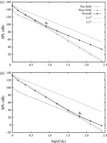
Rotpole thickness kernel function decay out of the disk plane (measurement line
 $B$
) at
 $M_{R}=0.08$
(a) and
 $M_{R}=0.01$
(b).

On the contrary, out of the disk plane
 $z_{P}$
is not zero and expressions (4.7b
) and (4.7c
) reveal, due to
 $r$
in the denominator, a dependence on the inverse law for
 ${\dot{M}}_{i}\hat{r}_{i}$
and
 $M_{r}$
. Such a behaviour, of course, comes from the two-dimensional nature of the rotational motion of the source and can be easily verified by numerically solving the previously mentioned equations. This solution is depicted in figure 9, showing the
 $M_{r}$
term at points
 $A_{i}$
(a) and
 $B_{i}$
(b), by increasing
 $i=1,2\ldots \,$
in one period. The additional
 $1/r$
dependence of
 ${\dot{M}}_{i}\hat{r}_{i}$
and
 $M_{r}$
suggests that (4.2) should be rewritten in the form
 $$\begin{eqnarray}k_{T}({\it\omega},r,c_{0})=\left\{\frac{1}{r^{2}}\left[\frac{{\dot{M}}_{i}r_{i}-c_{0}M^{2}}{|1-M_{r}|^{3}}\right]\right\}^{F}+\left\{\frac{1}{r^{3}}\left[\frac{v_{i}r_{i}}{|1-M_{r}|^{3}}\right]\right\}^{N},\end{eqnarray}$$
so as to point out that the kernel function
 $k_{T}$
is now characterized by a far-field term depending on
 $1/r^{2}$
and a near-field one depending on
 $1/r^{3}$
. In other words, out of the rotational plane the acoustic integrals combine in a different way to provide the far- and near-field components, and the thickness source term never behaves like a monopole (ruled by the inverse law), not even in the far field. This fact has important consequences, especially at a low rotational speed. (It should be noted that
 $M_{r}$
also appears in the denominator of all integral kernels, but in a way that does not alter the
 $r$
dependence of the kernel itself. The Doppler factor
 $|1-M_{r}|$
, in fact, oscillates as in figure 9(a) in the plane of motion, while out of that plane it simply tends to 1, when
 $M_{r}\rightarrow 0$
by increasing
 $r$
.) Figure 10 shows the thickness kernel functions on measurement line
 $B$
for a rotpole at
 $M_{R}=0.8$
(a) and
 $M_{R}=0.4$
(b). The curves confirm the new dependence of
 $k_{T}^{F}$
and
 $k_{T}^{N}$
on
 $r$
and that, as for points
 $A_{i}$
at such values of the rotational speed, the near-field component does not provide any significant contribution to the overall SPL. In essence, the
 $k_{T}$
function varies as
 $1/r^{2}$
in the whole field, thus confirming, as expected, that the thickness term decreases more rapidly than in the disk plane. Nevertheless, once again, by reducing the rotational speed to more realistic values for marine devices, the situation changes significantly. Figure 11 depicts the
 $k_{T}$
decay curves along line
 $B$
, at
 $M_{R}=0.08$
(a) and
 $M_{R}=0.01$
(b). At these values of the Mach number, the near-field size progressively increases and the overall SPL decay is dominated by
 $k_{T}^{N}$
in a large part of the field. In particular, at
 $M_{R}=0.08$
the near-field component governs the overall SPL (thus imposing a decay ruled by the
 $1/r^{3}$
law) up to point
 $B_{5}$
, while at
 $M_{R}=0.01$
the far-field component regains a relevant role only at point
 $B_{8}$
, at 128 m from the disk plane. However, at such a blade rate, by the time the overall SPL realigns to the
 $1/r^{2}$
law, the kernel function
 $k_{T}$
is rapidly going to zero.
4.3.2 Loading kernel function
The behaviour of the kernel function for the loading source term exhibits many analogies with
 $k_{T}$
, since the parameters governing the relationship between the noise decay and the source kinematics are essentially the same. Nevertheless,
 $k_{L}$
includes a strict dependence on the unit normal vector
 $\hat{\boldsymbol{n}}$
and the additional elements
 $M_{n}=v_{i}\hat{n}_{i}/c_{0}$
,
 $\cos {\it\theta}=\hat{n}_{i}\hat{r}_{i}$
and
 $\dot{\hat{n}}_{i}\hat{r}_{i}$
, which make the situation a little more complicated. The projection of the Mach number along the normal direction
 $M_{n}$
does not include any reference to the source-observer distance; it only depends on the local shape of the body source and the rotational speed, so it does not affect the
 $r$
dependence of the kernel function on its own. On the contrary,
 $\cos {\it\theta}$
and
 $\dot{\hat{n}}_{i}\hat{r}_{i}$
can behave in a manner very similar to
 ${\dot{M}}_{i}\hat{r}_{i}$
and
 $M_{r}$
, and, then, alter the
 $k_{L}$
decay with the
 $r$
distance. In order to analyse the possible relationships and to assess the behaviour of
 $k_{L}$
, we have to fix an arbitrary unit vector
 $\hat{\boldsymbol{n}}$
(and then the triad
 $\hat{\boldsymbol{n}}|^{{\it\eta}}=(n_{1},n_{2},n_{3})$
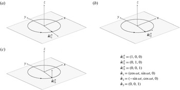
appearing in (4.4)), which, theoretically speaking, corresponds to defining an infinitesimal ‘oriented’ surface around the point source. Without loss of generality, we will account for three limiting cases: (i)
 $\hat{\boldsymbol{n}}|_{1}^{{\it\eta}}=(1,0,0)$
, corresponding to a unit normal vector in the disk plane, well representing a point at the tip of a rotating blade; (ii)
 $\hat{\boldsymbol{n}}|_{2}^{{\it\eta}}=(0,1,0)$
, a vector still located in the rotational plane, but parallel to the rotpole velocity, simulating a point at blade leading edge; (iii)
 $\hat{\boldsymbol{n}}|_{3}^{{\it\eta}}=(0,0,1)$
, that is a vector orthogonal to the disk and corresponding, more or less, to a generic point on the suction side of the blade. A sketch of these vectors is shown in figure 12, with the corresponding
 $O(xyz)$
components to be used in the computation of the
 $k_{L}$
function. By using (4.1b
), (4.7a
), (4.5) and (4.6) it is possible to write down an analytical form for each of the abovementioned parameters and to analyse their behaviour as a function of
 $r$
. Nevertheless, this result can also be achieved by simply reasoning about the orientation of the vector
 $\hat{\boldsymbol{n}}$
and the 2D nature of the rotational motion.
The unit normal vectors
 $\hat{\boldsymbol{n}}$
used to analyse the behaviour of the
 $k_{L}$
function.

As already said, if we assume the rotpole to be a point of a rigid body, the unit normal vector is a time function just by virtue of the rotation; thus, the 2D nature of the rotational motion (
 $v_{z}=0$
) always cancels the corresponding (third) component of
 $\dot{\hat{\boldsymbol{n}}}$
, independently of
 $\hat{\boldsymbol{n}}$
(see (4.6)). This means that, like
 ${\dot{M}}_{i}\hat{r}_{i}$
and
 $M_{r}$
, the term
 $\dot{\hat{n}}_{i}\hat{r}_{i}$
(given by (4.7g
)) does not change with
 $r$
in the disk plane (
 $z_{P}=0$
), while it introduces an additional
 $1/r$
dependence on the kernel function out of the plane of motion (
 $z_{P}\neq 0$
). Concerning
 $\cos {\it\theta}=\hat{n}_{i}\hat{r}_{i}=(\hat{\boldsymbol{n}}\boldsymbol{\cdot }\boldsymbol{r})/r$
, given by (4.7f
), at measurement points located in the plane of rotation (
 $z_{P}=0$
), the scalar product in the numerator always balances the
 $r$
appearing in the denominator; thus, in the disk plane, also
 $\cos {\it\theta}$
does not change with
 $r$
. On the contrary, out of that plane the behaviour depends on
 $\hat{\boldsymbol{n}}$
, and two different cases may occur: (i) if the unit normal vector lies in the disk plane (
 $n_{3}=0$
, as for
 $\hat{\boldsymbol{n}}_{1}$
and
 $\hat{\boldsymbol{n}}_{2}$
), the scalar product cancels the
 $z_{P}$
term in the numerator and
 $\cos {\it\theta}$
introduces a further
 $1/r$
dependence in
 $k_{L}$
; (ii) if the unit normal vector does not lie in the disk plane (
 $n_{3}\neq 0$
, as for
 $\hat{\boldsymbol{n}}_{3}$
), the numerator fully balances the source-observer distance in the denominator and
 $\cos {\it\theta}$
will provide a constant value moving further and further away from the source. For clarity, some examples are explicitly shown in figure 13, where the arrows indicate the increasing order (
 $i=1,2,\ldots \,$
) of measurement points, as listed in table 1. Figure 13(a,b) shows the function
 $\dot{\hat{n}}_{i}\hat{r}_{i}$
as determined at measurement points
 $A_{i}$
located in the plane of motion (a) and at points
 $B_{i}$
out of the disk plane (b), by setting
 $\hat{\boldsymbol{n}}=\hat{\boldsymbol{n}}_{1}$
. The function, of course, oscillates in the revolution period because of the rotation, but in the first case this fluctuation is not altered by the value of the source-observer distance, while in the second case it tends to vanish moving away from the source. Analogously, the function
 $\cos {\it\theta}=\hat{n}_{i}\hat{r}_{i}$
never changes with
 $r$
in the disk plane (as shown in figure 13(c,d), referred to
 $\hat{\boldsymbol{n}}_{1}$
in (c) and
 $\hat{\boldsymbol{n}}_{2}$
in (d)).
Plots of
 $\dot{\hat{n}}_{i}\hat{r}_{i}$
and
 $\cos {\it\theta}$
at points
 $A_{i}$
and
 $B_{i}$
(see table 1), for different
 $\hat{\boldsymbol{n}}$
: (a)
 $\dot{\hat{n}}_{1}\boldsymbol{\cdot }\hat{\boldsymbol{r}}$
at
 $A_{i}$
(disk plane), (b)
 $\dot{\hat{n}}_{1}\boldsymbol{\cdot }\hat{\boldsymbol{r}}$
at
 $B_{i}$
(out of disk plane), (c)
 $\cos {\it\theta}=\hat{n}_{1}\boldsymbol{\cdot }\hat{\boldsymbol{r}}$
at
 $A_{i}$
(disk plane), (d)
 $\cos {\it\theta}=\hat{n}_{2}\boldsymbol{\cdot }\hat{\boldsymbol{r}}$
at
 $A_{i}$
(disk plane), (e)
 $\cos {\it\theta}=\hat{n}_{2}\boldsymbol{\cdot }\hat{\boldsymbol{r}}$
at
 $B_{i}$
(out of disk plane), (f)
 $\cos {\it\theta}=\hat{n}_{3}\boldsymbol{\cdot }\hat{\boldsymbol{r}}$
at
 $B_{i}$
(out of disk plane).

On the contrary, out of the plane of motion the same function exhibits a
 $1/r$
dependence when the unit normal vector has a
 $z$
-component equal to zero (as for
 $\hat{\boldsymbol{n}}_{2}$
, figure 13
e) or, alternatively, it does not change with
 $r$
when this component is not zero (as for
 $\hat{\boldsymbol{n}}_{3}$
, figure 13
f). Here, in particular,
 $\hat{\boldsymbol{n}}_{3}$
is just orthogonal to the disk plane, as the measurement line
 $B$
; then, the function ‘feels’ the rotation in the proximity of the source, but at the furthest points
 $B_{i}$
it tends to assume the value 1, since the vectors
 $\hat{\boldsymbol{n}}$
and
 $\hat{\boldsymbol{r}}$
tend to be parallel (
 ${\it\theta}$
tends to zero).
Rotpole loading kernel function decay in the disk plane (line
 $A$
) at
 $M_{R}=0.8$
for
 $\hat{\boldsymbol{n}}_{1}$
(a) and
 $\hat{\boldsymbol{n}}_{2}$
(b).

Coming back to the loading kernel function, it is quite clear now that (4.3) represents the
 $k_{L}$
function just at points located in the plane of rotation, where the loading term actually exhibits a far-field component depending on
 $1/r$
and a near-field one following the
 $1/r^{2}$
decay law. Figure 14 depicts the numerical solutions of this equation along the measurement line
 $A$
(disk plane), for
 $\hat{\boldsymbol{n}}=\hat{\boldsymbol{n}}_{1}$
(a) and
 $\hat{\boldsymbol{n}}=\hat{\boldsymbol{n}}_{2}$
(b) at
 $M_{R}=0.8$
. At such a high value of the rotational speed, the contribution from the near-field component seems to be non-negligible only for
 $\hat{\boldsymbol{n}}=\hat{\boldsymbol{n}}_{2}$
and very close to the source: in general, the whole acoustic field is dominated by the far-field term and the overall SPL soon aligns to the inverse law
 $1/r$
. This behaviour is very similar to the function
 $k_{T}$
shown in figure 7(a), and the notable gap in the corresponding SPL values confirms that, in the plane of motion and at this blade rate, the thickness noise component can be dominant, depending, of course, on the actual operating conditions and the role played by the ‘unsteady’ source strength
 $\dot{\tilde{p}}$
.
Rotpole loading kernel function decay in the disk plane (line
 $A$
) at
 $M_{R}=0.01$
for
 $\hat{\boldsymbol{n}}_{1}$
(a) and
 $\hat{\boldsymbol{n}}_{2}$
(b).

In any case, by reducing the rotational speed to a realistic value for marine devices (
 $M_{R}=0.01$
, figure 15), the general trend of the SPL decay curve changes again: the near-field term becomes dominant for an extended region and gives rise to a much more relevant drop of the overall noise level. It is worth noting that, for both
 $\hat{\boldsymbol{n}}_{1}$
and
 $\hat{\boldsymbol{n}}_{2}$
, a full realignment with the
 $1/r$
law is reached just at point
 $A_{9}$
, at half a kilometre from the rotpole, and that for
 $\hat{\boldsymbol{n}}=\hat{\boldsymbol{n}}_{3}$
the
 $k_{L}$
function (in the disk plane) is zero. As for
 $k_{T}$
, moving out of the plane of motion, the behaviour of
 $k_{L}$
becomes more intriguing. Whether or not the normal vector
 $\hat{\boldsymbol{n}}$
lies in the disk plane, both
 $\cos {\it\theta}$
and
 $\dot{\hat{n}}_{i}\hat{r}_{i}$
(as well as
 ${\dot{M}}_{i}\hat{r}_{i}$
and
 $M_{r}$
) introduce an additional
 $1/r$
dependence in the integral kernels on the loading component; then, (4.3) should be (more correctly) written in the following form:
 $$\begin{eqnarray}\displaystyle k_{L}({\it\omega},r,c_{0},\hat{\boldsymbol{n}}) & = & \displaystyle \left\{\frac{1}{r^{2}}\left[\frac{\hat{n}_{i}r_{i}}{c_{0}|1-M_{r}|^{2}}+\frac{\dot{\hat{n}}_{i}r_{i}-c_{0}M_{n}}{c_{0}|1-M_{r}|^{2}}\right]\right\}^{F}\nonumber\\ \displaystyle & & \displaystyle +\,\left\{\frac{1}{r^{3}}\left[\frac{\hat{n}_{i}r_{i}}{|1-M_{r}|^{2}}+\frac{({\dot{M}}_{i}r_{i})\hat{n}_{i}r_{i}}{c_{0}|1-M_{r}|^{3}}-\frac{\hat{n}_{i}r_{i}M^{2}}{|1-M_{r}|^{3}}\right]\right\}^{N}\nonumber\\ \displaystyle & & \displaystyle +\,\left\{\frac{1}{r^{4}}\left[\frac{\hat{n}_{i}r_{i}(M_{i}r_{i})}{|1-M_{r}|^{3}}\right]\right\}^{VN}.\end{eqnarray}$$
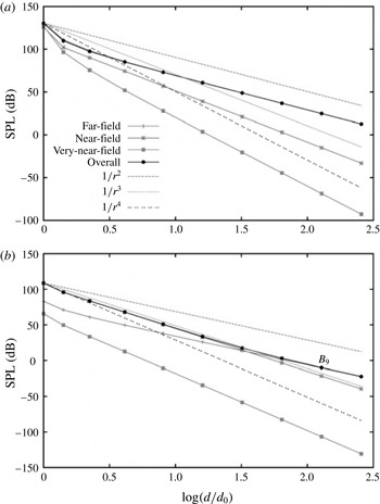
Equation (4.10) states that, moving far from the source and out of the disk plane, the loading noise can propagate along three separate components, which follow the
 $1/r^{2}$
(far-field),
 $1/r^{3}$
(near-field) and
 $1/r^{4}$
(very-near-field) decay laws. These components are shown in figure 16, where, for brevity, only the normal vectors
 $\hat{\boldsymbol{n}}_{1}$
at
 $M_{R}=0.8$
(a) and
 $\hat{\boldsymbol{n}}_{2}$
at
 $M_{R}=0.01$
(b) are shown. The curves show the perfect alignment of the different terms with the abovementioned reference laws, the negligible contribution always provided by the very-near-field term and still (and above all) that accounting for the lowest rotational speed imposes the near-field component as the dominant one for a large part of the whole acoustic field. In this case, this means a drop of the overall SPL ruled by the very stringent
 $1/r^{3}$
law, so that when the overall SPL finally realigns to the inverse law (more or less at point
 $B_{9}$
, at 256 m from the disk plane), the kernel function is very close to zero.
By accounting for
 $\hat{\boldsymbol{n}}_{3}$
(
 $n_{z}\neq 0$
),
 $\cos {\it\theta}$
does not change moving far from the rotpole; in this case, the
 $k_{L}$
function should be written in the further alternative form
 $$\begin{eqnarray}\displaystyle k_{L}({\it\omega},r,c_{0},\hat{\boldsymbol{n}}) & = & \displaystyle \left\{\frac{1}{r}\left[\frac{\cos {\it\theta}}{c_{0}|1-M_{r}|^{2}}\right]\right\}^{F}\nonumber\\ \displaystyle & & \displaystyle +\,\left\{\frac{1}{r^{2}}\left[\frac{\dot{\hat{n}}_{i}r_{i}+c_{0}\left(\cos {\it\theta}-M_{n}\right)}{c_{0}|1-M_{r}|^{2}}+\frac{({\dot{M}}_{i}r_{i})\cos {\it\theta}}{c_{0}|1-M_{r}|^{3}}-\frac{M^{2}\cos {\it\theta}}{|1-M_{r}|^{3}}\right]\right\}^{N}\nonumber\\ \displaystyle & & \displaystyle +\,\left\{\frac{1}{r^{3}}\left[\frac{\cos {\it\theta}(M_{i}r_{i})}{|1-M_{r}|^{3}}\right]\right\}^{VN},\end{eqnarray}$$
so as to point out the coexistence of three separate components, now following the
 $1/r$
,
 $1/r^{2}$
and
 $1/r^{3}$
decay laws. It should be noted that for
 $\hat{\boldsymbol{n}}=\hat{\boldsymbol{n}}_{3}$
the loading kernel function is zero at the first point
 $B_{1}$
(
 $M_{n}=n_{1}=n_{2}=z_{P}=0$
), and the decay curves start from point
 $B_{2}$
, as depicted in figure 17, showing the SPL of the corresponding
 $k_{L}$
function at
 $M_{R}=0.8$
(a) and
 $M_{R}=0.01$
(a). In this case, the near-field component dominates the whole field, independently of the rotational Mach number, while both the very-near- and far-field terms seem to be completely negligible; however, as already mentioned, the role played by the far-field component could be altered significantly by the unsteadiness of the problem and the kernel characterized by the strength
 $\dot{\tilde{p}}$
. At this stage, regardless of the local orientation of the normal vector and the steady or unsteady nature of the underlying aero/hydrodynamic problem, it is very important to stress the fundamental result achieved by our analysis: in the presence of a rotational motion, the noise propagation mechanisms are ruled by the rotational speed.
Rotpole loading kernel function decay out of the disk plane (line
 $B$
) at
 $M_{R}=0.8$
for
 $\hat{\boldsymbol{n}}_{1}$
(a) and
 $M_{R}=0.01$
for
 $\hat{\boldsymbol{n}}_{2}$
(b).

This result (i) represents an essential feature of a rotating source, (ii) heavily affects its behaviour in the near field and (iii) is hardly recognizable through the theoretical models of monopoles and dipoles. The relationship between the propagation mechanisms and
 ${\it\omega}$
can only be of kinematic nature and due to the source auto-interactions occurring within the revolution. In the usual range of velocities for aeronautical devices, these interactions rapidly damp down: the near field is spatially very limited and the wave fronts generated by the body surface (that is, the thickness and loading noise components) soon stabilize and dominate the far field. On the contrary, in the range of velocities for a marine propeller, the near field becomes much larger and the same interactions increase significantly, giving rise to a more pronounced and rapid drop of noise. Such a behaviour is caused by the dominance of noise components dictated by more stringent decay laws compared with
 $1/r$
, and proves the destructive nature of the abovementioned auto-interactions, as for dipoles and quadrupoles, compared with monopoles. This result suggests the existence of a sharp-cutting borderline between the aeroacoustic and hydroacoustic analysis of rotating blades, especially when (as will be shown in § 5) different blades rotate simultaneously.
Rotpole loading kernel function decay out of the disk plane (line
 $B$
) at
 $M_{R}=0.8$
(a) and
 $M_{R}=0.01$
for
 $\hat{\boldsymbol{n}}_{3}$
(b).

4.4 Kernel function maps
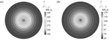
Some additional interesting features of the rotpole kernel functions can be found by computing the maps of the overall SPL and assessing the corresponding directivity in different planes. Figure 18 shows the dB isocurves of the
 $k_{T}$
SPL in the disk plane, at
 $M_{R}=0.8$
(a) and
 $M_{R}=0.01$
(b), determined on a polar mesh of
 $200\times 80$
measurement points, covering an area of
 $100R$
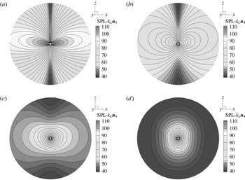
. As expected, in this plane the thickness integral kernel always exhibits a radial directivity and, then, a uniform decay in all directions. Nevertheless, the drop of the SPL is very different in the two cases, following the inverse and the inverse-squared laws at the highest and the lowest rotational speed respectively. This can be easily verified through the different range of values (see the legends of figure 18
a,b) or, alternatively, the comparison between figures 7(a) and 8(b). The radial directivity just arises from the symmetry of the motion in its own plane and represents, de facto, the only affinity between the rotpole thickness term and a monopole source.
Thickness kernel function maps in the
 $xy$
(disk) plane for a rotpole at
 $M_{R}=0.8$
(a) and
 $M_{R}=0.01$
(b).

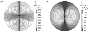
Thickness kernel function maps in the
 $xz$
plane (orthogonal to disk plane) for a rotpole at
 $M_{R}=0.8$
(a) and
 $M_{R}=0.01$
(b).

In fact, by moving out of the disk, the
 $k_{T}$
directivity abruptly changes and exhibits the typical two-lobed structure of a dipole source, as shown in the two
 $xz$
maps of figure 19, still depicted with a different scale because of the notable variation of the SPL range. It can be noted how, at the highest value of the rotational speed, the
 $k_{T}$
SPL isocurves are more pressed towards the disk plane, while at
 $M_{R}=0.01$
the lobes appear to be more circular and uniformly distributed. The SPL maps of the loading kernel function in the disk plane are, in essence, identical to the ones of
 $k_{T}$
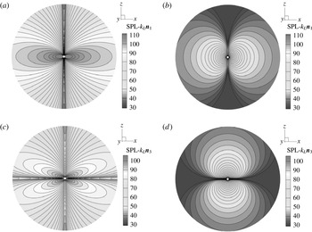
(figure 18) and are not reported. On the contrary, it is interesting to look at the
 $k_{L}$
maps in the
 $xz$
plane, depicted in figure 20, still for
 $M_{R}=0.8$
(a) and
 $M_{R}=0.01$
(b), but referred to a different choice of the unit normal vector, (
 $\hat{\boldsymbol{n}}_{1}$
and
 $\hat{\boldsymbol{n}}_{3}$
in (a,b) and (c,d) respectively). When the unit vector lies in the plane of motion, the
 $k_{L}$
contour map at
 $M_{R}=0.8$
shows the expected two-lobed structure of a dipole, which (as for
 $k_{T}$
) becomes more uniform by decreasing the rotational speed. Nevertheless, for a unit vector orthogonal to the plane of motion, the same function at the highest speed exhibits a typical quadrupolar structure, which turns back into a two-lobed shape at
 $M_{R}=0.01$
with the dipole axis now orthogonal to the disk plane.
Loading kernel function maps in the
 $xz$
(out of disk) plane for a rotpole at
 $M_{R}=0.8$
(a,c) and
 $M_{R}=0.01$
(b,d) for (a,b)
 $\hat{\boldsymbol{n}}_{1}$
and (c,d)
 $\hat{\boldsymbol{n}}_{3}$
.

Looking at these last results, it is evident how both the rotational speed and the normal vector may have a deep influence on the directivity of the loading noise component. For this reason, we accounted for an additional more generic vector
 $\hat{\boldsymbol{n}}=\hat{\boldsymbol{n}}_{4}$
, by using the triad
 $\hat{\boldsymbol{n}}|^{{\it\eta}}=(\sqrt{2}/4,\sqrt{2}/4,\sqrt{3}/2)$
; this choice corresponds to a vector making an angle
 ${\it\beta}=60^{\circ }$
with the
 $xy$
plane and an angle
 ${\it\gamma}=45^{\circ }$
with the local
 ${\it\eta}_{1}$
and
 ${\it\eta}_{2}$
axes, so that in the main reference
 $O(xyz)$
its components become
 $\hat{\boldsymbol{n}}_{4}=(\sqrt{2}/4\cos {\it\omega}t-\sqrt{2}/4\sin {\it\omega}t,\sqrt{2}/4\sin {\it\omega}t+\sqrt{2}/4\cos {\it\omega}t,\sqrt{3}/2)$
. The
 $k_{L}$
SPL maps corresponding to
 $\hat{\boldsymbol{n}}_{4}$
are depicted in figure 21, at four different values of the rotational Mach number and now using the same range for SPL values. The main dipole nature of an aeronautical
 $k_{L}$
out of the disk plane is confirmed by the two lobes occurring at
 $M_{R}=0.8$
(figure 21
a), although the map shows a slight asymmetry along the ‘dominant’ vertical direction of the fixed vector
 $\hat{\boldsymbol{n}}_{4}$
. By decreasing the speed to
 $M_{R}=0.4$
(figure 21
b) this asymmetry becomes more evident, while a further reduction of the Mach number (
 $M_{R}=0.08$
, figure 21
c) progressively reduces the two-lobed shape of the SPL contour map. Finally, at
 $M_{R}=0.01$
, the map confirms the impressive drop of the overall SPL and shows, for a marine
 $k_{L}$
, a structure similar to an elongated monopole source. It is worth pointing out that these maps just refer to the
 $k_{L}$
function of a single rotpole, equipped with an artificially imposed
 $\hat{\boldsymbol{n}}$
, and in a fixed plane; they do not represent the 3D directivity of the loading noise due to a general blade, whose trend is certainly affected by the shape of the body too. Nevertheless, they emphasize very well how the acoustic behaviour of a rotating source strongly depends on the rotational speed, not only in terms of intensity (as previously shown through the noise decay curves), but also in terms of directivity.
Loading kernel function maps in the
 $xz$
plane for a rotpole equipped with
 $\hat{\boldsymbol{n}}=\hat{\boldsymbol{n}}_{4}$
, at
 $M_{R}=0.8$
(a),
 $M_{R}=0.4$
(b),
 $M_{R}=0.04$
(c) and
 $M_{R}=0.01$
(d).

5 Multiple rotpoles
The analysis of the kernel functions for a single rotpole has shown how the SPL decay notably increases at a low (marine) rotational speed, and that this decay is dictated by the mutual interactions of the disturbances generated by the source along its own circular trajectory. For this reason, rather than a generic interaction, we should talk of a destructive interference. Then, a very interesting question arises: what would happen if such an interference were directly imposed by the presence of one (or more) additional rotpole(s)? As is well known, the elemental dipole and quadrupole sources can be represented through a suitable combination of monopoles, and their lower acoustic efficiency is just caused by the mutual interaction of the single elements. The situation, in this case, is very similar, and a definite answer to the above question can be achieved by accounting for rotpoles of
 $n$
th order, where
 $n$
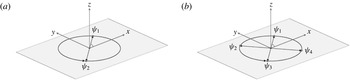
(spatially shifted) sources rotate simultaneously. In particular, just like dipoles and quadrupoles, we will assess here the behaviour of a dirotpole and a quadrurotpole, constituted by two and four rotpoles with the same direction of rotation (analogously to what happens in a multibladed propeller), shifted by
 ${\it\beta}_{d}=j{\rm\pi}$
(with
 $j=0,1$
) and
 ${\it\beta}_{q}=j{\rm\pi}/2$
(with
 $j=0,1,2,3$
) respectively. A sketch of these multiple rotating sources is shown in figure 22, where
 ${\it\psi}_{j}={\it\omega}t+{\it\beta}_{j}$
indicates the azimuth angle of the
 $j\text{th}$
rotpole.
The dirotpole (a) and the quadrurotpole (b) sources.

From a numerical point of view, the behaviour of a rotpole of
 $n$
th order can still be examined through the kernel functions, by adding up the contributions from the single sources; then, (4.2) and (4.3) are replaced by
 $$\begin{eqnarray}\left\{k_{T}\right\}^{n}({\it\omega},r_{j},c_{0})=\mathop{\sum }_{j=1}^{n}\left\{\frac{1}{r}\left[\frac{{\dot{M}}_{i}\hat{r}_{i}}{|1-M_{r}|^{3}}\right]\right\}_{j}^{F}+\left\{\frac{1}{r^{2}}\left[\frac{c_{0}\left(M_{r}-M^{2}\right)}{|1-M_{r}|^{3}}\right]\right\}_{j}^{N},\end{eqnarray}$$
 $$\begin{eqnarray}\displaystyle \left\{k_{L}\right\}^{n}({\it\omega},r_{j},c_{0},\hat{\boldsymbol{n}}_{j}) & = & \displaystyle \mathop{\sum }_{j=1}^{n}\left\{\frac{1}{r}\left[\frac{\cos {\it\theta}}{c_{0}|1-M_{r}|^{2}}+\frac{\dot{\hat{n}}_{i}\hat{r}_{i}}{c_{0}|1-M_{r}|^{2}}+\frac{{\dot{M}}_{i}\hat{r}_{i}\cos {\it\theta}}{c_{0}|1-M_{r}|^{3}}\right]\right\}_{j}^{F}\nonumber\\ \displaystyle & & \displaystyle +\,\left\{\frac{1}{r^{2}}\left[\frac{\cos {\it\theta}-M_{n}}{|1-M_{r}|^{2}}+\frac{c_{0}\left(M_{r}-M^{2}\right)}{|1-M_{r}|^{3}}\right]\right\}_{j}^{N},\end{eqnarray}$$
where the coordinates of
 $j$
th rotpole, of course, are
 $$\begin{eqnarray}\mathscr{R}_{j}\equiv \{R\cos ({\it\omega}t+{\it\beta}_{j}),R\sin ({\it\omega}t+{\it\beta}_{j}),0\}\end{eqnarray}$$
and (4.7) has to be changed accordingly. It is worth pointing out that, concerning
 $\{k_{L}\}^{n}$
, the single elements of the multiple source are associated with a unique choice for
 $\hat{\boldsymbol{n}}$
, and, in the following, the SPL of the kernel functions will be determined by explicitly removing the possible mean value in (5.1), (5.2), so as to point out the effects of the abovementioned destructive interference on the pure fluctuating ‘tonal’ component of the integral terms (which, acoustically speaking, is the only relevant one).
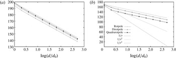
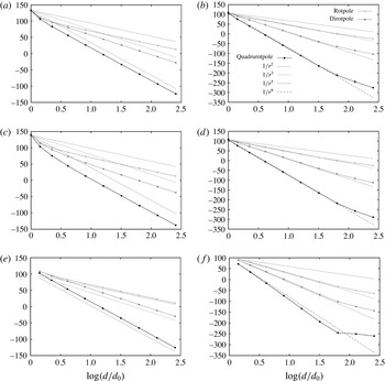
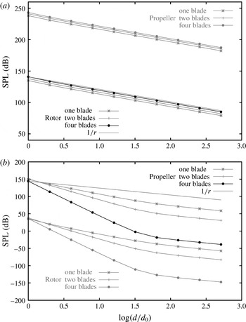
Let us start the analysis by taking into account the typical Mach numbers of an aeronautical device and the thickness kernel function. Figure 23 shows the comparison between the
 $\{k_{T}\}^{n}$
noise decay curves, determined by (5.1) along measurement line
 $A$
(disk plane), for a single rotpole (
 $n=1$
), a dirotpole (
 $n=2$
) and a quadrurotpole (
 $n=4$
), at
 $M_{R}=0.8$
(a) and
 $M_{R}=0.4$
(b). At the highest value of the velocity, no particular interaction occurs between the single sources: as expected, all the curves soon align to the inverse law
 $1/r$
, and the presence of additional sources actually gives rise to a slight increase of the overall SPL. At
 $M_{R}=0.4$
, however, the general trend changes. The rotpole and dirotpole curves, in fact, now perfectly overlap, while the noise decay of the quadrurotpole becomes more pronounced in the proximity of the source (between
 $A_{1}$
and
 $A_{2}$
), where the curve aligns to the
 $1/r^{3}$
reference law. Then, although the realignment with the
 $1/r$
line occurs fairly quickly, at a few metres from the origin, the lower speed triggers a destructive interference between the single rotpoles.
The
 $\{k_{T}\}^{n}$
function decay for a rotpole, dirotpole and quadrurotpole in the disk plane (line
 $A$
), at
 $M_{R}=0.8$
(a) and
 $M_{R}=0.4$
(b).

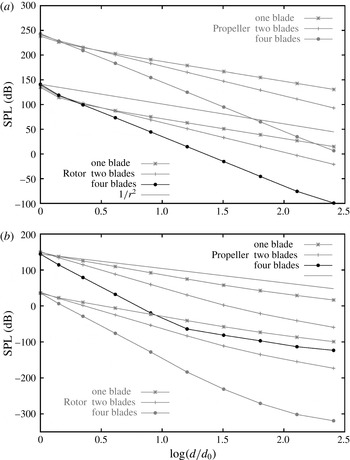
The
 $\{k_{T}\}^{n}$
function decay for a rotpole, dirotpole and quadrurotpole in the disk plane (line
 $A$
), at
 $M_{R}=0.08$
(a) and
 $M_{R}=0.01$
(b).

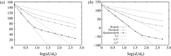
By reducing the rotational Mach number, this interference increases significantly. At
 $M_{R}=0.08$
(figure 24
a), the SPL decay of the dirotpole exhibits a starting slope aligned to
 $1/r^{3}$
, and when the curve assumes the trend of the inverse law (more or less at point
 $A_{5}$
), the SPL has already fallen down to
 $95$
dB and exhibits a gap of more than
 $30$
dB with respect to the
 $1/r$
line. The drop suffered by the quadrurotpole
 $k_{T}$
function is much more pronounced: up to
 $8~\text{m}$
from the origin (point
 $A_{3}$
), the slope of the curve even follows the
 $1/r^{5}$
law, corresponding to a decrease of
 $30$
dB at each doubling of distance, so that when the curve regains the trend of the inverse law (still at point
 $A_{5}$
), the SPL value has fallen down to
 $55$
dB. At a more realistic rotational speed for a marine propeller (
 $M_{R}=0.01$
), the drop of the overall SPL for multirotpoles becomes impressive, as shown in figure 24(b). In this case, the alignment of the decay curves of the dirotpole and the quadrurotpole with the
 $1/r^{3}$
and
 $1/r^{5}$
laws respectively extends for a large part of the field, up to point
 $A_{6}$
, located at 64 m from the origin. This means that, at such a value of the rotational Mach number, the thickness term along line
 $A$
(disk plane) simply collapses in a spatially very limited region, and its contribution to the acoustic field is destined to vanish very rapidly.
Numerical solution of (5.1) at point
 $A_{4}$
, for a quadrurotpole, a dirotpole and the single rotpoles at
 $M_{R}=0.8$
(a) and
 $M_{R}=0.01$
(b).

Such a shocking drop of the overall SPL from multirotpoles can be easily explained by looking at the corresponding time histories of the
 $\{k_{T}\}^{n}$
function. Figure 25 shows the numerical solution of (5.1) at the disk plane point
 $A_{4}$
(
 $16~\text{m}$
from the origin) for the dirotpole, the quadrurotpole and each of the single rotpoles, at
 $M_{R}=0.8$
(a) and
 $M_{R}=0.01$
(b). At the highest speed, the kernel functions from the separate sources show a fluctuating waveform affecting, more or less, a quarter of a period; thus, by adding the contributions from the single rotpoles, no relevant interaction occurs and the solutions for the multirotpoles are characterized by two or four peak values very similar to the ones from the single elements. On the contrary, by bringing down
 ${\it\omega}$
, the fluctuation not only reduces in amplitude, but progressively covers a larger part of the revolution period; therefore, by adding the contributions from the single sources, a destructive interference between the time-shifted
 $k_{T}$
functions results.
The
 $\{k_{T}\}^{n}$
function decay for a rotpole, dirotpole and quadrurotpole out of the disk plane (line
 $B$
), at
 $M_{R}=0.8$
(a) and
 $M_{R}=0.01$
(b).

This result is shown in figure 25(b), referred to
 $M_{R}=0.01$
: besides the notable variation of the range values, the multirotpoles give rise to a mutual cancellation of the single components, and at only
 $16~\text{m}$
from the rotation axis (point
 $A_{4}$
), the dirotpole
 $\{k_{T}\}^{2}$
function provides a much lower (approximately
 $80\,\%$
less) peak value compared with the single source, while the
 $\{k_{T}\}^{4}$
function of the quadrurotpole is very close to zero. Out of the plane of motion, the destructive interference occurs also at the higher rotational velocities. In this case, in fact, the
 $k_{T}$
function decreases much more rapidly than in the disk plane (see figure 10
a), and the time histories from each source soon interact with each other, in a way very similar to that shown in figure 25(b). Figure 26 shows the decay curves along line
 $B$
, out of the disk plane. At
 $M_{R}=0.8$
(a), the SPL for
 $\{k_{T}\}^{n}$
follows the
 $1/r^{2}$
,
 $1/r^{3}$
and even the
 $1/r^{5}$
reference laws for the rotpole, the dirotpole and the quadrurotpole respectively; this result confirms (and, somehow, better explains) the lower noise level provided by multibladed propellers and rotors in both marine and aeronautical applications. At
 $M_{R}=0.01$
(b), however, the SPL drop becomes really devastating. At such a low value of the rotational speed, as already shown in figure 11(b), the
 $k_{T}$
function (expressed by (4.9)) aligns to the stringent
 $1/r^{3}$
law for an extended region. Nevertheless, in the presence of multiple sources, the interferences occurring in the near field (up to point
 $B_{7}$
) increase and the dirotpole
 $\{k_{T}\}^{2}$
function follows the
 $1/r^{5}$
decay law, while the quadrurotpole function even aligns to the
 $1/r^{9}$
reference line, thus approaching zero at point
 $B_{4}$
, at only
 $8~\text{m}$
from the origin. In other words, at
 $M_{R}=0.01$
and out of the disk plane, the thickness kernel function for a quadrurotpole vanishes in a handful of radii from the rotation axis. The behaviour of the loading kernel function
 $\{k_{L}\}^{n}$
, provided by (5.2) for multirotpoles, is very similar to
 $\{k_{T}\}^{n}$
; here, for brevity, it is reported only at the highest and lowest values of the tested rotational velocities. Figure 27 shows the SPL decay curves along line
 $A$
(disk plane) for multiple sources rotating at
 $M_{R}=0.8$
(a,c) and
 $M_{R}=0.01$
(b,d), corresponding to
 $\hat{\boldsymbol{n}}=\hat{\boldsymbol{n}}_{1}$
(a,b) and
 $\hat{\boldsymbol{n}}=\hat{\boldsymbol{n}}_{2}$
(c,d). As for the thickness term, at the high speed and in the plane of motion, the presence of simultaneously rotating sources slightly increases the overall noise level, and the decay curves soon align to the typical far-field inverse law
 $1/r$
. On the other
The
 $\{k_{L}\}^{n}$
function decay for a rotpole, dirotpole and quadrurotpole in the disk plane (line
 $A$
), at
 $M_{R}=0.8$
(a,c) and
 $M_{R}=0.01$
(b,d) for
 $\hat{\boldsymbol{n}}=\hat{\boldsymbol{n}}_{1}$
(a,b) and
 $\hat{\boldsymbol{n}}=\hat{\boldsymbol{n}}_{2}$
(c,d).

hand, as the speed is reduced, the destructive interference occurs and rapidly increases. As said above, for a single rotpole at
 $M_{R}=0.01$
the phenomenon is necessarily auto-induced by the rotational motion, and in a large region (the near field) it causes a drop of the SPL ruled by the inverse-squared law. The presence of additional sources makes the interference more intense and gives rise, in the same region, to a trend of the overall SPL now ruled by the
 $1/r^{3}$
and
 $1/r^{5}$
laws for the dirotpole and the quadrurotpole respectively. The behaviour of the
 $\{k_{L}\}^{n}$
function out of the plane of motion is even more impressive and is shown in figure 28 for
 $M_{R}=0.8$
(a,c,e) and
 $M_{R}=0.01$
(b,d,f), now also showing the case
 $\hat{\boldsymbol{n}}=\hat{\boldsymbol{n}}_{3}$
(e,f). These results demonstrate the deep influence of the rotational speed on the integral kernels of the loading source term, along the measurement line
 $B$
: in a region of approximately
 $128$
radii from the rotation axis (up to point
 $B_{8}$
) and turning
 $M_{R}$
from
 $0.8$
to
 $0.01$
, the
 $\{k_{L}\}^{n}$
SPL turns from a trend ruled by the
 $1/r^{2}$
law to
 $1/r^{3}$
for the single rotpole, from
 $1/r^{3}$
to
 $1/r^{5}$
for the dirotpole and even from
 $1/r^{5}$
to
 $1/r^{9}$
for the quadrurotpole. It is interesting to note how this behaviour is totally independent of the normal vector: as depicted in figure 25, in fact, the destructive interference arises from the time shift of pressure disturbances spread over the whole revolution period, which is a mechanism not related at all to the selected orientation of
 $\hat{\boldsymbol{n}}$
. On the contrary, this mechanism could be notably affected by the unsteadiness of the underlying aero/hydrodynamic solution, which implicitly entails different contributions from the single sources and reckons the unknown balance between the
 $\{k_{L}\}^{n}$
(far-field) components characterized by
 $\tilde{p}$
and
 $\dot{\tilde{p}}$
. This issue will be briefly discussed in § 7; nevertheless, all of these results confirm the strict dependence of noise propagation on
 ${\it\omega}$
, and, above all, the occurrence of an impressive destructive interference in the case of multiple sources at low rotational speed.
The
 $\{k_{L}\}^{n}$
function decay for a rotpole, dirotpole and quadrurotpole in the disk plane (line
 $A$
), at
 $M_{R}=0.8$
, (a,c,e) and
 $M_{R}=0.01$
(b,d,f) for
 $\hat{\boldsymbol{n}}=\hat{\boldsymbol{n}}_{1}$
(a,b),
 $\hat{\boldsymbol{n}}=\hat{\boldsymbol{n}}_{2}$
(c,d) and
 $\hat{\boldsymbol{n}}=\hat{\boldsymbol{n}}_{3}$
(e,f).

6 Marine propeller ‘versus’ helicopter rotor
The validity of the analysis on the kernel functions for a rotating point source, its relationship with the ‘full’ numerical solution of formulation 1A for a three-dimensional body and, above all, its practical consequences can be demonstrated by performing a very simple standard FWH-based prediction of the thickness noise only, thus avoiding any problem related to the availability of aero/hydrodynamic data. To this end, we will solve (2.2) for both a helicopter rotor and a marine propeller model, here suitably scaled in order to have the same radius
 $R=1~\text{m}$
, at the same operating conditions in air and underwater. Such a test, of course, is just explanatory and also concerns some unrealistic configurations; nevertheless, it enables appreciation of if and how the accounting for different fluids (each with its own values of
 ${\it\rho}_{0}$
and
 $c_{0}$
) and the geometrical differences of the two devices may affect the numerical solution of (2.2). A sketch of the models is shown in figure 29. The marine propeller is the INSEAN E779A, rotating around the
 $x$
axis. As is usual for this kind of device, the blade exhibits a remarkable variation of chord and twist angle along the span and a rather high solidity, with a thickness decreasing from the 60/70 % of the blade towards the tip. On the other hand, the rotor model corresponds to the BO-105 main rotor and rotates around the
 $z$
axis. In this case, both the chord and the thickness spanwise distribution are uniform, and the blade planform has a much higher aspect ratio. We assume that the fluid is at rest and both of the models are simply rotating at a fixed
 $M_{R}$
. The measurement points are located along the measurement lines
 $A$
and
 $B$
of figure 6, here suitably oriented to account for the different rotation axes of the two devices. The rotational velocity
 ${\it\omega}=c_{0}M_{R}/R$
is set according to the speed of sound, being
 $c_{0}=340~\text{m}~\text{s}^{-1}$
for the rotor and
 $c_{0}=1500~\text{m}~\text{s}^{-1}$
for the propeller; furthermore, the fluid density
 ${\it\rho}_{0}$
and the reference pressure for the dB computation are set to
 $1.234~\text{kg}~\text{m}^{-3}$
and
 $1000~\text{kg}~\text{m}^{-3}$
,
 $p_{ref}=2\times 10^{-5}$
Pa and
 $p_{ref}=10^{-6}$
Pa for air and water respectively. The calculations will concern both the single blade of each device and the alternative two-bladed and four-bladed configurations, in order to check the reliability of the results found for the dirotpole and quadrurotpole sources.
Three-dimensional sketches of the E779A marine propeller (a) and the BO-105 helicopter main rotor (b) models, used for thickness noise prediction.

Figure 30 shows the thickness noise decay in the disk plane (line
 $A$
), at
 $M_{R}=0.8$
(a) and
 $M_{R}=0.01$
(b). For clarity, each panel shows the ‘unrealistic’ cases (the marine propeller operating underwater at
 $M_{R}=0.8$
and the rotor in air at
 $M_{R}=0.01$
) in a grey colour. In practice, the decay of thickness noise from the helicopter rotor at
 $M_{R}=0.8$
(figure 30
a) overlaps the inverse law
 $1/r$
, thus confirming the well-known aeroacoustic behaviour of this term in the far field. Moreover, at such a high value of the rotational speed, no destructive interference characterizes the multibladed devices, and the thickness noise from the two- or four-bladed rotors is slightly higher compared with the single blade. The marine propeller exhibits a much higher value of the SPL, due to the very large solidity with respect to the aeronautical blade (
 $R$
being the same), and, above all, the same trend for all of the noise decay curves. This result is very interesting. It confirms that a helicopter rotor in air and a marine propeller in water basically behave in the same way: the surrounding fluid and the shape of the body source determine the overall noise level, but they do not affect the noise propagation mechanisms, which, in essence, are governed by the rotational Mach number.
Thickness noise decay of the E779A propeller and the BO-105 rotor models in the disk plane (line
 $A$
), at
 $M_{R}=0.8$
(a) and
 $M_{R}=0.01$
(b).

The acoustic equivalence of the two devices and the notable reduction of the thickness noise due to the much lower blade rate are confirmed in figure 30(b). As revealed in advance by the kernel function
 $k_{T}$
, the thickness noise from any blade rotating at
 $M_{R}=0.01$
decreases more rapidly in the field, following the
 $1/r^{2}$
law instead of the
 $1/r$
law in a very extended region (see also figures 7 and 8). Furthermore, the mutual interactions characterizing the behaviour of multiple rotating sources make this drop impressive for any multibladed device. The thickness noise decay curves along line
 $B$
, at points located downstream the blades, are shown in figure 31, and fully confirm the intrinsic acoustic features of a rotating source/body examined through the kernel functions. In this case also, in fact, the decay of the thickness term from the rotor in air soon aligns to the inverse-squared law, while the corresponding curve from the propeller underwater, at the lowest speed, shows a deeper slope (
 $1/r^{3}$
) in an extended region and gives rise to a more significant and rapid decrease of the thickness contribution.
Thickness noise decay of the E779A and the BO-105 models out of the disk plane (downstream line
 $B$
), at
 $M_{R}=0.8$
(a) and
 $M_{R}=0.01$
(b).

It can be noted how the curve for the four-bladed rotor at
 $M_{R}=0.8$
(figure 31
a) exhibits a very slight slope change at the last point, while the one from the two-bladed device seems not to change at all. This suggests that the absence of the expected realignment to the inverse-squared law falls down out of the range of distances taken into account here, and, in the presence of multiple sources, the interference mechanisms may affect a spatially very extended region, also at a high rotational rate. In any case, these results perfectly match the decay curves depicted in figures 10(a) and 11(b), referred to a single point source and without any term related to the source strength. Table 2 lists the overall SPLs for the four-bladed propeller at
 $M_{R}=0.01$
(with the distance from the plane of motion) at the first five points along line
 $B$
; these values correspond to the decay curve depicted in figure 31(b). At the disk plane point
 $B_{1}$
the thickness noise level is rather high (
 $144$
dB), but at only
 $8~\text{m}$
from the disk plane (point
 $B_{4}$
) it collapses to 32 dB, and goes to zero before
 $B_{5}$
.
Thickness noise SPLs from the E779A propeller along
 $B$
, at
 $M_{R}=0.01$
.

7 Discussion
At this stage, and in the light of the numerical simulations presented, for example, in Ianniello et al. (Reference Ianniello, Muscari and Di Mascio2013, Reference Ianniello, Muscari and Di Mascio2014a
) or Ianniello & De Bernardis (Reference Ianniello and De Bernardis2015), it could be useful to summarize and briefly discuss the results achieved hitherto. The analysis performed on rotpole kernel functions may be interpreted both as a study of the acoustic behaviour of a rotating point source and, alternatively, as a simple investigation on the general trend of the corresponding surface integral kernels. In both cases, however, it is clear that the way in which the noise propagates in the field is totally ruled by the rotational speed and may give rise to different components, characterized by a
 $1/r$
,
 $1/r^{2}$
,
 $1/r^{3}$
or even a
 $1/r^{4}$
dependence on the source-observer distance. This behaviour has no strict relationship with monopole or dipole models. Thus, even though the surface terms from rotating bodies can always be thought of as generated by a suitable distribution of the elemental sources, the use of the more suitable (although trivial) model of the rotpole provides a much more intuitive and effective representation of the problem. On the other hand, the rotpole (like the dipole and quadrupole) could be thought of as a suitable combination of monopoles.
A schematic representation of the models corresponding to the elemental sources.

As discussed in § 3, a dipole can be represented by a sphere of radius
 $a$
oscillating along a prescribed axis in a very small distance
 $d$
(such that both
 $ka$
and
 $kd$
are
 $\ll 1$
,
 $k=2{\rm\pi}/{\it\lambda}$
being the wavenumber), while a quadrupole is constituted by two close dipoles, with the axes lying or not on the same line, thus giving rise to the longitudinal and lateral quadrupole respectively. These schemes are shown in figure 32. The same figure (c) shows that, by decomposing the circular motion into its harmonic components, the rotpole is nothing but a sort of special quadrupole source, constituted by two orthogonally placed dipoles, where, however, the distance
 $d=2R$
is no longer negligible and assumes the role of a characteristic length of the model. In this way, the actual ‘size’ of the source is not so much related to the radius
 $a$
of the oscillating sphere as to the diameter of the circular trajectory. Undoubtedly, some analytic expression for the pressure radiated by a rotpole can be found, in particular as a function of
 $k$
,
 ${\it\omega}$
and
 $R$
. This topic, however, is beyond the aims of the paper and our practical approach, based on the analysis of the surface integral kernels. In any case, this scheme shows quite clearly how the acoustic nature of a rotating point is more similar to some source of higher order, rather than monopoles and dipoles, which (as is well known) may be characterized by a much lower acoustic efficiency compared with the classic elemental sources. It is also very interesting to note how Farassat originally pointed out the true nature of the thickness surface term, by identifying it through a distribution of dipoles and quadrupoles (Farassat Reference Farassat1974, p. 389).
Any numerical assessment of the surface terms requires the use of a mesh. If a zeroth-order formulation (as usual) is adopted, the integrals are determined by adding up the (constant) kernels at the panel centroids, that is exactly by accounting for a three-dimensional distribution of rotpoles, each equipped with its own source strength, related to the body shape (
 ${\it\rho}_{0}v_{n}$
for thickness) and loads (
 $\tilde{p}$
and
 $\dot{\tilde{p}}$
for loading). This equivalence is well represented in figure 33, showing the blade of a marine propeller and a sketch of the corresponding numerical model. In this way, the FWH equation still depicts the acoustic field from rotating bodies as the sum of surface and volume source terms, but the identification of the surface terms with rotpoles (instead of monopoles and dipoles) suggests a new way to think of the role played by the different components.
The discretized model of a blade surface exactly corresponds to a 3D distribution of rotpoles on the computational mesh (zeroth-order formulation).

In particular, in light of what has been discussed so far, the rather popular belief that at a low subsonic rotational speed the surface terms are dominant seems to be rather questionable and should require, at least, a more accurate explanation of what is meant by ‘high’ or ‘low’ speed. There is no doubt, in fact, that in the usual range of rotational Mach numbers for aeronautical devices (up to the transonic regime and the occurrence of shock waves), the thickness and loading integrals represent the most relevant components of the acoustic field. This certainty comes from decades of experimental and numerical research in aeroacoustics, and, in essence, it is also confirmed by the general trend of rotpole kernel functions at
 $M_{R}=0.8$
and
 $M_{R}=0.4$
. Nonetheless, the same analysis reveals the very poor acoustic efficiency of rotpoles at (marine) low rotational Mach numbers: the lower the speed, the more pronounced (and persisting, in the much larger near field) the decay of the formulation 1A surface terms. Thus, from a hydroacoustic point of view, the above sentence sounds completely wrong: underwater, the thickness and loading components may be relevant just in the proximity of the body and at a very high rotational speed, while at the usual operating condition of a marine propeller, their contribution rapidly falls down and could become completely negligible. The explanation of this behaviour has been provided in different ways. From a mathematical point of view, the relevant drop of the FWH surface terms is explained by the dominance (in an extended region) of integral kernels characterized by a higher-order dependence on
 $r$
, compared with the inverse and inverse-squared laws. From a physical point of view, it is due to the intrinsic kinematic features of the rotational motion and the much more significant destructive interference occurring at low speed between the (pressure) disturbances generated by the source along its own circular trajectory. In a similar (but much more incisive) way to the elemental sources, this interference may become devastating in the case of multiple rotpoles, whose model depicts the behaviour of multibladed devices very well. Most marine propellers have more than three or four blades, for which the drop of the linear kernel functions was shown to reach the impressive
 $1/r^{9}$
law, corresponding to a gap of
 $54$
dB at any doubling of the source-observer distance. In these conditions, the contribution from the surface integrals to the hydroacoustic field would simply vanish at a few radii from the rotating body.
At a first glance, the proposed analysis of the kernel functions seems to leave a substantial margin of uncertainty about the actual role played by an unsteady loading noise component. This uncertainty concerns both the behaviour of the single rotpole (where the different scaling of the integral terms characterized by the source strength
 $\tilde{p}$
and
 $\dot{\tilde{p}}$
could make the
 $1/r$
far-field component more relevant) and that from multiple sources (for which, theoretically speaking, the superimposition of signals with different waveforms is destined to reduce the destructive nature of the mutual interference). On the other hand, the remarkable gap between the near- and far-field contributions shown in figure 17 and the occurrence of very stringent decay laws for both
 $\{k_{T}\}^{n}$
and
 $\{k_{L}\}^{n}$
at
 $M_{R}=0.01$
(
 $1/r^{5}$
for the dirotpole and
 $1/r^{9}$
for the quadrurotpole) suggest that not even a high unsteadiness of the underlying aero/hydrodynamic problem could balance the rapid decay of the surface integrals imposed by the low speed, in the strict proximity of the source. In any case, the abovementioned uncertainty does not affect the main result of the paper, which is the strict relationship between the noise propagation and the rotational rate, and, above all, the inadequacy of any ‘pure linear’ analysis for hydroacoustic purposes. Not by chance, even admitting the aggressiveness of the assumption
 $\tilde{p}=\dot{\tilde{p}}=1$
and a possible overestimation of the decay laws determined for the elemental multirotpole models, all results published in Ianniello et al. (Reference Ianniello, Muscari and Di Mascio2014a
) (concerning the noise prediction from a ship-scaled model) show a rapid annihilation of both thickness and loading terms generated by the installed four-bladed propeller, in spite of the high unsteadiness of the tested operating conditions. In other words, whatever the type of hydrodynamic problem, the FWH surface terms from a multibladed propeller must reckon with the remarkable drop imposed by the very low
 $M_{R}$
, which represents an intrinsic feature of the corresponding integral kernels.
As already said in the introduction, the underwater flow around a propeller is characterized by significant nonlinear phenomena, occurring rather far from the body itself (Felli et al.
Reference Felli, Camussi and Di Felice2011). The photographs shown in figure 34, for example, show this flow downstream of a three-bladed device in open water, at two different values of the advance coefficient
 $J=V/nD$
(where
 $V$
is the inflow velocity,
 $n$
is the rotational speed, usually expressed in rounds per second, and
 $D$
is the propeller diameter). The flow is characterized by an axial swirling wake released from the hub and a vortical wake generated at the blade tip, which persist in an extended region, here approximately equal to
 $10R$
. At
 $J=0.65$
(figure 34
a), both the vortical systems develop downstream in a very regular way and start to destabilize quite far from the body; on the contrary, at
 $J=0.45$
(figure 34
b), corresponding to a higher hydrodynamic load condition for the propeller, the hub wake starts to oscillate at approximately
 $5R$
from the disk, while the blade tip vortex breaks and gives rise to a highly turbulent flow.
The vortical wake and flow instabilities characterizing the underwater flow downstream of a three-bladed propeller in open water conditions, at
 $J=0.65$
(a) and
 $J=0.45$
(b).

Both of the wakes are significant sources of noise, and the flow instabilities (corresponding to higher-velocity gradients in the flow field) locally increase the overall noise level. In the FWH equation, these nonlinear effects are taken into account through the Lighthill tensor and the quadrupole source terms. Theoretically speaking, the noise decay corresponding to a quadrupole source should follow the
 $1/r^{4}$
law, a value perfectly comparable with (and, in some cases, much less stringent than) the analysed drop of the surface terms. If we compare these shots with the qualitative trend of the SPLs and the corresponding distances listed in table 2, it is easy to guess how the effects from nonlinearities can become dominant in flow regions where the contribution from the surface terms is rapidly going to zero or, alternatively, has already vanished. Furthermore, the open water conditions depicted in figure 34 are very simple compared with the real operating conditions of a ship-mounted propeller, for which the inflow is anything but uniform, the hub and tip vortices often interact with additional structures (in particular, the rudder), thus increasing the vorticity and turbulence in the downstream region, and, above all, the flow may be completely altered by a further highly nonlinear phenomenon like cavitation.
At this stage, a simple question arises: does it make sense to neglect (as usual in aeroacoustics) the contribution of nonlinear quadrupole sources at a low rotational speed? The answer seems to be quite obvious and marks the very deep difference between the aeroacoustic and hydroacoustic analysis of rotating blades: oppositely to what happens for analogous aeronautical devices and just because of the very low rotational rate, the hydroacoustic field generated by a propeller may end up being dominated by the FWH quadrupole flow sources. This means that the underwater noise prediction appears as an inherently nonlinear problem and always requires a complete solution of (2.1), regardless of the rotational velocity.
Numerically speaking, this result is very bad news, not so much concerning the noise prediction on its own, but rather for the accuracy of hydrodynamic data required for acoustic calculations. Nowadays, in fact, the standard solution approach for (2.1) is the so-called porous formulation: the usual radiating integration domain (the body surface
 $S$
) is replaced by an external closed and porous manifold
 $S_{{\mathcal{P}}}$
, where the impermeability condition has not to be applied and the main hydrodynamic quantities (the fluid velocity
 $\boldsymbol{u}=(u,v,w)$
and the pressure
 $p$
) must be known. This replacement causes a slight variation of the integral kernels of (2.2), (2.3), but the structure of these formulae remains unchanged. Furthermore, if
 $S_{{\mathcal{P}}}$
embeds all of the flow nonlinear sound sources, their effect on noise at any point located out of
 $S_{{\mathcal{P}}}$
is automatically taken into account. Then, the overall noise prediction through (2.1) can be achieved by avoiding any complex and time-consuming volume integration of the Lighthill term: the porous formulation somehow ‘delegates’ to the hydrodynamic solver the task of accounting for the contribution of nonlinear sources. Unfortunately, the present state of the art of computational fluid dynamics for marine applications is based, at best, on the use of the three-dimensional unsteady and incompressible RANS (Reynolds averaged Navier–Stokes) equation. As is well known, this equation averages the velocity everywhere in the field: the turbulent viscosity is convected in the flow by a transport equation, but the modelling of the fluid velocity turbulent component gives rise to a significant numerical diffusion. In light of our analysis on the behaviour of the thickness and loading components and the presumed (dominant) role played by the quadrupole sources underwater, this means that most of the available research and commercial software is totally inadequate for hydroacoustic purposes and some more sophisticated approach (like detached eddy simulation, DES, or large eddy simulation, LES) must be adopted. The problem is well depicted in figure 35, where the tip vortex from an isolated propeller in uniform flow is reported at two values of
 $J$
, with a comparison between the corresponding RANS (a,c) and DES (b,d) solutions (Muscari et al.
Reference Muscari, Di Mascio and Verzicco2013). The mesh used to achieve these results is exactly the same, and both of the approaches provide the same reliable pressure distribution on the blade surface, as confirmed by the available very good comparison with experimental data. Thus, if the interest is focused on the propeller performance (thrust, torque, efficiency) their effectiveness is excellent and, in essence, equivalent.
Tip vortex from RANS (a,c) and DES (b,d) simulations (isolated propeller in uniform flow) at
 $J=0.71$
(a,b) and
 $J=0.45$
(c,d).

Nevertheless, the ability to model the vorticity field is significantly different: the RANS blade tip vortex notably damps down and vanishes within very few spirals, while the DES simulation follows the development of the vortical wakes along the whole computational domain, even to capture the occurrence of the downstream breaking phase. Regrettably, also in such a simple case (concerning a hydrodynamic steady operating condition for an isolated propeller), the need to model the complete time evolution of the tip vortex needs a full unsteady simulation and the storage of the solution at some regime condition. This means that the computing cost of the hydrodynamic simulation (as required for acoustic purposes) may easily become unsustainable, especially when the analysis concerns more complex multibody configurations. It is also worth noting how, in the presence of relevant flow instabilities, the ship/propeller noise could be free of any strict relationship with the blade passage frequency, as also demonstrated by the experimental data reported in Ianniello et al. (Reference Ianniello, Muscari and Di Mascio2014b
), referred to some full-scale ship test at sea. Paradoxically, in this context the occurrence of some well-defined (sheet) cavitation phenomena could make the noise prediction even easier. In the case of a sheet cavitation, in fact, the periodic occurrence of a cavity on the blade surface (whose shape can be successfully modelled, for example, by a boundary element method solver) ‘turns on’ the integral kernel of (2.2) characterized by
 $\dot{v}_{n}$
; then, the thickness component (which can be evaluated through some suitable manipulation of (2.2), as suggested in Ianniello (Reference Ianniello2015)), could actually behave like a monopole and, eventually, overcome the volume flow sources. In general, however, it is clear that cavitation represents a further significant complication, especially when large cavities detach from the blades, interact with the main vortical structures and give rise to micro shock waves during their own collapsing stage. All of these aspects do nothing but confirm the intrinsic nonlinear nature of the hydroacoustic field generated by a marine propeller, a nature that goes well beyond the low or high rotational speed of the blades.
8 Conclusions
The results presented in this paper suggest that some well-established knowledge concerning the acoustic analysis of rotating bodies should be deeply revisited. The FWH equation provides the acoustic pressure generated by any body moving in a fluid as the sum of surface terms, strictly related to the body surface and motion, and volume terms, due to the effects of the same motion on the surrounding flow. Generally (and mathematically) speaking, the surface terms may always be modelled by a suitable distribution of monopole and dipole sources; nevertheless, when the motion is rotational, a simpler and more effective acoustic characterization of the body can be achieved through a distribution of ‘elemental rotating sources’ (rotpoles), whose acoustic efficiency and propagation mechanisms are dictated by the rotational speed. In the usual range of aeronautical Mach numbers, the rotpole has a very high efficiency: the near field is spatially very limited, the acoustic waves generated during the rotation soon stabilize, and the resulting noise propagates according to the well-known far-field inverse law
 $1/r$
. At the same time, the nonlinear effects occurring in the flow and due to the body motion have a much lower acoustic efficiency, so that, up to the appearance of highly nonlinear phenomena acting as some intense source of sound (shock waves), the acoustic field in air is dominated by the thickness and loading noise contributions. On the contrary, at the usual Mach numbers for marine devices, the time-shifted pressure disturbances generated by the source along its own circular trajectory interact with each other in a deeper way: the (larger) near field is dominated by noise components exhibiting a higher
 $r$
decay compared with the inverse and inverse-squared laws, and the overall SPL suffers a more relevant drop. This behaviour reveals the destructive nature of the kinematic auto-interactions, a mechanism that is notably amplified in the presence of simultaneously rotating sources. Thus, just by virtue of the very low rotational speed and the corresponding impressively poor acoustic efficiency of rotating sources, the FWH surface terms from multibladed propellers may vanish underwater in a narrow region. At the same time, relevant nonlinear phenomena occur rather far from the body. In particular, the blade tip vortex persists in an extended region, and, depending on both the operating conditions and the external flow, it is inevitably destined to destabilize and break down, thus increasing the vorticity and turbulence. In other words, the flow nonlinear sources generated by the body motion (and occurring rather far from it) soon get the upper hand, and as a result the hydroacoustic far field may be dominated by the so-called quadrupole term. This role reversal between surface and volume terms marks the very deep difference between the aeroacoustic and hydroacoustic analysis of a propeller, and reveals that, unlike the acoustic analysis of aeronautical devices in the subsonic regime, the underwater noise prediction from a marine propeller always requires a complete (nonlinear) solution of the FWH equation. From a practical point of view, this requirement makes the hydroacoustic problem much more complex. Any reliable assessment of noise, in fact, requires the accurate simulation of a 3D large vortical turbulent (and, eventually, even cavitating) flow, a task that needs huge computing resources and can be easily out of reach for most of the presently available computational fluid dynamics codes.
Acknowledgements
This work has been developed within the frame of the research project RITMARE – The Italian Research for the Sea coordinated by the National Research Council of Italy and funded by the Italian Ministry of Education, University and Research within the National Research Programme 2011–2013. The author wishes to thank M. Felli, for the photographs of figure 34, R. Muscari and A. Di Mascio, for providing the RANS/DES data of figure 35, and E. De Bernardis, for the fruitful discussion about the generating noise mechanisms related to a rotating source.